The Gas-Rich Circumbinary Disk of HR 4049 I: A Detailed Study of the Mid-Infrared Spectrum.

Abstract

We present a detailed analysis of the mid-infrared spectrum of the peculiar evolved object HR 4049. The full Spitzer-IRS high-resolution spectrum shows a wealth of emission with prominent features from CO₂ and H₂O and possible contributions from HCN and OH. We model the molecular emission and find that it originates from a massive ($M\gtrsim 8\times 10^{-3}$ M_☉), warm ($T_{\rm ex}\approx 500$ K) and radially extended gas disk that is optically thick at infrared wavelengths. We also report less enrichment in ¹⁷O and ¹⁸O than previously found and a comparison of the Spitzer observations to earlier data obtained by ISO-SWS reveals that the CO₂ flux has more than doubled in 10 years time, indicating active and ongoing chemical evolution in the circumbinary disk. If the gas originates from interaction between the stellar wind and the dust, this suggests that the dust could be oxygen-rich in nature. The molecular gas plays a crucial role in the thermal properties of the circumbinary disk by allowing visible light to heat the dust and then trapping the infrared photons emitted by the dust. This results in higher temperatures and a more homogeneous temperature structure in the disk.

1. Introduction

HR 4049 (catalog ) is considered the prototype for a class of evolved objects with peculiar properties. Their effective temperatures and luminosities suggest that they are in the post-asymptotic giant branch (post-AGB) phase of their evolution, but their evolutionary path may be severely affected by the presence of a companion (see Van Winckel et al., 1995, for a review). Indeed, their unusual properties all seem to result from stellar evolution in a binary system.

Like many of the members of this class, HR 4049 shows a significant infrared (IR) excess and ultraviolet (UV) deficit (Lamers et al., 1986), suggesting the presence of a massive circumbinary disk. This disk is the result of mass loss in the binary system and plays a significant role in its unusual properties. For instance, the photospheric abundances of HR 4049 show an extreme depletion in refractory elements (e.g. [Fe/H] = -4.8, Waelkens et al., 1991b) while showing nearly solar abundances for volatiles (e.g. [S/H] = -0.2, [C/H] = -0.2, [N/H] =0.0, [O/H] = -0.3 Takada-Hidai, 1990; Waelkens et al., 1991b). This peculiar depletion pattern is the result of dust formation in the disk followed by accretion of the gas which is now devoid of refractory elements (Mathis & Lamers, 1992; Waters et al., 1992). The circumbinary disk also causes HR 4049 to display photometric variability which is tied to its orbital period (Waelkens et al., 1991b).

Due to its importance in defining the characteristics of HR 4049, the dust component of the circumbinary disk has been the subject of a number of studies (e.g. Waelkens et al., 1991a; Dominik et al., 2003; Acke et al., 2013), revealing unusual dust properties. The infrared spectrum of HR 4049 does not show the dust features typically associated with circumstellar material around evolved stars (e.g. silicates or SiC) and thus the nature of the dust remains a mystery. Instead, the infrared excess is well-represented by a single temperature ($T\approx 1150$ K) black body from the onset of dust emission in the near-IR to submillimetre (submm) wavelengths. At the same time, the dust re-emits a significant fraction of the total stellar luminosity ($L_{\rm IR}\approx L_{*}/3$), from which Dominik et al. (2003) deduced that HR 4049 is surrounded by an extremely optically thick and vertically extended disk with a hot inner wall. In this so-called “wall model”, the inner rim of the disk is 10 AU from the center of the binary system with a scale height of 3 AU and a temperature of 1150 $\pm$ 150 K.

However, Acke et al. (2013) found that the wall model was inconsistent with interferometric observations of HR 4049 which showed a radially extended disk. Instead, they proposed an optically thin dust disk composed of minerals without strong dust features—amorphous carbon being the most probable. In their model, the dust is slightly further from the center of the system and extends to much larger scale heights. Their model does not fit the spectral energy distribution (SED) beyond 20 $\mu$m, so they included a dust component composed of large grains at 200 K.

One potential clue to the nature of the dust (and the evolutionary status of the system) is the presence of strong emission features due to polycyclic aromatic hydrocarbons (PAHs, see Waters et al., 1989; Tielens, 2008) as well as from nano-diamonds at 3.43 and 3.53 $\mu$m (Geballe et al., 1989; Guillois et al., 1999) and C₆₀ (Roberts et al., 2012). Such species are often found in the environments surrounding evolved, carbon-rich objects, which suggests that HR 4049 may have once been a carbon star.

However, the IR spectrum also reveals a plethora of molecular bands from species that are more characteristic of oxygen-rich environments, but are very unusual nonetheless: Cami & Yamamura (2001) detected and identified the emission features due to all possible isotopologues of CO₂ containing [13]C, [17]O and [18]O. Using optically thin models, they found that the gas was extremely enriched in [17]O and [18]O (with[16]O/[17]O = 8.3 $\pm$ 2.3 and [16]O/[18]O = 6.9 $\pm$ 0.9). Subsequently, Hinkle et al. (2007) analyzed the first overtone and fundamental bands of CO in the near-IR spectrum and found no enrichment in [17]O and [18]O. Although they detected CO isotopologues containing [17]O and [18]O in the fundamental, they did not observe these isotopologues in the overtone. They attributed the discrepancy between their oxygen abundances and those detected by Cami & Yamamura (2001) to the optically thick nature of the CO₂ emission in the mid-IR observations.

A detailed study of the gas has been difficult thus far due to the low sensitivity of the observations taken with the Short Wavelength Spectrometer on board the Infrared Space Observatory (ISO-SWS, de Graauw et al., 1996) as well as limitations in earlier line lists describing the transition energies and probabilities of the molecular species present in this spectrum. However, a good understanding of the gas composition should yield clues to the evolutionary history of this system as well as to the processing that occurs in these environments.

Here, we present observations from the Infrared Spectrograph (IRS, Houck et al., 2004) on board the Spitzer Space Telescope (Werner et al., 2004) which have a higher signal-to-noise (S/N) ratio as well as better spectral resolution. In addition, due to improvements in available line lists, we will be able to include the effects of optical depth in our spectral models.

In addition to the CO₂ bands, we analyze the other spectral features in the Spitzer-IRS and ISO-SWS spectra. We provide an inventory of the gas components and compare the observations to molecular model spectra to obtain excitation temperatures, column densities and optical depths. In turn, these numbers provide quantitative information on the gas disk which we compare to earlier studies of the dust in this object. We then compare our results from these analyses to the CO observations in the near-IR spectrum from Phoenix on Gemini in Malek & Cami (submitted, hereafter Paper II).

This paper is organized as follows. In Section 2, we describe the observational data and reduction steps. We describe our modeling technique in Section 3 and present our results of this analysis in Section 4. Then we describe how these results fit with the other observations of the system in Section 5 and finally, we present our conclusions in Section 6.

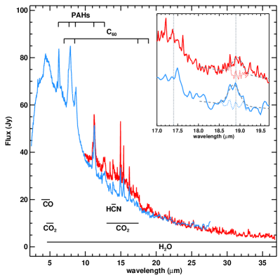
Figure 1.— The Spitzer-IRS (black, red in the online version) and speed 2 ISO-SWS (light gray, blue in the online version) observations of HR 4049 are shown. The polycyclic aromatic hydrocarbon (PAH) bands at 6.2, 7.7, 8.6, 11.2 and 12.7 $\mu$m are highlighted as well as the positions of the C₆₀ bands at 7.0, 8.5, 17.4 and 18.9 $\mu$m. The regions of the spectrum showing emission from CO, CO₂, H₂O, and HCN are also highlighted. The inset shows the 17 to 19.5 $\mu$m region of the Spitzer-IRS (black, red in the online version) and speed 1 ISO-SWS spectra (light grey, blue in the online version) highlighting the locations of the 17.4 and 18.9 $\mu$m C₆₀ bands and showing the best-fit Gaussians to the 18.9 $\mu$m bands (dashed gray lines) with the corresponding residuals for the fitting region (dotted lines).

2. Observations and Data Reduction

2.1. Spitzer-IRS

HR 4049 was observed at high spectral resolution ($R=600$) using the Infrared Spectrograph (IRS, Houck et al., 2004) aboard the Spitzer Space Telescope (Werner et al., 2004) in the short high (SH, $\lambda$ = 9.9 to 19.6 $\mu$m) mode (AOR key 4900608; program ID 93; PI D. Cruikshank) and the long high (LH, $\lambda$ = 18.7 to 37.2 $\mu$m) mode (AOR key 23711232; program ID 40896; PI J. Cami). For the LH data, we also obtained background observations (AOR key 23711488).

We used the smart data reduction package (v8.2.2, Higdon et al., 2004) as well as custom IDL routines to carry out the data reduction. Starting from the basic calibrated data (bcd), we first cleaned all data with irsclean using the campaign rogue pixel mask. When we examined the LH background observations, we found the background flux levels were fairly low (typically less than 1% of the target flux with some small unresolved spikes up to 5% of the target flux) and featureless. We thus subtracted this background from the target observations. We then combined the cleaned data collection events for each observation using a weighted average. Next, we extracted the spectra from the SH data and the background subtracted LH data using full aperture extraction in smart v8.2.2 (Higdon et al., 2004).

We then defringed the extracted spectra and trimmed the edges of the orders. Flux differences between adjacent orders were typically on the order of 5% among the SH orders and only one LH order showed a notable flux difference. We scaled adjacent orders to the median flux in the overlap region, using order 11 ($\lambda_{c}$ = 18.7 $\mu$m for SH and $\lambda_{c}$ = 35.4 $\mu$m for LH) as the reference. We then compared the spectra in overlap regions as well as the two nod positions while checking for consistency, averaged them using a weighted mean, and rebinned the resulting final spectrum.

We compared the long wavelength end of the SH spectrum and the short wavelength end of the LH spectrum and calculated a weighted mean for the overlap region. Finally, we scaled the Spitzer-IRS spectrum to the Infrared Astronomical Satellite (IRAS) flux measurement at 25 $\mu$m (scaling up by 50%). The final spectrum is presented in Fig. 1.

2.2. ISO-SWS

HR 4049 was observed twice with the Short Wavelength Spectrometer (SWS, de Graauw et al., 1996) aboard the Infrared Space Observatory (ISO, Kessler et al., 1996): on December 27th, 1995 (AOT 1, speed 1) and again on May 6th, 1996 (AOT 1, speed 2); both observations correspond to a resolving power of $\sim$300. Here, we use the speed 2 ISO-SWS data that was also presented by Cami & Yamamura (2001) and Dominik et al. (2003).

We compare the speed 2 ISO-SWS spectrum to the Spitzer-IRS observations in Fig. 1. At the longer wavelengths, the spectra agree well with one another; however, the Spitzer-IRS data exhibit a significant increase in the flux levels between 10 and 18 $\mu$m.

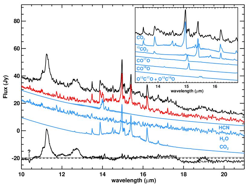
Figure 2.— The Spitzer-IRS spectrum between 10 and 20 $\mu$m (black) with the best fit model for all the molecules (dark gray or red in the online version) offset below the spectrum and models of the individual molecules below that (gray or blue in the online version) in descending order: HCN, H₂O, and CO₂. The residual without the linear component is shown at the bottom of the figure in black with the error values on the data indicated in light gray. We also fit a Gaussian to the C₆₀ feature at 19 $\mu$m in the residual and show the effect of removing this Gaussian in dashed lines. The inset shows a breakdown of the CO₂ isotopologues between 13 and 17 $\mu$m.

Table 1Temperatures, column densities, and isotope ratios for the best model fits to the data as well as the nominal 3$\sigma$ uncertainties.

	Spitzer-IRS	ISO-SWS
$\lambda_{\rm fit}$ ($\mu$m)	13.7–18	2.4–5.8; 9.5–10.5;
		14–22
Temperature (K)	500 $\pm$ 50	600 $\pm$ 50
log $N$ (CO2)	19.0 $\pm$ 0.1	17.8 $\pm$ 0.1
log $N$ (H2O)	21.6${}^{+0.1}_{-0.2}$	19.4 $\pm$ 0.1
log $N$ (HCN)	17.8 $\pm$ 0.1	…
log $N$ (CO)	…	22.0 $\pm$ 0.1
[12]C/[13]C	6${}^{+2}_{-1}$	1.6${}^{+2}_{-0.4}$
[16]O/[17]O	160${}^{+90}_{-35}$	40${}^{+23}_{-9}$
[16]O/[18]O	160${}^{+40}_{-60}$	16${}^{+4}_{-3}$
[14]N/[15]N	13${}^{+3}_{-8}$	…

3. Analysis

Fig. 1 shows the full Spitzer-IRS spectrum with emission from a variety of molecular species indicated. There are prominent features from large molecules such as polycyclic aromatic hydrocarbons (PAHs, Waters et al., 1989) and C₆₀ (Roberts et al., 2012). We have also indicated the broad emission features from CO₂ at 15 $\mu$m, the HCN feature at 14 $\mu$m and the region of the spectrum where we observe H₂O emission. There is also emission from CO and CO₂ at 4.6 and 4.2 $\mu$m respectively in the ISO-SWS spectrum.

3.1. Modeling the Spitzer Spectrum

To determine the properties of the gas in the mid-IR spectrum of HR 4049 and fully characterize the molecular emission, we created model spectra and compared them to the observational data. We used the same methods employed to build the SpectraFactory database (Cami et al., 2010b). For each model, we began with line lists detailing the frequencies and intensities of individual molecular transitions. We calculated optical depth profiles from the line lists assuming a population in local thermodynamic equilibrium (LTE) and a Gaussian intrinsic line profile with a width of 3 km s^-1. We summed the optical depth profiles for the different molecular species (including isotopologues) and then performed the proper radiative transfer calculations through an isothermal slab and smoothed the resulting model spectrum to match the SH resolution ($R=600$).

We used a 1150 K black body for the continuum and applied a non-negative least-squares (NNLS) algorithm (Lawson & Hanson, 1974) with the continuum and the molecular emission models as parameters. Then we compared our model to the observational data between 13.27 and 18 $\mu$m (to cover the CO₂ emission) and calculated $\chi^{2}_{\nu}$, the reduced $\chi^{2}$ statistic for each model to determine the quality of the fit.

We experimented with several different models to determine the best range for each of our parameters then selected the parameters for each model using an adaptive mesh algorithm. In our final fits, we varied the temperature of the molecular layer between 200 and 1000 K in increments of 100 K and column densities between 10¹⁶ and 10²² cm^-2 in increments of log$N$ = 0.2 for all molecules in this region. Additionally, we varied log(¹²C/¹³C) from 0 to 2; log(¹⁶O/¹⁸O), log(¹⁶O/¹⁷O), and log(¹⁴N/¹⁵N) from 0 to 3 in increments of 0.2.

While we began fitting only CO₂ and its isotopologues, we later included H₂O and HCN in our model spectra. In addition, we noted a small linear trend in our residuals from 13 to 17.5 $\mu$m. We do not know the origin of this trend, but we incorporated a linear component in our NNLS routine to compensate for this residual.

4. Results

We present the parameters for our best fit model in Table 1 and the 10 to 20 $\mu$m region of the Spitzer-IRS spectrum with our best fit model in Fig. 2. We focus on the H₂O emission at LH wavelengths in Fig. 3 and we compare the models to the full spectrum Spitzer-IRS and our predictions at ISO-SWS wavelengths in Fig. 4. We find a $\chi^{2}_{\nu}$ of 3.5 for the fit to the Spitzer-IRS observation and a good representation of the molecular emission features within our fitting region.

When we compare the predictions from our model at longer and shorter wavelengths to the spectrum, we find that the spectral features are also fit remarkably well. The majority of the molecular features in the LH spectrum, for example, appear to be from H₂O emission. In addition, the spikes on the PAH features at 11.2 and 12.7 $\mu$m disappear and some of the smaller PAH features become evident.

4.1. CO₂

The Spitzer-IRS spectrum shows prominent emission from the CO₂ isotopologues observed by Cami & Yamamura (2001) in addition to others (e.g. the O[13]C[17]O and O[13]C[18]O peaks which Cami & Yamamura (2001) were unable to separate due to the lower spectral resolution of ISO-SWS). To model the emission from CO₂, we used line lists from the 1000 K Carbon Dioxide Spectroscopic Database (CDSD, Tashkun et al., 2003) including the ¹³CO₂, CO¹⁷O, CO¹⁸O, O¹³C¹⁷O, and O¹³C¹⁸O isotopologues.

Though our single layer LTE model reproduces the majority of the CO₂ features very well, (see Fig. 2), we find that the best fit model tends to slightly overestimate the flux relative to the local continuum between 14.2 and 14.7 $\mu$m while underestimating the flux between 16.7 and 17.6 $\mu$m (which may be due to some contribution from C₆₀ at the long wavelength end). We also find high optical depths across most of our fit region with this model.

There are also small spikes which may be due to a slight temperature stratification in the CO₂ layer. For example, we note a small feature in the residual spectrum at 16.64 $\mu$m which could be due to the transition between the $4\nu_{2}^{4}$ and $3\nu_{2}^{1}$ levels, which suggests the presence of additional hotter gas. We also observe a small residual peak at 14.98 $\mu$m near the main CO₂ band, which is a combination of the $\nu_{2}$ bending mode at 14.98 $\mu$m ($1\nu_{2}^{1}$ to the ground state) and subsequent hot bands which are each shifted slightly to the blue; the presence of residual emission at 14.98 $\mu$m thus suggests the presence of some colder CO₂. The high optical depths of the gas could make the appearance of the bands more sensitive to these types of temperature variations; however, these residuals are relatively small, suggesting that most of the emission originates from a relatively thermally homogeneous layer.

We also note some small residual emission at 15.04 and 15.10 $\mu$m, which could be due to additional emission from the main $\nu_{2}$ bands of the OC[17]O and OC[18]O isotopologues respectively.

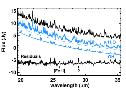
Figure 3.— The Spitzer-IRS spectrum of HR 4049 (black) with the best fit model for H₂O and a model for OH at the same temperature and column density offset below the spectrum (gray or blue in the online version). The dotted gray (blue in the online version) lines indicate the black body continuum under the H₂O and OH models.

4.2. H₂O and OH

After including all CO₂ isotopologues in our models, many weaker emission features remained in the residuals of this region. We noticed that several features are consistent with emission from water vapor. Thus, we recalculated our models including optical depth profiles for H₂O using line lists from Partridge & Schwenke (1997, including the H${}_{2}^{17}$O and H${}_{2}^{18}$O isotopologues).

We find an extremely high column density for H₂O and a much better correspondence to the results than for CO₂, not only in the region we chose to fit, but also at longer and shorter wavelengths in the Spitzer-IRS spectrum. Upon careful examination of the residuals in Fig. 2, one may note that the spikes atop the 11.2 and 12.7 $\mu$m PAH features disappear almost completely and remarkably, the 12 $\mu$m PAH feature becomes apparent though it was previously hidden by H₂O emission. Furthermore, the 18.9 $\mu$m C₆₀ feature becomes much more prominent and clear when H₂O emission is removed. In Figs. 3 and 4, it is also clear that H₂O accounts for the bulk of the features in the LH spectrum since the residuals contain relatively few remaining spectral features. This observation also confirms the earlier detection of water in HR 4049 in the near-IR by Hinkle et al. (2007).

Since OH was also detected by Hinkle et al. (2007) at $\sim$3 $\mu$m, and since it has many features in this wavelength range, we included it in our models between 13.24 and 18 $\mu$m. However, we were unable to detect OH in this region of the spectrum. We were also unable to fit any OH using only H₂O and OH between 20 and 35 $\mu$m. In Fig. 3, we show a comparison between model spectra of H₂O and OH using the same temperatures and column densities at LH wavelengths. We note that while there appear to be many features in our residuals which are consistent with emission from OH, it is not possible to reliably fit the OH features due to extensive contamination from H₂O.

4.3. HCN

When all the CO₂ and H₂O isotopologues are included in our models, there is still significant residual emission at 14.04 $\mu$m, where the CH bending mode of HCN is often seen in evolved stars. Indeed, the SpectraFactory catalogue (Cami et al., 2010b) reveals a clear HCN molecular band at this wavelength, thus we include it in our model calculations using line lists from the HITRAN 2008 database (Rothman et al., 2009, including the H¹³CN and HC¹⁵N isotopologues).

We determine a column density for HCN which is much lower than that of CO₂ and H₂O (log$N=17.8$), which suggests that it is less abundant. We included isotopologues of HCN containing [13]C and [15]N which appear slightly to the red of the main isotopologue and are thus able to find [14]N/[15]N of 13${}^{+3}_{-5}$. With only one band containing this isotope though, we do not consider our ratio here to be especially reliable.

4.4. Fullerenes

Since its detection in the young planetary nebula Tc 1 by Cami et al. (2010a), C₆₀ has been reported in other evolved binary systems (Gielen et al., 2011b) and it was recently reported in HR 4049 by Roberts et al. (2012), who detected the 17.4 and 18.9 $\mu$m features.

Indeed, the 18.9 $\mu$m feature is clear (and also present in the ISO-SWS speed 1 observations, see the inset of Fig. 1) and when we subtract our best fit H₂O model, the feature becomes much more prominent (see Fig. 2). Fitting the 18.9 $\mu$m C₆₀ feature in the residual spectrum with a Gaussian, we determine a FWHM of 0.40 $\mu$m and a central wavelength of 18.98 $\mu$m. This is a much narrower band than found by Roberts et al. (2012), who reported a FWHM of 0.64 $\mu$m. This difference may be due to the presence of the water features, which makes the band appear broader.

The 17.4 $\mu$m feature is buried in the optically thick CO₂ emission, so we cannot measure it accurately. Additionally, since no observations were taken by the IRS short low (SL; $R=90$ to $127$, $\lambda=5.2$ to $14.5$ $\mu$m) mode, the 7 and 8.5 $\mu$m features for C₆₀ would only appear in the ISO-SWS spectrum. However, we do not see them, which could be due to a combination of the sensitivity of ISO-SWS and the often weak nature of these features.

4.5. PAHs

The spectral region covered by the Spitzer-IRS observations covers only the 11.2 and 12.7 $\mu$m PAH features. These bands also appear in the ISO-SWS spectrum alongside features at 6.2, 7.7 and 8.6 $\mu$m. The PAH features in the ISO-SWS spectrum of HR 4049 were described in detail by Beintema et al. (1996) and Molster et al. (1996) and are class B (Peeters et al., 2002).

Examining the residual spectra (see Fig. 2 especially), we note that some of the less prominent PAH features become clear when the H₂O emission is removed from the spectrum. For instance, the 12 $\mu$m feature from CH out-of-plane duo-modes and the weak, broad feature at 10.7 $\mu$m from PAH cations (Hony et al., 2001) are not clear in the original spectrum, but stand out in the residual. In addition, we find that the profiles of the already prominent PAH features become clearer when the H₂O emission is removed.

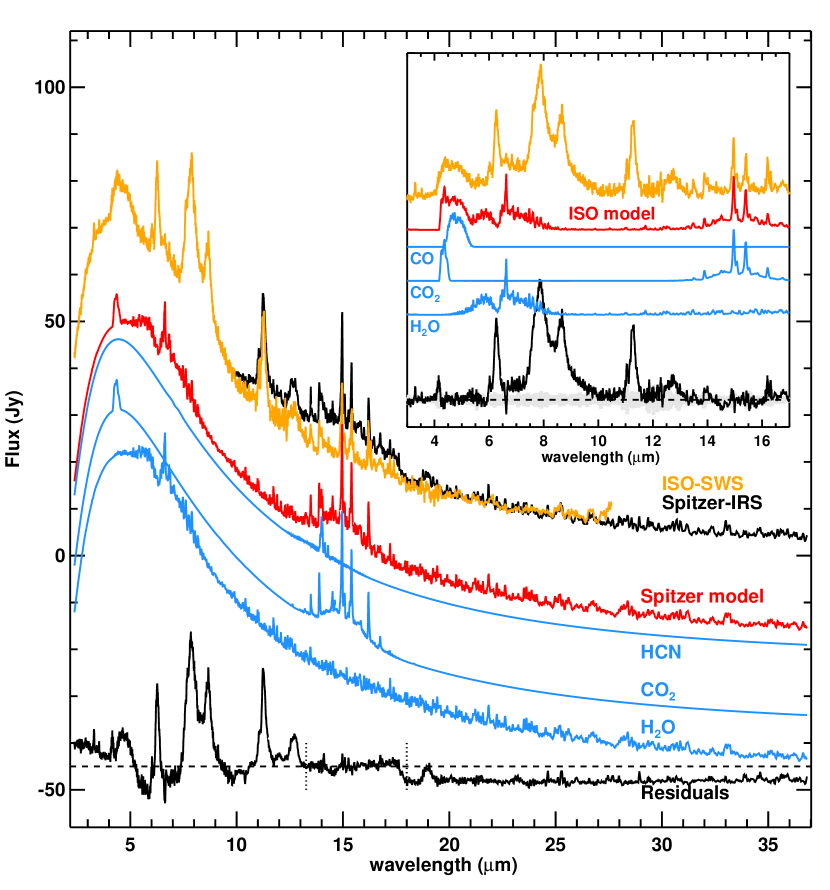
Figure 4.— Main plot: Spitzer-IRS spectrum (black) and ISO-SWS spectrum (light grey or orange in the online version) for HR 4049 with the best fit model (dark gray or red in the online version) to the Spitzer-IRS spectrum and models for the individual components for CO₂, H₂O, and HCN offset below the spectrum (gray or blue in the online version) as well as the residuals (black). The vertical dotted lines indicate the region of the spectrum used to fit the model to the Spitzer-IRS data. The model outside of these wavelength ranges (including the ISO-SWS spectrum) is the prediction based on these best fit parameters. Inset: Model fit to the ISO-SWS spectrum, with the best fit model (dark gray or red in the online version) and individual components for CO, CO₂ and H₂O offset below the spectrum (gray or blue in the online version). The residuals for this model are shown in black and the uncertainties in the data are shown in light gray.

4.6. Residual Features

There are a few interesting features in the residual spectrum. For instance, we note a small absorption feature at 10.38 $\mu$m. This feature was previously observed in the carbon-rich pre-planetary nebula SMP LMC 11 (catalog ) by Malek et al. (2012), who suggested that this feature is molecular in nature, but they were unable to identify the carrier.

As described above, a few of the residual features in the LH spectrum may be due to OH emission. However, we also observe an emission feature at 25.99 $\mu$m which could be due to a fine-structure line from [Fe II] (see Fig. 3). To confirm that this feature is real, we examined the background observations and determined that this region of the spectrum was featureless. Then we examined both nod positions in the background-subtracted spectrum and noted that it appeared in both.

This transition is from the J=7/2 to J=9/2 (ground) level in the a⁶D state. The next transition would appear at 35.35 $\mu$m (J=5/2 to J=7/2), but we do not observe a clear feature from this line. Instead, we observe a large and broad spike which appears to be from noise (S/N decreases toward the end of the LH spectrum). If we assume that the [Fe II] is at the same temperature as the molecular layer (500 K), we can estimate the strength of the expected emission at 35.35 $\mu$m. Using the method described in Justtanont et al. (1999), we find that the 35.35 $\mu$m line should be 80% as strong as the 25.99 $\mu$m line, which could be hidden by this spike in the noise.

Plateau Emission

In addition to the small emission features in our residuals, we note that we are unable to properly reproduce the continuum beyond $\sim$17.6 $\mu$m. Indeed, examining Figs. 2 and 4, we see that we systematically overestimate the continuum emission at LH wavelengths. As well, we note that one of the major differences between the Spitzer-IRS and ISO-SWS spectra in Fig. 1 is the presence of emission from a continuum-like “plateau” under the CO₂ emission in the Spitzer spectrum.

If we force the dust continuum to represent the LH continuum more accurately, we find that our models cease to reproduce the narrow emission bands from CO₂. If we instead fit the narrow emission features, we overestimate the dust continuum at LH wavelengths. We have chosen to use a model which reproduces the narrow CO₂ features, but we note that the dust continuum from our best fit model is much higher than it should be as a result.

Part of this plateau emission is likely due to the presence of C₆₀. However, since the residual flux is much wider than the 17.4 $\mu$m C₆₀ feature, this will not account for all of this plateau. In addition, the carrier of this plateau emission appears to have formed between the observations by ISO and Spitzer since this is perhaps the most obvious difference between the two spectra. We therefore considered two possible sources for this plateau emission.

First, we considered the possibility that this could be due to broad PAH emission from C-C-C bending modes, which has been observed to form a continuum between 15 and 20 $\mu$m (e.g.  Van Kerckhoven et al., 2000; Boersma et al., 2010). These PAH plateaus also often show narrow features at 16.4, 17.4 and 18.9 $\mu$m along with a weak 15.8 $\mu$m feature (Tielens et al., 1999; Moutou et al., 2000). However, we do not see any obvious PAH features to the red of the 12.7 $\mu$m feature. Therefore, we consider it unlikely that this plateau is due to PAH emission.

Another possible candidate for this plateau emission is CO₂. While our CO₂ models predict some continuum-like emission, it is not enough to match the plateau we observe. We do find high optical depths for CO₂ ($\tau_{\rm max}\approx 160$ for the main isotopologue using a line width of 3 km s^-1, this would decrease to $\tau_{\rm max}\approx 52$ for 10 km s^-1) as well as some evidence for temperature stratification in the residuals and possibly recent CO₂ formation which could result in some non-LTE emission. We therefore consider that the plateau emission could be due to CO₂ emission that our models are unable to fit properly. We will explore this possibility further in Section 5.4. We note that a similar plateau was also observed in IRAS 06338 (catalog ) (Gielen et al., 2011b) and was attributed to optically thick CO₂ emission.

4.7. ISO Spectrum

CO₂, H₂O and HCN potentially all have features at the shorter wavelengths covered by ISO-SWS in addition to the features we observe in the Spitzer-IRS spectrum. We thus decided to compare the predictions from our model at these wavelengths to the ISO-SWS spectrum. We extended our model spectra to shorter wavelengths and smoothed the spectrum covered only by the ISO-SWS spectrum to a resolution of 300 to match these data. We present our prediction for these bands in the main plot of Fig. 4.

These predictions do not appear to fit the ISO-SWS spectrum on first sight. However, some of the features do appear to be reproduced. Examining the CO₂ feature at 4.2 $\mu$m, we note that this band is heavily blended with the much broader CO emission band at 4.6 $\mu$m. It appears, however, that the CO₂ feature within this broader band is reproduced reasonably well.

If we examine our predictions for the H₂O spectrum, there is a broad emission feature between 5 and 8 $\mu$m. It is difficult to assess how well this broad band reproduces the spectrum in these regions due to the presence of the CO emission feature and the PAH features. However, our model predicts a fairly strong H₂O feature at 6.62 $\mu$m which is much weaker in the ISO-SWS spectrum.

Finally, although HCN also has an overtone mode at $\sim$7 $\mu$m, our models do not predict it at these temperatures and column densities.

Since the ISO-SWS spectrum has a much larger wavelength coverage, it covers additional molecular bands (such as the 4.2 $\mu$m CO₂ feature) and species (CO at 4.6 $\mu$m), so we decided to fit this spectrum as well. We used the same techniques described for fitting the Spitzer-IRS spectrum, but we included CO in our model (using line lists from Goorvitch, 1994, including the ¹³CO, C¹⁷O and C¹⁸O isotopologues) and excluded HCN. We fit the spectrum in several regions to include as many molecular features as possible while excluding features we cannot fit (e.g. the PAHs). Thus, we used three fitting regions, first, between 2.4 and 5.8 $\mu$m, then from 9.5 to 10.5 $\mu$m and finally from 14 to 22 $\mu$m.

The parameters for our best fit are presented in Table 1 and this model is compared to the 3 to 17 $\mu$m region of the ISO-SWS spectrum in the inset of Fig. 4. In our direct fit to the ISO-SWS spectrum, we find that the fit in the 4 $\mu$m region is greatly improved with the addition of CO and a more appropriate scaling factor for the continuum. However, we note that there are still issues in the H₂O emission at 6.62 $\mu$m where we fit a large emission spike which does not appear in the spectrum. In addition, there are some residuals at $\sim$16 $\mu$m.

Time dependence

When we compare the ISO-SWS and Spitzer observations, we find that there is a dramatic increase in emission between 10 and 18 $\mu$m. If we subtract a 1150 K black body continuum from each spectrum and integrate the remaining flux between 13.4 and 16.8 $\mu$m, we find that the flux from molecular emission has more than doubled in this region between the time of the ISO and Spitzer observations (from $\sim 2\times 10^{-10}$ W m² to $\sim 5\times 10^{-10}$ W m²).

5. Discussion

The better quality of the Spitzer-IRS data and current line lists allow a much more in-depth analysis of the gas than was previously possible. As we shall see, many of the results of this analysis have important consequences for the properties of the circumbinary disk.

5.1. Isotopic Ratios

We remind the reader that in the optically thin limit, Cami & Yamamura (2001) determined that HR 4049 was extremely enriched in [17]O and [18]O ([16]O/[17]O = $8.3\pm 2.3$; [16]O/[18]O = $6.9\pm 0.9$). In a subsequent study of the near-IR CO bands, Hinkle et al. (2007) found isotopic ratios consistent with solar values and they suggested that the ratios determined by Cami & Yamamura (2001) were incorrect because the CO₂ emission in HR 4049 is actually optically thick. Based on our models, we are able to confirm the suggestion by Hinkle et al. (2007) that the CO₂ is optically thick, but we determine a ratio of 160${}^{+90}_{-35}$ for [16]O/[17]O and 160${}^{+40}_{-60}$ for [16]O/[18]O, indicating some enrichment in [17]O and [18]O relative to solar values ([16]O/[17]O = 2700, [16]O/[18]O = 479, Anders & Grevesse (1989); Scott et al. (2006)). In addition, these isotopes are enriched relative to tyical AGB stars (where both are on the order of a 10² to 10³, see Harris & Lambert, 1984; Harris et al., 1985b, 1987, 1988; Smith & Lambert, 1990). Indeed, the enrichment of [17]O and [18]O in HR 4049 appears to be similar to that of the Ba star HD 101013 (¹⁶O/¹⁷O = 100${}^{+100}_{-50}$, ¹⁶O/¹⁸O = 60${}^{+100}_{-30}$, Harris et al., 1985a).

There are also recent detections of OC¹⁸O in two other binary post-AGB objects: EP Lyr (catalog ) and HD 52961 (catalog ) which both show enrichment in [18]O (¹⁶O/¹⁸O of 19 for EP Lyr and 100 for HD 52961, Gielen et al., 2009). As well as a study of [18]O enrichment in R Coronae Borealis stars in which [16]O/[18]O ratios less than one were found (Clayton et al., 2007).

We also note that the values we find here for the enrichment of [17]O and [18]O are more suitable to the scenario proposed by Lugaro et al. (2005) who suggested that the isotopic ratios for oxygen in HR 4049 could be due to nova nucleosynthesis; though HR 4049 lacks the UV flux for a typical white dwarf companion (Monier & Parthasarathy, 1999). However, due to the high optical depths we find, our values are poorly determined and our uncertainties on these values are likely to be larger than we find from our models. We also suggest that there may be similar issues with the [16]O/[18]O values in the other post-AGB objects for the same reason.

Our best fit models appear to indicate an enrichment in [13]C, with [12]C/[13]C of 6${}^{+2}_{-1}$. This relatively low value agrees with an early termination of the AGB due to accelerated mass loss along the orbital plane of the binary (Iben & Livio, 1993). This has been observed in other binary post-AGB objects such as EP Lyr (Gielen et al., 2008). However, optically thick CO₂ emission also makes this ratio uncertain.

5.2. Gas Distribution and Disk Structure

From our models, we find that not only is the CO₂ emission optically thick, but the gas is optically thick across the entire spectrum (e.g. $\tau>10$ for H₂O across the entire Spitzer-IRS spectrum). This has some very important ramifications. For instance, when the gas is optically thick, the flux will scale with the emitting area, thus we are able to estimate the spatial extent of the gas using our models.

When we calculate our models, we obtain a scale factor ($f$) which relates $I_{\nu}$ from our radiative transfer calculations to $F_{\nu}$. We are able to relate this scale factor to the surface area ($A$) of the emitting layer such that $f=A/4D^{2}$, where $D$ is the distance to HR 4049.

From our model fit to the Spitzer-IRS data, we find a value of $1.60\times 10^{9}$ for $f$. If we use a distance of 640 pc for HR 4049 (as described by Acke et al., 2013), this scale factor corresponds to a projected area of 1117 AU². If we perform the same analysis using our best fit to the ISO-SWS spectrum (with $f=1.57\times 10^{9}$), we find a projected area of 1097 AU², which agrees reasonably well with the emitting region we estimate from our Spitzer-IRS data. Since the scale factors we determine have not changed much between the ISO and Spitzer observations despite the differences in column densities between the two models, this also supports our claim of optically thick gas.

If we then assume an inclination angle of 60^∘ (which is agreed upon by both current models for the disk), we find an actual emitting surface of 1290 AU² for our molecular emission. If we consider how this surface area would fit into the current disk models, we note that this would not fit on the inner rim of the wall model.

This suggests that the gas belongs to a radially extended disk instead. If we assume that the gas exists some distance from the center of the binary system, we can estimate the maximum extent of the disk. Were the gas to originate 10 AU from the binary (as the dust in the wall model, Dominik et al., 2003), it would extend to a distance of 23 AU. If the gas begins at 15 AU from the binary (based on the interferometric observations by Acke et al., 2013), it would extend to 25 AU, a distance which agrees well with the maximum radial extent of the disk determined from the interferometric observations by Acke et al. (2013).

It would be reasonable to suppose that the gas is mixed in with any dust in the circumbinary disk of HR 4049. As described by Dominik et al. (2003), dust grains in a gas-rich disk tend to settle toward the midplane of the disk, so the gas we observe could form a sort of atmosphere on the outside of the disk. There could also be more gas inside the disk which we are unable to observe since this atmosphere is optically thick. However, the gas on the inside of the disk could contribute to the opacity of the disk by providing some continuum-like emission similar to that we observe in our models.

As the LTE models reproduce the emission spectrum well and the gas appears to be reasonably warm (500 K), we find that we cannot reconcile our observations to a wall-type model for the dust. The wall model contains cold dust beyond the inner rim of the disk (Dominik et al., 2003), which would result in cold gas in this region. Instead, we observe a large region of warm gas so we find this sort of model improbable.

It would also be difficult to reconcile our observations to the disk model presented by Acke et al. (2013) in which the dust is optically thin. Acke et al. (2013) include gas in their disk to determine the scale height, however CO₂ and H₂O are both excellent at trapping infrared radiation, especially at high column densities like those we observe in this disk and these effects are not included in their model.

Since these molecules are largely transparent at optical wavelengths, the stellar radiation will warm the dust grains. These grains will then re-emit this radiation in the infrared which will be absorbed and re-emitted by the gas in the disk, effectively trapping the radiation inside the disk. This will not only have the effect of warming the disk overall, but it will also keep the temperature relatively homogenous throughout the disk. Thus the disk could have the sort of narrow temperature range suggested by Dominik et al. (2003), who determined that the SED of HR 4049 can be fit either by a 1150 K black body or by the sum of several equally weighted black bodies within a range of 880 K $\leq T\leq$ 1325 K.

However, in LTE, a gas cannot appear in emission in front of a hotter background source. Thus, we will explore alternate excitation mechanisms which could result in bands which emit in a way which appears similar to LTE in Section 5.4.

5.3. Total Gas Mass

Using the projected size for the emitting region and our column densities, we can estimate lower limits for the masses of the molecular species we observe in this system. Then, combining these with photospheric abundances, we can estimate a lower limit for the total mass of the gas in the circumbinary environment of HR 4049.

From our model fit to the Spitzer-IRS data, we calculate a mass of $9.19\times 10^{-8}$ M_☉ for CO₂, $1.50\times 10^{-5}$ M_☉ for H₂O and $3.56\times 10^{-9}$ M_☉ for HCN. Similarly, for the ISO-SWS model, we find masses of $5.69\times 10^{-9}$ M_☉ for CO₂, $9.28\times 10^{-8}$ M_☉ for H₂O and $5.74\times 10^{-5}$ M_☉ of CO.

Since the gas is oxygen-rich, we use the carbon abundance determined by Waelkens et al. (1991b, log $N_{C}/N_{H}=8.41-12$) along with the number of carbon-containing molecules and determine a lower limit for the total gas mass of $7.98\times 10^{-3}$ M_☉ in the disk. This estimate is higher than the mass estimated by Dominik et al. (2003), who estimated $2.85\times 10^{-4}$ M_☉ for the total mass of the disk. This could indicate a higher gas to dust ratio in the disk (they use a value of 100) or the presence of even more dust in this system than predicted by the wall model. If we compare our estimate for the gas mass to the dust mass from Acke et al. (2013, in which $M_{\rm dust}=(1.0\pm 0.4)\times 10^{-8}$ M_☉), we find a gas-to-dust ratio of approximately 10⁶. This appears unreasonably high, however this is the estimated mass for only the small grains in the disk, which are responsible for the near- and mid-IR SED as well as the optical and UV extinction. Their model also includes a cold dust component to reproduce the flux at the far-IR and submm wavelengths, which would contain more mass.

Since the gas is optically thick, this estimate will not include all the gas in the system (e.g. any gas beyond the optically thick layer or on the side of the disk inclined away from us is not included). In addition, since the majority of the gas included in our estimate is CO which only appears in the ISO-SWS spectrum, this may not describe the current gas mass since, as we will describe presently, it appears there is significant ongoing gas formation in HR 4049.

5.4. Time Evolution

It is somewhat surprising to see that the CO₂ flux has increased by a factor of 2.5 between the ISO-SWS and Spitzer-IRS observations (see Section 4.7). Since we scaled the Spitzer-IRS observations to match the IRAS flux point at 25 $\mu$m, we considered that this could be an issue in our comparison of these observations. However, the ISO-SWS spectrum was also scaled to the same point so this is unlikely to change our observation. Furthermore, it is not just the flux that has changed under the CO₂ emission features, but also the shape of the “continuum” and features in this region. Thus, it appears that the change in the emission features is real.

We compared the phase between the two observations using the phase information from Bakker et al. (1998). The SH observations were taken at a phase ($\phi$) of 0.844, while the ISO-SWS speed 2 observations were taken at $\phi=0.041$, near the photometric minumum. There are also the ISO-SWS speed 1 observations available, which were taken at a similar phase as the Spitzer-IRS observations ($\phi=0.738$).

We thus compared the two ISO-SWS observations to see if there was a change in this region of the spectrum which could be attributed to phase. When we did so, we found that the spectra of the speed 1 and speed 2 ISO-SWS observations were roughly the same within the uncertainty mesurements on the fluxes.

Thus, we conclude that the amount of emitting CO₂ gas we can observe has increased between the observations by ISO-SWS and those by Spitzer-IRS observations. If the gas were optically thin, this would imply that CO₂ has been forming at a rate of $3.68\times 10^{-9}$ M_☉ yr^-1 assuming a constant formation rate. We note that this represents a considerable and rapid increase in CO₂ in the system, however, as we discovered, the CO₂ emission in the mid-IR spectrum is not optically thin so this represents a lower limit to the increase in CO₂. In addition, we cannot know whether the formation has been continuous between the observations so this is a crude estimate for the formation rate.

While Bakker et al. (1996) reported a mass-loss rate from HR 4049 of $(6\pm 4)\times 10^{-7}$ M_☉ yr^-1, the amount of carbon and oxygen in the stellar winds is insufficient to permit the formation of so much new material. Therefore, we consider that the CO₂ we observe is forming from the interaction between the stellar wind and the dust disk.

The ongoing formation of oxygen-rich gas thus suggests that the dust contains an oxygen-rich component (e.g. silicates) and the absence of features from these dust species in the spectrum would therefore be due to obscuration of these features by optically thick gas; or by the dust being optically thick or perhaps　being composed of large dust grains which have a smooth opacity. If the dust is primarily oxygen-rich, then HR 4049 would also be consistent with other post-AGB binaries in this regard　(e.g.  Gielen et al., 2011a).

While this may appear to be inconsistent with the fact that small dust grains are required to explain the optical and UV extinction, it was noted by Dominik et al. (2003) that the extinction at short wavelengths and the IR excess do not need to be caused by the same population of dust grains. Thus, although the optical and UV extinction is described well by a population of small grains of amorphous carbon or metallic iron as described by Acke et al. (2013), these grains cannot be the only dust component in the disk since they cannot allow the formation of the oxygen-rich gas we observe here.

The presence of small carbonaceous grains in the upper region of the disk could thus contribute to the extinction at short wavelengths while a population of oxygen-rich grains could contribute to part of the IR emission.

The evidence for ongoing formation of gas in the circumbinary disk of HR 4049 also suggests that the molecules are not actually in LTE, and the emission we observe may be due to pumping—either radiative pumping or formation pumping. In both cases, pumping results in a large fraction of molecules in highly excited vibrational states, either through absorption of higher energy photons (near-IR or even UV) or alternatively as a direct result of the formation of the molecules which leaves them in the excited states. After being pumped, they cascade down by emission of the IR photons we observe. Pumping would thus always produce emission at mid-IR wavelengths even when in front of hot dust. Superficially, such emission spectra could resemble LTE models; their main difference would be the presence of many bands from higher vibrational levels. This could help explain the plateau emission as a forest of CO₂ emission lines from higher energies.

It is thus possible that the CO₂ and H₂O are being radiatively pumped the hot dust, but this has not been directly observed. Note that all these species have strong electronic absorption bands at UV wavelengths which could be the source of the pumping through absorption of stellar radiation as well. Given the high column densities of these species, it would be interesting to investigate whether this could be a contributing source of the observed UV deficit in HR 4049 (Lamers et al., 1986). Formation pumping is certainly an appealing alternative, but is not well studied. While models exist for the formation pumping of H₂ after formation on dust grain surfaces (e.g.  Gough et al., 1996; Takahashi & Uehara, 2001), but to our knowledge no such models exist for CO₂ or H₂O.

Finally, we note that while it appears that gas has been forming in the disk of HR 4049, the overall emitting surface does not seem to have changed significantly (remaining at $\sim$1300 AU²). This agrees very well with the idea that the disk is relatively stable and long-lived (also supported by the unchanging CO overtone absorption observed between the observations of Lambert et al. (1988) and those by Hinkle et al. (2007)).

Dominik et al. (2003) described how a gas-rich disk (such as the one we describe) would tend to settle toward the midplane and expand outward. Using a gas-to-dust ratio of 100 and an initial scale height of 4 AU, they estimated that the scale height of the disk would decrease by half in 150 years. This effect could be mitigated by a higher gas-to-dust ratio and we suggest that the gas-to-dust ratio is likely to be greater than 100 in this environment. Indeed, if the dust is being slowly destroyed by stellar wind and gas is being formed, this ratio is likely to be increasing.

6. Conclusion

The Spitzer-IRS observations clearly reveal that the molecular gas in the circumbinary disk of HR 4049 is optically thick at infrared wavelengths and that the emission originates from a radially extended disk. The gas causes a strong greenhouse effect that plays a significant role in determining the thermal structure in the disk. Including the effect of optical depth, we determine that there is less of an enrichment in ¹⁷O and ¹⁸O than previously reported. Additionally, changes in the observed flux between ISO and Spitzer observations suggest ongoing chemical processing of oxygen-rich dust.

References

- Acke et al. (2013) Acke B., Degroote P., Lombaert R., et al., 2013, A&A 551, A76
- Anders & Grevesse (1989) Anders E., Grevesse N., 1989, Geochim. Cosmochim. Acta 53, 197
- Bakker et al. (1998) Bakker E.J., Lambert D.L., Van Winckel H., et al., 1998, A&A 336, 263
- Bakker et al. (1996) Bakker E.J., van der Wolf F.L.A., Lamers H.J.G.L.M., et al., 1996, A&A 306, 924
- Beintema et al. (1996) Beintema D.A., van den Ancker M.E., Molster F.J., et al., 1996, A&A 315, L369
- Boersma et al. (2010) Boersma C., Bauschlicher C.W., Allamandola L.J., et al., 2010, A&A 511, A32
- Cami et al. (2010a) Cami J., Bernard-Salas J., Peeters E., Malek S.E., 2010a, Science 329, 1180
- Cami et al. (2010b) Cami J., van Malderen R., Markwick A.J., 2010b, ApJS 187, 409
- Cami & Yamamura (2001) Cami J., Yamamura I., 2001, A&A 367, L1
- Clayton et al. (2007) Clayton G.C., Geballe T.R., Herwig F., Fryer C., Asplund M., 2007, ApJ 662, 1220
- de Graauw et al. (1996) de Graauw T., Haser L.N., Beintema D.A., et al., 1996, A&A 315, L49
- Dominik et al. (2003) Dominik C., Dullemond C.P., Cami J., van Winckel H., 2003, A&A 397, 595
- Geballe et al. (1989) Geballe T.R., Noll K.S., Whittet D.C.B., Waters L.B.F.M., 1989, ApJ 340, L29
- Gielen et al. (2011a) Gielen C., Bouwman J., van Winckel H., et al., 2011a, A&A 533, A99
- Gielen et al. (2011b) Gielen C., Cami J., Bouwman J., Peeters E., Min M., 2011b, A&A 536, A54
- Gielen et al. (2009) Gielen C., van Winckel H., Matsuura M., et al., 2009, A&A 503, 843
- Gielen et al. (2008) Gielen C., van Winckel H., Min M., Waters L.B.F.M., Lloyd Evans T., 2008, A&A 490, 725
- Goorvitch (1994) Goorvitch D., 1994, ApJS 95, 535
- Gough et al. (1996) Gough S., Schermann C., Pichou F., et al., 1996, A&A 305, 687
- Guillois et al. (1999) Guillois O., Ledoux G., Reynaud C., 1999, ApJ 521, L133
- Harris & Lambert (1984) Harris M.J., Lambert D.L., 1984, ApJ 285, 674
- Harris et al. (1987) Harris M.J., Lambert D.L., Hinkle K.H., Gustafsson B., Eriksson K., 1987, ApJ 316, 294
- Harris et al. (1985a) Harris M.J., Lambert D.L., Smith V.V., 1985a, ApJ 292, 620
- Harris et al. (1985b) Harris M.J., Lambert D.L., Smith V.V., 1985b, ApJ 299, 375
- Harris et al. (1988) Harris M.J., Lambert D.L., Smith V.V., 1988, ApJ 325, 768
- Higdon et al. (2004) Higdon S.J.U., Devost D., Higdon J.L., et al., 2004, PASP 116, 975
- Hinkle et al. (2007) Hinkle K.H., Brittain S.D., Lambert D.L., 2007, ApJ 664, 501
- Hony et al. (2001) Hony S., Van Kerckhoven C., Peeters E., et al., 2001, A&A 370, 1030
- Houck et al. (2004) Houck J.R., Roellig T.L., van Cleve J., et al., 2004, ApJS 154, 18
- Iben & Livio (1993) Iben, Jr. I., Livio M., 1993, PASP 105, 1373
- Justtanont et al. (1999) Justtanont K., Tielens A.G.G.M., de Jong T., et al., 1999, A&A 345, 605
- Kessler et al. (1996) Kessler M.F., Steinz J.A., Anderegg M.E., et al., 1996, A&A 315, L27
- Lambert et al. (1988) Lambert D.L., Hinkle K.H., Luck R.E., 1988, ApJ 333, 917
- Lamers et al. (1986) Lamers H.J.G.L.M., Waters L.B.F.M., Garmany C.D., Perez M.R., Waelkens C., 1986, A&A 154, L20
- Lawson & Hanson (1974) Lawson C.L., Hanson R.J., 1974, Solving least squares problems
- Lugaro et al. (2005) Lugaro M., Pols O., Karakas A.I., Tout C.A., 2005, Nuclear Physics A 758, 725
- Malek et al. (2012) Malek S.E., Cami J., Bernard-Salas J., 2012, ApJ 744, 16
- Mathis & Lamers (1992) Mathis J.S., Lamers H.J.G.L.M., 1992, A&A 259, L39
- Molster et al. (1996) Molster F.J., van den Ancker M.E., Tielens A.G.G.M., et al., 1996, A&A 315, L373
- Monier & Parthasarathy (1999) Monier R., Parthasarathy M., 1999, A&A 341, 117
- Moutou et al. (2000) Moutou C., Verstraete L., Léger A., Sellgren K., Schmidt W., 2000, A&A 354, L17
- Partridge & Schwenke (1997) Partridge H., Schwenke D., 1997, ”Journal of Chemical Physics” 106, 4618
- Peeters et al. (2002) Peeters E., Hony S., Van Kerckhoven C., et al., 2002, A&A 390, 1089
- Roberts et al. (2012) Roberts K.R.G., Smith K.T., Sarre P.J., 2012, MNRAS 421, 3277
- Rothman et al. (2009) Rothman L.S., Gordon I.E., Barbe A., et al., 2009, J. Quant. Spec. Radiat. Transf. 110, 533
- Scott et al. (2006) Scott P.C., Asplund M., Grevesse N., Sauval A.J., 2006, A&A 456, 675
- Smith & Lambert (1990) Smith V.V., Lambert D.L., 1990, ApJS 72, 387
- Takada-Hidai (1990) Takada-Hidai M., 1990, PASP 102, 139
- Takahashi & Uehara (2001) Takahashi J., Uehara H., 2001, ApJ 561, 843
- Tashkun et al. (2003) Tashkun S.A., Perevalov V., Teffo J.L., D. L.N., 2003, Journal of Quantitative Spectroscopy and Radiative Transfer 82, 165
- Tielens (2008) Tielens A.G.G.M., 2008, ARA&A 46, 289
- Tielens et al. (1999) Tielens A.G.G.M., Hony S., van Kerckhoven C., Peeters E., 1999, In: Cox P., Kessler M. (eds.), The Universe as Seen by ISO, vol. 427 of ESA Special Publication, p. 579
- Van Kerckhoven et al. (2000) Van Kerckhoven C., Hony S., Peeters E., et al., 2000, A&A 357, 1013
- Van Winckel et al. (1995) Van Winckel H., Waelkens C., Waters L.B.F.M., 1995, A&A 293, L25
- Waelkens et al. (1991a) Waelkens C., Lamers H.J.G.L.M., Waters L.B.F.M., et al., 1991a, A&A 242, 433
- Waelkens et al. (1991b) Waelkens C., Van Winckel H., Bogaert E., Trams N.R., 1991b, A&A 251, 495
- Waters et al. (1989) Waters L.B.F.M., Lamers H.J.G.L.M., Snow T.P., et al., 1989, A&A 211, 208
- Waters et al. (1992) Waters L.B.F.M., Trams N.R., Waelkens C., 1992, A&A 262, L37
- Werner et al. (2004) Werner M.W., Roellig T.L., Low F.J., et al., 2004, ApJS 154, 1