Vector Bremsstrahlung by Ultrarelativistic Collisions in Higher Dimensions

Abstract

A classical computation of vector bremsstrahlung in ultrarelativistic gravitational-force collisions of massive point particles is presented in an arbitrary number $d$ of extra dimensions. Our method adapts the post-linear formalism of General Relativity to the multidimensional case. The total emitted energy, as well as its angular and frequency distribution and characteristic values, are discussed in detail.

For an electromagnetic mediation propagated in the bulk, the emitted energy $E_{\rm em}$ of scattering with impact parameter $b$ has magnitude $E_{\rm em}\sim e^{4}\hskip 0.59998pt{e^{\prime}}^{2}\gamma^{d+2}\!/(m^{2}\hskip 0.59998ptb^{\hskip 0.70004pt3d+3})$, with dominant frequency $\omega_{\rm em}\sim\gamma^{2}\!/\hskip 0.59998ptb$. For the gravitational force the charge emits via vector field, propagated in the bulk, energy $E_{\rm rad}\sim[G_{D}m^{\prime}{e}]^{2}\gamma^{d+2}\!/\hskip 1.00006ptb^{\hskip 0.70004pt3d+3}$ for $d\geqslant 2$, with dominant frequency $\omega\sim\gamma^{2}\!/\hskip 0.59998ptb$; and energy $E_{\rm rad}\sim\left[G_{5}m^{\prime}{e_{5}}\right]^{2}\,\gamma^{3}\ln\gamma\hskip 0.59998pt/\hskip 1.00006ptb^{\hskip 0.70004pt6}$ for $d=1$, with most of the energy coming from a wide frequency region $\omega\in[\mathcal{O}\hskip 0.59998pt(\gamma/\hskip 0.59998ptb),\mathcal{O}\hskip 0.59998pt(\gamma^{2}\!/\hskip 0.59998ptb)]$. For the UED model with extra space volume $V=(2\pi R)^{d}$ the emitted energy is $E_{\rm UED}\sim(b^{\hskip 0.70004ptd}/V)^{2}E_{\mathrm{rad}}$. Finally, for the ADD model, including four dimensions, the electromagnetic field living on 3-brane, loses on emission the energy $E_{\rm ADD}\sim\left[G_{D}m^{\prime}{e}\right]^{2}\,\gamma^{3}\!/(V\hskip 0.59998ptb^{\hskip 0.70004pt2d+3})$, with characteristic frequency $\omega_{\rm ADD}\sim\gamma/\hskip 0.59998ptb$.

The contribution of the low frequency part of the radiation (soft photons) to the total radiated energy is shown to be negligible for all values of $d$. The domain of validity of the classical result is discussed. The result is analyzed from the viewpoint of the de Witt – Brehme – Hobbs equation (and corresponding equations in higher dimensions). The different frequency domains and their competition mentioned above, may be explained as coming from different terms in this equation. Thus the whole emission process may be naturally split in two sub-processes with drastically different spectral and temporal characteristics.

1 Introduction

The first experiments of the Large Hadron Collider (LHC) at CERN have shown that creation of Black holes is much less than predicted by theorists. When the discovery of new physics at LHC associated with supersymmetry at low energies fails, the models of TeV-scale gravity become of particular interest. The LHC can be used to test models with Large Extra Dimensions (LEDs) and set bounds on their parameters BH ; recent . Initially proposed as an alternative to supersymmetry in solving the hierarchy problem, such models are motivated by string theory and open new interesting directions in cosmology. Inspired by earlier ideas of the Universe as a topological defect in higher-dimensional space-time and the TeV-scale supersymmetry breaking in heterotic string theory associated with compactification ablt , they appeared in several proposals.

A conceptually and technically simple one is the Arkani-Hamed, Dimopoulos and Dvali (ADD) scenario ADD1 , with the Standard Model particles living in the four-dimensional space-time and gravity propagating in the $D$-dimensional bulk with the $d=D-4$ flat dimensions compactified on a torus. Gravity is strong with a corresponding Planck mass $M_{\rm Pl}^{*}$ at the (presumably) TeV scale.

Other LED scenaria include the warped compactification Randall-Sundrum (RS) models RS , which are based on an identification of the physical four-dimensional space-time with a 3-brane embedded into a five-dimensional bulk endowed with the cosmological constant, in which case the fifth dimension may be infinite. The model known as ”Universal Extra Dimensions” UED (UED) allows all fields to propagate through the bulk.

The common feature of all these models is the existence of a large (in Planck units) length $L_{\rm Pl}$, which may appear either via a compactification radius, or via inverse powers of curvature of the infinite bulk. If the quantum gravity scale happens to be of order of TeV, the LHC, expected to reach center of mass energies one order of magnitude higher, will be able to study information about gravity at ultraplanckian energies LHC . The gravitational radius associated with the center of mass collision energy increases with energy, and in the transplanckian regime becomes larger than the Planck length, indicating that gravity behaves classically at least for some region of momentum transfers 'tHooft:1987rb . Thus the transplanckian gravity is believed to be adequately described by the classical Einstein equations GiRaWeTrans . This, presumably, allows one to make reliable theoretical predictions of gravitational effects without entering into the complications related to quantum gravity.

Black Hole production is arguably the most exciting inelastic process in the context of the TeV-gravity. Apart from the creation of black holes, another inelastic gravitational process is radiation. Bremsstrahlung itself represents the natural process to test the existence of extra dimensions and probe them. Colliding ultrarelativistic particles will radiate and the number of dimensions can easily be determined by the dependence of the radiated energy from the Lorentz factor $\gamma\!\gg\!1$ of collision.

Bremsstrahlung is characterized by the only one length parameter of experiment – the impact parameter $b$. To keep gravity classical, it is expected to be much greater than the Schwarzschild radius $r_{S}$, associated with the energy $\mathcal{E}\simeq\sqrt{s}$, where $s$ stands for the Mandelstam $s$-variable:

$$b\gg\gamma^{1/(d+1)}r_{S}\sim\left(\varkappa_{D}^{2}\gamma\sqrt{s}\right)^{1/(d+1)}.$$ (1.1)

However, the calculation of classical ultraplanckian gravitational bremsstrahlung in the context of the ADD model GKST4 predicts strong enhancement of radiation losses as compared to theories without extra dimensions already for large values of the impact parameter. These extreme losses possibly originate from the large number of light Kaluza-Klein (KK) modes other ; Miro . Our estimate shows that transplanckian collisions should be heavily damped by radiation, and classical radiation reaction has to be taken into account in the study of gravitational collapse and BH production in colliders.

On the other hand, the theory of electromagnetic radiation (both classical and quantum) has been developed to much greater extent than gravitational radiation. The same applies to the corresponding detectors of the emitted waves. Thus it is natural to include vector bremsstrahlung among the realistic inelastic problems, where the force causing the acceleration may be either gravitational or non-gravitational.

Nevertheless the problem of radiation reaction is far from solved, even in electrodynamics. Inspired by the pioneering work of Dirac Dirac , it was developed by Rohrlich and Teitelboim in flat space-time Rohrlich ; Teitelboim , adapted by de Witt and Brehme for curved background DeWitt:1960fc and generalized to curved background in higher dimensions in GaSp .

Some attempts to include radiation reaction in QED have been made during the last thirty years deWitt ; Kriv ; Higuchi . However, the number of physical cases where these attempts have succeeded in producing a closed form result, is quite modest DeWitt-deWitt .

Thus electromagnetic bremsstrahlung in an external gravitational field (generated by the partner particle) represents a process of particular theoretical interest in the context of another application of tail appearance coming from the non-local part of the Green’s function in curved background.

It actualizes the purposes of this paper. Furthermore, the synchrotron radiation shows that within some region of parameters, the electromagnetic field can be also treated classically, accurately matching the result of quantum electrodynamics.

Thereby, in addition, to make the scheme self-consistent, one has to demand also the classicality of the particles’ trajectory and classicality of the electrodynamics.

Perturbation theory over the gravitational constant $\varkappa_{D}$ will be of usage in the computation presented here. Given as a zeroth-order solution, Minkowski space-time will be used as an effective background for the wave propagation. The significance of such a choice is highlighted by the following facts: (i) it ensures the asymptotically flat space-time, (ii) one considers tensors and their variations as tensors in flat space with simple raise/lowering indices and (iii) it allows the freedom to use Fourier-transforms.

Thus one considers the Minkowski space-time as the background, while the direct nature of modes (Kaluza-Klein modes for toroidal extra dimensions or curvature-mediated modes in cosmological models with no compactification, like RS2) should be taken into account as a correction due to the curvature. Depending on the choice of model, the vector field can either propagate through the bulk, or not, even though the charges are confined on the 3-brane. Thus we generically consider Minkowski space-time as the background with arbitrary dimensionality $D\geqslant 4$, while all interesting cases can be obtained as limiting cases of the generic calculation.

This work continues a series of papers GKST1 ; GKST2 ; GKST3 ; GKST4 : pure gravitational transplanckian bremsstrahlung is considered in GKST4 , the classical scalar bremsstrahlung in GKST2 , while GKST3 is devoted to the scalar emission in the gravity-mediated bremsstrahlung. Mathematically, in the ADD model the Minkowski limit appears as the reduction of summation over KK-modes into the integration, as long as the restriction on the large size of extra dimensions holds. Therefore, one has to assume

$$b\ll R$$ (1.2)

to have large number of KK-quanta, for each model to be applied to.

Most of the previous works on classical bremsstrahlung were concerned with gravitational radiation: for reviews see GKST4 and references therein, and Tasso among the most recent.

Among the previous works in four dimensions on the electromagnetic radiation caused by gravitational force, one emphasizes the papers by Peters Peters , by Matzner and Nutku Matzner and the work by Gal’tsov, Grats and Matyukhin ggm . In Peters the post-linear formalism is used in the coordinate space for Schwarzschild background, considering bremsstrahlung near the vicinity of black hole.

Some qualitative arguments and estimates are given in Khrip . In Matzner the equivalent-photons method was adapted for gravitons. This approach was criticized in ggm , who found that this method is of limited range when the frequency range is decreased $\gamma$ times, and thereby inappropriate.

In ggm the iteration scheme accompanied by the perturbation theory is used – as well as in the present work, while mathematical techniques are different: contour integration in ggm versus expansion of Macdonald functions here. The similar features are: (i) the damping of radiation amplitude at high frequencies $\omega\sim\gamma^{2}\!/\hskip 0.59998ptb$ (at Lab frame), (ii) the significant frequency $\omega\sim\gamma/\hskip 0.59998ptb$, coming from the partial cancelation of local and non-local currents, and (iii) the final power of Lorentz factor:

$$E_{\rm rad}\sim\frac{(Ge\hskip 1.00006ptm^{\prime})^{2}}{b^{\hskip 0.70004pt3}}\,\gamma^{3}\,.$$

The difference is related with the erroneous neglect of the local current (which turns out to be significant) at the dominant frequency $\omega\sim\gamma/\hskip 0.59998ptb$ in ggm , whereas it has the same magnitude as the non-local part which is retained. Because of this, the total coefficient is determined with an error, as well as the small- and medium-frequency behavior. Thus our answer in four dimensions corrects the overall coefficient obtained in ggm , and generalizes it to the higher dimensions. Furthermore, we show that in higher dimensions the higher-frequency regime

$$\omega\sim\gamma^{2}\!/\hskip 0.59998ptb$$

dominates over the domain $\omega\sim\gamma/\hskip 0.59998ptb$, due to the volume factors in the momentum space.

Taking into account some similar features appearing in these works GKST3 ; GKST4 , we minimize the derivations and refer to the previously derived ones, when it is possible. Meanwhile we would like to emphasize the features not observed in previous works: conservation of source (validity of the gauge condition), influence of self-action, the bremsstrahlung of two charges, the length of the emitted wave formation (coherence length), etc.

In order to distinguish vector radiation by gravitational scattering from pure electromagnetic bremsstrahlung (which is expected to represent much larger effect due to the values of couplings in 4D), we charge only one particle in the most of the paper, while a subsection in the Discussion section is devoted to the radiation effects coming from the scattering of two charges.

The paper is organized as follows: the model, approximation method and formulae necessary for subsequent computation of the emitted energy, including the polarization vectors, are described in the Section 2. The local and non-local amplitudes, their combination and the amplitude damping at high frequencies (the destructive interference effect) are derived in Section 3. Section 4 is devoted to the computation of total emitted energy. Some additional aspects (zero-frequency limits) are discussed. Particular attention is paid to the emission in the ADD model. Possible cut-offs, the comparison of electromagnetic bremsstrahlung by gravitational and non-gravitational forces, the conclusions and prospects are presented in the Discussion section. Finally, some necessary formulae for computation and the simple proof of the destructive interference phenomenon in the vector case, dealing with just the integration-by-parts technique, are given in three Appendices.

2 The model

We compute here a classical spin-one bremsstrahlung in ultra-relativistic gravity-mediated scattering of two massive point particles $m$ and $m^{\prime}$. The space-time is assumed to be $M_{1,D-1}$ with coordinates $x^{M}$, $M=0,1,\ldots,D-1$, with the mostly minus signature $(+,-,\ldots,-)$. The units we use are $c=\hbar=1$.

Particles are localized on the observable 3-brane and interact via the gravitational field $g_{MN}$, which propagates in the whole space-time $M_{1,D-1}$. We also assume the existence of a massless bulk vector field $A^{M}$, which interacts with $m$, but not with $m^{\prime}$. Thus only $m$ has an electromagnetic charge $e$.

2.1 Setup and Equations of motion

The action of the model is symbolically of the form

$$S\equiv S_{g}+S_{A}+S_{m}+S_{mA}+S_{m^{\prime}}\,,$$

and explicitly, in an obvious correspondence, in the reparametrization-invariant form

$$S=-\int d^{\hskip 0.70004ptD}x\sqrt{|g|}\left[\frac{R}{\varkappa_{D}^{2}}+\frac{1}{4}\,g^{MN}g^{RS}F_{MR}F_{NS}\right]-\int\left[m\sqrt{g_{MN}\dot{z}^{M}\dot{z}^{N}}-eA_{M}\dot{z}^{M}\,\right]d\tau-\int m^{\prime}\sqrt{g_{MN}\dot{z}^{\prime M}\dot{z}^{\prime N}}\,d\tau^{\prime}$$ (2.1)

with $\varkappa_{D}^{2}\equiv 16\hskip 0.59998pt\pi\hskip 1.00006ptG_{D}$ where $G_{D}$ stands for the $D$-dimensional Newton’s constant. $F_{MN}$ is the field strength defined as usual: $F_{MN}=\nabla_{M}A_{N}-\nabla_{N}A_{M}$ . Our convention for the Riemann tensor is $R^{B}{}_{\!NRS}\equiv\Gamma^{B}_{NS,R}-\Gamma^{B}_{NR,S}+\Gamma^{A}_{NS}\Gamma^{B}_{AR}-\Gamma^{A}_{NR}\Gamma^{B}_{AS}$, with $\Gamma^{A}_{NR}=(1/2)\,g^{AB}(g_{BR,N}+g_{NB,R}-g_{NR,B})$. Finally, the Ricci tensor and curvature scalar are defined as $R_{MN}\equiv\delta^{B}_{A}\,R^{A}{}_{\!MBN}$ and $R\equiv g^{MN}\,R_{MN}$, respectively.

In the sequel we deal with the affine parameter of the both particles’ worldline, so $g_{MN}\dot{z}^{M}\dot{z}^{N}=g_{MN}\dot{z}^{\prime M}\dot{z}^{\prime N}=1$. Thus we consider only that class of the worldline reparametrizations, which maintains the natural (affine) parametrization of the trajectory.

Variation of (2.1) with respect to $z^{M}$ and ${z^{\prime}}^{M}$ gives the particles’ equations of motion in the covariant form

$$m\,D\dot{z}^{M}=e\,F^{MN}\dot{z}_{N}\,,\qquad\qquad D^{\prime}{}\dot{z}^{\prime M}=0\,,$$ (2.2)

where the covariant derivative is defined as

$$D\pi^{M}\equiv\frac{\partial\pi^{M}}{\partial\tau}+\Gamma^{M}_{RS}\,\pi^{R}\dot{z}^{S}\,.$$ (2.3)

Variation over $A^{M}$ leads to

$$\nabla_{N}F^{MN}=-J^{M}\,,\qquad\qquad J^{M}(x)=e\int\dot{z}^{M}(\tau)\,\frac{\delta^{D}\!\left(x-z(\tau)\vphantom{\frac{a}{a}}\right)}{\sqrt{|g|}}\>d\tau\,.$$ (2.4)

Finally, varying the action with respect to the metric $g_{MN}$, one obtains the Einstein equations

$$R^{MN}-\frac{1}{2}\,g^{MN}\hskip 1.00006ptR=\frac{\varkappa_{D}^{2}}{2}\,T^{MN}\,,$$ (2.5)

where $T^{MN}$ is a total matter of the system-at-hand.

In order to resolve the equations of motion we use perturbation theory with respect to the gravitational coupling and the electromagnetic coupling.

As was argued in the Introduction, one expands the metric as a perturbation on the Minkowski background:

$$g_{MN}=\eta_{MN}+\varkappa_{D}h_{MN}$$

and then finds the solution of equations of motion in each order iteratively. Respectively, all tensors are to be considered as tensors in flat space-time, as well as raising/lowering of their indices.

2.2 Approximation method

We intend to use an approximation technique that relies on the fact that the deviation from the Minkowski metric is small i.e. $\varkappa_{D}h_{MN}\ll 1$. In particular, we have to evaluate $\varkappa_{D}h_{MN}$ at the location of the charge, i.e. considering $m^{\prime}$ as the source of an external gravitational field. In what follows:

$$b\gg r_{g}\,,\qquad\qquad{r^{\prime}_{g}}^{d+1}=\frac{8\hskip 1.00006pt\Gamma\left(\frac{d+3}{2}\right)}{{\pi}^{(d+1)/2}(d+2)}\;G_{D}\hskip 0.59998ptm^{\prime}\,.$$ (2.6)

The possible restrictions due to the charge do not affect the perturbative approximation we use and their discussion is postponed to the Discussion section.

As mentioned above we will be solving the equations of motion iteratively. Therefore all fields and kinematical quantities are to be expanded as follows:

$$\phi=\,^{0}\phi+\,^{1}\!\phi+\,^{2}\!\phi+\ldots\,,$$ (2.7)

where $\phi$ can be $h_{MN}$, $T^{MN}$, $A_{M}$, $z^{M}$ and ${z^{\prime}}^{M}$ as well as their derivatives. Thus the left superscript is used to denote the order of iteration.

Next, to perform the iterations, it is more useful to work with a flat-derivative interpretation of the EoM (2.4):

$$\frac{1}{\sqrt{|g|}}\,\left(\sqrt{|g|}\,g^{ML}g^{NR}F_{LR}\right)_{\!,N}=-J^{M}\,,\qquad\qquad F_{MN}=\partial_{M}A_{N}-\partial_{N}A_{M}$$ (2.8)

and to rewrite it, introducing ”new” current $\tilde{J}^{M}$:

$$\partial_{N}\left(\sqrt{|g|}\,g^{ML}g^{NR}F_{LR}\right)=-\tilde{J}^{M}\,,\qquad\qquad\tilde{J}^{M}(x)=e\int\dot{z}^{M}(\tau)\,\delta^{D}\!\left(x-z(\tau)\vphantom{d^{0}_{0}}\right)\,d\tau\,.$$ (2.9)

Finally, one has to explicitly manifest the matter sources of the generic equations to vary them in the sequel: the mechanical energy-momentum tensor of two particles and the stress-tensor of the bulk vector field are given by corresponding action variation over the total metric $g_{MN}$ and read (in the gauge $g_{MN}\dot{z}^{M}\dot{z}^{N}=1$)

$$T^{MN}_{\rm m}=m\int\frac{\dot{z}^{M}\dot{z}^{N}\delta^{D}\!\left(x-z(\tau)\vphantom{d^{0}_{0}}\right)}{\sqrt{-g}}\,d\tau\,\qquad\qquad T^{MN}_{\rm m^{\prime}}=m^{\prime}\int\frac{\dot{z}^{\prime M}\dot{z}^{\prime N}\delta^{D}\!\left(x-z^{\prime}(\tau^{\prime})\vphantom{d^{0}_{0}}\right)}{\sqrt{-g}}\,d\tau^{\prime},$$ (2.10)

and

$$T^{MN}_{\rm em}=F^{ML}{F_{L}}^{N}+\frac{1}{4}\,g^{MN}F_{LP}F^{LP},\,$$ (2.11)

respectively.

Zeroth order. To zeroth order one expects the flat space with no fields in it:

$$\,{}^{0}h_{MN}=0\,,\qquad\qquad\,^{0}A^{M}=0\,.$$

In what follows, to this order both particles move freely:

$$\,{}^{0}\ddot{z}^{M}=\,^{0}\!\!\left.\ddot{z}^{\hskip 0.41998pt\prime}\right.^{M}=0$$

with constant velocities $\,{}^{0}\dot{z}^{M}\equiv u^{M}$ and $\,{}^{0}\!\!\left.\dot{z}^{\prime}\right.^{M}\equiv{u^{\prime}}^{M}$.

Furthermore we will be working in the Lorentz frame where the uncharged particle $m^{\prime}$ is at rest (at zeroth order): in addition, we set the origin of coordinate system to coincide with its zeroth-order location.

$${u^{\prime}}^{M}=(1,0,\ldots\,0)\,,\qquad\qquad\,^{0}{z^{\prime}}^{M}={u^{\prime}}^{M}\,\tau^{\prime}\,.$$ (2.12)

The charged particle $m$ is ultra-relativistic and moves along the 3-brane with high-speed $v\lesssim 1$ and large Lorentz factor $\gamma=(1-v^{2})^{-1/2}\gg 1$. We choose the spatial direction of zeroth-order motion as the $z-$axis, while the vector of closest proximity $b^{\hskip 0.41998ptM}$ between the two particles is chosen to coincide with the $x-$axis. Finally we choose the time of scattering to be zero. In what follows

$$u^{M}=\gamma(1,0,0,v,0\ldots\,0)\,,\qquad\qquad\,^{0}z^{M}=\,^{0}u^{M}\,\tau+b^{M}\,,\qquad\qquad b^{\hskip 0.41998ptM}=(0,b,0,\ldots,0)\,.$$ (2.13)

Thus $\gamma=u\cdot u^{\prime}$ represents the Lorentz factor of collision, $b>0$ represents the impact parameter of this scattering, while both $u^{M}$ and $b^{\hskip 0.41998ptM}$ lie on the brane and are mutually orthogonal.

Finally, vectorial and tensorial sources coming from equations (2.9) and (2.10) are given by

$$\,^{0}\tilde{J}^{M}(x)=e\,u^{M}\int\delta^{D}\!\left(x-\,^{0}z(\tau)\right)\,d\tau$$ (2.14)

and

$$\,^{0}T^{MN}=m\,u^{M}u^{N}\int\delta^{D}\!\left(x-\,^{0}z(\tau)\right)\,d\tau\,,\qquad\qquad\,^{0}{T^{\prime}}^{MN}=m\,{u^{\prime}}^{M}{u^{\prime}}^{N}\int\delta^{D}\!\left(x-\,^{0}z^{\prime}(\tau)\right)\,d\tau\,,$$ (2.15)

respectively, while $\,{}^{0}T^{MN}_{\rm em}=0\hskip 1.00006pt$.

First order. The zeroth-order sources produce corresponding first-order fields. Namely, from the Einstein equations (2.5) one expects to get the equation for $\,{}^{1}\!h_{MN}$.

Consecutively computing the first-order variations

$$g^{(1)}_{MN}=h_{MN} g^{(1)MN}=-h^{MN}$$

$$\Gamma^{(1)R}_{MN}=(h^{R}_{M\hskip 0.41998pt,\hskip 0.41998ptN}+h^{R}_{N\hskip 0.41998pt,\hskip 0.41998ptM}-h_{MN}{}^{\hskip 0.41998pt,\hskip 0.41998ptR})/2 \Gamma^{(1)M}_{NR}\eta^{NR}=0$$

$$R_{MN}^{(1)}=\frac{1}{2}\left(\vphantom{\frac{a}{a}}h^{R}_{N\hskip 0.41998pt,\hskip 0.41998ptMR}+h^{R}_{M\hskip 0.41998pt,\hskip 0.41998ptNR}-\Box\,h_{MN}-h_{\hskip 0.41998pt,\hskip 0.41998ptMN}\right) R^{(1)}=-\Box\,h+h_{MN}{}^{\hskip 0.41998pt,\hskip 0.41998ptMN}-R^{(1)}_{MN}h^{MN}$$

$$G_{MN}^{(1)}=\frac{1}{2}\left(-\Box\,\psi_{MN}-\eta_{MN}\xi_{L}^{\;\hskip 0.41998pt,\hskip 0.41998ptL}+\xi_{M\hskip 0.41998pt,\hskip 0.41998ptN}+\xi_{N\hskip 0.41998pt,\hskip 0.41998ptM}\right) \xi_{M}\equiv\partial^{N}\psi_{MN}\,$$ (2.16)

with $\Box\equiv\eta^{MN}\partial_{M}\partial_{N}$, one introduces

$$\psi^{MN}=h^{MN}-\eta^{MN}\frac{h}{D-2}\,,\qquad\qquad h\equiv h_{P}^{P}$$ (2.17)

and sets the flat de Donder gauge

$$\partial_{N}\psi^{MN}=0\,,\qquad\qquad\partial_{N}h^{MN}=\frac{1}{2}\,h^{\hskip 0.70004pt,M}\,,$$ (2.18)

which leads to

$$R_{MN}^{(1)}=-\frac{1}{2}\,\Box\,h_{MN}\,,\qquad\qquad R^{(1)}=-\frac{1}{2}\,\Box\,h\,,\qquad\qquad G_{MN}^{(1)}=-\frac{1}{2}\,\Box\,\psi_{MN}\;.$$ (2.19)

We note that the gauge fixation (2.18) implies

$$\partial_{N}\,{}^{k}\psi^{MN}=0\,,\qquad\qquad{}^{k}\psi^{MN}\equiv{}^{k}h^{MN}-\frac{{}^{k}h_{LP}\hskip 1.00006pt\eta^{LP}}{D-2}\,\eta^{MN}\,.$$ (2.20)

Eventually, substituting $h_{MN}=\,^{1}\!h_{MN}+\,^{2}\!h_{MN}+\ldots$ and taking into account the gauge (2.20), one obtains the first-order variations corresponding to our iteration scheme:

$$\,^{1}\!R_{MN}=-\frac{1}{2}\,\Box\,\,^{1}\!h_{MN}\,,\qquad\qquad\,^{1}\!R=-\frac{1}{2}\,\Box\,\,^{1}\!h\,,\qquad\qquad\,^{1}\!\hskip 1.00006ptG_{MN}=-\frac{1}{2}\,\Box\,\,^{1}\!\hskip 1.00006pt\psi_{MN}\,.$$ (2.21)

In what follows the first-order Einstein equation (2.5) reads

$$\Box\,\,^{1}\!\hskip 1.00006pt\psi^{MN}=-\varkappa_{D}\,^{0}T^{MN}\,,\qquad\qquad\Box\,\,^{1}\!h^{MN}=-\varkappa_{D}\left(\,{}^{0}T^{MN}-\eta^{MN}\;\frac{\,{}^{0}T}{D-2}\right),\,$$ (2.22)

where $\,{}^{0}T\equiv\eta_{LR}\,^{0}T^{LR}$ .

Substituting the zeroth-order matter part (2.15) one obtains $\,{}^{1}\!h^{MN}$ as a sum

$$\,^{1}\!h^{MN}=\,^{1}\!h_{\rm m}^{MN}+\,^{1}\!h_{\rm m^{\prime}}^{MN}$$ (2.23)

due to linearity of the first order, where each term represents a solution of (2.22) with source by the corresponding particle separately.

Furthermore, the first order of (2.9) reads

$$\partial_{N}\,^{1}\!F^{MN}=-\,^{0}\tilde{J}^{M}$$ (2.24)

with source given by (2.14).

Impose the flat Lorentz gauge for all orders

$$\partial_{M}\,{}^{k}\!A^{M}=0\,,\qquad\qquad^{k}F_{MN}\equiv{}^{k}\!A^{N,M}-{}^{k}\!A^{M,N}$$ (2.25)

to derive

$$\Box\,^{1}\!A^{M}=\,^{0}\tilde{J}^{M}$$ (2.26)

as also a d’Alembert equation.

Now consider the first-order equations of motion for two particles: making use of (2.2), one derives the electromagnetic part of a force, acting on the charge as

$$m\,\,^{1}\!\ddot{z}^{M}_{\rm em}=e\,\,^{1}\!F^{MN}\hskip 0.59998ptu_{N}\,.$$ (2.27)

Whereas $\,{}^{1}\!F^{MN}$ is produced by the same particle $m$, and one has to consider $\,{}^{1}\!F^{MN}$ as external field and omit the self-action of fields in this order.

In what follows, to first order, both particles move along the geodesics created by the gravitational field produced by the partner particle, that we denote schematically

$$g_{MN}=\eta_{MN}+\varkappa_{D}\,^{1}\!h^{MN}_{\rm m^{\prime}}+\mathcal{O}\hskip 0.59998pt(\varkappa_{D}^{2})\,,\qquad\qquad g^{\prime}_{MN}=\eta_{MN}+\varkappa_{D}\,^{1}\!h^{MN}_{\rm m}+\mathcal{O}\hskip 0.59998pt(\varkappa_{D}^{2})\,.$$ (2.28)

Thus only the gravitational part of force survives and the total first-order EoMs for the acceleration (2.2) represent a motion in the external linearized gravitational field and read

$$\,^{1}\!\ddot{z}^{M}=-\varkappa_{D}\left(\,{}^{1}\!h^{ML,R}_{\rm m^{\prime}}-\frac{1}{2}\,\,^{1}\!h^{LR,M}_{\rm m^{\prime}}\right)u_{L}u_{R}\,,\qquad\qquad\,^{1}\!\left.\ddot{z}^{\hskip 0.41998pt\prime}\right.^{M}=-\varkappa_{D}\left(\,{}^{1}\!h^{ML,R}_{\rm m}-\frac{1}{2}\,\,^{1}\!h^{LR,M}_{\rm m}\right)u^{\prime}_{L}u^{\prime}_{R}\,.$$ (2.29)

For a more complete derivation of this gravitational part see GKST4 . It justifies our model as ”radiation under gravity-mediated collisions”.

Second order equation for $\boldsymbol{A}\mathbf{-}$radiation. The solution of linear equation (2.26) is the field generated by an uniformly moving charge and represents the boosted Coulomb field. Hence it does not contribute to radiation. In four dimensions it explicitly follows from the Larmor formula for the electromagnetic radiation by an accelerated charge. In arbitrary dimension it implicitly follows from the Equivalence principle. We will discuss this more thoroughly later.

The second order of our scheme leads to the radiation. For the vector emission in the bremsstrahlung process it is enough to consider only the correction to electromagnetic field $\,{}^{2}\!A^{M}$ and its source.

Taking the next order of (2.9) together with the Lorentz gauge fixing, one obtains

$$\Box\,\,^{2}\!A^{M}=j^{M}(x)\,,\qquad\qquad j^{M}(x)\equiv\rho^{M}(x)+\sigma^{M}(x)\,,$$ (2.30)

where

$$\rho^{M}(x)\equiv\,^{1}\!\tilde{J}^{M}(x)=e\int\left(\vphantom{\frac{a}{a}}\,{}^{1}\!\dot{z}^{M}-u^{M}\,{}^{1}\!z^{N}\partial_{N}\right)\,\delta^{D}\!\left(x-\!\,^{0}z\right)\,d\tau$$ (2.31)

and

$$\sigma^{M}(x)=-\varkappa_{D}\;\partial_{N}\!\left(\,{}^{1}\!h^{M}{}_{\!L}\,^{1}\!F^{LN}+\,^{1}\!h^{N}{}_{\!L}\,^{1}\!F^{ML}-\frac{1}{2}\,\,^{1}\!h\,^{1}\!F^{MN}\right),$$ (2.32)

respectively.

We will refer to the first term as the local term since it is fixed on the trajectory of particle $m$, while the second term will be referred to as the non-local current, as it comes from the left-hand side of (2.9) and represents the non-linear terms of the vector field with gravity.

A note to be added: in fact, we use the perturbation theory only over the gravitational coupling $\varkappa_{D}$. This is achieved by the fact that only the gravitational force acts on the particles up to the first order. Because of this fact, both terms in (2.31) are proportional to $\dot{z}^{M}$ and $z^{M}$, respectively, and thus contain $\varkappa_{D}$ as a pre-factor.

2.3 The radiation formula

Here we highlight the basic steps to derive the momentum radiated in the form of an electromagnetic field. A flat space world tube $W$ with a boundary of two space-like hypersurfaces, $\Sigma_{\pm\infty}$ defined at $t\to\pm\infty$, as well as a time-like cylindrical surface $C$ located at infinite distance is considered. Spatially, both particles are located within the volume or order $b^{\hskip 0.70004ptD-1}$, due to the small scattering angle, while with respect to time the process is restricted by the characteristic time of collision, where both fields in the source (2.32) are of equal significance. Thus one considers the source of emission to be restricted by the characteristic space-time volume $\mathcal{V}$. Integrating the flux through the two hypersurfaces with the time-positive normals, we write the emitted momentum $P^{M}$, using the flat-space background concept:

$$P^{M}=\int\limits_{\Sigma_{+\infty}}T^{MN}\,dS^{+}_{N}-\int\limits_{\Sigma_{-\infty}}T^{MN}\,dS^{+}_{N}=\int\limits_{\partial W}T^{MN}\,dS_{N}=\int\limits_{W}\partial^{N}T_{MN}\,d^{\hskip 0.70004ptD}x=-\int\limits_{W}F^{MN}J_{N}\,d^{\hskip 0.70004ptD}x\,,$$ (2.33)

where $T^{MN}$ and $J^{M}$ are flat analogues of (2.11) and (2.4), respectively. Here one uses the Gauß’s theorem and the Maxwell equations and implies the cancelation of the surface integral over $C$ due to the fact that it corresponds to the retarded moment $t\to-\infty$ of emission, where the motion was free.

Performing a Fourier-transformation, substituting $F^{MN}$ by its retarded solution via the Green’s function and making use of current transversality ($k\cdot j=0$) with the fact that $j^{M}(x)$ is a real-valued function, we obtain

$$P^{M}=\frac{i}{(2\pi)^{D}}\int d^{\hskip 0.70004ptD}k\,k^{M}\,G_{\rm ret}(k)\,j^{*}(k)\cdot j(k)\,,$$ (2.34)

where $G_{\rm ret}(k)=-\mathcal{P}\left(1/k^{2}\right)+i\pi\,{\rm sgn}(k^{0})\,\delta(k^{2})$. The real part $-\mathcal{P}\left(1/k^{2}\right)$ does not contribute to the integral due to imparity over time integration. Finally, transforming the integral into positive values of $k^{0}$ and integrating over $|k|$ with $\delta(k^{2})$, one finally obtains

$$P^{M}=-\frac{1}{2(2\pi)^{D-1}}\int\frac{k^{M}}{|\mathbf{k}|}\,j^{*}_{N}(k)\hskip 1.00006ptj_{L}(k)\,\eta^{NL}\,d^{D-1}\mathbf{k}\,,$$ (2.35)

where $\mathbf{k}$ is an absolute value of $(D-1)$-dimensional spatial part of $k^{M}$. Taking into account the transversality and the on-shell condition $k^{2}=0$ of the emitted wave, one can replace the Minkowski metric in $\eta^{MN}$ by

$$\Delta^{MN}\equiv\left({}_{g}\Pi^{M}{}_{\!L}\right)\left({}_{k^{\prime}}\Pi^{LN}\right)=\eta^{MN}+\frac{k^{M}k^{N}-2\hskip 1.00006pt(kg)\,k^{(\!M}g^{N)}}{(kg)^{2}}\,,$$ (2.36)

with any time-like unit vector $g$, where $\,{}_{g}\Pi=1-g\otimes g$ and $\,{}_{k^{\prime}}\Pi=1+\,k^{\prime}\otimes k^{\prime}/(kg)^{2}$ are projectors onto subspaces transverse to $g$ and $k^{\prime}\equiv\,{}_{g}\Pi k=k-(kg)\hskip 1.00006ptg$, respectively. Since $k^{\prime}\cdot g=0$, the projectors $\,{}_{g}\Pi$ and $\,{}_{k^{\prime}}\Pi$ commute. Their product $\Delta^{MN}$ is then a symmetric projector onto the subspace $M_{k,g}$, perpendicular to $k$ and $g.$ By construction, the projector $\Delta$ is idempotent ($\Delta^{2}=\Delta$), thus it acts on $M_{k,g}$ as the unit operator. In what follows, we will conveniently choose $g_{M}=u^{\prime}_{M}$ and calculate the flux in the Lorentz frame (referred to as the Lab frame further) with $u^{\prime}_{M}=(1,0,\ldots,0)$.

We arbitrarily choose the orthonormal basis $\{\varepsilon_{i}^{M}\}$ on $M_{k,g}$ and set the resolution of identity

$$\Delta^{MN}=-\sum\limits_{i}\varepsilon_{i}^{M}\hskip 1.00006pt\varepsilon_{i}^{N}\,,\qquad\qquad\varepsilon_{i}^{M}\hskip 1.00006pt\varepsilon_{jM}=-\delta_{ij}\,,\qquad\qquad i=1,2...,D-2\,.$$

Finally, setting $M=0$ for the energy, the radiation formula reads

$$E_{\mathrm{rad}}=\frac{1}{2\left(2\pi\right)^{D-1}}\sum_{i}\int\limits^{\infty}_{0}\omega^{D-2}\,d\omega\int\limits_{S^{D-2}}\!\!d\Omega\;|J\cdot\varepsilon_{i}|^{2}\$$ (2.37)

as sum over polarizations, where $\omega\equiv k^{0}$ while $d\Omega$ stands for the measure on unit sphere $S^{D-2}$.

Polarization vectors. Polarization vectors are mutually orthogonal and satisfy $\varepsilon_{i}\cdot k=\varepsilon_{i}\cdot u^{\prime}=0$. It is convenient to choose the first $D-4$ vectors $\varepsilon_{\alpha}$ to be orthogonal to the collision space ({scattering plane} $\times$ {time}), defined by the linear shell of $u^{M}$, $u^{\prime M}$ and $b^{\hskip 0.41998ptM}$. Thereby they satisfy the relations $\varepsilon_{\alpha}\cdot k=\varepsilon_{\alpha}\cdot u^{\prime}=\varepsilon_{\alpha}\cdot u=\varepsilon_{\alpha}\cdot b=0$, where $\alpha=3,\ldots,D-2$. Choosing the $D$-dimensional unit antisymmetric tensor to be $\epsilon^{0xyz3,...(D-2)}=1$, we define the remaining two polarization vectors as

$$\varepsilon_{1}^{M}=N^{-1}\left[\left(ku\right)u^{\prime M}-\left(ku^{\prime}\right)u^{M}+\left(u\cdot u^{\prime}-\frac{k\cdot u}{k\cdot u^{\prime}}\right)k^{M}\right]$$ (2.38)

and

$$\varepsilon_{2}^{M}=N^{-1}\epsilon^{MM_{1}M_{2}...M_{D-1}}\,u_{M_{1}}u^{\prime}_{M_{2}}k_{M_{3}}\,\varepsilon_{3M_{4}}\ldots\varepsilon_{(D-2)M_{D-1}}\,,$$ (2.39)

respectively, where $N$ is a normalization constant given by

$$N^{2}=-\left[\left(ku^{\prime}\right)u-\left(ku\right)u^{\prime}\vphantom{\frac{a}{a}}\right]^{2}.$$ (2.40)

By construction, it is easy to verify that $\varepsilon_{1}\cdot u^{\prime}=\varepsilon_{2}\cdot u=\varepsilon_{2}\cdot u^{\prime}=0$ and $\varepsilon_{1}\cdot k=\varepsilon_{2}\cdot k=\varepsilon_{1}\cdot\varepsilon_{2}=0$.

Figure 1: The angles in the lab frame used in the text. Vector $\mathbf{k}$ is split onto brane and bulk components as $\mathbf{k}=(\mathbf{k_{\parallel}},\mathbf{k}_{T})$.

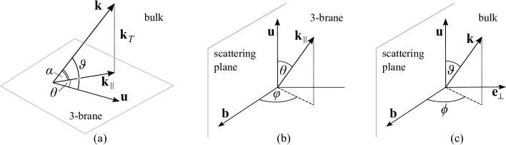
Introducing the angles according to Fig. 1 (for additional info see Appendix A), the normalization factor reads $N=\gamma v\sin\vartheta(ku^{\prime})$ and the following products do not vanish: $(e_{1}b)$, $(e_{1}u)$ and $(e_{2}b)$, respectively. The values of these contractions are given by

$$\varepsilon_{1}\cdot b=-b\,\cos\vartheta\cos\phi\,,\qquad\qquad\varepsilon_{1}\cdot u=\gamma v\sin\vartheta\,,\qquad\qquad\varepsilon_{2}\cdot b=-b\,\sin\phi\,.$$ (2.41)

For the derivation, see GKST4 . Thus the ”bulk” polarizations do not contribute into radiation; thereby in addition, one can introduce chiral polarization vectors in a usual way as

$$\varepsilon_{\pm}^{M}=\frac{\varepsilon_{1}^{M}\pm i\varepsilon_{2}^{M}}{\sqrt{2}}\;.$$ (2.42)

To summarize this Section: the formula for emitted radiation (2.37) and the appropriate polarization states of massless $D$-dimensional photon are derived, and for the problem-at-hand only two polarizations given in the covariant form (2.38, 2.39), contribute into the total emitted energy, as it is proper in four dimensions.

The source of the emitted field is to be computed within the iteration scheme based on the perturbation theory over gravitational constant $\varkappa_{D}$.

Notice, $J^{M}$ in (2.37) represents the total source of the total $A^{M}$ as a solution in flat space-time, and thus in our iteration scheme it is given by the series

$$J^{M}(k)=\,^{0}J^{M}(k)+j^{M}(k)+\ldots\,.$$ (2.43)

Here the $\,{}^{0}J^{M}$ given by (2.14) is a source of boosted Coulomb field, and its square does not contribute to the radiation. It will be shown below that the contribution of product $\,{}^{0}J^{*}\cdot j+\,^{0}J\cdot j^{*}$ also vanishes, and $\sum|j\cdot\varepsilon_{i}|^{2}$ becomes the first surviving order which contributes to the total emitted energy.

Thereby $j^{M}(k)$ (2.30) as well as its constituents becomes of particular significance and we concentrate on its evaluation. Looking at $\sigma^{M}(k)$ (2.32), it is enough to restrict ourselves on the first-order perturbation of the gravitational field $\,{}^{1}\!h^{MN}=\,^{1}\!h_{\rm m}^{MN}+\,^{1}\!h_{\rm m^{\prime}}^{MN}$. Thus in order to simplify notations, we keep $h^{MN}$ as a simplified notation of $\,{}^{1}\!h^{MN}_{\rm m}$ and denote, respectively, $h^{\prime MN}\equiv\,^{1}\!h^{MN}_{\rm m^{\prime}}$.

3 The radiation amplitudes

The first-order fields discussed above in the momentum space are given by

$$h_{MN}(q)=\frac{2\pi\hskip 1.00006pt\varkappa_{D}\hskip 1.00006ptm}{q^{2}}\,{\rm e}^{iqb}\,\delta(qu)\left(u_{M}u_{N}-\frac{1}{d+2}\,\eta_{MN}\right)\, \,{}^{1}\!A^{M}(q)=-\frac{2\pi\,e}{q^{2}}\,{\rm e}^{iqb}\,\delta(qu)\,u^{M}\,,$$ (3.1)

$$h^{\prime}_{MN}(q)=\frac{2\pi\varkappa_{D}m^{\prime}}{q^{2}}\,\delta(qu^{\prime})\left(u^{\prime}_{M}u^{\prime}_{N}-\frac{1}{d+2}\,\eta_{MN}\right)\, \,{}^{1}\!F^{MN}(q)=i\,\frac{2\pi\,e}{q^{2}}\,{\rm e}^{iqb}\,\delta(qu)\left[\hskip 0.59998ptq^{M}u^{N}-q^{N}u^{M}\vphantom{\frac{a}{a}}\right]\hskip 0.59998pt.$$

Respectively, the Fourier-transform of $\,{}^{0}\tilde{J}(x)=\,^{0}{J}(x)$ reads

$$\,^{0}{J}^{M}(q)=2\pi\,e\,{\rm e}^{iqb}\,\delta(qu)\,u^{M}\,.$$ (3.2)

Now we proceed to compute the two parts of the radiation amplitude.

3.1 Local amplitude

The Fourier transform of (2.31) reads

$$\rho^{M}(k)=e\,{\rm e}^{i(kb)}\!\int\!\left[\vphantom{\frac{a}{a}}{}^{1}\dot{z}^{M}+i\hskip 1.00006pt(k\,^{1}\!{z})\,u^{M}\right]{\rm e}^{i(ku)\tau}\,d\tau\,.$$ (3.3)

The first order correction to the trajectory is computed in GKST3 and we quote that result here.

$$\,^{1}\!z^{M}(\tau)=-\frac{im^{\prime}\varkappa_{D}^{2}}{(2\pi)^{D-1}}\int d^{\hskip 0.70004ptD}q\,\frac{\delta(qu^{\prime})}{q^{2}(qu)}\,{\rm e}^{-iqb}\left({\rm e}^{-i(qu)\tau}-1\right)\left[\gamma u^{\prime M}-\frac{1}{d+2}\,u^{M}-\frac{\gamma_{*}^{2}}{2\hskip 1.00006pt(qu)}\,q^{M}\right],$$ (3.4)

where $\gamma_{*}^{2}\equiv\gamma^{2}-{(d+2)}^{-1}$. We drop all the terms containing ${u^{\prime}}^{M}$ since they are transverse to the polarization vectors and thus will not contribute to the radiation. After integrating with respect to $\tau$ we obtain

$$\rho^{\hskip 0.41998ptM}(k)=-\frac{em^{\prime}\varkappa_{D}^{2}\,{\rm e}^{i(kb)}}{\left(2\pi\right)^{D-2}}\left[\,\gamma\hskip 1.00006ptI\left({u^{\prime}}^{M}-\frac{ku^{\prime}}{ku}\,\hskip 1.00006ptu^{M}\right)-\frac{\gamma_{*}^{2}}{2\hskip 1.00006pt(ku)}\,{I}^{M}+\frac{\gamma_{*}^{2}\,k\cdot{I}}{2\hskip 1.00006pt(ku)^{2}}\,u^{M}\,\right]\,,$$ (3.5)

where the integrals $I$ and $I^{M}$ are defined by

$$I=\int\frac{\delta(pu^{\prime})\,\delta(ku-pu)\,{\rm e}^{-i(pb)}}{p^{2}}\>d^{\hskip 0.70004ptD}p\,,\qquad\qquad I^{M}=\int\frac{\delta(pu^{\prime})\,\delta(ku-pu)\,{\rm e}^{-i(pb)}}{p^{2}}\;p^{\,M}\,d^{\hskip 0.70004ptD}p\,.$$ (3.6)

These integrals have been computed in GKST2 in terms of Macdonald functions (modified Bessel functions of 3rd kind):

$$I=-\frac{(2\pi)^{d/2+1}}{\gamma v\,b^{\hskip 0.70004ptd}}\,{\hat{K}}_{d/2}(z)\,,\qquad\qquad I^{M}=-\frac{(2\pi)^{d/2+1}}{\gamma v\hskip 1.00006ptb^{\hskip 0.70004ptd+2}}\left(b\hskip 1.00006ptz\hskip 1.00006pt{\hat{K}}_{d/2}(z)\,\frac{\gamma u^{\prime M}-u^{M}}{\gamma v}+i\hat{K}_{d/2+1}(z)\,b^{\hskip 0.41998ptM}\right),$$ (3.7)

with

$$z\equiv\frac{(ku)b}{\gamma v}\,,\qquad\qquad z^{\prime}\equiv\frac{(ku^{\prime})b}{\gamma v}\,,$$ (3.8)

where we use the more economic, non-conventional notation $\hat{K}_{\nu}(x)\equiv x^{\nu}{K}_{\nu}(x)$, in order to simplify the explanation of estimates making use of slowly altering at $[\hskip 0.59998pt0,\mathcal{O}\hskip 0.59998pt(1)\hskip 0.59998pt]$ function.

Substituting (3.7) into (3.5) one obtains

$$\rho^{\hskip 0.41998ptM}(k)=\frac{\lambda\,{\rm e}^{i(kb)}}{v}\left[\left(1-\frac{\gamma_{*}^{2}}{2\hskip 1.00006pt\gamma^{2}v^{2}}\right)\!\!\left(u^{\prime M}-\frac{z^{\prime}}{z}\,u^{M}\right)\hat{K}_{d/2}(z)+\frac{i\gamma_{*}^{2}}{2\hskip 1.00006pt\gamma^{2}v\hskip 0.59998ptz}\left(\frac{(kb)}{\gamma vz}\,u^{M}-\frac{b^{\hskip 0.41998ptM}}{b}\right)\hat{K}_{d/2+1}(z)\right],$$ (3.9)

with

$$\lambda\equiv\frac{e\hskip 1.00006ptm^{\prime}\hskip 0.59998pt\varkappa_{D}^{2}}{\left(2\pi\right)^{d/2+1}b^{\hskip 0.70004ptd}}\;.$$ (3.10)

Here we have restored the dependence on $u^{\prime M}$ in order to make obvious the conservation of the current (Subsection 3.5).

The local current $\rho^{M}(k)$ contains Macdonald functions $K_{\nu}(z)$ and, combined with the volume factor $\omega^{\hskip 0.41998ptd+2}\sin^{d+1}\vartheta$, gives dominant contribution in the region $\omega\sim\gamma^{2}\!/\hskip 0.59998ptb$, $\vartheta\sim\gamma^{-1}$ (i.e. $z\sim 1$), as was argued in GKST2 and will be discussed later in Subsection 5.1. In this region for the usage below we expand $\rho^{M}(k)$ in powers of $\gamma$:

$$\rho^{\hskip 0.41998ptM}(k)=\frac{\lambda\,{\rm e}^{i(kb)}}{2}\left[-\frac{z^{\prime}}{z}\,\hat{K}_{d/2}(z)\,u^{M}-i\left(\frac{z^{\prime}\sin\vartheta\cos\phi}{z}\,u^{M}+\frac{b^{\hskip 0.41998ptM}}{b}\right)\frac{\hat{K}_{d/2+1}(z)}{z}+\frac{d+1}{d+2}\,\frac{z^{\prime}}{\gamma^{2}z}\,\hat{K}_{d/2}(z)\,u^{M}+\mathcal{O}\hskip 0.59998pt(\gamma^{-2})\right]\!,$$ (3.11)

where the first term in the parenthesis is of order $\mathcal{O}\hskip 0.59998pt(\gamma)$, the square-bracket-term has order $\mathcal{O}\hskip 0.59998pt(1)$, while the last term is of order $\mathcal{O}\hskip 0.59998pt(\gamma^{-1})$ and the rest represents all subleading terms.

3.2 Non-local (stress) amplitude

The Fourier transform of (2.32) is given by

$$\sigma^{M}(k)=\frac{\varkappa_{D}^{2}\hskip 1.00006pte\hskip 1.00006ptm^{\prime}\,{\rm e}^{i\left(kb\right)}}{(2\pi)^{2}} \left[(ku^{\prime})\left((ku^{\prime})\,u^{M}-(ku)\,u^{\prime M}\vphantom{\frac{a}{a}}\right)J+\left(\gamma\left(ku^{\prime}\right)-\frac{\left(ku\right)}{d+2}\right)J^{M}+\right.$$

$$\quad+\left.\left(\frac{u^{M}}{d+2}-\gamma u^{\prime M}\right)k\cdot J+\left(\vphantom{\frac{a}{a}}(ku)\,u^{\prime M}-(ku^{\prime})\,u^{M}\right)u^{\prime}\cdot J\vphantom{\frac{a}{a}}\right]\,,$$ (3.12)

where

$$J(k)\equiv\int\frac{\delta(pu^{\prime})\,\delta(ku-pu)\,{\rm e}^{-i(pb)}}{p^{\hskip 0.70004pt2}\,(k-p)^{2}}\>d^{\hskip 0.70004ptD}p\,\,,\qquad\qquad J^{M}(k)\equiv\int\frac{\delta(pu^{\prime})\,\delta(ku-pu)\,{\rm e}^{-i(pb)}}{p^{\hskip 0.70004pt2}\,(k-p)^{2}}\,p^{M}\,d^{\hskip 0.70004ptD}p\,,$$ (3.13)

which have been computed in GKST4 as integrals over Feynman parameter $x$. We keep (3.2) for the proof of gauge conservation and further suppress terms proportional to ${u^{\prime}}^{M}$, as they do not contribute to the radiation. From this definition (3.13) it follows that $u^{\prime}\cdot J=0$, thus $\sigma^{M}(k)$ reads:

$$\sigma^{M}(k)=\frac{\lambda\,{\rm e}^{i\left(kb\right)}}{2\gamma v}\int\limits_{0}^{1}dx\,{\rm e}^{-i(kb)\,x} \left\{\left[\frac{\beta-x\xi^{2}}{d+2}-\left(\gamma z^{\prime}-\frac{z}{d+2}\right)\left((1-x)\,z+\gamma z^{\prime}x\vphantom{\frac{a}{a}}\right)+\gamma^{2}v^{2}{z^{\prime}}^{2}\right]\hat{K}_{d/2-1}(\zeta)\,u^{M}+\right.$$

$$\,\,\left.+\hskip 1.00006pti\hskip 1.00006pt\left[\frac{(kb)}{d+2}\,u^{M}+\left(\gamma^{2}vz^{\prime}-\frac{\gamma zv}{d+2}\right)\!\frac{b^{\hskip 0.41998ptM}}{b}\right]\hat{K}_{d/2}(\zeta)\right\},$$ (3.14)

with

$$\xi^{2}\equiv 2\hskip 1.00006pt\gamma\hskip 0.59998ptz\hskip 0.59998ptz^{\prime}-z^{2}-{z^{\prime}}^{2}\,,\qquad\qquad\beta\equiv\gamma\hskip 0.59998ptz\hskip 0.59998ptz^{\prime}-z^{2}\,,\qquad\qquad\zeta^{2}(x)\equiv{z^{\prime}}^{2}x^{2}+2\hskip 1.00006pt\gamma\hskip 0.59998ptz\hskip 0.59998ptz^{\prime}\hskip 0.59998ptx\left(1-x\right)+z^{2}\left(1-x\right)^{2}.$$

The non-local amplitude has now been written in terms of three scalar integrals of the following type:

$$J_{(\sigma,\tau)}\equiv\int\limits_{0}^{1}x^{\sigma}\,{\rm e}^{-i\left(kb\right)x}\,\hat{K}_{d/2+\tau}(\zeta)\,dx\,,\qquad\qquad(\sigma,\tau)=(0,-1),(0,0)\,\text{ and }\,(1,-1)\,.$$ (3.15)

These integrals have been studied in details in GKST4 : introducing parameter $\varrho\sim\omega\hskip 0.59998ptb\hskip 1.00006pt\vartheta$, (3.15) is expanded as series over $1/\varrho$. Thus in the high-frequency region (or $z-$region, for brevity) $\omega\sim\gamma^{2}\!/\hskip 0.59998ptb$, $\vartheta\sim\gamma^{-1}$ the dominant contribution comes from small $x=0\ldots\mathcal{O}\hskip 0.59998pt(\gamma^{-2})$ and all integrals (3.15) are to be expanded in terms of Macdonald functions with argument $\zeta(0)=z$, with expansion parameter $1/\gamma$. In the large-angle region (or $z^{\prime}-$region) $\omega\sim\gamma/\hskip 0.59998ptb$, $\vartheta\sim 1$ the dominant contribution comes from the values of $x$ near 1: $x=1-\mathcal{O}\hskip 0.59998pt(\gamma^{-2})\ldots 1$ and all such integrals are to be expanded in terms of Macdonald functions with argument $\zeta(1)=z^{\prime}$.

In the transition region ($\omega\sim\gamma/\hskip 0.59998ptb$, $\vartheta\sim\gamma^{-1}$) the exponential in (3.2) does not oscillate rapidly and the whole domain $x=[0,1]$ contributes equally. The series with Macdonald functions $K_{\nu}(z)$ and $K_{\nu^{\prime}}(z^{\prime})$ is also valid (see Appendix C) but converges very slow since no small factor is available. Finally, in the ultimate region ($\omega\sim\gamma^{2}\!/\hskip 0.59998ptb$, $\vartheta\sim 1$) the whole integral is exponentially suppressed by $\mathcal{O}\hskip 0.59998pt({\rm e}^{\gamma})$.

Next we consider more thoroughly the high-frequency behavior of local and non-local amplitudes.

3.3 Destructive interference

We now proceed to demonstrate the cancelation of the two leading orders of $\sigma^{M}$ and $\rho^{M}$ in powers of $\gamma$ in the $z-$region, which leads to the strong damp of the amplitude by $\mathcal{O}\hskip 0.59998pt(\gamma^{2})$ and the emitted energy by four orders of $\gamma$. We will refer to this effect as destructive interference. The same effect for gravity was described in GKST3 ; GKST4 by means of the same representation via Macdonald functions. In another representation it appeared in ggm dealing with only four dimensions.

We follow GKST4 and sketch the procedure for showing this: in the $z-$region ($z\sim 1,z^{\prime}\sim\gamma$) the integral $J_{(1,-1)}$ is suppressed by two orders of $\gamma$ with respect to the $J_{(0,-1)}$ and $J_{(0,0)}$ as it was implicitly mentioned in the previous Subsection and proved in (GKST4, , eqn.(3.28)). We now keep only the terms that will give us the first three orders of (3.2):

$$\sigma^{M}(k)\approx\frac{\lambda\,{\rm e}^{i(kb)}z^{\prime}\gamma}{2}\int\limits_{0}^{1}dx\,{\rm e}^{-i(kb)\,x}\left[{z^{\prime}}\hat{K}_{d/2-1}(\zeta)\,u^{M}+\frac{i}{b}\,\hat{K}_{d/2}\left(\zeta\right)\,b^{\hskip 0.41998ptM}-\left(\frac{d+1}{d+2}\,\frac{z}{\gamma}+\frac{{z^{\prime}}}{\gamma^{2}}+z^{\prime}x\right)\hat{K}_{d/2-1}(\zeta)\,u^{M}\right].$$ (3.16)

Finally we substitute the approximation (GKST4, , eqn.(B.10)), appropriately simplified here neglecting the exponentially suppressed Macdonalds $K_{\nu^{\prime}}(z^{\prime})$ ($a\equiv{z}/{\sin\vartheta}$):

$$\,\,\,\int\limits^{1}_{0}\!dx\,{\rm e}^{-i(kb)\hskip 0.70004ptx}\hat{K}_{\nu-1}(\zeta) \approx\frac{\beta}{a^{2}\xi^{2}}\left(\hat{K}_{\nu}(z)-i\frac{(kb)}{\beta}\,\hat{K}_{\nu+1}(z)-\frac{2\nu+1}{a^{2}}\,\hat{K}_{\nu+1}(z)+\frac{\sin^{2}\!\phi}{a^{2}}\,\hat{K}_{\nu+2}(z)\right)+\ldots$$ (3.17)

$$\approx\frac{\hat{K}_{\nu}(z)}{\gamma zz^{\prime}}-i\frac{(kb)\,\hat{K}_{\nu+1}(z)}{(\gamma zz)^{2}}+\frac{1-\gamma^{2}\psi}{\gamma^{3}z^{\prime}z}\,\hat{K}_{\nu}(z)-\frac{\sin^{2}\!\vartheta}{\gamma z^{3}z^{\prime}}\left[(2\nu+1)\hat{K}_{\nu+1}(z)-\sin^{2}\!\phi\,\hat{K}_{\nu+2}(z)\right].$$

For $J_{(1,-1)}$-type integral (GKST4, , eqn.(3.28)) we retain only the leading terms:

$$\int\limits^{1}_{0}dx\,x\,{\rm e}^{-i(kb)\hskip 0.70004ptx}\hat{K}_{\nu-1}(\zeta)\approx-\frac{1}{\left(\gamma z^{\prime}\right)^{2}}\,\hat{K}_{\nu}(z)-\frac{\left(2\nu+1\right)}{\left(\gamma zz^{\prime}\right)^{2}}\,\hat{K}_{\nu+1}(z)+\frac{1}{\left(\gamma zz^{\prime}\right)^{2}}\,\hat{K}_{\nu+2}(z)\,.$$

Thus upon substitution of the latter two into (3.16) and retaining the first three orders, one obtains:

$$\sigma^{M}\approx\frac{\lambda\,{\rm e}^{i\left(kb\right)}}{2\gamma} \left[\frac{\gamma z^{\prime}}{z}\,\hat{K}_{d/2}\left(z\right)u^{M}+i\left(\gamma\frac{b^{\hskip 0.41998ptM}}{b}-\frac{\left(kb\right)}{z}u^{M}\right)\frac{\hat{K}_{d/2+1}(z)}{z}\,-\frac{d+1}{d+2}\,\hat{K}_{d/2}(z)\,u^{M}-\right.$$ (3.18)

$$\;\left.-(d+1)\left(1-\frac{\sin^{2}\!\vartheta}{\psi}\right)\frac{\hat{K}_{d/2+1}(z)}{z^{2}}\,u^{M}+\left(\!\left(\frac{\sin^{2}\!\vartheta\sin^{2}\!\phi}{\psi}-1\right)u^{M}+\frac{(kb)}{z^{\prime}}\frac{b^{\hskip 0.41998ptM}}{b}\right)\frac{\hat{K}_{d/2+2}(z)}{z^{2}}\right].$$

The first two orders of this expression exactly cancel with the first two orders of (3.11), leaving us with

$$j^{M}\approx\frac{\lambda\,{\rm e}^{i\left(kb\right)}}{2\gamma}\left[\frac{d+1}{d+2}\,\left(\frac{1}{\gamma^{2}\psi}-1\right)\hat{K}_{d/2}(z)\,u^{M}-(d+1)\left(1-\frac{\sin^{2}\!\vartheta}{\psi}\right)\frac{\hat{K}_{d/2+1}(z)}{z^{2}}\,u^{M}\right.+$$

$$\left.+\left(\!\left(\frac{\sin^{2}\!\vartheta\sin^{2}\!\phi}{\psi}-1\right)u^{M}+\frac{(kb)}{z^{\prime}}\frac{b^{\hskip 0.41998ptM}}{b}\right)\frac{\hat{K}_{d/2+2}(z)}{z^{2}}\right].$$ (3.19)

We note that even though the current will finally be projected on the two polarization vectors, this will not change our conclusion, as the contractions (2.41) add no powers of $\gamma$ at the region of interest.

3.4 The total radiation amplitude

In order to compute the total radiation energy, we will need to study the following three regions. The $z$-type radiation emitted for angles $\vartheta\sim 1/\gamma$ and $\omega\sim\gamma^{2}\!/\hskip 0.59998ptb$, the region with frequency $\omega\sim\gamma/\hskip 0.59998ptb$ again for small angles and finally the radiation at angles $\vartheta\sim 1$ at medium-frequencies.

High frequency regime. The radiation amplitude in $z-$regime after the destructive interference was derived in the previous Subsection. Projecting (3.3) on (2.42), the chiral amplitudes $j_{\pm}\equiv j\cdot\varepsilon_{\pm}$ read:

$$j_{\pm}(k)\approx\frac{\lambda\,{\rm e}^{i(kb)}\sin\vartheta}{2\sqrt{2}} \left[\frac{d+1}{d+2}\,\frac{1-\gamma^{2}\psi}{\gamma^{2}\psi}\,\hat{K}_{d/2}(z)-\frac{d+1}{z^{2}}\left(\frac{\sin^{2}\!\vartheta}{\psi}-1\right)\hat{K}_{d/2+1}(z)+\right.$$

$$\;\;\left.+\frac{\sin^{2}\!\phi}{z^{2}}\left(\frac{\sin^{2}\!\vartheta}{\psi}-1\right)\hat{K}_{d/2+2}(z)\pm i\,\frac{\sin 2\phi}{2\,z^{2}}\,\hat{K}_{d/2+2}(z)\right].$$ (3.20)

All terms in the parenthesis (3.4) are of order ${\mathcal{O}\hskip 0.59998pt(1)}$ (in $\lambda=1$ units) within $z-$regime, hence the whole amplitude goes like $\mathcal{O}\hskip 0.59998pt(\gamma^{-1})$ due to the common pre-factor $\sin\vartheta$.

Large angle regime. In this region of the parameters ($z^{\prime}-$regime) $z$ is of order $\mathcal{O}\hskip 0.59998pt(\gamma)$, so the Macdonald functions that have $z$ as their argument are exponentially suppressed. Thus we ignore the local part of the current and consider only the non-local part. To repeat, in this regime the main contribution of the integrals with respect to $x$ comes from the area near $x=1$, and the integrals $J_{0,\tau}-J_{1,\tau}$, which are of the form $1-x$, are suppressed by a factor of $\mathcal{O}\hskip 0.59998pt(\gamma^{-2})$ with respect to both $J_{0,\tau}$ and $J_{1,\tau}$. We rewrite (3.2) in a way where we are expanding both with respect to $\gamma$ but also with respect to $1-x$. Taking also into account that $u^{M}$ is perpendicular to the second projection, while it gives us an order of $\gamma$ when projected on the first polarization, while $b^{\hskip 0.41998ptM}$ gives no additional powers of $\gamma$ when projected on either polarization, we write the two leading orders:

$$j^{M}(k)\approx\frac{\lambda\,{\rm e}^{i\left(kb\right)}}{2\gamma}\int\limits_{0}^{1}dx\,{\rm e}^{-i(kb)\hskip 0.70004ptx} \left\{\left[\!\vphantom{\frac{d}{d}}\right.\right.\!\!\left(\gamma^{2}{z^{\prime}}^{2}-\frac{d+1}{d+2}\,\gamma zz^{\prime}\right)(1-x)+\frac{{z^{\prime}}^{2}}{d+2}\left.\vphantom{\frac{d}{d}}\right]\hat{K}_{d/2-1}(\zeta)\,u^{M}$$

$$\,\,\left.+\,i\hskip 1.00006pt\left[\frac{(kb)}{d+2}\,u^{M}+\left(\gamma^{2}z^{\prime}-\frac{\gamma z}{d+2}\right)\frac{b^{\hskip 0.41998ptM}}{b}\right]\hat{K}_{d/2}\left(\zeta\right)\right\}\,.$$ (3.21)

Since no destructive interference is expected, we retain only the leading terms of integrals, and set $x=1$ inside the integrand of (3.4). These integrals have been computed in GKST4 and give, to the leading order,

$$\int\limits^{1}_{0}{\rm e}^{i\left(kb\right)x}\,\hat{K}_{\tau}(\zeta)\,dx\approx\,\frac{{\rm e}^{-i\left(kb\right)}}{{z^{\prime}}^{2}\gamma^{2}\psi}\,\hat{K}_{\tau+1}(z^{\prime})\,.$$ (3.22)

Eventually, the entire first line in (3.4) turns out to be subleading with respect to the second one, and, upon substitution (3.22) $j^{M}$ reads:

$$j^{M}(k)\approx\frac{\lambda\,i}{2\gamma\psi}\left[\frac{(kb)}{\gamma^{2}{z^{\prime}}^{2}(d+2)}\,u^{M}+\left(\frac{1}{z^{\prime}}-\frac{z}{\gamma z^{\prime}(d+2)}\right)\frac{b^{\hskip 0.41998ptM}}{b}\right]\hat{K}_{d/2+1}(z^{\prime})\,.$$ (3.23)

Finally projecting on $\varepsilon_{\pm}$ (2.42) the two significant radiation amplitudes in $z^{\prime}-$region are given by

$$j_{\pm}(k)\approx\frac{\lambda\,i}{2\sqrt{2}\hskip 1.00006pt\gamma\hskip 1.00006pt\psi}\left[-\frac{\sin^{2}\vartheta\,\cos\phi}{{z^{\prime}}(d+2)}\,+\left(\frac{\psi}{d+2}-\frac{1}{z^{\prime}}\right)\cos\vartheta\cos\phi\pm i\left(\frac{\psi}{d+2}-\frac{1}{z^{\prime}}\right)\sin\phi\right]\hat{K}_{d/2+1}(z^{\prime})\,.$$ (3.24)

In what follows, the amplitudes are of order $\mathcal{O}\hskip 0.59998pt(\gamma^{-1})$.

Transition regime. In this region, the projection of the current on the polarization vectors will once more not add any powers of $\gamma$. We have $z\sim 1/\gamma$ and $z^{\prime}\sim 1$. Looking at expressions (3.9) and (3.2) we see that they are of the same order $\mathcal{O}\hskip 0.59998pt(\gamma)$ in any dimension in units $\lambda=1$.

3.5 Conservation of current and validity of gauge fixation

In the above analysis, the following gauges were fixed:

• the affine parametrization of the trajectories along the worldlines of the scattered particles:

  $$g_{MN}\dot{z}^{M}\dot{z}^{N}=g_{MN}\left.\dot{z}^{\hskip 0.41998pt\prime}\right.^{M}\!\left.\dot{z}^{\hskip 0.41998pt\prime}\right.^{N}=1\,;$$ (3.25)

• the de Donder gauge on the gravitational field:

  $$\partial_{M}\,{}^{k}\psi^{MN}=0,\qquad\qquad k=1,2,\ldots\,;$$ (3.26)

• the Lorentz gauge on the vector field:

  $$\partial_{M}\,{}^{k}A^{M}=0,\qquad\qquad k=1,2,\ldots\,.$$ (3.27)

To verify self-consistency of our scheme (at least to the lowest orders of interest), we show it explicitly.

To zeroth order, (3.25) degenerates into $u^{2}=1$ and ${u^{\prime}}^{2}=1$ which is trivially satisfied.

In the first order, variation of (3.25) reads

$$\varkappa_{D}h^{\prime}_{MN}(\,^{0}z)\,u^{M}u^{N}+2\,(\,^{1}\!\dot{z}\cdot u)=0\,,\qquad\qquad\varkappa_{D}h_{MN}(\,^{0}z^{\prime})\,{u^{\prime}}^{M}{u^{\prime}}^{N}+2\,(\,^{1}\!\left.\dot{z}^{\hskip 0.41998pt\prime}\right.\cdot u^{\prime})=0\,,$$ (3.28)

respectively. From (3.1) the value of $h^{\prime}_{MN}(x)$ at the location of $m-$particle $x=\,^{0}z(\tau)$ reads

$$h_{MN}(\,^{0}z)=\frac{\varkappa_{D}\hskip 1.00006ptm^{\prime}}{(2\pi)^{D-1}}\int d^{\hskip 0.70004ptD}q\frac{\delta(qu^{\prime})}{q^{2}}\left(u^{\prime}_{M}u^{\prime}_{N}-\frac{1}{d+2}\,\eta_{MN}\right)\,{\rm e}^{-iqz_{0}}.$$ (3.29)

Contracting it with $u^{M}\hskip 1.00006ptu^{N}$ and substituting $\,{}^{0}z^{M}(\tau)=u^{M}\hskip 1.00006pt\tau+b^{\hskip 0.41998ptM}$ one obtains

$$h_{MN}(\,^{0}z)\,u^{M}\hskip 1.00006ptu^{N}=\frac{\varkappa_{D}\hskip 1.00006ptm^{\prime}}{(2\pi)^{D-1}}\int d^{\hskip 0.70004ptD}q\frac{\delta(qu^{\prime})}{q^{2}}\left(\gamma^{2}-\frac{1}{d+2}\right)\,{\rm e}^{-iq\hskip 0.70004pt\cdot(u\tau+b)}.$$ (3.30)

Differentiating (3.4) and contracting with $u^{M}$ one obtains

$$\left(\,{}^{1}\!\dot{z}(\tau)\cdot u\right)=-\frac{m^{\prime}\varkappa_{D}^{2}\,\gamma_{*}^{2}}{2(2\pi)^{D-1}}\int d^{\hskip 0.70004ptD}q\,\frac{\delta(qu^{\prime})}{q^{2}}\,{\rm e}^{-iqb}\,{\rm e}^{-i\hskip 0.41998pt(qu)\hskip 0.41998pt\tau}\,.$$ (3.31)

Multiplying it by 2 and combining with (3.30) one gets the cancelation and thereby verifies (3.28) to the first order. The gauge on the trajectory of $m^{\prime}-$particle is checked similarly.

Next, proceeding to the de Donder gauge on $\,{}^{1}\!\psi_{MN}$: one rewrites (3.1):

$$\,{}^{1}\!\psi^{MN}(q)=\frac{2\pi\,\varkappa_{D}\hskip 1.00006ptm}{q^{2}}\,{\rm e}^{iqb}\,\delta(qu)\,u^{M}u^{N}\,.$$

The divergence in Fourier space reads

$$q_{N}\,^{1}\!\psi^{MN}(q)=\frac{2\pi\,\varkappa_{D}\hskip 1.00006ptm}{q^{2}}\,{\rm e}^{iqb}\,(qu)\,\delta(qu)\,u^{M}=0\,,$$

by virtue of distributional identity $x\,\delta(x)=0$.

The divergence of $\,{}^{1}\!A^{M}$ (the first order of (3.27)) vanishes due to the same reason:

$$q_{M}\,^{1}\!A^{M}(q)=-\frac{2\pi\,e}{q^{2}}\,{\rm e}^{iqb}\,\delta(qu)\,(qu)=0\,.$$ (3.32)

Let also verify the gauge on $\,{}^{2}\!A^{M}$: in the momentum space

$$\,{}^{2}\!A^{M}(k)=-\frac{\,{}^{2}\!j^{M}(k)}{k^{2}}\,,$$

where $j^{M}(k)$ is the full Fourier-transform taken off-shell $k^{2}=0$ and with no terms neglected due to polarizations. Thus Lorentz gauge of $\,{}^{2}\!A^{M}$ is equivalent to $k\cdot j=0$.

The constituents of $j^{M}(k)$ are given by (3.5,3.9) and (3.2). Projecting both on $k^{M}$ one concludes $k\cdot\rho(k)=0$ and $k\cdot\sigma(k)=0$. Thus both

$$\partial_{M}\hskip 1.00006pt\rho^{M}(x)=0\,,\qquad\qquad\partial_{M}\hskip 1.00006pt\sigma^{M}(x)=0$$

conserve separately, as well as their sum.

Finally, one has to point out, that the conservation of $\,{}^{2}\!A^{M}$ on flat background represents the same effect as conservation of $J^{M}$ (2.4) (continuity equation) in the curved background:

$$\nabla_{M}J^{M}(x)=0\,.$$ (3.33)

Explicitly the latter reads

$$\nabla_{M}{J^{M}}=\partial_{M}J^{M}+\Gamma^{N}_{N,M}\hskip 1.00006ptJ^{M}\,.$$ (3.34)

The zeroth-order variation coincides with the conservation of $\,{}^{0}J^{M}=\,^{0}\tilde{J}^{M}$ discussed above. The first-order variation of (3.34) is given by

$$\,^{1}\!\left[\nabla_{M}{J^{M}}\right]=\partial_{M}\,^{1}\!J^{M}+\,^{1}\!\hskip 1.00006pt\Gamma^{N}_{N,M}\,{}^{0}J^{M}\,.$$ (3.35)

These terms read

$$\partial_{M}\,^{1}\!{J^{M}}=e\,\partial_{M}\int\left(\,{}^{1}\!\dot{z}^{M}-u^{M}\,{}^{1}\!z^{N}\partial_{N}-\frac{\varkappa_{D}}{2}\,h\,u^{M}\right)\delta^{D}\!\left(x-\,^{0}z\right)\,d\tau\,$$

$$\,{}^{1}\!\hskip 1.00006pt\Gamma^{N}_{N,M}\,{}^{0}J^{M}=\frac{e\hskip 1.00006pt\varkappa_{D}}{2}\,h_{,M}\int u^{M}\,\delta^{D}\!\left(x-\,^{0}z\right)\,d\tau\,,$$ (3.36)

thus their sum equals

$$e\,\int\left(\,{}^{1}\!\dot{z}^{M}-u^{M}\,{}^{1}\!z^{N}\partial_{N}\right)\partial_{M}\,\delta^{D}\!\left(x-\,^{0}z\right)\,d\tau=e\int d\left(\vphantom{\frac{a}{a}}\,{}^{1}\!z^{M}\,\partial_{M}\,\delta^{D}\!\left(x-\,^{0}z\right)\right)=0$$ (3.37)

as a total derivative. The latter represents the proof in coordinate-space of the property $\partial_{M}\hskip 1.00006pt\,^{1}\!\tilde{J}^{M}(x)=\partial_{M}\hskip 1.00006pt\rho^{M}(x)=0$, discussed above.

Thus the iteration scheme we use is compatible with the gauge we fix, and gives the apparent way to compute radiation amplitude and, eventually, the flux of emitted momentum.

4 The emitted energy

In order to compute the emitted energy, we take the zeroth component of the emitted momentum (2.37):

$$E=\frac{1}{2\left(2\pi\right)^{d+3}}\sum_{i}\int\limits^{\infty}_{0}\omega^{d+2}d\omega\int d\Omega\;|j_{\hskip 0.70004pti}(k)|^{2},$$ (4.1)

First we summarize the radiation amplitudes derived in the previous Section and overview the corresponding contributions to the total flux. In Table I we present the energy emitted in the several relevant regimes of frequency and angle, where the estimates of contribution to the total emitted energy are deduced from (4.1) with the estimate of $j_{\hskip 0.70004pti}(k)$ and the characteristic value of $\vartheta$ and $\omega$ following immediately from the corresponding Table’s entry.

	$\omega\lesssim 1/\hskip 0.59998ptb$	$\omega\sim\gamma/\hskip 0.59998ptb$	$\omega\sim\gamma^{2}\!/\hskip 0.59998ptb$	$\omega\gg\gamma^{2}\!/\hskip 0.59998ptb$
$\gamma^{-1}$	$\begin{array}[]{c}\rule{0.0pt}{13.00005pt}j\sim\mathrm{Im}\rho\\ E_{\mathrm{rad}}\sim\gamma^{2}\\ \text{\footnotesize subleading by}\\ \text{\footnotesize(phase space)}\end{array}$	$\begin{array}[]{l}\rule{0.0pt}{13.00005pt}j\sim\mathcal{O}\hskip 0.59998pt(\gamma),\text{\footnotesize{} from }\rho\text{\footnotesize{} and }\sigma\\ x\in[0,1],\;\text{\footnotesize{} medium regime}\\ \text{ \footnotesize no destructive interference }\\ E_{\mathrm{rad}}\sim\gamma^{3}\\ \end{array}$	$\begin{array}[]{l}\rule{0.0pt}{13.00005pt}j\sim\mathcal{O}\hskip 0.59998pt(\gamma^{-1}),\text{\footnotesize{} from }\rho+\sigma(z)\\ x\in[0,\mathcal{O}\hskip 0.59998pt(\gamma^{-2})],\;z-\text{\footnotesize{}regime}\\ \text{\footnotesize destructive interference}\\ E_{\mathrm{rad}}\sim\gamma^{d+2}\end{array}$	$\begin{array}[]{c}\text{\footnotesize negligible radiation}\\ \text{\footnotesize exponential fall-off}\\ \end{array}$
1	$\begin{array}[]{c}j\sim\rho\\ E_{\mathrm{rad}}\sim 1\\ \text{\footnotesize(phase space)}\end{array}$	$\begin{array}[]{l}\rule{0.0pt}{13.00005pt}j\sim\mathcal{O}\hskip 0.59998pt(\gamma^{-1}),\text{\footnotesize{} from }\sigma(z^{\prime})\\ x\in[1-\mathcal{O}\hskip 0.59998pt(\gamma^{-2}),1]\\ z^{\prime}-\text{\footnotesize regime},\,E_{\mathrm{rad}}\sim\gamma^{d+1}\end{array}$	$\begin{array}[]{c}\text{\footnotesize negligible radiation}\\ \text{\footnotesize exponential fall-off}\\ \end{array}$	$\begin{array}[]{c}\text{\footnotesize negligible radiation}\\ \text{\footnotesize exponential fall-off}\\ \end{array}$

Table 1: The behavior of radiation amplitudes and contribution to the emitted energy of each of the several characteristic regions of angle and frequency. The values are normalized as $\lambda=b=1$.

Now we illustrate qualitatively the effects described above and based on the derivation in previous Section.

On Fig.2 we plot a characteristic picture of the behavior of local and non-local amplitudes and their sum (the radiation amplitude) for the case $d=0$ at characteristic value of $\vartheta$ and some common value of $\phi$.

Figure 2: Radiation amplitudes of first polarization for $d=0$ and $\gamma=10^{3}$ in logarithmic scales $x=\log_{\hskip 0.70004pt\gamma}\omega b$ and $y=\log_{\hskip 0.70004pt\gamma}|{\rm amplitude}|$, evaluated at $\vartheta=1/\gamma,\,\phi=\pi/4$. The plots are given for $-{\rm Re}\,\rho(k)$ (red, dashed), ${\rm Im}\,\rho(k)$ (green, dot-dashed), ${\rm Re}\,\sigma$ (black, dotted) and ${\rm Re}\,j$ (cyan, solid). At $x\approx 1$ the curve $\log_{\gamma}|{\rm Re}\,j|$ in logarithmic scale has discontinuity $y=-\infty$ related with the fact that corresponding original amplitude ${\rm Re}\,j$ changes its sign.

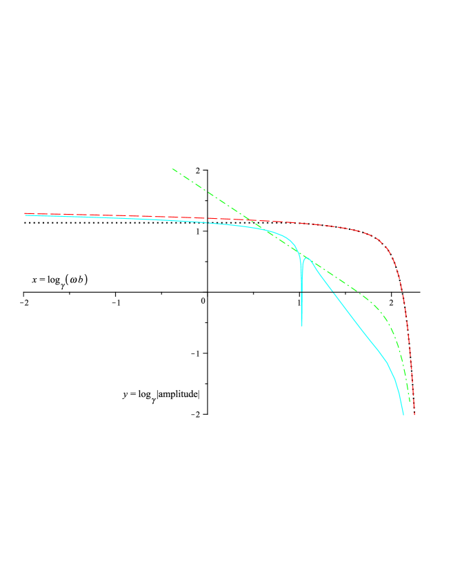
The qualitative features deserving attention are the following:

• At $\omega\to 0$ ${\rm Im}\,\rho(k)$ goes like $1/\omega$ and dominates in total $j$, in Fig. 2 it corresponds to the asymptote with tangent $-1$ on green (dot-dashed) curve. This property is valid for all $d\geqslant 0$ and will be of usage further, when the zero-frequency limit is to be computed;

• At $x\to-\infty$ ($\omega\to 0$) $|{\rm Re}\,\sigma|\ll|{\rm Re}\,\rho|$ hence ${\rm Re}\,j\approx{\rm Re}\,\rho$. At this limit $\omega\to 0$ $|{\rm Re}\,\sigma|$ goes like $\omega^{0}$ (black, dotted line in Fig. 2) for $d=0$, like $\omega^{1}$ for $d=1$ and like $\omega^{2}$ for $d\geqslant 2$, as it follows directly from (3.2) and behavior of hatted Macdonald functions.

• At $x>2$ each curve has rapid fall-off at $y=-\infty$, corresponding to the strong exponential decay of an amplitude at $\omega\gtrsim\gamma^{2}\!/\hskip 0.59998ptb$;

• At $x>1$ ${\rm Re}\,\sigma\approx-{\rm Re}\,\rho$, so their sum (difference of absolute values in the plot) ${\rm Re}\,j$ (cyan, solid) is much smaller. At $x\approx 2$ the difference of ${\rm Re}\,j$ and ${\rm Re}\,\rho$ is $\Delta y\approx 2$, so $j$ is damped by $\gamma^{2}$ with respect to ${\rm Re}\,\rho$. This illustrates the destructive interference at $\gamma^{2}\!/\hskip 0.59998ptb>\omega\gg\gamma/\hskip 0.59998ptb$, that can be rewritten as

  $$j(\omega)\sim j(\omega_{0})\,\frac{\omega_{0}^{2}}{\omega^{2}}\,,\qquad\qquad\omega_{0}\sim\frac{\gamma}{b}\,;$$

• In the region $x=(1,2)$ $\log_{\gamma}|{\rm Re}\,j|$ represents straight-line piece with tangent $-2$, what corresponds to the destructive interference region $\omega=(\gamma/\hskip 0.59998ptb,\gamma^{2}\!/\hskip 0.59998ptb)$. Thus the radiation amplitude itself goes like $\omega^{-2}$ at this region. Being averaged over angles (with some average angle $\bar{\vartheta}=\mathcal{O}\hskip 0.59998pt(\gamma^{-1})$), the same is valid for the frequency distribution. For higher dimensions the corresponding behavior of the latter ${dE}/{d\omega}\equiv F$ is

  $$F(\omega)\sim(\omega\bar{\vartheta})^{d+2}j^{2}(\omega)\sim\frac{j^{2}(\omega_{0})\,\omega_{0}^{4}\,}{\gamma^{d+2}}\,\omega^{d-2}\sim\gamma^{4-d}\,\omega^{d-2},\qquad\qquad\gamma/\hskip 0.59998ptb<\omega<\gamma^{2}\!/\hskip 0.59998ptb$$ (4.2)

  in this region;

• $|{\rm Im}\,\rho|$ is subleading with respect to $|{\rm Re}\,\sigma|$ but larger than $|{\rm Re}\,j|$ (at $x>1$) on this plot. It is damped by $|{\rm Im}\,\sigma|$ not presented here, so their sum $|{\rm Im}\,j|$ becomes much smaller than $|{\rm Re}\,j|$.

Thus in fact, we have two radiation amplitudes instead of a single one in GKST3 , with obvious identification $f\to e,f^{\prime}\to e^{\prime}$. In other words our primary problem now is to derive the final overall coefficient.

4.1 Total radiated energy

As can be seen from Table I, the dominant radiation comes from different regimes depending on the number of extra dimensions, $d$. Indeed, as it follows from (4.2),

$$E\sim\int\limits_{\sim\hskip 0.70004pt\gamma/\hskip 0.41998ptb}^{\sim\hskip 0.70004pt\gamma^{2}\!/\hskip 0.41998ptb}\frac{dE}{d\omega}\,d\omega\sim\frac{1}{\gamma^{d-4}}\int\limits_{\omega_{0}}^{\gamma\omega_{0}}\omega^{d-2}\,d\omega\,,$$ (4.3)

so the dominant contribution comes from the upper limit $\omega\sim\gamma^{2}\!/\hskip 0.59998ptb\hskip 1.00006pt$ for $d\geqslant 2$, from the lower limit $\omega_{0}\sim\gamma/\hskip 0.59998ptb$ for $d=0$ and from the whole domain for $d\geqslant 1$, respectively.

According to this argument, we need to consider separately the cases where the number of extra dimensions are $d=0$, $d=1$ and $d\geqslant 2$. We start with studying the $d\geqslant 2$ case.

$\boldsymbol{d}\mathbf{\geqslant 2.}$ In this case, as can be seen in the table, the radiation with frequency in the area of $\omega\sim\gamma^{2}\!/\hskip 0.59998ptb$ dominates. In the case of interest here, $R\gg b$, we can replace the summation by integration and use the uncompactified formula for the emitted energy.

The next step is to substitute the expression we have already found for (2.42), which will give the dominant contribution in this case. We notice that when squaring the two amplitudes we will have products of the Macdonald functions. In order to perform the integration over $\omega$, we will change variable to $z$ and the radiated energy will take the following form:

$$\frac{dE}{d\Omega}=\frac{\lambda^{2}\sin^{d+3}\vartheta}{8\left(2\pi\right)^{d+3}b^{\hskip 0.70004ptd+3}\psi^{d+3}}\sum_{a,b=0}^{2}C_{ab}^{(d\hskip 0.41998pt)}D_{ab}^{(d\hskip 0.41998pt)}(\vartheta,\phi)\,,$$ (4.4)

with $C_{ab}^{(d\hskip 0.41998pt)}\equiv\int\hat{K}_{d/2+a}(z)\hat{K}_{d/2+b}(z)\,z^{d+2\left(\delta_{0a}+\delta_{0b}-1\right)}\,dz$. We are now left with the integration over $\omega$. The expressions for $j_{\pm}(k)$ (3.4) are accurate for high frequencies, however it has been shown GKST3 that for $d\geqslant 2$ it is possible to expand the integration domain $z=(\sim 1/\gamma,\infty)$ up to $z=(0,\infty)$, with the relative error $\mathcal{O}\hskip 0.59998pt(\gamma^{-1})$. Computing $C_{ab}^{(d\hskip 0.41998pt)}$ with help of Proudn

$$\int\limits_{0}^{\infty}K_{\mu}(z)K_{\nu}(z)\,z^{\alpha-1}\hskip 1.00006ptdz=\frac{2^{\alpha-3}\Gamma\left(\frac{\alpha+\mu+\nu}{2}\right)\Gamma\left(\frac{\alpha+\mu-\nu}{2}\right)\Gamma\left(\frac{\alpha-\mu+\nu}{2}\right)\Gamma\left(\frac{\alpha-\mu-\nu}{2}\right)}{\Gamma\left(\alpha\right)}\,,\qquad\qquad\alpha>\mu+\nu$$ (4.5)

and summing up the contributions of two chiral polarizations, the angular part reads

$$D_{00}^{(d\hskip 0.41998pt)} =\left(\frac{d+1}{d+2}\right)^{\!2}\left(\frac{1}{\gamma^{4}\psi^{2}}-\frac{2}{\gamma^{2}\psi}+1\right)\,,\quad\quad D {}_{11}^{(d\hskip 0.41998pt)}=\left(d+1\right)^{2}\left(\frac{\sin^{2}\!\vartheta}{\psi}-1\right)^{\!2}\,,$$

$$D_{22}^{(d\hskip 0.41998pt)} =\sin^{4}\!\phi\left(\frac{\sin^{2}\!\vartheta}{\psi}-1\right)^{\!2}+\frac{\sin^{2}\!2\phi}{4}\;,\quad\quad D {}_{01}^{(d\hskip 0.41998pt)}=-\frac{\left(d+1\right)^{2}}{d+2}\left(\frac{\sin^{2}\!\vartheta}{\psi}-1\right)\frac{1-\gamma^{2}\psi}{\gamma^{2}\psi}\,,$$

$$D_{02}^{(d\hskip 0.41998pt)} =\frac{d+1}{d+2}\left(\frac{\sin^{2}\!\vartheta}{\psi}-1\right)\frac{1-\gamma^{2}\psi}{\gamma^{2}\psi}\,\sin^{2}\!\phi\;,\quad\quad D {}_{12}^{(d\hskip 0.41998pt)}=-\left(d+1\right)\left(\frac{\sin^{2}\!\vartheta}{\psi}-1\right)^{\!2}\sin^{2}\!\phi\;.$$ (4.6)

By virtue of summation, we can integrate each $D_{ab}^{(d\hskip 0.41998pt)}(\vartheta,\phi)$ separately. The integration over the $\phi$ is trivial using the following relations

$$\int\limits_{S^{d+1}}\!d\hskip 0.59998pt\Omega_{d+1}=\Omega_{d+1}\,,\qquad\qquad\int\limits_{S^{d+1}}\!\sin^{2}\!\phi\;d\hskip 0.59998pt\Omega_{d+1}=\frac{1}{2}\,\Omega_{d+1}\,,\qquad\qquad\int\limits_{S^{d+1}}\!\sin^{4}\!\phi\;d\hskip 0.59998pt\Omega_{d+1}=\frac{3}{8}\;\Omega_{d+1}\,.$$ (4.7)

with the volume of unit sphere of dimensionality $n-1$ (in Euclidean $\mathbb{R}^{n}$) given by

$$\Omega_{n-1}=\frac{2\,\pi^{n/2}}{\Gamma(n/2)}\,.$$ (4.8)

Making use of

$$\int\limits_{0}^{\pi}\frac{\sin^{n}\vartheta}{\psi^{m}}\,d\vartheta=\frac{2^{m-1}\Gamma\left(\frac{n+1}{2}\right)\Gamma\left(m-\frac{n+1}{2}\right)}{\Gamma\left(m\right)}\;\gamma^{2m-n-1}\,,$$ (4.9)

(valid for $2m>n+1$, for derivation see Appendix A.2), we integrate over $\vartheta$ to end up with the expression

$$E=\frac{e^{2}{m^{\prime}}^{2}\varkappa_{D}^{4}\gamma^{d+2}}{2^{\hskip 0.70004pt2d+8}\pi^{\hskip 0.41998pt3d/2+7/2}\Gamma\left(\frac{d+5}{2}\right)}\sum_{a,b=0}^{2}C_{ab}^{(d\hskip 0.41998pt)}D_{ab}^{(d\hskip 0.41998pt)}\,,$$ (4.10)

where now

$$D_{00}^{(d\hskip 0.41998pt)}=\left(\frac{d+1}{d+2}\right)^{2}, D_{11}^{(d\hskip 0.41998pt)}=\left(d+1\right)^{2}, D_{22}^{(d\hskip 0.41998pt)}=\frac{d+6}{8}\;,$$

$$D_{01}^{(d\hskip 0.41998pt)}=\frac{\left(d+1\right)^{2}}{d+2}\;, D_{02}^{(d\hskip 0.41998pt)}=-\frac{d+1}{d+2}\;, D_{12}^{(d\hskip 0.41998pt)}=-\frac{d+1}{2}\,.$$

and summing up in (4.10), we arrive at the following expression:

$$E\approx C_{d}\frac{\left(em^{\prime}\varkappa_{D}^{2}\right)^{2}}{b^{\hskip 0.70004pt3d+3}}\>\gamma^{d+2}\,.$$ (4.11)

We give here the values of $C_{d}$ for several values of the number of extra dimensions: $C_{2}=4.39\cdot 10^{-6}$, $C_{3}=1.12\cdot 10^{-6}$, $C_{4}=5.63\cdot 10^{-7}$, $C_{5}=4.35\cdot 10^{-7}$ and $C_{6}=4.63\cdot 10^{-7}$, respectively.

$\boldsymbol{d=1.}$ We now focus our attention to the cases $d=0,1$. Here we also can use the high-frequency approximation as for $d\geqslant 2$, but it does not represent the main contribution now. On the other hand, in the transition region $\omega\sim\omega_{0}$ the phase of an exponential in the integrand is of order $\mathcal{O}\hskip 0.59998pt(1)$, thereby the integrand does not strongly oscillate and can be easily computed numerically. So we revert to numerical methods.

The radiated energy will mostly come from the small angle regime, i.e. $\theta\lesssim 1/\gamma$. As mentioned, in 5D the frequency distribution of the emitted energy falls as $1/\omega$ in the regime between $\mathcal{O}\hskip 0.59998pt(\gamma/\hskip 0.59998ptb)$ and $\mathcal{O}\hskip 0.59998pt(\gamma^{2}\!/\hskip 0.59998ptb)$. Thus the dependence on $\gamma$ following from 4.3, is determined by

$$E\sim\gamma^{3}\int\limits_{\omega_{0}}^{\gamma\omega_{0}}\frac{d\omega}{\omega}\sim\gamma^{3}\hskip 1.00006pt\ln\gamma\,.$$

We have computed this result numerically to deduce:

$$E=C_{1}\frac{\left(em^{\prime}\varkappa_{5}^{2}\right)^{2}}{b^{\hskip 0.70004pt6}}\>\gamma^{3}\hskip 1.00006pt\ln\gamma\,,\qquad\qquad C_{1}=1.34\cdot 10^{-4}\,.$$ (4.12)

$\boldsymbol{d=0.}$ As can be seen from the tables, the radiation mainly comes from the transition regime ($\theta\lesssim 1/\gamma$ and $\omega\sim\gamma/\hskip 0.59998ptb$). As it follows from (4.2), at higher frequencies the frequency-distribution curve decays as $1/\omega^{2}$, and according to (4.3), the estimate of emitted energy reads:

$$E\sim\gamma^{4}\int\limits_{\omega_{0}}^{\gamma\omega_{0}}\frac{d\omega}{\omega^{2}}\sim\frac{\gamma^{4}}{\omega_{0}}\sim\gamma^{3}\,,$$

in agreement with the Table I.

Hence we once more use numerical methods to compute the energy:

$$E\approx C_{0}\frac{\left(em^{\prime}\varkappa_{4}^{2}\right)^{2}}{b^{\hskip 0.70004pt3}}\>\gamma^{3}\,,\qquad\qquad C_{0}=1.36\cdot 10^{-4}\,.$$ (4.13)

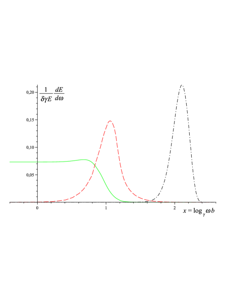
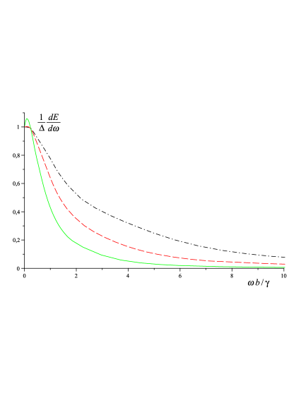
The frequency distribution in four dimensions is given in Fig. 4(b).

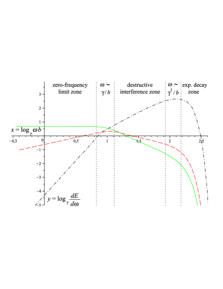
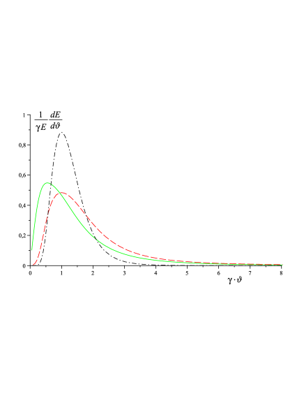
Spectral-angular characteristics. The frequency distribution curves in logarithmic $x-$scale are presented in Fig. 3: in linear scale of $dE/d\omega$ (a) and, to illustrate the rate of growth/fall, in logarithmic $y-$scale (b). Curves at the destructive-interference region $x\in(1,2)$ on the subfigure (b) represent straight lines with integer tangents $d-2$, confirming the general idea (4.2), while at low frequencies ($x<0$) any curve has an asymptote with integer tangent $d$, to confirm an idea (4.21).

Figure 3: Frequency distribution of emitted energy in linear (a), normalized by a factor $\delta=\Gamma^{4}\!\left(\frac{d+1}{2}\right)$, and logarithmic (b) $y$-scale as function of ${\rm log}_{\gamma}(\omega b)$ for $\gamma=10^{3}$. The dimensions are: $d=0$ (green, solid), $d=1$ (red, dashed) and $d=5$ (black, dot-dashed).

The angular distribution $dE/d\vartheta$ curves are presented on Fig. 4(a).

4.2 The ADD bremsstrahlung

Among the higher-dimensional scenarios the models with direct Kaluza-Klein modes, where the bulk represents compactification on a torus $T^{d}$, are of particular history and significance. Here the transformation between $D-$dimensional couplings and their four-dimensional colleagues can be established directly, via the dimensional reduction of an action.

The $D-$dimensional propagator is split on the corresponding tower of KK modes:

$$\frac{1}{q_{M}q^{M}}\to\frac{1}{V}\sum_{l\in\mathbb{Z}^{d}}\frac{1}{q_{\mu}q^{\mu}-l^{2}/R^{2}}\,\qquad\qquad\mu=0\ldots 3\,,$$

where $R$ stands for the compactification radius and $V=(2\pi R)^{d}$ is a volume of extra dimensions.

Thus, concerning our computation, the momentum integrals $I$, $I^{M}$, $J$ and $J^{M}$ introduced above, arise as a sum over integer-valued momentum inside the argument of the Macdonald functions. The summand represents (3.7) with $d=0$ and the argument of the Macdonald functions $z_{l}=\left({z^{2}+l^{2}b^{\hskip 0.70004pt2}/R^{2}}\right)^{1/2}$, both divided by a normalizing factor $V$. Thus upon the transfer from summation to integration according to the Euler – Maclaurin rule

$$\frac{1}{V}\sum_{l\in\mathbb{Z}^{d}}\hat{K}_{\lambda}\!\left(\sqrt{z^{2}+l^{2}b^{\hskip 0.70004pt2}/R^{2}}\right)\to\frac{1}{V}\int\hat{K}_{\lambda}\!\left(\sqrt{z^{2}+l^{2}\hskip 1.00006ptb^{\hskip 0.70004pt2}/R^{2}}\right)\,d^{\hskip 0.70004ptd}\hskip 0.59998ptl=\frac{1}{(2\pi)^{d/2}b^{\hskip 0.70004ptd}}\,\hat{K}_{\lambda+d/2}(z)$$ (4.14)

(for derivation see GKST2 ) in the final result one restores the expression (3.7) with ”actual” $d$.

(a)   Angular distribution $dE/d\vartheta$ of the emitted energy ($\gamma=10^{3}$) for $d=0$ (green, solid), $d=1$ (red, dashed) and $d=5$ (black, dot-dashed), normalized by the total emitted energy $E$.

(b)  Frequency distribution plots for ADD-bremsstrahlung for $d=0$ (green, solid), $d=2$ (red, dashed) and $d=5$ (black, dot-dashed) ($\gamma=10^{3}$), normalized by the ZFL factor $\Delta=\Gamma^{2}(d/2+1)/(3\cdot 2^{5}\pi^{d+4})$.

Figure 4: Angular and frequency distributions.

Apart from the features common to higher-dimensional models, the ADD scenario has some particular properties:

• the SM fields and massive particles live on the 3-brane, while gravity is essentially higher-dimensional;

• ADD is initially proposed as linearized theory of gravity.

Thus in order to evaluate electromagnetic bremsstrahlung by gravity-mediated collisions we can not apply some special cases among those derived before: indeed, $D=4$ does not allow for gravity to propagate in the bulk, while $D>4$ does allow for the vector field to live in the bulk.

Meanwhile, the linearized action for gravitational part

$$S_{g}=\int\left[-\frac{1}{4}h^{MN}\Box h_{MN}+\frac{1}{4}\,h\,\Box h-\frac{1}{2}\,h^{MN}\,h_{,MN}\,+\frac{1}{2}\,h^{MN}\,h^{P}_{N,MP}\right]d^{\hskip 0.70004ptD}x\,,$$ (4.15)

and corresponding spin-zero (spin-one) field lead to the essentially same picture after KK-summation, as initially $D$-dimensional gravity with $D-$dimensionally massless photon (graviton), as it was shown in GKST3 ; GKST4 .

In what follows we have to take a $D-$dimensional source $j^{M}$ and substitute it into the radiation formula (2.37) for $d=0$, where we vanish the bulk components $M=4\ldots D-1$. Thus the photon wave vector is parametrized by $k^{M}=(k^{\hskip 0.70004pt\mu},0,\ldots,0)$, with

$$k^{\hskip 0.70004pt\mu}=\omega\left(1,\sin\theta\cos{\varphi},\sin\theta\sin{\varphi},\cos\theta\right)\,.$$ (4.16)

Thereby, two KK propagators, corresponding to the interaction in a source, sit inside the $D-$dimensional amplitudes $j$ and $j^{*}$, while a third propagator from the Green’s function in (2.34) appears with normalization factor. Meanwhile, the model allows for the emitted photon to propagate only along the brane, that implies only zeroth emitted mode. Thus the sum degenerates into a single term while the normalizing factor survives. Eventually, the formula for the emitted energy via the electromagnetic field in ADD reads

$$E_{\rm ADD}=-\frac{1}{16\pi^{3}V}\int\limits_{0}^{\infty}\omega^{2}\,d\omega\int\limits_{S^{2}}\!\!d\Omega\,j^{*}_{\mu}(k)\,j^{\mu}(k)=\frac{1}{16\pi^{3}V}\sum_{i=1,2}\int\limits_{0}^{\infty}\omega^{2}\,d\omega\int\limits_{S^{2}}\!\!d\Omega\,\left|j_{\mu}(k)\,\varepsilon^{\mu}_{i}\vphantom{d^{0}_{0}}\right|^{2}\,.$$ (4.17)

In other words, we take the four-dimensional formula for radiation (normalized by $V$) and put a $D-$dimensional source projected on the four-dimensional sector: $\displaystyle\left.j^{\mu}(k^{\nu})=j^{M}(k)\,\delta^{M}_{\mu}\right|_{k^{i}=0}$.

Thus we use the four-dimensional coordinate system (Fig. 1, b) (with angles $\theta,\varphi$) for parametrization of the emitted photon and keep $D-$dimensional angles $\vartheta,\phi$ (Fig. 1, c) for the parametrization of interaction graviton.

The on-shell condition now reads $k_{\mu}k^{\hskip 0.70004pt\mu}=0$; taking into account, that basis vectors $u^{M}$, ${u^{\prime}}^{M}$ and $b^{\hskip 0.41998ptM}$ do not contain bulk components, it is enough to take higher-dimensional amplitudes $\rho(k)$ and $\sigma(k)$ and two polarization vectors (2.38) and (2.39)

$$\varepsilon_{1}^{\hskip 0.70004pt\mu}=\frac{1}{\gamma vz^{\prime}\sin\theta}\left[z\hskip 1.00006ptu^{\prime\mu}-z^{\prime}u^{\mu}+\left(\gamma-\frac{z}{z^{\prime}}\right)\frac{b\,k^{\mu}}{\gamma v}\right],\qquad\qquad\varepsilon_{2}^{\hskip 0.70004pt\mu}=\frac{b}{\gamma^{2}v^{2}z^{\prime}\sin\theta}\;\epsilon^{\hskip 0.41998pt\mu\nu\lambda\rho}\,u_{\nu}u^{\prime}_{\lambda}k_{\rho}\,,$$ (4.18)

where in addition, contractions (2.41) hold under appropriate substitutions $\vartheta\to\theta,\phi\to\varphi$.

To iterate, one takes $\rho(k)$ by (3.9) plus $\sigma(k)$ in the integral representation (3.2), square and integrate with measure $\omega^{2}$. Thus all notes on the destructive interference are still valid. Eventually, multiplying by $\omega^{2}$ leads to the same behavior as in four dimensions, due to the hatted Macdonald function $\hat{K}_{\nu}(x)$ goes like $\mathcal{O}\hskip 0.59998pt(1)$ at the range $x=0\ldots\mathcal{O}\hskip 0.59998pt(1)$ for any non-negative index $\nu$. So the four-dimensional behavior of the frequency distribution is reproduced, with some numerical corrections. Respectively, we repeat the strategy of computation in 4D presented above.

Thus the characteristic frequency and angle are given by

$$\omega_{\rm ADD}\sim\omega_{0}=\frac{\gamma}{b}\,,\qquad\qquad\theta\sim\bar{\vartheta}=\frac{1}{\gamma}\,,$$ (4.19)

i.e. one has beaming in forward direction with respect to the charged particle’s motion. The total emitted energy reads

$$E_{\rm ADD}=\bar{C}_{d}\,\frac{(em^{\prime}\varkappa_{D}^{2})^{2}}{b^{\hskip 0.70004pt2d+3}V}\,\gamma^{3}\,,$$ (4.20)

with coefficient $\bar{C}_{d}$ to be defined numerically. The results of numerical computation (overall coefficients $\bar{C}_{d}$) are listed here: $\bar{C}_{1}=4.90\cdot 10^{-5}$, $\bar{C}_{2}=2.54\cdot 10^{-5}$, $\bar{C}_{3}=1.77\cdot 10^{-5}$, $\bar{C}_{4}=1.52\cdot 10^{-5}$, $\bar{C}_{5}=1.55\cdot 10^{-5}$, $\bar{C}_{6}=1.85\cdot 10^{-5}$, while the frequency distribution plots are shown in Fig. 4(b).

ZFL of the frequency distribution. Given that the stress part (3.2) of the radiation amplitude is finite (for $d=0$) and vanishes for $d>0$ at the limit $\omega\to+0$, the zero-frequency limit of $dE_{\rm ADD}/d\omega$ is determined by the imaginary part of the local amplitude (3.11): indeed

$$j^{\hskip 0.41998pt\mu}(k)=-i\,\frac{\lambda\,{\rm e}^{i(kb)}}{2}\left(\frac{z^{\prime}\sin\theta\cos\varphi}{z}\,u^{\hskip 0.41998pt\mu}+\frac{b^{\hskip 0.70004pt\mu}}{b}\right)\frac{\hat{K}_{d/2+1}(z)}{z}\sim\frac{1}{\omega},$$ (4.21)

while the other terms are regular or diverge logarithmically (for $d=0$) at $\omega\to 0$. Such a behavior in $\omega$ is reminiscent of the infrared divergence of the corresponding Feynman diagrams. However, upon multiplication by $\omega^{2}$ from the measure of integration, it contributes a finite amount to the radiation loss.

Taking the finite limit of hatted Macdonald $\hat{K}_{n}(z)=2^{n-1}\Gamma(n)$ (for $n>0$) and omitting the phase factors

$$j^{\hskip 0.41998pt\mu}(k)\simeq\frac{\lambda\,\Gamma(d/2+1)}{2^{1-d/2}\omega\hskip 1.00006ptb\,\psi}\left(\frac{\sin\theta\,\cos\varphi}{\gamma\psi}\,u^{\hskip 0.41998pt\mu}+\frac{b^{\hskip 0.70004pt\mu}}{b}\right),$$ (4.22)

with $\psi\equiv 1-v\cos\theta$ now.

Squaring it and substituting into the first formula (4.17), one has

$$\left.\frac{dE_{\rm ADD}}{d\omega}\right|_{\omega=0}=\frac{(em^{\prime}\varkappa_{D}^{2})^{2}\,\Gamma^{2}(d/2+1)}{2^{8}\pi^{d+5}b^{\hskip 0.70004pt2d+2}V}\,\int d\theta\,d\varphi\;\frac{\sin\theta}{\psi^{2}}\left(1-\frac{\sin^{2}\!\theta\,\cos^{2}\!\varphi}{\gamma^{2}\psi^{2}}\right),$$ (4.23)

Consecutively integrating over $\varphi$ with help of (4.7), and over $\theta$ via (A.9), the ZFL in ADD bremsstrahlung reads

$$\left.\frac{dE_{\rm ADD}}{d\omega}\right|_{\omega=0}=\frac{\Gamma^{2}(d/2+1)}{3\cdot 2^{5}\pi^{d+4}}\,\frac{(em^{\prime}\varkappa_{D}^{2})^{2}}{b^{\hskip 0.70004pt2d+2}V}\,\gamma^{2}\,.$$ (4.24)

Notice, that this formula is still valid in four dimensions.

Going back and taking into account that destructive interference suppresses not only the radiation amplitude at frequencies $\omega>\mathcal{O}\hskip 0.59998pt(\gamma/\hskip 0.59998ptb)$ – but also the flux, one concludes that frequency

$$\omega_{\rm ADD}\sim\omega_{0}=\frac{\gamma}{b}$$

gives the effective cut-off for all cases of ADD, as well as to four-dimensional bremsstrahlung. Thereby the realistic estimate is

$$E_{\rm ADD}\sim\left.\frac{dE_{\rm ADD}}{d\omega}\right|_{\omega=0}\!\!\times\omega_{\rm ADD}=\frac{\Gamma^{2}(d/2+1)}{3\cdot 2^{\hskip 0.41998pt5}\pi^{d+4}}\,\frac{(em^{\prime}\varkappa_{D}^{2})^{2}}{b^{\hskip 0.70004pt2d+3}V}\,\gamma^{3}\,.$$ (4.25)

Such an approach is used by Smarr Smarr to estimate four-dimensional gravitational bremsstrahlung.

Therefore, the vector bremsstrahlung in ADD case repeats the four-dimensional picture, up to numeric coefficient.

4.3 The UED bremsstrahlung and average number of Kaluza-Klein modes

Through the entire text we implied that (1.2) is satisfied and one has large number of KK-modes, that allows to pass from KK-summation to the continuous integration and that eventually leads to the enhancement of $\gamma-$factor power.

Meanwhile, for the UED models, where the vector field can propagate through the bulk, the contemporary constraints UED on the size of the extra dimensions, coming from the experimental data (including the recent ATLAS and CMS experiments), give the following bound:

$$1/R_{\rm UED}\sim 300-3000\,{\rm GeV}\,,\qquad\qquad R_{\rm UED}\sim 10^{-16}\,\mathrm{cm}\,.$$ (4.26)

In this case the inequality $b<R$ (1.2), combined with $b>r_{\rm cl}$, to have a charge point-like, does not hold. Does it imply that the whole derivation presented above, fails?

Consider the situation more thoroughly: we first restore the original KK-summations, before switching to integration. The analogue of (2.37) reads:

$$E=\frac{1}{16\pi^{3}V}\sum_{i}\sum_{n\in\mathbb{Z}^{d}}\int\limits_{0}^{\infty}\!\!\varpi^{2}\,d\varpi\int\limits_{S^{2}}\!\!d\Omega\,\left|j_{i}(k)\right|^{2}\left.\vphantom{\sqrt{d}}\right|_{k^{0}=\sqrt{\varpi^{2}+n^{2}b^{2}/R^{2}}}\,\qquad\qquad\varpi^{2}=\sum_{a=1}^{3}(k^{a})^{2},$$ (4.27)

with $\varpi=|\mathbf{k}|$ being a continuous frequency in four-dimensional sector.

The local current is given by (3.5), after the corresponding change of the integrals $I$ and $I^{M}$ in (3.6), given in GKST3 , to:

$$I=-\frac{2\pi}{\gamma vV}\,\sum_{l\in\mathbb{Z}^{d}}{{K}}_{0}(z_{l})\,,\qquad\qquad I^{M}=-\frac{2\pi}{\gamma v\hskip 1.00006ptb^{\hskip 0.70004pt2}V}\sum_{l\in\mathbb{Z}^{d}}\left(b\hskip 1.00006ptz\hskip 1.00006pt{{K}}_{0}(z_{l})\,\frac{\gamma u^{\prime M}-u^{M}}{\gamma v}+i\hat{K}_{1}(z_{l})\,b^{\hskip 0.41998ptM}\right),$$ (4.28)

respectively, with $z_{l}^{2}\equiv z^{2}+l^{2}b^{\hskip 0.70004pt2}/R^{2}$. A similar summation arises in the stress integrals.

When $b\gg R$, one passes in (4.28) to integration according to (4.14), and the expressions (3.7) are restored. The stress amplitude is split into the KK-sum in a similar way, for more information see GKST3 .

Such a summation appears inside the amplitude $j^{M}(k)$ and corresponds to the KK-compactification of the interaction graviton. So the effective number of KK-modes of interaction is determined by the exponential decay of Macdonald function ($l^{2}b^{\hskip 0.70004pt2}/R^{2}\lesssim 1$) and reads

$$N_{\rm int}\equiv l_{\max}=[L/\hskip 0.59998ptb]+1\,,$$ (4.29)

independent of the value $0\leqslant z\lesssim 1$.

In the ADD-case the bound on the compactification radius is $R_{\rm ADD}\sim 10^{-2}\,{\rm cm}$ (for $d=2$), and (1.2) is well satisfied, thus one has a large number of the interaction KK-modes.

In the case of UED, one has $R_{\rm UED}<l_{C}$ and one has to revisit the computation. The above condition implies that the interaction has only zeroth KK-mode.

Thus the sum in (4.28) degenerates into

$$I=-\frac{2\pi}{\gamma vV}\,K_{0}(z)\,,\qquad\qquad I^{M}=-\frac{2\pi}{\gamma v\hskip 1.00006ptb^{\hskip 0.70004pt2}V}\left(b\hskip 1.00006ptz\hskip 1.00006ptK_{0}(z)\,\frac{\gamma u^{\prime M}-u^{M}}{\gamma v}+i\hat{K}_{1}(z)\,b^{\hskip 0.41998ptM}\right),$$ (4.30)

plus exponentially-suppressed terms, and the radiation amplitude represents the expressions derived in Section 3 for $d=0$, but normalized by the factor $V$.

Therefore, the emission modes are determined by the exponential decay of Macdonalds $K_{0}(z)$ and $K_{1}(z)$. In the original KK-treatment the argument $z$ becomes dependent upon the number $n$ of emission KK-quantum as

$$z\equiv\frac{(ku)b}{\gamma v}\simeq\sqrt{\varpi^{2}b^{2}+n^{2}b^{2}/R^{2}}-\varpi b\hskip 1.00006ptv\cos\theta$$ (4.31)

In the total absence of emission KK-modes, the characteristic frequency is given by its $d=0-$value $\varpi\sim\omega_{0}$ (4.19), thus the typical value of $\varpi b$ is at least $\varpi b\gtrsim\gamma$. Assume that

$$b<R\gamma\,,$$ (4.32)

that is reasonable for $R$ given by (4.26) and $\gamma\sim 10^{14}$. Then the first massive KK-mode is available, and some number $n<N_{\rm emit}$ of first KK-modes satisfy $nb/R<\gamma$. In this case one expands the radical in (4.31) to obtain

$$z\approx\varpi b+\frac{n^{2}b}{2\hskip 1.00006pt\varpi R^{2}}-\varpi b\hskip 1.00006ptv\cos\theta=\varpi b\psi+\frac{n^{2}b}{2\hskip 1.00006pt\varpi R^{2}}$$ (4.33)

Thus the effective number of emission KK-modes

$$N_{\rm emit}\equiv n_{\max}(\varpi)=\sqrt{\frac{2\varpi R^{2}}{b}}\,,$$ (4.34)

becomes dependent on the frequency. In the most favorable case the maximal frequency is determined from the first term of the RHS of (4.33), which should be less than unity independently GKST2 : $\varpi\sim\psi^{-1}\!/\hskip 0.59998ptb\sim\gamma^{2}\!/\hskip 0.59998ptb$. Thus

$$N_{\rm emit}\sim\frac{\gamma R}{b}>1\,,$$ (4.35)

according to the necessary condition (4.32).

In addition, now assume the stronger condition :

$$\frac{\gamma R}{b}\gg 1\,,$$ (4.36)

Then $N_{\rm emit}\gg 1$, so the modes are quasi-continuous, and we combine quasi-continuous momenta with continuous $\varpi$ into single $\omega$, shift angles $(\theta,\varphi)\to(\vartheta,\phi)$ and we return to the case (4.1), where we integrate the square of radiation amplitude with volume measure

$$\mathcal{V}_{d}=\frac{1}{2(2\pi)^{d+3}}\>\omega^{d+2}\,\sin^{d+1}\!\vartheta\>d\omega\,d\vartheta\,d\Omega_{d+1}\,.$$ (4.37)

Given that the hatted Macdonald function $\hat{K}_{\nu}(z)$ alters slowly with the change of index $\nu\geqslant 0$, the integration should be performed along the same lines as in Subsection 4.1. Namely, for $d\geqslant 2$ the high-frequency regime dominates, and for the radiation amplitudes one has instead (3.4) and (3.10), the following one:

$$j_{\pm}(k)\approx\frac{\lambda_{0}\,{\rm e}^{i(kb)}\sin\vartheta}{2\sqrt{2}} \left[\frac{d+1}{d+2}\,\frac{1-\gamma^{2}\psi}{\gamma^{2}\psi}\,{K}_{0}(z)-\frac{1}{z^{2}}\left(\frac{\sin^{2}\!\vartheta}{\psi}-1\right)\hat{K}_{1}(z)+\right.$$

$$\;\;\left.+\frac{\sin^{2}\!\phi}{z^{2}}\left(\frac{\sin^{2}\!\vartheta}{\psi}-1\right)\hat{K}_{2}(z)\pm i\,\frac{\sin 2\phi}{2\,z^{2}}\,\hat{K}_{2}(z)\right],$$ (4.38)

with $\lambda_{0}\equiv e\hskip 1.00006ptm^{\prime}\hskip 0.59998pt\varkappa_{D}^{2}/2\pi V$.

Again, we split the integrals on frequency and angular parts, as in (4.4):

$$\frac{dE}{d\Omega}=\frac{\lambda_{0}^{2}\sin^{d+3}\!\vartheta}{8\left(2\pi\right)^{d+3}b^{\hskip 0.70004ptd+3}\psi^{d+3}}\sum_{a,b=0}^{2}\tilde{C}_{ab}^{(d\hskip 0.41998pt)}\tilde{D}_{ab}^{(d\hskip 0.41998pt)}(\vartheta,\phi)\,,$$ (4.39)

where $\tilde{C}_{ab}^{(d\hskip 0.41998pt)}\equiv\int\hat{K}_{a}(z)\hat{K}_{b}(z)\,z^{d+2\left(\delta_{0a}+\delta_{0b}-1\right)}\,dz\hskip 1.00006pt$. As before, these integrals are to be computed with help of (4.5).

Comparing (4.3) with (3.4), one concludes that the angular coefficient functions $\tilde{D}_{ab}^{(d\hskip 0.41998pt)}$ have the corresponding changes with respect to those ones $D_{ab}^{(d\hskip 0.41998pt)}$ given in (4.1):

$$\tilde{D}_{01}^{(d\hskip 0.41998pt)}=\frac{{D}_{01}^{(d\hskip 0.41998pt)}}{d+1}\,,\qquad\qquad\tilde{D}_{11}^{(d\hskip 0.41998pt)}=\frac{{D}_{11}^{(d\hskip 0.41998pt)}}{(d+1)^{2}}\,,\qquad\qquad\tilde{D}_{12}^{(d\hskip 0.41998pt)}=\frac{{D}_{12}^{(d\hskip 0.41998pt)}}{d+1}\,.$$

The same relations exist for the integrated over all angles constants. Combining them all and substituting to (4.39), one obtains the energy loss

$$E_{\rm UED}\approx\tilde{C}_{d}\frac{\left(em^{\prime}\varkappa_{D}^{2}\right)^{2}}{V^{2}b^{\hskip 0.70004ptd+3}}\>\gamma^{d+2}\,.$$ (4.40)

The values of $\tilde{C}_{d}$ for small values of the number of extra dimensions are listed as: $\tilde{C}_{2}=7.8\cdot 10^{-6}$, $\tilde{C}_{3}=1.5\cdot 10^{-6}$, $\tilde{C}_{4}=4.5\cdot 10^{-7}$, $\tilde{C}_{5}=1.7\cdot 10^{-7}$.

$\boldsymbol{d=1.}$ Repeating the same arguments, we compute the total radiation numerically:

$$E=\tilde{C}_{1}\frac{\left(em^{\prime}\varkappa_{5}^{2}\right)^{2}}{V^{2}b^{\hskip 0.70004pt4}}\>\gamma^{3}\hskip 1.00006pt\ln\gamma\,,\qquad\qquad\tilde{C}_{1}=2.82\cdot 10^{-5}\,.$$ (4.41)

The spectral characteristics in UED bremsstrahlung are the same as in higher-dimensional case (Subsection 4.1), while the angular characteristics are similar to all cases considered above.

A summary. In Table II we summarize the ultimate cases of an ultrarelativistic bremsstrahlung from the viewpoint of average numbers of the Kaluza-Klein modes excited in the bremsstrahlung process.

		hhhh $N_{\rm int}\lesssim 1$	hhh $N_{\rm int}\gg 1$
$N_{\rm emit}\lesssim 1$	$\begin{array}[]{rc}\rule{0.0pt}{13.00005pt}\text{\footnotesize space-time model}=&\\ \text{\footnotesize characteristic frequency}=&\\ \text{\footnotesize radiation amplitude}=\\ \text{\footnotesize phase volume}=\\ \text{\footnotesize KK modes}=\\ \text{\footnotesize emitted energy}=\end{array}$	$\begin{array}[]{l}\rule{0.0pt}{13.00005pt}M_{1,3}\\ \omega\sim\omega_{\hskip 0.41998pt0}\\ j=j_{\hskip 0.41998pt0}\\ \mathcal{V}=\mathcal{V}_{0}\\ N_{\rm int}=N_{\rm emit}=1\\ \gamma^{3}\end{array}$	hi $\begin{array}[]{l}\rule{0.0pt}{13.00005pt}\text{ADD}\\ \omega\sim\omega_{\hskip 0.41998pt0}\\ j=j_{\hskip 0.41998ptd}\\ \mathcal{V}=\mathcal{V}_{0}/V\\ N_{\rm emit}=1\\ \gamma^{3}/V\end{array}$
$N_{\rm emit}\gg 1$	$\begin{array}[]{rc}\rule{0.0pt}{13.00005pt}\text{\footnotesize space-time model}=&\\ \text{\footnotesize characteristic frequency}=&\\ \text{\footnotesize radiation amplitude}=\\ \text{\footnotesize phase volume}=\\ \text{\footnotesize KK modes}=\\ \text{\footnotesize emitted energy}=\end{array}$	$\phantom{h,}\begin{array}[]{l}\rule{0.0pt}{13.00005pt}\text{UED}\\ \omega\sim\gamma\omega_{\hskip 0.41998pt0}\\ j=j_{\hskip 0.41998pt0}/V\\ \mathcal{V}=\mathcal{V}_{d}\\ N_{\rm int}=1\\ \gamma^{d+2}\!/V^{2}\end{array}$	hi $\begin{array}[]{l}\rule{0.0pt}{13.00005pt}M_{1,d+3}\\ \omega\sim\gamma\omega_{\hskip 0.41998pt0}\\ j=j_{\hskip 0.41998ptd}\\ \mathcal{V}=\mathcal{V}_{d}\\ N_{\rm emit}=\gamma N_{\rm int}\\ \gamma^{d+2}\end{array}$

Table 2: The qualitative relation between the cases of gravity-mediated vector bremsstrahlung from viewpoint of number of KK-modes. The values are normalized as $\lambda=b=e=1$. $N=1$ implies that only the zeroth KK-mode is actual. The measure of the phase volume integration is defined by (4.37).

5 Discussion

According to the computation presented above, we overview possible effects and give the estimates on them.

5.1 Scattering of two charges

When both particles are charged by the vector field $A^{M}$ then the direct electromagnetic interaction is expected to be the dominant force. Then the acceleration (and, being integrated, the trajectory deflection) represents (to first order of PT) the sum of two contributions of electromagnetic and gravitational nature, respectively. In turn, these addenda to trajectory may lead to radiation via vector and tensor fields. We do not consider gravitational waves in this work, and thus focus here to the pure vector bremsstrahlung.

A similar approach (i.e. bremsstrahlung without accounting for gravity) was considered in GKST2 for the scalar bremsstrahlung, so it is not necessary to reproduce that computation in details. Instead of the detailed computation, we highlight the main steps and overview the results.

Making use of perturbation theory over $e$ and considering (2.2) on the flat background with $F_{MN}$ (3.1) generated by charge $e^{\prime}$, the acceleration on trajectory reads:

$$\,^{1}\!\hskip 1.00006pt\ddot{z}^{M}_{\rm em}(\tau)=i\,\frac{e^{\prime}e}{(2\pi)^{d+3}m}\int d^{\hskip 0.70004ptD}q\frac{\delta(qu^{\prime})}{q^{2}}\;e^{-iqb}e^{-i(qu)\tau}\left[\vphantom{\frac{a}{a}}\gamma\hskip 1.00006ptq^{M}-(qu)\,u^{\prime M}\right].$$ (5.1)

The scattering angle, computed along the same lines as in GKST1 , is given by

$$\alpha_{\rm em}\sim\frac{e\,e^{\prime}}{m\,\gamma\,b^{\hskip 0.70004ptd+1}}\sim\left[\frac{\sqrt{r_{\rm cl}r^{\prime}_{\rm cl}}}{b}\,\frac{\sqrt{m^{\prime}}}{\sqrt{m}}\right]^{d+1}\frac{1}{\gamma}<\frac{(m^{\prime}/m)^{\frac{d+1}{2}}}{\gamma}\,.$$ (5.2)

Performing the perturbation-theory scheme (with the obvious restriction $b>r_{\rm cl}$), one obtains the following second-order source valid in all frequency regimes:

$$j^{M}(k)\sim i\,{\rm e}^{i(kb)}\,\frac{e^{2}\,e^{\prime}}{m\gamma b^{\hskip 0.70004ptd}}\,\left(\frac{\sin\vartheta\cos\phi}{\gamma\psi}\,u^{M}+\frac{b^{\hskip 0.41998ptM}}{b}\right)\frac{\hat{K}_{d/2+1}(z)}{z}\,.$$ (5.3)

It is produced by the fast particle, while the corresponding terms due to the target and the interference give subleading in $\gamma$ contribution.

As was mentioned above, such an argument of the Macdonald function leads to the dominance of $z-$region in the entire spectrum. Thus in the Lab frame the characteristic spectral-angular values are:

$$\omega_{\rm em}\sim\frac{\gamma^{2}}{b}\,,\qquad\qquad\vartheta_{\rm em}\sim\frac{1}{\gamma}\,,$$ (5.4)

On the other hand we see that such a behavior at low frequencies leads to the finite ZFL of frequency distribution, which for the case of non-compactified extra dimensions reads

$$\left(\frac{1}{\omega^{d}}\frac{dE}{d\omega}\right)_{\!\omega=0}\sim\frac{(e^{2}\,e^{\prime})^{2}}{b^{\hskip 0.70004pt2d+2}}\,\gamma^{-d}\,.$$ (5.5)

Here no process which drastically changes the amplitude (like destructive interference) occurs in the whole frequency domain $\omega\in[0,\omega_{\rm em}]$, and one applies ZFL-approximation with maximal frequency given by (5.4):

$$E_{\rm em}\sim\left(\frac{1}{\omega^{d}}\frac{dE}{d\omega}\right)_{\!\omega=0}\!\!\times\omega_{\rm em}^{d+1}\sim\frac{e^{4}\,{e^{\prime}}^{2}}{m^{2}b^{\hskip 0.70004pt3(d+1)}}\,\gamma^{d+2}\,.$$ (5.6)

Roughly speaking, the total emitted energy carried by the vector field is twice that of the scalar situation due to the two polarization states, after making the identifications $f\to e,f^{\hskip 0.70004pt\prime}\to e^{\prime}$, respectively. Therefore most of emitted waves are beamed into the cone with characteristic angle $1/\gamma$.

The efficiency is given by

$$\epsilon_{\rm em}\sim\left(\gamma\,\frac{r_{\rm cl}^{3}}{b^{\hskip 0.70004pt3}}\right)^{\!\!1+d}.$$ (5.7)

Taking into account that when interacting gravitationally, the charge emits $E_{\mathrm{rad}}\sim\gamma^{3}$ in four dimensions, while only $E_{\rm em}\sim\gamma^{2}$ in Coulomb-field collision, it seems intriguing to derive that value of $\gamma$, for which the two contributions become comparable.

Correction to gravity-mediated vector bremsstrahlung. The acceleration of both particles in the first order of PT represents the sum of gravitational and Lorentz-force parts. The electromagnetic part causes $e^{2}\,e^{\prime}-$contribution to the vector current and leads to the pure electromagnetic bremsstrahlung reviewed above in this Subsection.

The appearance of a second charge $e^{\prime}$ (with mass $m^{\prime}$) adds some terms to the radiation amplitudes: namely, local (3.11) and non-local (3.2) parts will acquire addenda $\rho^{\prime}(k)$ and $\sigma^{\prime}(k)$, based on the integrals (3.6) and (3.13) where primed and unprimed quantities are mutually interchanged. These terms also can be derived in the same way in the Lorentz frame associated with $e-$charge (comoving frame), and then Lorentz-transformed into the Lab frame. With $e$ and $e^{\prime}$ to be of the same order, in the comoving frame the emission is dominant due to these new terms, and governed by Macdonald function $K_{\nu}(z^{\prime})$. Hence in this frame the emission is beamed inside the cone $\vartheta^{\hskip 0.41998pt\prime}\lesssim 1/\gamma$ with respect to $\mathbf{u}^{\prime}$. Being transformed to the Lab frame, these terms remain to be $K_{\nu}(z^{\prime})$ since $z^{\prime}$ is a Lorentz-scalar (3.8). Thus these addenda are not important in higher frequencies and represent subleading, by an order of $\gamma$ terms (with respect to the terms we keep) due to the Lorentz transformation, with a corresponding interchange of primed and unprimed couplings in (4.11).

The conservation of these terms is easily verified using the same strategy as for the basic terms. The self-action terms appearing here, are discussed in Appendix  B.

5.2 Coherence length

In this subsection we consider qualitatively the effects arising in the bremsstrahlung process, and the spectrum of emitted waves, from the viewpoint of coherence length, coming from consideration of the particle’s equation of motion in the presence of external field.

While accelerating, the particle emits radiation. Its spectral characteristics are translated from the corresponding temporal ones, related with the duration of accelerated motion, and with the value of acceleration and type of external force.

Apart from the formulae for the total energy loss on radiation in the coordinate and momentum representations given in subsection 2.3, the intensity of electromagnetic emission can be characterized by the square of the incomplete Fourier-transform of $A^{M}(x)$ considered as an integral over the particle’s classical trajectory $z^{M}(\tau)$:

$$A^{M}(\omega,\mathbf{r})\sim\frac{e}{\rho}\int u^{M}(\tau)\,{\rm e}^{i(\omega t-\mathbf{k}\mathbf{z})}\,d\tau\,,\qquad\qquad\rho\equiv|\mathbf{r}-\mathbf{z}|\,.$$

Being squared, the combination $|A^{M}(\omega,\mathbf{r})|^{2}$ contains a double integral over $\tau_{1}\tau_{2}$ with ${\rm e}^{ik\hskip 0.70004pt\cdot\Delta z}$ in the integrand.

Expanding $\Delta z^{M}=u^{M}+\ddot{z}^{M}\tau+\dddot{z}^{M}\tau^{2}/2+\ldots$, where $\tau\equiv\tau_{2}-\tau_{1}$, the difference in the phases of the two waves emitted by a charge in the same direction $\mathbf{n}$ at close moments $\tau_{1}$ and $\tau_{2}$ of proper time, is determined by

$$\Delta\varphi=k\cdot\Delta z=\omega\left[\rule{0.0pt}{10.00002pt}t-\mathbf{n}\,\Delta\mathbf{z}(t)\right]\,,\qquad\qquad t\equiv\tau_{2}-\tau_{1}\,.$$

In addition, in ultrarelativistic motion the transverse component of the force acts much more effectively than the longitudinal one. Because of this, one can transit from $D-$dimensional expansions to their spatial sector, and the latter equation can be rewritten as

$$\Delta\varphi=\omega t\left(1-\mathbf{n}\mathbf{v}-\frac{t}{2}\,\mathbf{n}\mathbf{\dot{v}}+\frac{t^{2}}{6}\,\mathbf{\dot{v}}^{2}+\ldots\right)$$

Thus to the leading order $\Delta\varphi\approx\omega t\hskip 0.59998pt(1-\mathbf{n}\mathbf{v})=\omega t\hskip 0.59998pt(1-v\cos\vartheta)=\omega t\hskip 0.59998pt\psi\,.$ When $\Delta\varphi$ becomes of order $\mathcal{O}\hskip 0.59998pt(1)$, the waves with antiphase are present in the spectrum, so they annihilate and decoherence happens.

Thus the maximal duration of coherence is given by

$$t_{\rm coh}\sim\frac{1}{\omega\hskip 0.59998pt\psi}\,,\qquad\qquad\tau_{\rm coh}\sim\frac{t_{\rm coh}}{\gamma}\sim\frac{1}{\omega\hskip 0.59998pt\gamma\hskip 0.59998pt\psi}\,.$$ (5.8)

Let us consider the wave formed within the coherence length (during the coherence time) and emitted in the angle $\vartheta$ with respect to $\mathbf{u}$. The characteristic duration of this signal in the Lab frame is determined by the difference of distances covered by two waves, emitted at the start and finish of the coherence interval and received far from the particle’s location. Computing it, one obtains $t_{\hskip 0.41998pt\rm Lab}=(1-v\cos\vartheta)\,t_{\rm coh}=\psi\hskip 1.00006ptt_{\rm coh}$. Going back to all cases of bremsstrahlung, most of the emitted radiation is beamed inside the cone $\vartheta\lesssim\bar{\vartheta}=1/\gamma$, that is confirmed by the curves in Fig. 4(a).

Given that at coherence interval the deflection angle should be $\alpha<\gamma^{-1}$, the Lab-frame duration is estimated as

$$t_{\rm Lab}\simeq\frac{\vartheta^{2}+\gamma^{-2}}{2}\>t_{\rm coh}\,.$$ (5.9)

Finally, using (5.8) one has:

$$\omega_{\rm com}\sim\frac{1}{t_{\rm coh}}\,,\qquad\qquad\omega\sim\frac{1}{t_{\rm coh}\psi}\sim\frac{1}{t_{\rm Lab}}\sim\gamma^{2}\omega_{\rm com}\,.$$ (5.10)

The frequency in the Lab frame is, thereby, $\gamma^{2}$ larger than the frequency in the comoving frame, according to the Doppler effect.

Therefore we analyze the average time of accelerated motion.

Classical electrodynamics. Expanding (5.1) near $\tau=0$ one deduces that the acceleration is determined by the transverse component $\,{}^{1}\!\hskip 1.00006pt\ddot{z}^{\hskip 0.70004ptx}_{\rm em}$ with characteristic value

$$\,^{1}\!\hskip 1.00006pt\ddot{z}^{\hskip 0.70004ptx}_{\rm em}(0)\sim\frac{ee^{\prime}}{m}\,\frac{\gamma}{b^{\hskip 0.70004ptd+2}}\,.$$ (5.11)

The duration of the accelerated motion is characterized by that interval, for which the trajectory is deflected on an angle, comparable to the total deflection angle $\alpha_{\rm em}$ given by (5.2):

$$\tau_{\rm em}\sim\frac{b}{\gamma}\,,\qquad\qquad t_{\rm em}\sim b\,.$$ (5.12)

For details, see Spir . Next, consider the radiative part of the Lorentz-Dirac force in higher dimensions: it is determined by averaging over angles of the corresponding part of energy-momentum tensor, the latter reads $T_{\rm em}^{\rm emit}\sim e^{2}/r^{d+2}$, where $r$ stands for the retarded Lorentz-invariant distance parameter (for construction see Spir-2009 ).

For instance, in four dimensions it represents well-known (relativistic) Larmor formula for the emission intensity (in the units we use)

$$\frac{d{E}_{\rm rad}}{dt}=-\frac{1}{6\pi}\,e^{2}\ddot{z}^{\hskip 0.70004pt2}_{\rm em}\,,\qquad\qquad\dot{E}_{\rm rad}=-\frac{1}{6\pi}\,e^{2}\ddot{z}^{\hskip 0.70004pt2}_{\rm em}\dot{z}^{0}\,.$$

In even higher dimensions the analogue of the Larmor formula can be computed in the a closed form and reads schematically (in the gauge $\dot{z}^{2}=1$)

$$\dot{E}_{\rm rad}\sim e^{2}\gamma\left[B_{\scriptstyle\underbrace{\scriptstyle(2,2;\hskip 0.41998pt2\ldots 2)}_{d+2}}\;(\ddot{z}_{\rm em}^{\hskip 0.70004pt2})^{\hskip 0.41998ptd/2+1}+\ldots+B_{(D/2,D/2)}\left(z_{\rm em}^{(D/2)}\cdot z_{\rm em}^{(D/2)}\right)\right]\,.$$ (5.13)

with some positively defined form in the parenthesis. Here $B_{(\alpha_{k\ldots})}$ is a constant with list of orders of derivatives, constituting the corresponding scalar products, while dots represent all intermediate scalar terms with the same dimensionality of mass ($[m]={\rm cm}^{-1}$).

Taking into account that for higher derivatives

$$\frac{d^{D/2}}{d\tau^{D/2}}\,\,^{1}\!\hskip 1.00006ptz^{M}_{\rm em}\sim\,^{1}\!{z^{x}_{\rm em}}^{(D/2)}\sim\,^{1}\!\hskip 1.00006pt{\ddot{z}^{x}_{\rm em}}\,\frac{\gamma^{d/2}}{b^{\hskip 0.70004ptd/2}}\,,$$

that follows from (5.1), and substituting (5.11), one obtains the estimate

$$\,^{1}\!\hskip 1.00006pt{z^{x}_{\rm em}}^{(D/2)}\sim\frac{e\hskip 0.59998pte^{\prime}}{m}\,\frac{\gamma^{d/2+1}}{b^{\hskip 0.70004pt3d/2+2}}\,.$$ (5.14)

Given that all terms in the parenthesis have the same total dimensionality ${\rm cm}^{-(d+2)}$, and that each derivative adds $\gamma/\hskip 0.59998ptb$, one concludes that all terms have the same order of $\gamma-$factor. In what follows, the leading term is determined by the perturbation theory, and given by the term with minimal number of scalar products, namely, the last term in (5.13). From the dimensional analysis it is easy to see that all other terms contain more than two first-order kinematical quantities.

Thus the total emitted energy during the whole bremsstrahlung process is given by

$$E_{\rm em}\sim e^{2}\left[\,{}^{1}\!\hskip 1.00006pt{z^{x}_{\rm em}}^{(D/2)}\right]^{2}t_{\rm em}\sim\frac{e^{4}{e^{\prime}}^{2}}{m^{2}}\,\frac{\gamma^{d+2}}{b^{\hskip 0.70004pt3d+3}}\,,$$ (5.15)

in agreement with (5.6). Thus the estimate of vector bremsstrahlung as induced emission of a charge in the external Coulomb field is valid within the same perturbation theory.

Finally, (5.12) represents the coherence length of emitted waves in the comoving Lorentz frame – the characteristic length of the trajectory, where the signal is formed. Applying the transformation (5.10)) to (5.12, one obtains

$$\omega_{\rm em}\sim\frac{1}{t_{\rm em}\psi}\sim\frac{\gamma^{2}}{b}$$ (5.16)

in the Lab frame, in agreement with (5.4).

Classical electrodynamics in external curved background. The deflection angle in a static gravitational potential in $D$ dimensions is given by GKST1

$$\alpha_{\rm gr}\sim\frac{{r^{\prime}_{g}}^{d+1}}{b^{\hskip 0.70004ptd+1}}\ll 1\,,$$ (5.17)

and, according to the Equivalence principle, does not depend upon the energy of the scattered particle.

Double-differentiating (3.4), one obtains the estimate of the transverse component of an acceleration caused by the gravitational force:

$$\,^{1}\!\hskip 1.00006pt\ddot{z}_{\rm gr}^{x}(0)\sim\frac{{r^{\prime}_{g}}^{d+1}\gamma^{2}}{b^{\hskip 0.70004ptd+2}}\,,$$ (5.18)

while the characteristic time of acceleration is governed, essentially, by the same factors as before and reads

$$\tau_{\rm gr}\sim\frac{b}{\gamma}\,,\qquad\qquad t_{\rm gr}\sim b\,.$$ (5.19)

Nevertheless, the dominant contribution into $\ddot{z}^{\hskip 0.70004pt2}(\tau)$ is given by domains $\tau\sim b/\gamma$ and $\tau\sim-b/\gamma$ where $|\,^{1}\!\hskip 1.00006pt\ddot{z}_{\rm gr}^{\hskip 0.41998pt0}|$ reaches its maximum, despite the fact that at $\tau=0$ it vanishes:

$$\,^{1}\!\hskip 1.00006pt\ddot{z}_{\rm gr}^{\hskip 0.41998pt0}(\pm\tau_{\rm gr})\sim\frac{{r^{\prime}_{g}}^{d+1}}{b^{\hskip 0.70004ptd+2}}\,\gamma^{2}\,,\qquad\qquad\,^{1}\!\hskip 1.00006pt\dot{z}_{\rm gr}^{\hskip 0.41998pt0}(\pm\tau_{\rm gr})\sim\frac{{r^{\prime}_{g}}^{d+1}}{b^{\hskip 0.70004ptd+1}}\,\gamma\,\,{}^{*}.$$ (5.20)

If the space-time the had been flat, the direct application of estimate (5.15) would lead to the result

$$E_{\rm em/curve}\sim e^{2}\left[\,{}^{1}\!\hskip 1.00006pt{z^{x}_{\rm gr}}^{(D/2)}\right]^{2}t_{\rm gr}\sim e^{2}G_{D}^{2}{m^{\prime}}^{2}\,\frac{\gamma^{d+4}}{b^{\hskip 0.70004pt3d+3}}\,.$$ (5.21)

However, not only is this result overestimated – it totally vanishes due to the following reasoning.

The analogue of Larmor formula in four dimensions in a fixed curved space-time is given by the finite part of formula by de Witt and Brehme DeWitt:1960fc , corrected by Hobbs Hobbs :

$$f^{\hskip 0.70004pt0}_{\rm em}(\tau)=\frac{e^{2}}{4\pi}\left[\Pi^{0\nu}\!\!\left(\frac{2}{3}\,D^{2}\dot{z}_{\nu}+\frac{1}{3}\,R_{\nu\lambda}\hskip 1.00006pt\dot{z}^{\lambda}\right)+\dot{z}^{\nu}(\tau)\!\!\int\limits_{-\infty}^{\tau}\!\!\!\left(\vphantom{\frac{a}{a}}v^{\hskip 0.41998pt0}{}_{\lambda^{\prime};\nu}-v_{\nu\lambda^{\prime}}{}^{;0}\right)\dot{z}^{\lambda^{\prime}}(\tau^{\prime})\,d\tau^{\prime}\right],\qquad\qquad\Pi^{\hskip 0.70004pt\mu\nu}\equiv g^{\hskip 0.70004pt\mu\nu}-\frac{\dot{z}^{\mu}\dot{z}^{\nu}}{\dot{z}^{2}}\,,$$ (5.22)

Here $v^{\nu\alpha}$ represents the non-local part of the vectorial Green’s function in a curved background in terms of bi-tensor quantities, evaluated at points $z^{\mu}(\tau)$ and $z^{\mu^{\prime}}(\tau^{\prime})$.

In flat background one has $g_{\mu\nu}\to\eta_{MN}\delta^{M}_{\mu}\delta^{N}_{\nu}$, $D\dot{z}^{\mu}\to\ddot{z}^{M}\delta_{M}^{\hskip 0.70004pt\mu}$, $D^{2}\dot{z}^{\mu}\to\dddot{z}^{M}\delta_{M}^{\hskip 0.70004pt\mu}$ etc., and (5.22) passes into the Lorentz-Dirac equation, there the radiative part is constituted from the radiation part $\sim\ddot{z}^{2}\,\dot{z}^{M}$ and radiation-reaction (”Schott”) part $\sim\dddot{z}^{M}$.

The ”Larmor” part here is given by

$$\frac{1}{6\pi}\,e^{2}\,\Pi^{0\nu}\,D^{2}\dot{z}_{\nu}=\frac{1}{6\pi}\,e^{2}\left[D\dot{z}_{\nu}D\dot{z}^{\nu}\,\dot{z}^{0}+D^{2}\dot{z}^{0}\vphantom{\frac{a}{a}}\right]\,.$$ (5.23)

But the charge is moving across the geodesics, hence the covariant acceleration $D\dot{z}^{\hskip 0.70004pt\mu}$ and its covariant derivatives vanish. The local term with Ricci-tensor of the exact metric also vanishes outside the source. Thus in the total-metric description all radiation effects come from the tail term in (5.22). The same structure of tail term appears in any dimensionality.

Instead of derivation of tail integral according to the total metric, we consider the perturbation theory and give a direct correspondence to reconcile with what we do. In fact, we have been computing the lower orders of constituents of equation (5.22).

In this case one can expect deflections from the common rule.

First we check that $D\dot{z}^{M}$ is still zero in the first order: indeed, as it follows from (2.3), the flat derivative $\,{}^{1}\!\ddot{z}^{M}$ is given by double derivative of (3.4), while the Christoffel part is given by (2.2) and (3.1). Roughly speaking, their sum is (3.28,b) contracted with ${u^{\prime}}^{N}$ and thus vanishes. The next orders do not affect on the order $(r^{\prime}_{g}/\hskip 0.59998ptb)^{2}$ we need. The same concerns the covariant derivatives of covariant acceleration in higher dimensions.

Now consider the Ricci-term. In the first order of PT the Newton field coincides with the linearized Schwarzschild metric and thus still represents Ricci-flat space-time outside the $m^{\prime}$:

$$R_{\lambda\rho}\!\left[\eta_{\mu\nu}+\varkappa_{D}\,^{1}\!h_{\mu\nu}^{\rm[PL]}\right]=\mathcal{O}\hskip 0.59998pt\!\left({(r^{\prime}_{g}/r)^{2}}\right)\,,\qquad\qquad R_{\lambda\rho}\!\left[\eta_{\mu\nu}+\varkappa_{D}\,^{1}\!h_{\mu\nu}^{\rm[S]}\right]=\mathcal{O}\hskip 0.59998pt\!\left({(r^{\prime}_{g}/r)^{2}}\right)\,,$$

i.e. no terms $\mathcal{O}\hskip 0.59998pt(m^{\prime})$ in both expansions of $R_{\mu\nu}$. The superscript indices ”[PL]” (Post-Linear) and ”[S]” (Schwarzschild) are understood.

Now consider the second-order metric. In out treatment, the following contributions into $\,{}^{2}\!h_{MN}$ are expected: $m^{2}$, $mm^{\prime}$ and ${m^{\prime}}^{2}$. But from de Witt – Brehme – Hobbs equation, in order to keep the field produced by $m^{\prime}$ as external, we have to retain only the ${m^{\prime}}^{2}$-contribution. Throughout the entire text we have omitted such terms as giving vanishing contribution to the emitted energy, since on-shell $k^{2}=0$ these terms vanish. But off-shell the self-action term ${m^{\prime}}^{2}$ is well-surviving, as it shown in the Appendix B. Being translated back into the coordinate representation, these terms represent repulsive contribution into $g_{00}$; meanwhile, the expansion of $g_{00}$ in Schwarzschild metric does not contain $(r^{\prime}_{g}/r)^{2}-$terms:

$$\varkappa_{D}\,^{2}\!h_{00}^{\rm[PL]}=\mathcal{O}\hskip 0.59998pt\left((r^{\prime}_{g}/r)^{2(d+1)}\right)\,,\qquad\qquad g_{00}^{\rm[S]}=1-\frac{r^{\prime}_{g}}{r}\,.$$

This fact is reflected into the Ricci-tensor, where non-vanishing diagonal terms are estimated now:

$$R_{\lambda\lambda}\!\left[\eta_{\mu\nu}+\varkappa_{D}\,^{1}\!h_{\mu\nu}^{[\rm PL]}+\varkappa_{D}\,^{2}\!h_{\mu\nu}^{[\rm PL]}\right]=\mathcal{O}\hskip 0.59998pt\!\left({{r^{\prime}_{g}}{}^{2}/r^{4}}\right)\,,\qquad\qquad R_{\lambda\lambda}\!\left[\eta_{\mu\nu}+\varkappa_{D}\,^{1}\!h_{\mu\nu}^{\rm[S]}+\varkappa_{D}\,^{2}\!h_{\mu\nu}^{\rm[S]}\right]=\mathcal{O}\hskip 0.59998pt\!\left({{r^{\prime}_{g}}{}^{4}/r^{6}}\right)\,,$$

To repeat, the appearance of Ricci-term here is not an excess of precision, which would take place in the consistent consideration of the total background as curved. As it was for vector field in the Section 3, the delocalization of gravitational source is a consequence of the flat space-time description instead of the curved concept.

The analogue of (5.22) in six dimensions is given in GaSp . One can show directly, that radiative part in even dimensionality coincides with its flat-space analogue, with obvious generalization of derivatives from common to the covariant. Thereby on the geodetic motion this part vanishes by the same reason.

The curved local part (constituted from the single Ricci-term in four dimensions) comes from the derivative of $\theta(\text{Synge function})$, accompanying the $v_{\mu\nu{\hskip 0.41998pt{}^{\prime}}}$, and from the coinciding-point limit of the covariant expansions of bi-tensor quantities christ76 . Given that the dimensionality of $e^{2}$ is $[e^{2}]={\rm cm}^{d}$, the curved local in $D$ dimensions ($D=\text{even}$) is constituted from combinations of Ricci- and Riemann tensors with $D^{k}\dot{z}^{\nu}$ of total dimensionality ${\rm cm}^{-(d+2)}$. Among these terms, taking into account $\,{}^{0}\ddot{z}^{\hskip 0.70004pt\mu}=0$, the maximal in $\gamma$ order has a term of the following type:

$$\Pi^{0\nu}R_{\nu\alpha;}{}_{\underbrace{\scriptstyle\beta\gamma\delta\ldots}_{d}}\,\dot{z}^{\alpha}\dot{z}^{\beta}\dot{z}^{\gamma}\ldots\;\sim\;R_{\nu\alpha;\beta\gamma\delta\ldots}\,\underbrace{\dot{z}^{0}\dot{z}^{\nu}\dot{z}^{\alpha}\dot{z}^{\beta}\dot{z}^{\gamma}\ldots}_{d+3}\,,$$

with positive coefficient of proportionality in even $d$, coming from the construction of curved Green’s functions.

Given that for Newton field in first non-vanishing order $R_{\lambda\lambda}\sim(r^{\prime}_{g})^{2d+2)}/r^{2d+4}$ (for $b\gg r^{\prime}_{g}$) and that $\dot{z}^{0}$ and $\dot{z}^{z}$ give $\gamma-$factor each, the local curvature term is of order

$$\dot{E}_{\rm curv}(\tau)\equiv-f^{\hskip 0.70004pt0}_{\rm curv}(\tau)\;\sim\;-e^{2}\,R_{\nu\alpha;}{}_{\underbrace{\scriptstyle\beta\gamma\delta\ldots}_{d}}\,\underbrace{u^{0}u^{\nu}u^{\alpha}u^{\beta}u^{\gamma}\ldots}_{d+3}$$ (5.24)

Since the metric is static and spherically-symmetric, only the radial derivatives of Ricci-tensor appear. Finally among $R_{00}$ and $R_{rr}$ the latter is dominant:

$$R_{rr}=-(d+1)(d+2)\,\frac{{r^{\prime}_{g}}^{2(d+1)}}{r^{2(d+2)}}+\mathcal{O}\hskip 0.59998pt\!\left({r^{\prime}_{g}}^{3(d+1)}/r^{3d+5}\right)\,,\qquad\qquad r=\sqrt{b^{\hskip 0.70004pt2}+\gamma^{2}v^{2}\tau^{2}}\,.$$

Substituting it into (5.24) and taking care of the sign, one has:

$$\dot{E}_{\rm curv}(\tau)\;\sim\;-e^{2}\,R_{rr;}{}_{\underbrace{\scriptstyle rrrr\ldots}_{d}}\,\,u^{0}\hskip 1.00006pt\underbrace{u^{z}u^{z}u^{z}u^{z}\ldots}_{d+2}\;\sim\;\frac{{r^{\prime}_{g}}^{2(d+1)}}{r^{3d+4}}\,\gamma^{d+3}>0\,.$$ (5.25)

The characteristic spatial distance, where the curvature alters significantly across the particle’s trajectory, is of order $\mathcal{O}\hskip 0.59998pt(b)$, thus the mean time and mean proper time are given by (5.19), in what follows that $r\sim b$ and the relative contribution reads

$${E}_{\rm curv}(\tau)\;\sim\;\dot{E}_{\rm curv}(\tau)\,\tau_{\rm gr}\;\sim\;\frac{e^{2}\hskip 1.00006pt{m^{\prime}}^{2}\hskip 1.00006ptG_{D}^{2}}{b^{\hskip 0.70004pt3d+3}}\,\gamma^{d+2}\,.$$ (5.26)

The characteristic times (5.19) find a reflection in the characteristic frequencies for this partial process. These frequencies are given by $\omega\sim\gamma^{2}\!/\hskip 0.59998ptb$ as a full analogy with (5.16).

Looking at the Table I one concludes that this sub-process corresponds to the high-frequency entry, with the proper estimate of partial contribution into the total emitted energy.

A tail. Next, proceed to the last, tail, term in (5.22): it comes from the modification of the self Coulomb field of a particle, by the weak curved background:

$$\dot{E}_{\rm tail}(\tau)\equiv-\frac{e^{2}}{4\pi}\dot{z}^{\nu}(\tau)\!\!\int\limits_{-\infty}^{\tau}\!\!\left(\vphantom{\frac{a}{a}}v_{\hskip 0.41998pt0\lambda^{\prime};\nu}-v_{\nu\lambda^{\prime};0}\right)\dot{z}^{\lambda^{\prime}}(\tau^{\prime})\,d\tau^{\prime}$$ (5.27)

Thus the basic problem is to estimate the tail function in (5.22) as tensor in Minkowski space-time, for the weak Newton field. The basic step in four dimensions was made in DeWitt-deWitt , and applied to the non-relativistic motion. The first order of this expression:

$$\,^{1}\!\dot{E}_{\rm tail}(\tau)=\frac{e^{2}}{4\pi}u^{\nu}u^{\lambda^{\prime}}\!\int\limits_{-\infty}^{\tau}\!\!\left[\vphantom{\frac{a}{a}}\,{}^{1}\!v_{\nu\lambda^{\prime},0}\left(\,{}^{0}z(\tau),\,^{0}z(\tau^{\prime})\right)-\,^{1}\!v_{\hskip 0.41998pt0\lambda^{\prime},\nu}\left(\,{}^{0}z(\tau),\,^{0}z(\tau^{\prime})\right)\right]\,d\tau^{\prime}$$ (5.28)

represents the full derivative over $\tau$ and, being integrated further from $\tau=-\infty$ to $\tau=+\infty$, vanishes. A more detailed derivation is to be given in Spir2 . The second-order (${m^{\prime}}^{2}$) is given by six terms

$$\frac{4\pi}{e^{2}}\,\,^{2}\!\dot{E}_{\rm tail}(\tau)= \;u^{\nu}\!\int\limits_{-\infty}^{\tau}\!\!\left(\vphantom{\frac{a}{a}}\,{}^{1}\!v_{\nu\lambda^{\prime},0}-\,^{1}\!v_{\hskip 0.41998pt0\lambda^{\prime},\nu}\right)\!\,^{1}\!\dot{z}^{\lambda^{\prime}}(\tau^{\prime})\>d\tau^{\prime}+\,^{1}\!\dot{z}^{\nu}(\tau)\,u^{\lambda^{\prime}}\!\int\limits_{-\infty}^{\tau}\!\!\left(\vphantom{\frac{a}{a}}\,{}^{1}\!v_{\nu\lambda^{\prime},0}-\,^{1}\!v_{\hskip 0.41998pt0\lambda^{\prime},\nu}\right)\,d\tau^{\prime}+$$

$$+u^{\nu}u^{\lambda^{\prime}}\,{}^{1}\!z^{\sigma}\!(\tau)\!\int\limits_{-\infty}^{\tau}\!\!\left(\vphantom{\frac{a}{a}}\,{}^{1}\!\hskip 0.59998ptv_{\nu\lambda^{\prime},0\sigma}-\,^{1}\!\hskip 0.59998ptv_{\hskip 0.41998pt0\lambda^{\prime},\nu\sigma}\right)\,d\tau^{\prime}+u^{\nu}u^{\lambda^{\prime}}\!\int\limits_{-\infty}^{\tau}\!\!\left(\vphantom{\frac{a}{a}}\,{}^{1}\!\hskip 0.59998ptv_{\nu\lambda^{\prime},0\sigma^{\prime}}-\,^{1}\!\hskip 0.59998ptv_{\hskip 0.41998pt0\lambda^{\prime},\nu\sigma^{\prime}}\right)\!\,^{1}\!z^{\prime\sigma^{\prime}}\!\!(\tau^{\prime})\>d\tau^{\prime}+$$

$$+u^{\nu}u^{\lambda^{\prime}}\!\int\limits_{-\infty}^{\tau}\!\!\left(\vphantom{\frac{a}{a}}\,{}^{2}\!\hskip 0.59998ptv_{\nu\lambda^{\prime},0}-\,^{2}\!\hskip 0.59998ptv_{\hskip 0.41998pt0\lambda^{\prime},\nu}\right)\,d\tau^{\prime}-u^{\nu}u^{\lambda^{\prime}}\!\int\limits_{-\infty}^{\tau}\!\!\left(\vphantom{\frac{a}{a}}\,{}^{1}\!\hskip 0.59998pt\Gamma^{\hskip 0.70004pt0}_{\sigma\nu}\,{}^{1}\!v^{\sigma}{}_{\lambda^{\prime}}+\,^{1}\!\hskip 0.59998pt\Gamma^{\hskip 0.41998pt\sigma}_{\nu\hskip 0.70004pt0}\,{}^{1}\!v_{\sigma\lambda^{\prime}}\right)\,d\tau^{\prime}$$ (5.29)

where the integrals are to be evaluated on the unperturbed trajectory. The first line represents the variation of $\dot{z}^{\nu}\dot{z}^{\lambda^{\prime}}$, the second one is a first term of Taylor expansion of $\,{}^{1}\!v_{\mu\nu^{\prime},\lambda}$ while the third line is constituted from second-order $v_{\mu\nu^{\prime},\lambda}$ and $\Gamma-$terms from covariant differentiation of $v_{\mu\nu^{\prime}}$, respectively.

Direct application of the PT gives $\,{}^{1}\!v_{\mu\nu^{\prime}}$ as some combination of the second-order derivatives of generic integral

$$I(x,x^{\prime})=\int\delta^{(d/2)}\!\left((x^{\prime}-x^{\prime\prime})^{2}\right)\delta^{(d/2)}\!\left((x-x^{\prime\prime})^{2}\right)\frac{d^{\hskip 0.70004ptD}x^{\prime\prime}}{{r^{\prime\prime}}^{d+1}}\,,\qquad\qquad x^{\prime\prime}=(t^{\prime\prime},\mathbf{r}^{\prime\prime})\,,$$ (5.30)

which can be interpreted as a matrix element of Newtonian potential from initial state $|\hskip 1.00006pt\mathrm{in}\rangle={}^{D}G|x\rangle$ to the final $|\hskip 1.00006pt\mathrm{out}\rangle={}^{D}G|x\rangle$, with ${}^{D}G$ is a Green’s function in flat $D-$dimensional space-time.

In particular, the consistent account of the non-relativistic limit leads to the Smith – Will force in higher dimensions. The discussion of all terms in (5.2) and all derivatives of (5.30) goes beyond our primary goal here. We will highlight here the four-dimensional estimate, with generalization to be done in forthcoming publication: the integral $I(x,x^{\prime})$ in (5.30) is computed in DeWitt-deWitt and reads

$$I(x,x^{\prime})=\frac{1}{|\mathbf{r}-\mathbf{r}^{\prime}|}\left[\theta(r+r^{\prime}-t+t^{\prime})\,\ln\frac{r+r^{\prime}+|\mathbf{r}-\mathbf{r}^{\prime}|}{r+r^{\prime}-|\mathbf{r}-\mathbf{r}^{\prime}|}+\theta(t-t^{\prime}-r-r^{\prime})\,\ln\frac{t-t^{\prime}+|\mathbf{r}-\mathbf{r}^{\prime}|}{t-t^{\prime}-|\mathbf{r}-\mathbf{r}^{\prime}|}\right].$$ (5.31)

The third-order derivatives over $t$ and $z$ have maximal value only if one keeps $\theta(t-t^{\prime}-r-r^{\prime})$ and differentiates the logarithm, otherwise for $\tau,t^{\prime}\gg b/\gamma v$ $\delta^{(k)}(t-t^{\prime}-r-r^{\prime})$ contains $\gamma$ inside an argument and $\gamma$ goes to denominator.

Thereby

$$v_{\mu\nu^{\prime},\lambda}(x,x^{\prime})\sim r^{\prime}_{g}\theta(t-t^{\prime}-r-r^{\prime})\,\frac{(x-x^{\prime})_{\mu}(x-x^{\prime})_{\nu^{\prime}}(u_{\lambda}/\gamma)}{\left[(x-x^{\prime})^{2}\right]^{3}}.$$ (5.32)

For $x$ and $x^{\prime}$ are taken on the unperturbed trajectory, $(x-x^{\prime})_{\mu}=u_{\mu}\,(\tau-\tau^{\prime})$ contains $\gamma$ (for $\mu=0,z$), while $(x-x^{\prime})^{2}=(\tau-\tau^{\prime})^{2}$ – does not, thus the typical term reads

$$v_{\mu\nu^{\prime},\lambda}(x,x^{\prime})\sim r^{\prime}_{g}\,\frac{\theta(t-t^{\prime}-r-r^{\prime})}{\gamma}\,\frac{u_{\mu}u_{\nu^{\prime}}u_{\lambda}}{(\tau-\tau^{\prime})^{4}}\sim\gamma^{2}\,\frac{\theta(t-t^{\prime}-r-r^{\prime})}{(\tau-\tau^{\prime})^{4}}.$$ (5.33)

The solution for $\,{}^{1}\!z^{0}$ coming from (3.4) is given by

$$\,^{1}\!\dot{z}^{0}(\tau)=\frac{\,m^{\prime}\varkappa_{4}^{2}\,}{8\,\pi^{2}}\frac{\gamma}{\sqrt{b^{\hskip 0.70004pt2}+(\gamma v\tau)^{2}}}\,,\qquad\qquad\,^{1}\!\dot{z}^{z}(\tau)=-\frac{d+4}{2\hskip 1.00006pt(d+1)}\,\,^{1}\!\dot{z}^{0}(\tau)$$ (5.34)

According to $\theta(t-t^{\prime}-r-r^{\prime})$, $t-t^{\prime}=\gamma(\tau-\tau^{\prime})\equiv\gamma\xi$ is larger than $r+r^{\prime}>2b\hskip 1.00006pt.$ Thus $\xi>2b/\gamma$. Substituting $r=\sqrt{b^{\hskip 0.70004pt2}+\gamma^{2}v^{2}\tau^{2}}$ and $r^{\prime}=\sqrt{b^{\hskip 0.70004pt2}+\gamma^{2}v^{2}(\tau-\xi)^{2}}$, such an argument of Heaviside function has a solution only if $\tau\xi>b^{\hskip 0.70004pt2}$. Taking into account the double $\tau\xi$-integration and that integration ranges of both $\xi$ and $\tau$ are equally important, one expects the domination from the range

$$|\tau|\sim\xi\sim b\,.$$ (5.35)

Therefore the typical term of the total energy associated with a tail, reads

$$\,^{2}\!{E}_{\rm tail}\sim e^{2}(r^{\prime}_{g})^{2}\gamma^{4}\int\limits_{-\infty}^{\infty}d\tau\int\limits_{b^{\hskip 0.29999pt2}\!\hskip 0.41998pt/\tau}^{\infty}\frac{d\xi}{\xi^{4}}\frac{1}{\sqrt{b^{\hskip 0.70004pt2}+(\gamma v\tau)^{2}}}$$ (5.36)

Substituting the estimate (5.35), one obtains finally

$$\,^{2}\!{E}_{\rm tail}\sim e^{2}(r^{\prime}_{g})^{2}\gamma^{4}\,\frac{\tau\xi}{\xi^{4}}\frac{1}{\sqrt{b^{\hskip 0.70004pt2}+(\gamma v\tau)^{2}}}\!\left.\vphantom{\frac{d}{d}}\right|_{\tau\sim\xi\sim b}\sim\frac{e^{2}(r^{\prime}_{g})^{2}}{b^{\hskip 0.70004pt3}}\,\gamma^{3}\,,$$ (5.37)

in agreement with (4.13).

Thus, despite the rapid decrease of $\,{}^{1}\!\dot{z}^{M}$ at $\tau>b/\gamma$, the main contribution comes from $\tau\sim b$ due to the fact that $\,{}^{1}\!v$ alters slowly.

According to (5.35), the characteristic duration in the comoving and in the Lab frames, due to the Doppler effect, are given by

$$\tau_{\rm tail}=b=\gamma\tau_{\rm em}\,\qquad\qquad t_{\rm tail}=\gamma\hskip 1.00006pt\tau_{\rm tail}=\gamma\hskip 1.00006ptb\,\qquad\qquad t_{\rm Lab,tail}\sim\frac{t_{\rm em}}{\gamma^{2}}\sim\frac{b}{\gamma}\,,$$ (5.38)

respectively, while applying the same deduction as in (5.10) one obtains the characteristic frequencies of this tail effect:

$$\omega_{\rm com,tail}\sim\frac{1}{t_{\rm tail}}\sim\frac{1}{\gamma\hskip 1.00006ptb}\,,\qquad\qquad\omega_{\rm tail}\sim\frac{1}{t_{\rm Lab,tail}}\sim\frac{\gamma}{b}=\omega_{0}\,,$$ (5.39)

in agreement with (4.19), taken for $d=0$.

Thus we arrive at the conclusion, that, at least in four dimensions, the transition region in the Table I corresponds to the tail effects of non-linearity in de Witt – Brehme sense. The generalization into higher dimensions represents the goal of forthcoming work.

Comparing with the bremsstrahlung by non-gravitational force, we conclude that in gravity the Lorentz transformation of frequency is determined not only by simple ultrarelativistic consideration of Doppler effect, but also by curved geometry and non-linear effects.

Thus we arrive at the following scheme:

$$\text{tail in curved space-time}\to\text{Ricci-term in }M_{1,D-1}+\text{tail term for }v\text{ treated perturbatively in }M_{1,D-1}\,.$$

Thereby, to conclude: the contribution coming from a tail in the curved-space concept reappears as local curvature terms. This phenomenon is directly related with PT over Minkowski background, and with ultrarelativistic character of a motion. In our scheme it represents the same effect as the effective delocalization of the second-order-field source in the flat space.

The analogy of such a resurrection was proposed by DeWitt-deWitt for the opposite ultimate case of non-relativistic motion along a bounded orbit, where originally-tail contribution (with respect to the total metric) reappeared as non-conservative non-relativistic Larmor energy.

5.3 Restrictions and possible cut-offs

Here we assume that $m\gamma\gg m^{\prime}$ and the emitted energy is determined by those values obtained in the Section 4. Thereby the total initial energy is essentially the energy of the fast particle: $\mathcal{E}_{0}\approx m\gamma\,.$ Our goal here is to set bounds on the minimal value of an impact parameter $b$ and to confirm the validity of the classical approach applied above.

The condition on the weakness of gravitational field, $b\gg r^{\prime}_{g}$, has been discussed in (2.6). The condition $b\ll R$ (1.2) is related with the treatment of space-time as higher-dimensional. Additionally, in the ADD model, it is directly related to the pass from KK-mode-summation to the quasi-continuous integration. Finally, the condition on the classicality of the emitted vector field obviously reads

$$b>r_{\rm cl}=(e^{2}/m)^{d+1}.$$ (5.40)

Next consider the conditions which do not follow from the classical theory but are necessary for the classical result to fit the quantum one.

The simple quantum-mechanical restrictions

$$\omega_{\max}\ll{E}_{\mathrm{rad}}\,,\qquad\qquad E_{\mathrm{rad}}<\mathcal{E}_{0}\approx m\gamma$$ (5.41)

reflect the fact that the particle can not lose energy more than it had initially (being free at infinity). The ultimate situations of hard bremsstrahlung, when the charge emits almost all its energy, are admissible in QED Landau4 . Next, for the treatment of the emitted photons as classical, we need a large number of their quanta, which implies the weak particle-recoil. For the radiation problem at hand, the weak particle-recoil condition due to the emission of photons with frequency $\omega$ is satisfied if the momenta of the emitted photons are much smaller than the momentum transfer of the elastic collision. For the hard-photon emission with $\omega<\mathcal{E}$ the latter condition is satisfied if the emission angle $\vartheta$ is less than the deflection angle $\alpha_{\rm gr}$, while for $\omega\ll\mathcal{E}$ this condition can be relaxed.

Substituting the characteristic emission angle $\vartheta\sim\bar{\vartheta}=1/\gamma$ into (5.17) one obtains

$$b>r^{\prime}_{g}\gamma^{\frac{1}{\rule{0.0pt}{2.14996pt}d+1}}\,.\,{}^{*}$$ (5.42)

This condition differs from the one, (1.1), given in the Introduction for gravitational bremsstrahlung. It is stronger than the weak-field condition (2.6) but weaker than (1.1).

Indeed, according to the iteration scheme, the ultrarelativistic charge emits the energy after its trajectory is gravitationally perturbed, so we do not need to accounting for the back-reaction of the gravitational field due to the fast charge, on the uncharged, target, particle.

Moreover, the experience from analogous computations of the total energy of synchrotron radiation shows that this condition can be relaxed and replaced, instead, by the weaker $\omega\ll{\mathcal{E}}_{0}$ without restriction on the angles of the emitted photon. When the emitted energy $E$ is of order ${\mathcal{E}}_{0}$, this condition also guarantees a large number of emitted quanta, and justifies further the description of radiation with a classical field.

Estimating the efficiency of the emitted energy in four dimensions according to (4.13), one gets

$$\epsilon_{0}\equiv\frac{E_{\mathrm{rad}}}{\mathcal{E}_{0}}\sim\frac{e^{2}\,{m^{\prime}}^{2}G_{4}^{2}}{mb^{\hskip 0.70004pt3}}\,\gamma^{2}\sim\frac{r_{\rm cl}}{b}\left(\frac{\gamma r^{\prime}_{g}}{b}\right)^{\!2}<1\,,$$ (5.43)

by virtue of restrictions (5.40,5.42).

For the ADD bremsstrahlung (4.20), with the same characteristic frequency $\omega\sim\gamma/\hskip 0.59998ptb$, the efficiency reads

$$\epsilon_{\rm ADD}\sim\frac{e^{2}\,{m^{\prime}}^{2}G_{D}^{2}}{mVb^{\hskip 0.70004pt2d+3}}\,\gamma^{2}\sim\left(\frac{r_{\rm cl}}{b}\right)^{\!d+1}\!\left(\frac{b}{R}\right)^{\!d}\!\left(\frac{\gamma^{\frac{1}{\rule{0.0pt}{2.14996pt}d+1}}r^{\prime}_{g}}{b}\right)^{\!2(d+1)}<1\,,$$ (5.44)

if one also takes into account (1.2).

In higher dimensions with characteristic frequency $\omega\sim\gamma^{2}\!/\hskip 0.59998ptb$ the direct application of the above estimates gives $\epsilon_{d}\ll\gamma^{d-1}$. Thereby this might lead to the efficiency catastrophe for $d>1$.

The possible resolutions of this paradox may be related with:

• A small pre-factor, of order of $C_{d}\sim 10^{-5}$, in (4.11);

• Frequency $\omega\sim\gamma^{2}\!/\hskip 0.59998ptb$ is incompatible with the requirement $m<M_{*}$. Thereby one needs a cut-off on the frequency;

• The possible Vainshtein limit of the process in a space with compactified radii;

• Combination of (5.40) with (5.42) gives

  $$b>\max\left\{(e^{2}/m)^{d+1},r^{\prime}_{g}\gamma^{\frac{1}{\rule{0.0pt}{2.14996pt}d+1}}\right\}.$$

Let us consider the latter possibility in practice.

For instance, for the scattering of protons on neutrons with $\gamma=10^{14}$, available at the LHC, the classical radius of a proton and $\gamma r^{\prime}_{g}$ for neutron are given ($d=0$) by

$$r_{\rm cl}=1.53\cdot 10^{-16}\,\text{cm},\qquad\qquad\gamma r^{\prime}_{g}=2.48\cdot 10^{-38}\,\text{cm},$$ (5.45)

respectively, while in higher dimensions the ratio $r_{\rm cl}/r^{\prime}_{g}\gamma^{{1}/(d+1)}$ is even larger. Thus the restriction on $b$ is determined, essentially, by $r_{\rm cl}$. Moreover, the latter is less than the actual size of a proton $l_{p}$ and its Compton wavelength $l_{C}$ of it:

$$l_{p}=0.84\cdot 10^{-13}\,\text{cm},\qquad\qquad l_{C}=2.10\cdot 10^{-14}\,\text{cm}.$$

The scattering of nuclei present similar features.

On the other hand, the radiated energy efficiency coming from (4.11) can be presented as

$$\epsilon_{d}\sim\frac{e^{2}\,{m^{\prime}}^{2}G_{D}^{2}}{mb^{\hskip 0.70004pt3d+3}}\,\gamma^{d+1}\sim\left(\frac{r_{\rm cl}}{b}\right)^{\!d+1}\!\left(\frac{\sqrt{\gamma}\,r^{\prime}_{g}}{b}\right)^{\!2(d+1)}\,,$$ (5.46)

and, by virtue of $b>r_{\rm cl}>{\gamma}\,r^{\prime}_{g}>\sqrt{\gamma}\,r^{\prime}_{g}$, easily becomes smaller than unity. This practically resolves the efficiency paradox. The same argument makes the dominance of gravitational radiation over the electromagnetic, almost impossible, an issue raised above according to the naive comparison of the power of $\gamma$.

For the scattering of electrons one takes the Compton length. Thereby there is no the efficiency catastrophe in the problem-at-hand, but one sets the following bound on the value of the impact parameter:

$$l_{C}<b\,.$$ (5.47)

In UED, from (4.40) one obtains:

$$\epsilon_{\rm\hskip 0.41998ptUED}\sim\frac{\left(em^{\prime}\varkappa_{D}^{2}\right)^{2}}{mV^{2}b^{\hskip 0.70004ptd+3}}\>\gamma^{d+1}\sim\left(\frac{b}{R}\right)^{2d}\left(\frac{r_{\rm cl}}{b}\right)^{\!d+1}\!\left(\frac{\sqrt{\gamma}\,r^{\prime}_{g}}{b}\right)^{\!2(d+1)}\!.$$ (5.48)

Taking into account $b>l_{C}>R_{\rm UED}$ (4.26), one rewrites (5.48) as

$$\epsilon_{\rm\hskip 0.41998ptUED}<\left(\frac{b}{R}\right)^{2(d+1)}\left(\frac{r_{\rm cl}}{b}\right)^{\!d+1}\!\left(\frac{\sqrt{\gamma}\,r^{\prime}_{g}}{b}\right)^{\!2(d+1)}\sim\left(\frac{r_{\rm cl}}{b}\right)^{\!d+1}\!\left(\frac{\sqrt{\gamma}\,r^{\prime}_{g}}{R}\right)^{\!2(d+1)}\!\!\ll 1\,,$$ (5.49)

if directly compare $\sqrt{\gamma}\,r^{\prime}_{g}\ll{\gamma}\,r^{\prime}_{g}\ll R_{\rm UED}$ by values (4.26) and (5.45).

Now return to the large-modes condition (4.36): substituting $R_{\rm UED}$ by (4.26) and comparing with (5.47) one concludes that for $\gamma=10^{14}$ the condition

$$\gamma R\sim 10^{-2}\,\mathrm{cm}\gg b>10^{-14}\,\mathrm{cm}\sim\lambda_{C}\,,$$ (5.50)

is well satisfied and a large number of the emission modes are excited, that gives the enhancement of the bremsstrahlung radiation.

Going back to the spectrum we see that if $b>1/m$ holds, then

$$\omega_{\max}=\mathcal{E}_{0}=m\gamma>\frac{\gamma}{b}=\omega_{0}\,.$$

Thus the maximal value of the frequency lies inside the domain $(\gamma/\hskip 0.59998ptb,\gamma^{2}\!/\hskip 0.59998ptb)$, so the part of destructive interference region, the main point of our computation, can be detected in practice in all kinds of the extra dimensions and corresponding gravity models.

Despite the radiation efficiency being tiny, one can expect that absolute amounts of the emitted radiation, due to the relatively large $r_{\rm cl}$ with respect to $r_{g}$, can be determined (for instance, for heavy nuclei) and can give information on the (possible) size and number of extra dimensions.

5.4 Results and conclusions

A detailed study of classical electromagnetic (vector) radiation emitted in ultra-relativistic collisions of massive point-like particles was presented. The space-time was assumed to have an arbitrary number of toroidal or non-compact extra dimensions and the post-linear approximation scheme of General Relativity was employed for the computation. The angular and frequency distributions of radiation, as well as the total emitted energy were studied in detail up to leading ultra-relativistic order.

Three characteristic frequency regimes ($1/\hskip 0.59998ptb$, $\gamma/\hskip 0.59998ptb$ and $\gamma^{2}\!/\hskip 0.59998ptb$) of the emitted radiation were identified and the characteristics of the dominant contribution was determined in various dimensions, depending on the gravity model.

In particular, in any number of dimensions the soft component of radiation is mainly due to the scattered particles, with negligible contribution coming from the cubic graviton-graviton-photon interaction term. In all cases of bremsstrahlung most of the emitted waves are beamed (in the Lab frame) inside a narrow cone with angle $1/\gamma$ and along the spatial direction of fast-particle’s motion.

Among the notable features we would like to mention, are the following:

• The radiation amplitude is damped by the factor $(\omega_{0}/\omega)^{2}$ at the frequency region $\gamma/\hskip 0.59998ptb\lesssim\omega\lesssim\gamma^{2}\!/\hskip 0.59998ptb$:

  $$j(\omega)\sim j(\omega_{0})\,\frac{\omega_{0}^{2}}{\omega^{2}}\,,\qquad\qquad\omega_{0}\sim\frac{\gamma}{b}\,;$$

  Thus at $\omega\sim\gamma^{2}\!/\hskip 0.59998ptb$ the amplitude $j(\omega)$ is suppressed by $\gamma^{2}$ with respect to $j\left(\mathcal{O}\hskip 0.59998pt(\gamma/\hskip 0.59998ptb)\right)$, that represents the destructive interference (DI) effect;

• The frequency distribution goes like

  $$\frac{dE_{\rm rad}}{d\omega}\sim\gamma^{4-d}\,\omega^{d-2}$$

  inside this frequency regime. Hence for $d=0$ and in the ADD-case most of the radiation has characteristic frequency $\omega\sim\omega_{0}$, for $d\geqslant 1$ the dominant frequency is $\omega\sim\gamma\hskip 0.59998pt\omega_{0}$ while in the transition case $d=1$ the entire domain $\gamma/\hskip 0.59998ptb\lesssim\omega\lesssim\gamma^{2}\!/\hskip 0.59998ptb$ contributes equally to add a logarithm of $\gamma$ into the total emitted energy;

• ZFL gives qualitatively adequate result for the ADD bremsstrahlung (where DI happens beyond $\omega_{\rm ADD}\sim\gamma/\hskip 0.59998ptb$) and for pure electromagnetic bremsstrahlung (where no DI happens and the amplitude has the same behavior up to $\omega_{\rm em}\sim\gamma^{2}\!/\hskip 0.59998ptb$) in the small-angle region;

• No efficiency catastrophe for reasonable values of the Lorentz factor and charges;

• The applicability of perturbation theory is essentially determined by the Compton length of a charge:

  $$b\gg l_{C}\,;$$

• The coherence length argument gives an adequate explanation of the frequency-angular characteristics of the radiation amplitude but does not predict which frequencies will dominate in spectrum.

However, in contrast to the four-dimensional case, in any number of extra dimensions $d>0$ the frequency spectrum of the emitted radiation vanishes as $\omega\to 0$ and the total emitted energy in soft gravitons is negligible.

Also, contrary to what happens with soft radiation emission, the cubic graviton-graviton-photon interaction and the scattered particles themselves are equally important as sources of radiation with high frequency. In fact it was shown that in any dimension they lead to partial cancelation (destructive interference) of the total beamed radiation amplitude in the high frequency domain, as a result of which the emitted energy in the $\gamma^{2}\!/\hskip 0.59998ptb\hskip 1.00006pt-$ frequency regime is reduced by two powers of the Lorentz factor $\gamma$ in the Lab frame.

The relevance of the classical analysis to the full quantum radiation problem was also discussed. The classicality conditions, necessary for the classical treatment to be a good approximation to the full quantum problem were derived and the radiation efficiency $\epsilon$, i.e. the fraction of the initial energy which is emitted in gravitational radiation, was computed for values of the parameters within the region of validity of our classical computation.

Thus one concludes that the gravitational scattering of charges and corresponding bremsstrahlung, at least classically, is a more reliable scheme to detect extra dimensions already in contemporary colliders, though, of course the quantum-field treatment of this process (at least for the vector field) is necessary and represents the direct prospect of further study.

Finally, the spectral characteristics are qualitatively discussed in the context of coordinate-space equation of a charge in dimensions of the even space-time dimensionality (Lorentz – Dirac and de Witt – Brehme – Hobbs types of equations). The pure vector bremsstrahlung is qualitatively described by the radiative part of the higher-dimensional Lorentz – Dirac equation in flat space. For the vector bremsstrahlung under the gravity-mediated collision it was found that the observable competition of frequencies originates from the different terms of the de Witt – Brehme – Hobbs equation, describing the motion of a charge in the fixed external curved background.

Thus one concludes that as qualitative argument, the concept of coherence length is valid and directly corresponds to the similar behavior of amplitudes at ultrarelativistic characteristic frequency regimes $\omega\sim\gamma/\hskip 0.59998ptb$ and $\omega\sim\gamma^{2}\!/\hskip 0.59998ptb$. Nevertheless, as a quantitative argument, coherence length is much less useful when the total physical process is split into some sub-processes. coherence length consideration does not predict which frequency will dominate in the spectrum, since it does not take into consideration inside itself the possible competition between the spectral-angular characteristics of a source and volume factor in the integration measure when the flux is computed.

However, the implementation of this interpretation and the proper treatment of this classical computation have to be confirmed by the corresponding quantum approach. Meanwhile, even low- and medium-frequency parts of the spectral distribution, which are definitely in agreement with the quantum case, contain some distinctive features for the possible presence of extra dimensions to be detected.

Acknowledgement. The authors would like to thank Profs. D. Gal’tsov and  Th. Tomaras for useful discussions.

This work is supported by grant 11-02-01371-a of RFBR (PS) and (YC) in part by grants (FP7-REGPOT-2012-2013-1) no 316165, PIF-GA-2011-300984, the EU program ”Thales” MIS 375734 and was also cofinanced by the European Union (European Social Fund, ESF) and Greek national funds through the Operational Program ”Education and Lifelong Learning” of the National Strategic Reference Framework (NSRF) under ”Funding of proposals that have received a positive evaluation in the 3rd and 4th Call of ERC Grant Schemes”.

Finally, PS is grateful to the University of Crete for hospitality in some stage of this work and to the non-commercial ”Dynasty” foundation (Russia) for co-funding.

Appendix A Useful kinematical formulae

A.1 Notations

The angles in the formulae below are defined in Fig. 1.

$$u^{\mu}\!\equiv\gamma(1,0,0,v)\,,\quad u^{\prime}\equiv(1,0,0,0)\,, \psi\equiv 1-v\cos\vartheta\,,\;\;$$

$$z^{\prime}\equiv\frac{(ku^{\prime})b}{\gamma v}=\frac{\omega b}{\gamma v}\,, z\equiv\,\frac{(ku)b}{\gamma v}=\frac{\omega b}{v}\,\psi=z^{\prime}\gamma\psi\,,$$

$$\xi^{2}\equiv 2\gamma zz^{\prime}-z^{2}-{z^{\prime}}^{2}=(\gamma vz^{\prime}\sin\vartheta)^{2}\,, \beta\equiv\gamma zz^{\prime}-z^{2}=\gamma^{2}{z^{\prime}}^{2}\psi(1-\psi)\,,$$

$$(kb)=-\gamma z^{\prime}v\sin\vartheta\cos\phi=-\omega b\sin\theta\cos\varphi\,, a\equiv{z}/{\sin\vartheta}\,.$$

A.2 Beaming angular integrals

In the main text the following angular integrals over $\vartheta$ were needed for integer $m$ and $n$

$$V_{m}^{n}\equiv\int\limits_{0}^{\pi}\frac{\sin^{n}\!\vartheta}{\vphantom{\frac{d}{d}}\left(1-v\cos{\vartheta}\right)^{m}}\>d\vartheta\,.$$ (A.1)

Consider small-angle contribution, corresponding to the beaming of emitted quanta. For $\gamma\gg 1$ and $\vartheta\lesssim\gamma^{-1}$ the numerator and denominator go like

$$\sin^{n}\!\vartheta\simeq\gamma^{-n}\,,\qquad\qquad\left(1-v\cos{\vartheta}\right)^{m}\simeq\gamma^{-2m}\,,$$ (A.2)

respectively, thus if $2m>n+1$ one expects the dominance of small-angle region over the other integration domain.

Expanding

$$\sin\vartheta=\vartheta+\mathcal{O}\hskip 0.59998pt(\vartheta^{2})\,,\qquad\qquad 1-v\cos{\vartheta}=\frac{\vartheta^{2}+\gamma^{-2}}{2}+\mathcal{O}\hskip 0.59998pt(\vartheta^{4})\,,$$ (A.3)

the integral (A.1) reads

$$V_{m}^{n}=2^{m}\!\!\int\limits_{0}^{\sim 1/\gamma}\!\!\frac{\vartheta^{n}}{\vphantom{\frac{d}{d}}\left(\vartheta^{2}+\gamma^{-2}\right)^{m}}\>d\vartheta\,.$$ (A.4)

Rescaling $\vartheta\to\vartheta/\gamma$ leads to

$$V_{m}^{n}=2^{m}\gamma^{2m-n-1}\!\int\limits_{0}^{\sim 1}\!\frac{\vartheta^{n}}{\vphantom{\frac{d}{d}}\left(\vartheta^{2}+1\right)^{m}}\>d\vartheta\,.$$ (A.5)

This integral (without pre-factor) is of order $\mathcal{O}\hskip 0.59998pt(1)$. Due to the integrand in (A.5) falls rapidly at $\vartheta\gg 1$ one expands the upper-limit to infinity. Indeed, for any $a\gg 1$ the contribution

$$\int\limits_{a}^{\infty}\!\frac{\vartheta^{n}}{\vphantom{\frac{d}{d}}\left(\vartheta^{2}+1\right)^{m}}\>d\vartheta\simeq\int\limits_{a}^{\infty}\vartheta^{n-2m}\,d\vartheta\sim a^{-(2m-n-1)}\ll 1\,.$$ (A.6)

Thus both the initial integral (A.1) and modified one (A.5) have subleading contribution from large values of an integration argument due to the rapid fall of integrands.

Thus

$$V_{m}^{n}=2^{m}\gamma^{2m-n-1}\!\int\limits_{0}^{\infty}\!\frac{\vartheta^{n}}{\vphantom{\frac{d}{d}}\left(\vartheta^{2}+1\right)^{m}}\>d\vartheta\,.$$ (A.7)

Introducing new integration variable $y$ according to $1+\vartheta^{2}=1/y$, the (A.7) is presented as

$$V_{m}^{n}=2^{m-1}\gamma^{2m-n-1}\!\int\limits_{0}^{1}\left(1-y\right)^{\frac{n-1}{\rule{0.0pt}{2.14996pt}2}}y^{\frac{2m-n-3}{\rule{0.0pt}{2.14996pt}2}}\,d\vartheta\,,$$ (A.8)

that is exactly the Euler’s Beta-function $\mathrm{B}\!\left(\frac{n+1}{2}\,,\frac{2m-n-1}{2}\right)$. Rewriting it via Gamma-functions, we finally arrive at

$$V_{m}^{n}=\frac{2^{m-1}\,\Gamma\!\left(\frac{n+1}{2}\right)\,\Gamma\!\left(\frac{2m-n-1}{2}\right)}{\Gamma(m)}\,\gamma^{2m-n-1}\,.$$ (A.9)

In GKST2 , with another derivation of the above integral via Legendre functions, it was shown that first correction to the (A.9) is of relative order $\mathcal{O}\hskip 0.59998pt(\gamma^{-2})$.

In the case $2m=n+1$ an expansion of the integral is logarithmic.

Appendix B Self-action account

We have already discussed the reason we do not consider the self action as far as radiation is concerned. It is however useful to show that including the self action leads to a conserved current.

When one includes the self action, the equations of motion change are of the same form but we should substitute $h$ and $h^{\prime}$ with $h+h^{\prime}$. This produces some extra terms in the local and non-local currents. We write here the extra terms in the local current:

$$\rho^{M}_{\rm self}(k)=-\frac{e\hskip 1.00006ptm\hskip 1.00006pt\varkappa_{D}^{2}\,{\rm e}^{i(kb)}}{(2\pi)^{2}}\int\frac{\delta(qu)\,\delta(ku-qu)}{q^{\hskip 0.70004pt2}}\left[\frac{d+1}{2\left(d+2\right)}\frac{(kq)u^{M}}{(qu)}-\frac{d+1}{2\left(d+2\right)}\frac{q^{M}}{(qu)}\right]d^{\hskip 0.70004ptD}q$$ (B.1)

Making use of delta function and contracting with $k_{M}$, one obtains zero in what immediately follows that the above expression is a conserved quantity.

Similarly for the non-local part,

$$\sigma^{M}_{\rm self}(k)=\frac{e\varkappa_{D}^{2}m}{\left(2\pi\right)^{2}}\int\frac{\delta(qu)\,\delta(ku-qu)\,{\rm e}^{-i(q\cdot b)}}{q^{2}(k-q)^{2}}\left[\frac{ku}{d+2}\,q^{M}-\frac{ku}{d+2}\,u^{M}+\frac{d+1}{2\left(d+2\right)}\,\left(kq\,u^{M}-ku\,q^{M}\right)\right]d^{\hskip 0.70004ptD}q$$ (B.2)

Integration of both (B.1) and (B.2) over $q^{0}$ gives

$$\rho^{M}_{\rm self}(k)\sim\delta(ku)\int\frac{1}{(q^{\hskip 0.70004ptz})^{2}/\gamma^{2}+q_{\perp}^{2}}\left[\frac{d+1}{2\left(d+2\right)}\frac{(kq)u^{M}}{(qu)}-\frac{d+1}{2\left(d+2\right)}\frac{q^{M}}{(qu)}\right]dq^{z}\,{d^{\hskip 0.70004ptD-2}\mathbf{q}_{\perp}}\,.$$ (B.3)

Thus the account of self-terms leads to the terms proportional to $\delta(ku)$. These terms are analogous to the Fourier-transforms of Coulomb field which does not contribute to the radiation.

The conservation of additional terms concerned with the appearance of second charge and the self-action terms is analogous to the proof presented in the Subsection 3.5.

Appendix C An alternative proof of destructive interference

We provide another proof for destructive interference in the $z-$region, with $\vartheta<1/\gamma$. This differs from the method followed in the main part of a paper, which covered the full angular range. In angular region discussed here, we show the destructive interference effect rigorously, by the integration-by-parts technique.

We begin with (3.2). First of all we will perform a variable change from $x$ to $\zeta$, where

$$dx=\frac{\zeta(x)}{f(x)}\,d\zeta\,,\qquad\qquad f(x)=\left(z^{2}+{z^{\prime}}^{2}-2\gamma zz^{\prime}\right)\,x+\gamma zz^{\prime}-z^{2}\,.$$ (C.1)

We will also be using the identity

$$\zeta{\hat{K}}_{\nu}(\zeta)=-{\hat{K}}^{\prime}_{\nu+1}(\zeta)\,.$$ (C.2)

Integrating the expression (3.2) by parts we obtain the following:

$$\sigma^{M}(k)=\frac{\lambda}{2\gamma v}\left\{\vphantom{\frac{\frac{d}{}}{d^{d}}}\right.\!\left[\frac{\xi^{2}}{d+2}+\left(\gamma z^{\prime}-\frac{z}{d+2}\right)\ \left(\gamma z^{\prime}-z\right)\right]\!\left(\vphantom{\frac{\frac{d}{}}{d^{d}}}\right.\frac{\hat{K}_{d/2}\left(z^{\prime}\right)}{{z^{\prime}}^{2}-\gamma zz^{\prime}}+\!\int\limits^{1}_{0}\hat{K}_{d/2}(\zeta)\left(\frac{x\,{\rm e}^{i\left(kb\right)\left(1-x\right)}}{f(x)}\right)^{\!\prime}dx\!\!\left.\vphantom{\frac{\frac{d}{}}{d^{d}}}\right)u^{M}+$$

$$+i\left[\frac{\left(kb\right)}{d+2}\,u^{M}+\,\left(\gamma^{2}vz^{\prime}-\frac{\gamma zv}{d+2}\right)\frac{b^{\hskip 0.41998ptM}}{b}\right]\!\!\left(\vphantom{\frac{\frac{d}{}}{d^{d}}}\right.\frac{\hat{K}_{d/2+1}\left(z\right)}{\gamma zz^{\prime}-z^{2}}\,{\rm e}^{i(kb)}-\frac{\hat{K}_{d/2+1}\left(z^{\prime}\right)}{{z^{\prime}}^{2}-\gamma zz^{\prime}}\!+\!\int\limits^{1}_{0}\!\hat{K}_{d/2+1}(\zeta)\left(\frac{{\rm e}^{i\left(kb\right)(1-x)}}{f(x)}\right)^{\!\prime}\!dx\!\!\left.\vphantom{\frac{\frac{d}{}}{d^{d}}}\right)$$

$$+\left[\frac{\beta}{d+2}-\gamma z^{\prime}+\frac{z^{2}}{d+2}+\gamma^{2}v^{2}{z^{\prime}}^{2}\right]\!\left(\vphantom{\frac{\frac{d}{}}{d^{d}}}\right.\frac{\hat{K}_{d/2}\left(z\right)}{\gamma zz^{\prime}-z^{2}}\,{\rm e}^{i\left(kb\right)}-\frac{\hat{K}_{d/2}\left(z^{\prime}\right)}{{z^{\prime}}^{2}-\gamma zz^{\prime}}+\int\limits^{1}_{0}\hat{K}_{d/2}(\zeta)\left(\frac{{\rm e}^{i\left(kb\right)(1-x)}}{f(x)}\right)^{\!\prime}\!dx\!\!\left.\vphantom{\frac{\frac{d}{}}{d^{d}}}\right)u^{M}\!\!\left.\vphantom{\frac{\frac{d}{}}{d^{d}}}\right\}\,.$$

Further integration by parts gives

$$\sigma^{M} (k)\!=\!\frac{\lambda}{2\gamma v}\!\left\{\left[\frac{\xi^{2}}{d+2}+\left(\gamma z^{\prime}\!-\!\frac{z}{d+2}\right)\!(\gamma z^{\prime}-z)\right]\!\left(\vphantom{\frac{\frac{d}{}}{d^{d}}}\frac{\hat{K}_{d/2}(z^{\prime})}{{z^{\prime}}^{2}-\gamma zz^{\prime}}\!-\!\frac{\hat{\boldsymbol{K}}_{d/2+1}(z)}{\left(\gamma zz^{\prime}\!-\!z^{2}\right)^{2}}+(iq_{1}+1)\frac{\hat{K}_{d/2+1}(z^{\prime})}{\left({z^{\prime}}^{2}-\gamma zz^{\prime}\right)^{2}}+\!R_{1}\!\right)\!u^{M}\right.$$

$$+i\left[\frac{(kb)}{d+2}\,u^{M}\!+\!\left(\gamma^{2}vz^{\prime}\!-\!\frac{\gamma zv}{d+2}\!\right)\!\frac{b^{M}}{b}\right]\!\!\left(\frac{\hat{\boldsymbol{K}}_{d/2+1}(z)}{\gamma zz^{\prime}\!-\!z^{2}}-\frac{\hat{K}_{d/2+1}(z^{\prime})}{{z^{\prime}}^{2}\!-\!\gamma zz^{\prime}}\hskip 0.59998pt+\hskip 0.59998pti\,q_{0}\frac{\hat{\boldsymbol{K}}_{d/2+2}(z)}{\beta^{2}}\hskip 0.59998pt-\hskip 0.59998pti\,q_{1}\frac{\hat{K}_{d/2+2}(z^{\prime})}{\left({z^{\prime}}^{2}\!-\!\gamma zz^{\prime}\right)^{2}}+\!R\right)$$

$$+\left.\left[\frac{\beta+z^{2}}{d+2}-\gamma z\hskip 1.00006ptz^{\prime}+\gamma^{2}v^{2}{z^{\prime}}^{2}\right]\!\left(\frac{\hat{\boldsymbol{K}}_{d/2}(z)}{\gamma zz^{\prime}-z^{2}}-\frac{\hat{K}_{d/2}(z^{\prime})}{{z^{\prime}}^{2}-\gamma zz^{\prime}}-i\,q_{0}\frac{\hat{\boldsymbol{K}}_{d/2+1}(z)}{\left(\gamma zz^{\prime}-z^{2}\right)^{2}}+i\,q_{1}\frac{\hat{K}_{d/2+1}(z^{\prime})}{\left({z^{\prime}}^{2}-\gamma zz^{\prime}\right)^{2}}+R\right)u^{M}\right\}\,.$$

with notations

$$\hat{\boldsymbol{K}}_{\tau}(z)\equiv{\rm e}^{i(kb)}\,\hat{K}_{\tau}(z)\,,\qquad\qquad q_{0}=(kb)-i\frac{{z}^{2}+{z^{\prime}}^{2}-2\gamma zz^{\prime}}{\gamma zz^{\prime}-z^{2}}\,,\qquad\qquad q_{1}=(kb)-i\frac{{z}^{2}+{z^{\prime}}^{2}-2\gamma zz^{\prime}}{{z^{\prime}}^{2}-\gamma zz^{\prime}}$$

and residues

$$R=\int\limits_{0}^{1}dx\,\hat{K}_{d/2+1}(\zeta(x))\left[\left(\frac{{\rm e}^{-ix(kb)}}{f(x)}\right)^{\!\prime}\frac{1}{f(x)}\right]^{\prime}\,,\qquad\qquad R_{1}=\int\limits_{0}^{1}dx\,\hat{K}_{d/2+1}(\zeta(x))\left[\left(x\frac{{\rm e}^{-ix(kb)}}{f(x)}\right)^{\!\prime}\frac{1}{f(x)}\right]^{\prime}.$$

Thus after each iteration of integration by parts, Macdonalds of $z$ come with phase ${\rm e}^{i(kb)}$ from boundary $x=0$, while those ones with argument $z^{\prime}$ come with phase 1 from boundary $x=1$.

If keep on integrating by parts, we will obtain an expansion. In the region that we are interested in, i.e. the $z-$region we have $z\sim 1,\;z^{\prime}\sim\gamma,$ so that $\;\xi^{2}\sim\beta\sim\gamma^{2}\sim(\beta-\xi^{2}),\;q_{0}\sim q_{1}\sim\gamma$. From this we see that the expansion parameters are: $q_{0}\beta^{-1}\sim\gamma^{-1}\ll 1,\;q_{1}(\beta-\xi^{2})^{-1}\sim\gamma^{-1}\ll 1$. With this accuracy one can set $q_{0}=q_{1}=(kb),\;\beta=\gamma zz^{\prime}$ the leading part is then:

$$\sigma^{M}(k)=\frac{\lambda}{2\gamma}\,\left[\gamma\frac{z^{\prime}}{z}\,\hat{K}_{d/2}(z)\,u^{M}-i\left(\frac{\left(kb\right)}{z}-\gamma\frac{b^{\hskip 0.41998ptM}}{b}\right)\frac{\hat{K}_{d/2+1}(z)}{z}\right]\,,$$ (C.3)

which exactly cancels with the leading part of (3.9), leaving only the subleading terms. The series converges thus establishing further the effect of destructive interference.

References

- (1) P. C. Argyres, S. Dimopoulos and J. March-Russell, Phys. Lett. B 441 (1998) 96, [hep-th/9808138]; T. Banks and W. Fischler, [arXiv:hep-th/9906038]; S. Dimopoulos and G. Landsberg, Phys. Rev. Lett. 87 (2001) 161602 [hep-ph/0106295]; P. Meade and L. Randall, JHEP 0805 (2008) 003, arXiv:0708.3017 [hep-ph].
- (2) M. Bleicher and P. Nicolini, arXiv:1001.2211 [hep-ph]; S. B. Giddings, M. Schmidt-Sommerfeld and J. R. Andersen, arXiv:1005.5408 [hep-th].
- (3) I. Antoniadis, C. Bachas, D. C. Lewellen and T. N. Tomaras, Phys. Lett. B 207 (1988) 441; I. Antoniadis, Phys. Lett. B 246 (1990) 377.
- (4) N. Arkani-Hamed, S. Dimopoulos and G. Dvali, Phys. Lett. B 429, 263 (1998); [arXiv:hep-ph/9803315]; I. Antoniadis, N. Arkani-Hamed, S. Dimopoulos and G. Dvali, Phys. Lett. B 436, 257 (1998); [arXiv:hep-ph/9804398].
- (5) L. Randall and R. Sundrum, Phys. Rev. Lett. 83 (1999) 3370 [hep-ph/9905221]; L. Randall and R. Sundrum, Phys. Rev. Lett. 83 (1999) 4690, [hep-th/9906064].
- (6) T. Appelquist; H.-C. Cheng, B. A. Dobrescu, Phys. Rev. D 64 (2001) 035002, [hep-ph/0012100], F. J. Petriello, JHEP 0205 (2002), 003, hep-ph/0204067; T. Flacke, D. Hooper, and J. March-Russell, Phys. Rev. D 73 (2006), 095002, hep-ph/0509352; I. Gogoladze and C. Macesanu, Phys. Rev. D 74 (2006), 093012, hep-ph/0605207 .
- (7) C. M. Harris, M. J. Palmer, M. A. Parker, P. Richardson, A. Sabetfakhri and B. R. Webber, JHEP 0505, 053 (2005), [arXiv:hep-ph/0411022]; L. Lönnblad, M. Sjödahl and T. Åesson, JHEP 0509, 019 (2005), [arXiv:hep-ph/0505181]; B. Koch, M. Bleicher and S. Hossenfelder, JHEP 0510, 053 (2005), [arXiv:hep-ph/0507138]; L. Lönnblad and M. Sjödahl, JHEP 0610, 088 (2006), [arXiv:hep-ph/0608210]; B. Koch, M. Bleicher and H. Stoecker, J. Phys. G 34, S535 (2007), [arXiv:hep-ph/0702187].
- (8) G. ’t Hooft, Phys. Lett. B 198 (1987) 61.
- (9) G. F. Giudice, R. Rattazzi and J. D. Wells, Nucl. Phys. B 630, 293 (2002); R. Emparan, M. Masip and R. Rattazzi, Phys. Rev. D 65, 064023 (2002).
- (10) V. Cardoso, O. J. C. Dias and P. S. Lemos, Phys. Rev. D 67, (2003) 064016, [hep-th/0212168]; V. Cardoso, P. S. Lemos and S. Yoshida, Phys. Rev. D 68 (2003) 084011 [gr-qc/0307104]; E. Berti, M. Cavaglià and L. Gualtieri, Phys. Rev. D 69 (2004) 124011 [hep-th/0309203]; B. Koch and M. Bleicher, JETP Lett. 87 (2008) 75, [hep-th/0512353]; V. Cardoso, M. Cavaglià and J. Q. Guo, Phys. Rev. D 75 (2007) 084020, [hep-th/0702138]; H. Yoshino, T. Shiromizu and M. Shibata, Phys. Rev. D 74 (2006) 124022,[gr-qc/0610110]; P. Lodone and S. Rychkov, JHEP 0912 (2009) 036; arXiv:0909.3519 [hep-ph].
- (11) A. Mironov and A. Morozov, Pisma Zh. Eksp. Teor. Fiz. 85, 9 (2007) [JETP Lett. 85 (2007)] 6, [hep-ph/0612074]; A. Mironov and A. Morozov, [hep-th/0703097].
- (12) D. V. Gal’tsov, G. Kofinas, P. Spirin and T. N. Tomaras, JHEP 0905 (2009) 074, arXiv:0903.3019 [hep-ph].
- (13) D. V. Gal’tsov, G. Kofinas, P. Spirin and T. N. Tomaras, JHEP 1005 (2010) 055, arXiv:1003.2982 [hep-th].
- (14) Y. Constantinou, D. Gal’tsov, P. Spirin and T. N. Tomaras, JHEP 1111, 118 (2011), arXiv:1106.3509 [hep-th].
- (15) D. Gal’tsov, P. Spirin and T. N. Tomaras, JHEP 1301, 087 (2013), arXiv:1210.6976 [hep-th]; D. V. Gal’tsov, G. Kofinas, P. Spirin and T. N. Tomaras, Phys. Lett. B 683 (2010) 331, arXiv:0908.0675 [hep-ph].
- (16) V. B. Berestetskii, L. P. Pitaevskii and E. M. Lifshitz, Quantum Electrodynamics, 2nd edition: (Course of Theoretical Physics by L. D. Landau and E. M. Lifshitz, vol. 4), Butterworth-Heinemann, 1982; V. N. Bayer, V. M. Katkov and V. S. Fadin, Radiation by Relativistic Electrons, Atomizdat, Moscow, 1973 [on Russian].
- (17) Y. Constantinou and A. Taliotis, arxiv: 1308.2544 [hep-th].
- (18) P. C. Peters, Phys. Rev. D 7 (1973) 368.
- (19) P. Dirac. Classical theory of radiating electrons. Proc. Roy. Soc.(London) A 167 (1938) 148.
- (20) F. Rohrlich, Nuovo Cimento 21 (1961) 811; F. Rohrlich, Classical charged particles, Addison-Wesley, Reading, Mass. 1965; 2nd edition: Redwood City, CA, 1990; T. Fulton and F. Rohrlich, Ann. Phys. 9 (1960) 499.
- (21) C. Teitelboim, Phys. Rev. D 1 (1970) 1572.
- (22) B. S. de Witt and R. W. Brehme, Ann. Phys. 9 (1960) 220.
- (23) C. Morette - de Witt and B. S. de Witt, Physics, 1 (1964) 3.
- (24) D. V. Gal’tsov and P. A. Spirin, Grav. Cosmol. 13 (2007) 241, arXiv:1012.3085v1[hep-th].
- (25) B. S. de Witt, Phys. Rept. 19 (1975) 295.
- (26) J. M. Hobbs, Ann. Phys. 47 (1968) 141.
- (27) V. S. Krivitsky and V. N. Tsytovich, Sov.Phys.Usp. 34 (1991) 250; Usp. Fiz. Nauk 161 (1991) 125; V. I. Ritus, Sov. Phys. JETP 48 (1978) 788, Zh. Eksp. Teor. Fiz. 75 (1978) 1560.
- (28) A. Higuchi and G. D. R. Martin, Phys. Rev. D 74 (2006) 125002, arXiv: gr-qc/0608028; A. Higuchi and P. J. Walker, Phys. Rev. D 79 (2009) 105023, arXiv:0903.1777 [gr-qc]; A. Higuchi and P. J. Walker, Phys. Rev. D 80 (2009) 105019, arXiv:0908.2723 [hep-th].
- (29) R. A. Matzner and Y. Nutku, Proc. Roy. Soc. Lond. 336 (1974) 285.
- (30) D. V. Galtsov, Yu. V. Grats and A. A. Matyukhin, Sov. Phys. J. 23 (1980) 389, arXiv: 0112110v1 [hep-th].
- (31) L. Smarr, Phys. Rev. D 15, 2069 (1977).
- (32) I. B. Khriplovich and E. V. Shuryak, Zh. Eksp. Teor. Fiz. 65 (1973) 2137.
- (33) A. G. Smith and C. M. Will, Phys. Rev. D 22 (1980) 1276.
- (34) S. M. Christensen, Phys. Rev. D 14 (1976) 2490.
- (35) I. S. Gradshteyn and I. M. Ryzhik, Table of Integrals, Series and Products, Academic Press, 1965.
- (36) S. Weinberg, Gravitation and Cosmology: Principles and Applications of the General Theory of Relativity, Wiley, 1972.
- (37) A. P. Prudnikov, Yu. A. Brychkov and O. I. Marichev, Integrals and Series, Vol. 1, Elementary Functions, Gordon & Breach Sci. Publ., New York, (1986).
- (38) P. Spirin, Grav. Cosmol. 15 (2009) 82.
- (39) D. M. Eardley and S. B. Giddings, Phys. Rev. D 66 (2002) 044011, [gr-qc/0201034].
- (40) H. Yoshino and V. S. Rychkov, Phys. Rev. D 71 (2005) 104028, [hep-th/0503171]; S. B. Giddings and V. S. Rychkov, Phys. Rev. D 70 (2004) 104026, [hep-th/0409131].
- (41) B. P. Kosyakov, Theor. Math. Phys. 199 (1999) 493.
- (42) P. Spirin, in preparation.
- (43) P. Spirin, Classical Relativistic Bremsstrahlung in Higher Dimensions: an overview, in preparation.