The characterization of topological properties in Quantum Monte Carlo simulations of the Kane-Mele-Hubbard model
Abstract
Topological insulators present a bulk gap, but allow for dissipationless spin transport along the edges. These exotic states are characterized by the topological invariant and are protected by time-reversal symmetry. The Kane-Mele model is one model to realize this topological class in two dimensions, also called the quantum spin Hall state. In this review, we provide a pedagogical introduction to the influence of correlation effects in the quantum spin Hall states, with special focus on the half-filled Kane-Mele-Hubbard model, solved by means of unbiased determinant quantum Monte Carlo (QMC) simulations. We explain the idea of identifying the topological insulator via -flux insertion, the invariant and the associated behavior of the zero-frequency Green’s function, as well as the spin Chern number in parameter-driven topological phase transitions. The examples considered are two descendants of the Kane-Mele-Hubbard model, the generalized and dimerized Kane-Mele-Hubbard model. From the index, spin Chern numbers and the Green’s function behavior, one can observe that correlation effects induce shifts of the topological phase boundaries. Although the implementation of these topological quantities has been successfully employed in QMC simulations to describe the topological phase transition, we also point out their limitations as well as suggest possible future directions in using numerical methods to characterize topological properties of strongly correlated condensed matter systems.
keywords:
Topological Insulator; Topological Invariants; Quantum Monte Carlo Simulation; Strongly Correlated Electrons.1 Introduction
The Ginzburg-Landau paradigm, the way to characterize condensed matter states by means of spontaneously broken symmetries, began to show its limitation in the past decades. The integer quantum Hall (IQH) state constitutes a prominent example, where the ground state of a two-dimensional electron gas, subjected to a strong magnetic field, can no longer be characterized by symmetries alone.[1] Although the quantum Hall state is an insulator, it is topologically different from a trivial band insulator because the ground states of these states cannot be adiabatically connected to each other, unless the band gap collapses. Moreover, there exist metallic states emerging on the edges of the IQH sample.[2] Such emergent chiral edge modes also identify the distinction between the topological state and a trivial band insulator. In the IQH, the Hall conductance has been identified to be quantized, i.e., where is a nonzero integer.[3, 4] The integer number is the topological invariant to identify the IQH state, also called the Chern number or the TKNN number (stands for Thouless-Kohmoto-Nightingale-Nijs).[3] For a trivial insulator, . It defines the quantized conductance with respect to the strength of the applied magnetic field, while the symmetry of the ground state remains unchanged.
The IQH state is a member of the general class of symmetry protected topological (SPT) phases with a short-range entangled ground state,[5] which edges states are protected by charge- and spin- invariance, while time reversal symmetry (TRS) is broken due to the external magnetic field. Topological insulators, constitute another subgroup that cannot be classified within the Ginzburg-Landau paradigm.[6, 7, 8, 9, 10, 11, 12, 13, 14, 15] Different from the IQH, these states preserve their particle number and TRS, and can be realized experimentally without the need of a magnetic field.[11, 15, 16] In these systems, spin-orbital interactions play a key role as an effective magnetic field for each spin species. The quantum spin Hall state (QSH) is a two-dimensional version of a topological insulator and was theoretically proposed in the context of graphene, called the Kane-Mele (KM) model[6, 7] and in the HgTe quantum wells described by the Bernevig-Hughes-Zhang model.[10] In this review, we focus our discussion on the former. For the latter case, we refer the reader to the Refs. \refcitekonig2008review,maciejko2011. In their seminal papers[6, 7], Kane and Mele show that the intrinsic spin-orbit coupling opens a bulk gap, and leads to the emergence of robust helical edge states. These helical states consist of two spin channels, each of which carries opposite chirality and is protected by TRS against non-magnetic impurities.[19] In contrast to the IQH state where the TKNN number can be any integer, the topological index of the QSH state, denoted as , is in the symmetry class, i.e., .
Generalizing the non-interacting KM model to the more realistic case of interacting electrons raises the following questions: how do electronic correlations affect the topological phase? Does the topological state remain stable under correlations? Investigations to answer this question in the KM model with correlations have been performed by means of the mean-field theory,[20] Schwinger Boson approach,[21] variational Monte Carlo,[22] cellular dynamical mean field theory,[23] variational cluster approximation[24] and determinant quantum Monte Carlo (QMC) simulations.[25, 26, 27] In this brief review, we are trying to provide a pedagogical introduction to classify the complex interplay between the topological insulator and electron correlations by means of -flux insertion, the topological invariant and the spin Chern number. Our focus lies specifically on the implementation using unbiased and numerically exact auxiliary field QMC simulations of the interaction version of the KM model, the Kane-Mele-Hubbard (KMH) model, and the resulting physical consequences, such as the correlated QSH state and the relation to the topological invariant. For more general reviews and articles on topological insulators, we encourage readers to look into the Refs. \refcitekonig2008review,maciejko2011,moore08,Hasan2010,Qi2010phystoday,Qi2011,hasan2011,Fiete2012,Hohenadler2013,xidai2012,ando2013.
In the following, we first explain the generic ingredients of characterizing the topological quantum phase transitions by means of magnetic flux insertion in the Kane-Mele-Hubbard (KMH) model,[37] which very effectively allows to test for emerging edge states. We then introduce the invariant which is used to characterize the change of the time-reversal polarization due to a flux quantum threading through a torus.[38] It follows the description of the evaluation of the topological invariants in terms of eigenstates of tight-binding Hamiltonian in the noninteracting limit. With the inversion symmetry, the evaluation can be associated with the parity of the eigenstates at the time-reversal invariant momenta (TRIM).[12]. The formalism of the index is then extended to the interacting case, where the zero-frequency Green’s function plays an essential role for the topological invariants.[40] We introduce the QMC algorithm which allows us to accurately acquire the interacting Green’s function, provide examples in two descendants of the KMH model: The generalized and dimerized KMH models, for which we study the topological properties under the influence of the local Hubbard interaction.[39, 41, 42] In our numerical results, we discovered that the correlation can stabilize, or destabilize the topological insulators, and the parameter-driven topological phase transitions can be described by the topological invariant at the interacting level. We also discuss possible limitations of the topological invariant for interaction-driven phase transitions using QMC simulations. Furthermore, we introduce the concept of the spin Chern number and its effective implementation[39] as another successful approach to determine the topological nature of phases in QMC simulations.
2 The Kane-Mele-Hubbard Model
2.1 The Kane-Mele Model: a Quantum Spin Hall Insulator
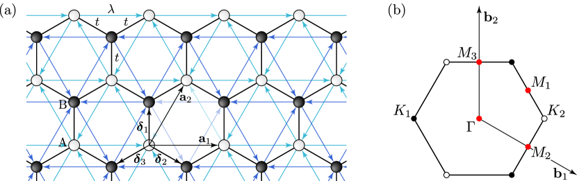
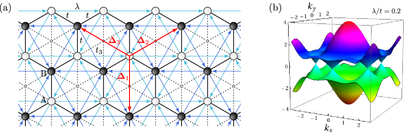
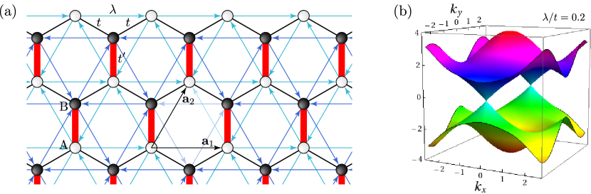
The Kane-Mele (KM) model was derived as a model with an intrinsic spin-orbital interaction on a two-dimensional honeycomb lattice – the structure of graphene. The model with its lattice structure and parameters is illustrated in Fig. 1(a). The idea proposed by C. Kane and E. Mele was to construct a spinful model which consists of two copies of the the Haldane model[43] with opposite spin.[6, 7] Although the spinless Haldane model alone breaks TRS, the spinful KM model is time-reversal invariant. The Hamiltonian of the KM model is given by,
| (1) |
where , , denote the spin species and . The first term describes the nearest neighbor hopping on a honeycomb lattice. The second term represents spin-orbit coupling, it connects next-nearest-neighbor sites with a complex (time-reversal symmetric) hopping with amplitude . The factor depends on the orientation of the three nearest neighbor bonds the electron traverses in going from site to and affects the orientation of the next-nearest-neighbor bonds for one spin species. As shown in Fig. 1(a), if the electron makes a left (right) turn to get to the next-nearest-neighbor site. The in the spin-orbit coupling term is the z-component of the Pauli matrix, which furthermore distinguishes the and spin states with opposite next-nearest-neighbor hopping amplitude; thus the next-nearest-neighbor hopping is spin-dependent. Physically, the term stands for the intrinsic spin-orbit coupling, where is conserved, and amounts to a staggered spin-dependent magnetic field threading the triangular plaquettes defined by the next-nearest-neighbor bonds.
To better understand the KM model, we Fourier transform the Hamiltonian in Eq. (1) into momentum space. In terms of the spinor , Eq. (1) is recast as in basis of and expressed in a block-diagonal form as
| (2) |
Here, comes from the nearest neighbor hopping and represents the spin-orbit interaction. Each of the block diagonal matrices represents a Haldane model for one spin species.[43] Although individually breaks the TRS, the whole Hamiltonian in Eq. (2) recovers it at the time-reversal invariant momenta . The argument is given as follows: consider the time-reversal operator , where is the Pauli matrix applied in the sublattice space and denotes the complex conjugation operator.[12, 20] Application of to a single-particle Bloch state means to invert the momentum from to , flip the spin from to , and the complex conjugate is to be taken. By interchanging the and sectors of Eq. (2), taking the complex conjugate and considering , as well as , one can verify that . Thus, the KM model is time-reversal invariant only while , i.e., at the TRIM.
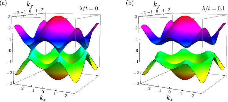
At , Eq. (2) gives rise to the famous graphene band dispersion , in which the conduction bands and valence bands touch at the Dirac points [filled and open circales in Fig. 1(b)]. Around the Dirac points the band dispersion is linear and forms Dirac cones. The band structure of the graphene dispersion is depicted in Fig. 2(a). At half-filling, i.e., the number of electrons equals the number of lattice sites, the Fermi level is located exactly at the Dirac points and the system is gapless with a vanishing density of states and is hence a semi-metal.[44]
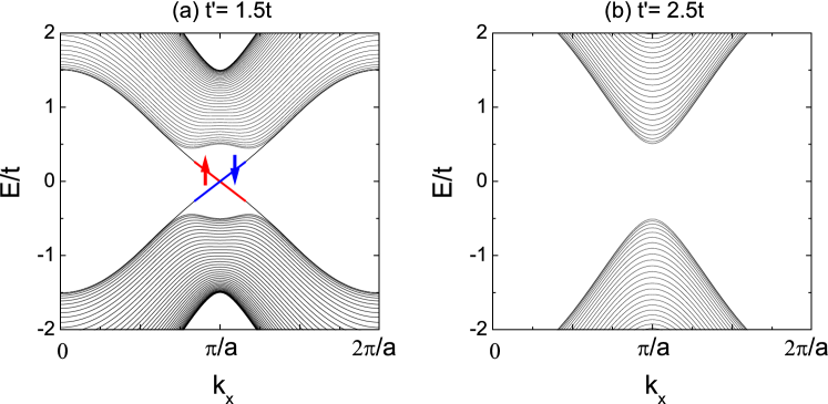
Any finite opens a bulk gap. Figure 2(b) show the case of . Since the KM model Hamiltonian can be decoupled as two independent Hamiltonian , the dispersion of the KM model can be easily solved as , each of them is double degenerate. The bulk gap at the Dirac points opens as .[20] Note that the inversion symmetry breaking field, e.g., a staggered potential term , where () on sublattice A (B), also opens a gap. Hence topological trivial and nontrivial insulators cannot be easily distinguished by the bulk gaps. The KM model however features the hallmark of protected edge states once a boundary is introduced into the system according to the bulk-edge-correspondence in non-trivial topological systems.[29, 31] The edge state of the KM model can be seen by solving Eq. (1) on a ribbon geometry.
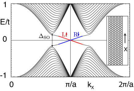
Figure 3 shows the one-dimensional band structure for a zigzag ribbon (as shown in the inset).[6, 45] In the projection onto the one-dimensional edge, one can see the bulk band gap at the and points as indicated by the arrows. There exist two bands within the band gap, which connect the and points. These transverse modes are states localized on the edges of the zigzag ribbon, which is analogous to the chiral modes localized on the edge of the IQH state. Here however, the electrons with and spin states propagate in opposite directions along one edge; thus it is bidirectional and the net charge carrier is zero. The bidirectional channels however bring a nonzero spin current ,[7] and the spin Hall conductivity characterizes that the magnitude of spin currents are carried by the opposite spin components on the edges. The edge states are named helical state[19] and are essentially one dimensional chiral Dirac fermions which occurrence is contingent on the properties of the two dimensional bulk system. This so-called bulk-boundary correspondence states the fact that the existence of edge states is guaranteed by the topological nature of the bulk system and the two are inextricably linked with each other. This spin-filtered state is topologically different from an ordinary one-dimensional metal, where the electronic behavior is not spin-filtered.[45] Note that the helical states cross at , and are hence protected by the time-reversal symmetry. This means that the edge states are also robust against time-reversal symmetric impurities.[19] The number of pairs of edge states (modulo 2) is directly linked to the value of the topological invariant .[6, 29] The protection of the topological state with respect to adiabatic deformations implies that the only way to achieve a change of the topological invariant is to close the bulk band gap. Hence, investigation of edge properties can be used to identify the corresponding properties of the bulk. Note that the statement above is valid as long as the invariant is well defined. Indeed, the topological properties of a system can be changed without closing the bulk gap in the single-particle spectrum.[46, 47, 48] However, in an interacting system beyond the mean-field approach the spontaneous symmetry breaking associated with a direct transition from a topological insulator to a topologically trivial phase is always accompanied by the closing of a gap, albeit in the charge-, or spin-sectors.[27]
As mentioned previously, Eq. (2) consists of two Haldane model copies for each spin species, and each of them provides an IQH state with the quantized Hall conductivity . In close analogy to the IQH effect, the QSH insulator has a quantized spin Hall conductivity, , showing the nontrivial topological feature. Each spin species contributes a nontrivial Chern number . The time-reversal symmetry guarantees that the Chern numbers for the two spin sectors have opposite signs . Therefore, we have the net charge Chern number , but a nonzero , which defines the quantized spin Hall conductivity in terms of and has been shown to be robust against time-reversal symmetric disorder and magnetic Kondo-Impurities.[45, 49, 50, 51] Although a nonzero value in indicates the nontrivial topological property, is however not necessarily quantized.[7, 45] For example, in the presence of the Rashba coupling
| (3) |
which preserves the time-reversal symmetry, but breaks inversion symmetry and causes to be no longer conserved, the spin Hall conductivity will deviate from quantization and can take continuous values.[49, 50] Nevertheless, as long as the band gap remains open, the system with finite remains a QSH insulator. Consequently, the spin Hall conductivity does not constitute a topological invariant for the QSH state. Instead, the topological invariant of the QSH state is the invariant, which is given by
| (4) |
and takes on the values of 0 or 1. The value corresponds to the topologically nontrivial QSH state and corresponds to a topologically trivial insulator.[7, 29, 31] The authors of Refs. \refciteKane05b,Kane2007 have shown that even in the presence of finite (below the threshold value which closes the bulk gap), and therefore the invariant is indeed a proper description to distinguish the QSH regime from a topologically trivial insulator.
2.2 Quantum Monte Carlo Simulations & the Kane-Mele-Hubbard Model
Next let us turn to the QSH state under the influence of interactions. The KM model in Eq. (1) is non-interacting. To consider electron interactions, the simplest non-trivial approach is to augment the KM model by an additional on-site Coulomb repulsion of strength , which results in the Kane-Mele-Hubbard (KMH) model given by
| (5) |
The KMH model is a many-body Hamiltonian which can no longer be diagonalized via a Fourier transformation. In order to study the topological nature of the KMH model in the presence of interaction, we need to employ more advanced techniques. At half-filling, the bipartite nature of the KMH model sports particle-hole symmetry and TRS, so that QMC simulations can be employed to solve this system in a controlled and unbiased way on large lattices. In this section, we briefly introduce the determinant QMC technique which is used to study the KMH models in following sections. For more detailed description, we encourage readers to refer more specific articles.[52, 53]
The determinant QMC has been shown to be an excellent and unbiased approach to deal with strongly correlated system with Hubbard interactions.[54, 55, 56, 57, 58] In the zero temperature ( projector algorithm, the ground state wave function can be obtained by stochastic projection of the Hamiltonian onto a trivial wave function , provided a finite overlap . For the KMH model, the lowest single-particle state of is a good candidate for the trial wave function . The expectation value of an arbitrary observables is obtained by
| (6) |
The imaginary time axes is discretized into Trotter-slices such that the projection operator for , with the projection length and . Using the first order Suzuki-Trotter decomposition, can be decomposed as
| (7) |
The interaction term is non-bilinear in the fermionic operators and cannot be expressed in the single-particle basis. However, the discrete SU()-invariant Hubbard-Stratonovich transformation,[53] allows to transform the interacting imaginary time-evolution operator into bilinear form at the cost of the integration over a four-component auxiliary field on all sites.
| (8) |
where
| (9) |
The systematic error of the Hubbard-Stratonovich transformation of order is still small compared to error introduced by the asymmetric Suzuki-Trotter decomposition Eq. (7) and can be controlled by choosing appropriately small values for . In most of the QMC simulations in the upcoming sections, we employ .
The integration over all auxiliary field configurations is performed using stochastic Monte Carlo sampling. The partition function is given by
| (10) | |||||
Here, a trial wave function which corresponds to the non-degenerate ground state of a single-paritle Hamiltonian with , where is the corresponding non-degenerate ground state energy. We usually choose , with being a statistically irrelevant small magnetic flux threading the KM model on the torus in order to lift its degeneracy.[52, 53, 27] The sum runs over possible auxiliary configurations , where , . The weight explicitly reads
| (11) |
with and for .
In order to have QMC simulations free of the negative sign problem the configuration weights must remain positive definite. In the half-filled KMH model, TRS and particle-hole symmetry yield the condition . To demonstrate this is fulfilled in the KMH model one just needs to check that the nearest-neighbor hopping matrix elements, the spin-orbit hopping matrix elements and the interaction matrix elements in Eq. (10) indeed render such a property. As for the nearest-neighbor hopping, it is spin independent, such that
| (12) |
and bipartite hopping matrix elements are real numbers and will automatically give if there are no other terms in the Hamiltonian. The spin-orbit hopping matrix elements have a complex hopping amplitude, but are complex conjugate with respect to by construction, hence
| (13) |
satisfies the condition as well. At half filling , so that the interaction term has the same property:
| (14) |
Hence, the interaction matrix element for spin is the complex conjugate of the interaction matrix element for the other spin . Consequently, one can readily see that the nearest neighbor hopping matrix elements, the spin-orbit hopping matrix elements and the interaction matrix elements all guarantee and hence the configurational weight is indeed real and positive definite. The QMC simulations of KMH model at half-filling are therefore free of the sign problem.
Without sign problem, the QMC method allows to efficiently measure equal-time and time-displaced correlation functions, such as the single-particle Green’s functions[57, 59, 60]
| (15) |
The single-particle gap can be then determined from the long imaginary time behavior of the time displaced single-particle Green’s function, i.e., . For the KM model at half-filling the relevant momenta are at the Dirac points and . The uniform single-particle gap obtained from is used to describe the single-particle gap, independently of a specific momentum. The gap for spin excitations is obtained similarly from the imaginary-time displaced spin-spin correlation function, for example in the antiferromagnetic ordering (staggered) sector,
| (16) |
The double brackets denote the cumulant of a correlation function of operators . The spin gap are obtained from . Antiferromagnetic order in the honeycomb lattice corresponds to the momentum at , hence, . As for the static antiferromagnetic structure factor, it can be obtained directly from the equal time (static) spin-spin correlation function in the staggered sector at the momentum point . Note, that the intrinsic spin-orbit coupling term breaks the SU(2) spin rotational invariance down to the U(1) symmetry group, such that for spontaneous spin symmetry breaking will occur in the transversal spin channel.[20, 25, 26, 27] Hence it is necessary to monitor - and -spin correlations independently.
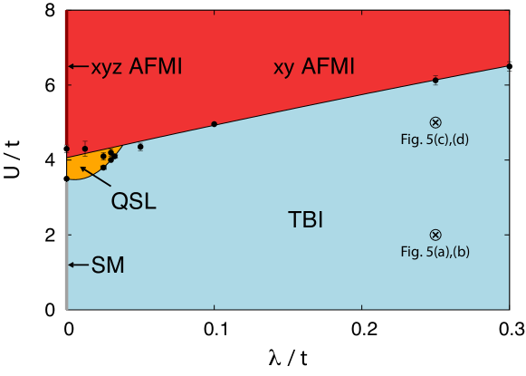
Figure 4 shows the phase diagram of KMH model at half-filling obtained from QMC simulations.[25, 26, 27] Along the axis, where there is no spin-orbit coupling, the system is a semimetal at small interaction with Dirac points shown in Fig. 2(a), and is an antiferromagnetically order Mott insulator at large with Heisenberg type order ( AFMI). The existence of the phase in the intermediate interaction strength (a possible quantum spin liquid state) and the nature of the semi-metal to antiferromagnetic insulator transition is under intensive debate.[57, 58, 61] For any finite , the system is in the QSH state, here named as topological band insulator (TBI). At finite interaction , the system (indicated by blue region) is adiabatically connected to the noninteracting case, e.g., the KM model. A stronger interaction (i.e., at , ) will drive the TBI through a continuous quantum phase transition into an antiferromagnetic ordered Mott insulator (AFMI). The single-particle gap remains open, but the spin gap closes. At finite , the SU(2) spin symmetry is already broken down to U(1) such that the magnetic order in the strong coupling regime is in the plane (easy plane) of spin space. The transition from TBI to the AFMI has been shown to be consistent with the 3D XY universality class.[27]
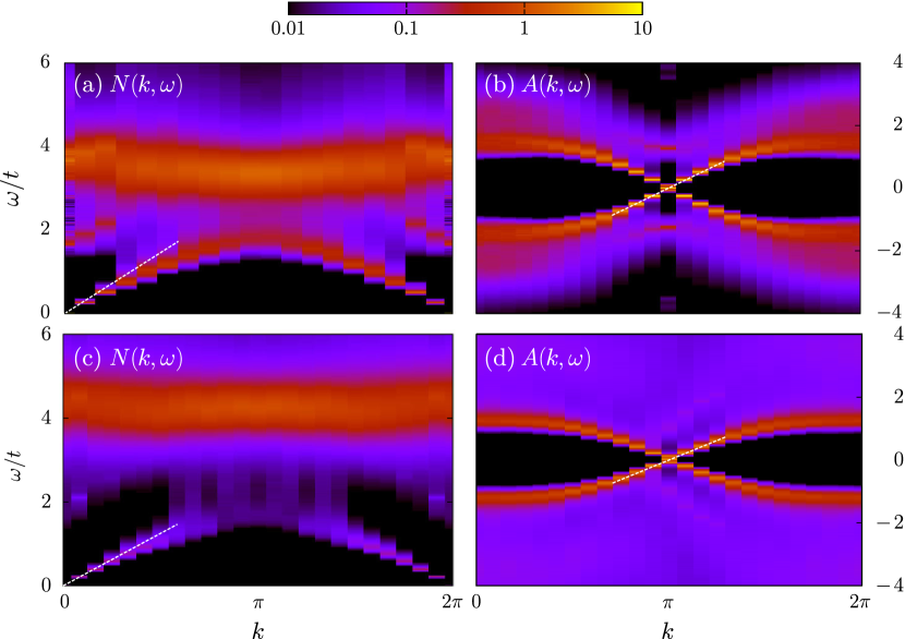
To explore the correlation effect on the time-reversal symmetry protected edge states, the authors in Ref. \refciteLang2011 studied the KMH model on the zigzag ribbon (as shown in the inset of Fig. 3), and obtain the spectral information along the zigzag edge of the ribbon. Figure 5 shows how the edge states evolve in the TBI phase under the increasing influence of correlations. The panels show the single-particle spectral function
| (17) |
and the dynamic charge structure factor
| (18) |
along the ribbon edge of an open system. At small interaction strength [panels (a) and (b)] signatures of the edge states can be clearly seen below the bulk gap as linear mode around . However, as the interaction strength approaches the critical value, i.e. in panels (c) and (d), one observes a strong depletion of spectral weight in the low-lying charge modes in (c), which leads to reduction of the Drude weight. As the interaction strength is still below above which the transverse antiferromagnetic order sets in, despite strong correlations, the single-particle spectrum (d) still exhibits the helical edge states, which remain essentially unaffected by the increased correlations.
3 Detecting Topological Orders
As discussed in Sec. 2, the quantity to distinguish the QSH state from a trivial band insulator is the invariant. Physically, the topological invariant is associated with the change in the time-reversal polarization when a magnetic flux is threaded through a cylinder geometry varying from to .[38, 45] Though this picture was initiated in the noninteracting limit, with interaction one can still observe similar behavior. In Sec. 3.1, we shall show that, in the KM model the insertion of -fluxes gives rise to a Kramers doublets of spin-fluxon states.[37] We then move our discussion to the evaluation of the invariant. Here, likewise, the construction of the topological invariant was also initially defined in the noninteracting limit.[7, 12, 38, 45] The invariant, however, can be straightforwardly generalized to interacting cases[40, 62] and can be expressed in terms of single-particle Green’s functions. An overview of to the index and the parity behavior of the single-particle Green’s function will be provided in Sec. 3.2. To illustrate the formalism and demonstrate its power, in Sec. 3.2.2 we investigate the interacting topological phase transitions in two descendants of the KMH model within QMC simulations, the generalized KMH model[39, 41] and the dimerized KMH model. [42] Moreover, we point out the limitation of the topological invariant approach in the QMC method. Sec. 3.2.3 will render an example which illustrates the invariant’s shortcoming to describe quantum phase transitions which involve spontaneous symmetry breaking as a consequence from collective excitations. Finally, in Sec. 3.3 we will discuss the evaluation of the spin Chern number from the sum over real-space derivatives of products of the eigenvectors of the zero-frequency Green’s functions.[39]
3.1 -flux Insertion
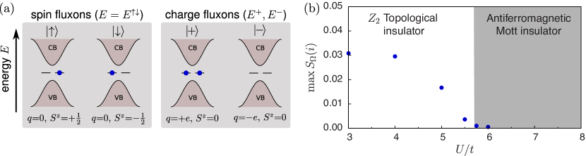
The authors of Refs. \refciteRan2008 and \refciteQi2008 have shown, that on a lattice with periodic boundaries, -fluxes can be inserted in pairs, threading selected plaquettes of the lattice. In the topological phase, each -flux gives rise to four fluxon states near the corresponding flux-threaded hexagons. The states correspond to the spin fluxons , , forming a Kramers pair related by time reversal symmetry, and charge fluxons , , related by particle-hole symmetry as illustrated in Fig. 6(a). As a consequence of the bulk gap, these states are exponentially localized around the flux-threaded plaquettes and energetically lie inside the bulk band gap.
Assaad et al.[37] have successfully shown, that two maximally separated -fluxes can be used to probe the correlated quantum spin Hall state for its topological properties. The -flux pairs introduce edges in the bulk system around which these spin fluxons manifest. Spin fluxons can then be detected by calculating the lattice-site-resolved, dynamical spin-structure factor at zero temperature, defined as
| (19) |
Here, corresponds to the spectrum of spin excitations at lattice site , defines the excitation energies and denotes the ground state. The dynamical spin-structure factor picks up the spin-fluxon states. Integration of up to an energy scale well below the charge gap , allows to account for all spin-fluxon excitations. This yields the site resolved integrated dynamical structure factor , which can be used to identify the presence of spin-fluxons in the topological insulator, or lack thereof in topologically trivially ordered phases. The dependence of is demonstrated in Ref. \refciteAssaad2013 for the KMH model across the magnetic quantum phase transition from TBI to the AFMI at . In Fig. 6(b) the maximum of is plotted as a function of the interaction strength . The observable acquires finite values in the topological-insulator phase, and a strong drop is observed on approaching the critical point , before it vanishes in the magnetically ordered phase. The spin-fluxon signal can be used in quantum Monte Carlo simulations as a general tool to distinguish topological and nontopological phases, although the need for the continuation to real frequencies can make its use impractical, or result in lack of accuracy.
In addition to the integrated dynamical structure factor at , at finite temperature spin fluxons created by -fluxes give rise to a characteristic Curie law in the spin susceptibility, which can be used to identify topological properties in finite temperature quantum Monte Carlo simulations. At low temperatures, the spin susceptibility then follows the form , or per -flux. For details on further results of -fluxes and the interactions between the induced spin fluxons we refer the reader to Ref. \refciteAssaad2013.
3.2 The Topological Invariant
3.2.1 The Parity Invariant and the Zero-frequency Green’s Function
The QSH (topological insulator) state is identified by the invariant . In Refs. \refciteFu2007prb,Fu2006prb, the invariant is defined as
| (20) |
where denotes the time-reversal invariant momenta (TRIM) of the Brillouin zone. In two dimensional QSH states, there are four TRIM points, whereas in three dimensional topological insulators there are eight. For the honeycomb lattice, the TRIM have been introduced in Fig. 1(b). The value of the number is evaluated according to Ref. \refciteFu2006prb as
| (21) |
Here, is an antisymmetric matrix with the elements defined by and , stand for the band indices. denotes the time-reversal operator, for spin-1/2, and is the Bloch state of the noninteracting Hamiltonian of Eq. (2), i.e., . Pf denotes the Pfaffican function of the matrix , with . Note that due to the presence of the square root, the sign of is ambiguous. should be chosen continuously in the Brillouin zone, so that is defined globally.[12]
In the presence of inversion symmetry, which is the case for the KM model without Rashba coupling, Eq. (21) can be simply evaluated as[12]
| (22) |
where denotes the parity eigenvalue of the -th occupied band at momentum . Here we used to indicate that there exists the Kramers degenerate pair and with the same parity value. For sustained inversion symmetry, the Bloch states are also eignestates of the inversion operators, so . Rather than Eq. (21), Eq. (22) is obviously more practical and simpler to evaluate the invariant.
Equations (21) and (22) are only suitable in the noninteracting limit. In the presence of interaction, the Bloch states are no longer well-defined. However, it has been shown that for interacting topological insulators the topological order parameters can be expressed in terms of Green’s functions defined in the extended frequency-momentum space[65]
| (23) |
in which , . The momentum are integrated over the Brillouin zone and the frequency is integrated over . The extra dimension in has the following meaning: corresponds to the Green’s function for interacting topological insulator, corresponds to the Green’s function of a trivial insulator. Values of smoothly connect the two limits. Equation (23) can be interpreted as the physical response of an insulator in the topological field theory.[66] This formula however involves the full frequency-momentum space integral and an extra-dimension where one extends the topological insulator to a topologically trivial insulator. Thus it is apparently not practical to implement this formula in numerical simulations. Fortunately, the authors of Ref. \refciteWang2012prx showed that is topologically equivalent to the nonzero frequency Green’s function , and hence this topological order parameter can be simply expressed in terms of the Green’s function at zero frequency.[40, 62, 67] is further interpreted as the topological Hamiltonian, which contains all necessary information of the existence of surface states.[68] This greatly simplifies numerical and analytical calculations.
The procedure to obtain the topological invariant from the zero-frequency Green’s function is hence described as follows: Diagonalize the inverse zero-frequency Green’s function at the TRIM
| (24) |
to acquire the state , and choose the eigenvectors associated with positive eigenvalues (, denoting the generalization of it occupied bands and are called right-zero, or R-zero).[40] The R-zeroes span the R-space at each . In analogy to Eqs. (21) and (22), for an interacting topological insulator with inversion symmetry we have
| (25) |
The matrix elements . In inversion symmetric systems is the simultaneous eigenvector of and the parity (or inversion) operator
| (26) |
This means the evaluation of the (parity) invariant only relies on the structure of the zero-frequency Green’s function , which can be readily computed within auxiliary field QMC simulations.
In order to compute the Matsubara Green’s function from the imaginary-time displaced Green’s function, and continue in particular to zero frequency, let us first consider the system at a finite temperature . The finite temperature, imaginary time Green’s function with , is a matrix expressed as
| (27) |
where A, B are sublattice indices of the honeycomb lattice. To be represented in Matsubara-frequencies , one needs to perform the Fourier transformation
| (28) |
The particle hole symmetry of the half-filled KMH model, i.e., under the transformation in each spin sector together with inversion symmetry leads to the following conditions on : For equal sublattices, , while, for , . We thus obtain for the diagonal elements of the Green’s function at one of the TRIM points
| (29) |
and, for ,
| (30) |
Now, the limit can be taken properly: From the projective QMC simulations, we obtain the ground state Green’s function , and then perform the above integrals with a sufficiently large cutoff , set e.g. by the imaginary time evolution length of the Green’s function employed in the QMC simulations (we usually use ). Note, that one cannot simply take the limit before accounting for the (anti)symmetry conditions on the imaginary time Green’s functions. This would lead to wrong results, as exemplified below. After (anti)symmetrization, the limit can be performed with the Green’s functions, so that
| (31) |
and, for ,
| (32) |
Note, that this structure of the Green’s function is a direct consequence of the common eigenvector system shared by , and with , such that the one has the relation
| (33) |
Hence, within the QMC simulations, one merely needs to measure the off-diagonal part of the Green’s function explicitly. To illustrate the above point, consider the exact imaginary-time Green’s function
| (34) |
If calculated naively, via , one would (wrongly) obtain a finite value of instead of the actual value (i.e. zero).
The KMH model has the explicit conservation of the Hamiltonian (spin independent motion). Thus the single-particle Green’s function is block-diagonal in spin-space , and the procedure of calculating in Eq. (26) can be restricted to , or . The Green’s function is a matrix in the A/B-sublattice basis. In the spinor convention , the parity operator of the honeycomb lattice is defined as ,[12] which interchanges A and B sublattices. Note that since and have the same eigenvectors, we can directly diagonalize instead of the inverse Green’s at the TRIM
| (35) |
and then choose the R-zero eigenvectors () to evaluate the corresponding parity . For the honeycomb lattice, at half filling, thus each has one R-zero and we can simplify the notation . Also at these TRIM, Kramers degenerate partners share the same parity eigenvalues and one can restrict the procedure to one spin sector, say , to compute , and then
| (36) |
The value of denotes a trivial insulator, whereas indicates a topological insulator. In the following section, we will present two example cases to identify the interacting QSH state using Eq. (36).
We will show in Sec. 3.2.2 that in addition to the invariant, the proportional coefficient in Eq. (33) can also be used to characterize the topological insulator/trivial insulator phase transition and even is more sensitive than numerically: at the topological phase transition, where the bulk gap closes at the TRIM, the zero-frequency single-particle Green’s function is divergent on the poles and flips the sign beyond the transition.[69] Here we want to point out, that while in the KM model (), , in the cases of finite and for interacting Green’s functions is not guaranteed in a single QMC measurement (cf. the supplemental material of Ref. \refciteHung2013). The well-defined parity invariant is recovered only by acquiring sufficient statistics within the QMC simulations. In the following we present cases, where this approach works, or breaks down respectively, and discuss the limitations of the use of the invariant in simulations.
3.2.2 Topological Phase Transitions in the Generalized and the Dimerized Kane-Mele-Hubbard Models
In this subsection, we will present two example case studies of calculating the parity invariant and the spin Chern number within the QMC method. The models considered are descendants of the KMH model, which we called the generalized KMH model[39, 41] and the dimerized KMH model.[42] Both of the models characterize a -topological insulator to trivial-insulator phase transition as a function of the tight-binding parameters. Following Sec. 2.2, at half-filling both systems are particle-hole and time-reversal symmetric. Therefore the QMC simulations in these models are sign-free and we can accurately determine the topological phase boundary at different values of beyond the mean-field level.
The main results are that, in the generalized KMH model, increasing stabilizes the topological insulator phase, whereas the correlation effects in the dimerized KMH model destabilizes the topological insulator phase. In both cases the invariant proves to be a practical tool to determine the loss of the topological nature as the systems are tuned into trivial band insulators. Similar to the KMH model in Fig. 4, the onsite Hubbard interaction in the descendant KMH models in the thermodynamic limit will also induce spontaneous planar antiferromagnetic order which breaks inversion symmetry, such that Eq. (36) is no longer well-defined. Across the transition into the antiferromagnetic state on finite size lattices the invariant however fails to reflect the change of the topological nature of the phases. The recovery of its validity in the thermodynamic limit is not obvious from the results obtained for increasing system sizes.
Generalized Kane-Mele-Hubbard model
The generalized Kane-Mele model (GKM) is considered on the KM lattice with real-valued third-neighbor hopping
| (37) |
sums over third-nearest-neighbor hoppings described by vectors: , and , with the hopping amplitude of connecting and sublattices as indicated in Fig. 7(a). At , the GKM model reduced to the KM model, and thus it is a topological QSH state.
In momentum space, the GKM model can be recast as , with
| (38) |
The off-diagonal term is given by , where comes from the KM model in Eq. (2). Since the hopping does not break the time-reversal symmetry, the GKM Hamiltonian is still time-reversal symmetric. The dispersion of the GKM model is given by .
Beginning from and then moving to larger , the GKM model remains gapped, until at , the gap collapses. This indicates that a topological phase transition occurs at , and the regime of is a QSH state since it adiabatically connects to the case. We have confirmed that the system in this regimes has . The band structure of Eq. (38) at is shown in Fig. 7 (b), where the system exhibits three gapless modes located at the three TRIM and , rather than the Dirac points . On the other hand, as , the band gap opens again, and it is identified as , a trivial insulator. At the noninteracting level, the value of is independent of .
To further understand the discrepancy between the topological band insulator phase and a trivial insulator phase, one can study the edge modes with a zigzag ribbon geometry. Figures 8(a),(b) reveal different behavior of the edge spectra for topologically nontrivial and trivial cases at . For the topological insulator phase at , Fig. 8(a) shows an odd number of helical edge states within the band gap, crossing at the time-reversal invariant point .
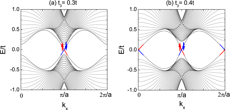
At however, Fig. 8(b) shows an even number of helical modes at and , and thus from the perspective it is a topologically trivial state (the edge states are not topologically protected). However, note that the two helical states imply that the spin Chern number (discussed in Sec. 3.3) , and each spin sample is a IQH state. From the tight-binding calculation, we determine that at , whereas at for . This corresponds to the observation that the bulk band gap closes at three TRIM in Fig. 7(b) ().[39]
Next we augment the GKM model with an onsite Coulomb interaction. This generalized KMH model is the GKM model plus an onsite Hubbard interaction, i.e., with . By sign-free QMC simulations, we can demonstrate how to identify a correlated topological insulator phase and a trivial insulating state with the single-particle Green functions and the index. The simulations are performed using an imaginary time step and an inverse temperature . All the results use the periodic boundary conditions and the number of sites is , where is the linear system size.
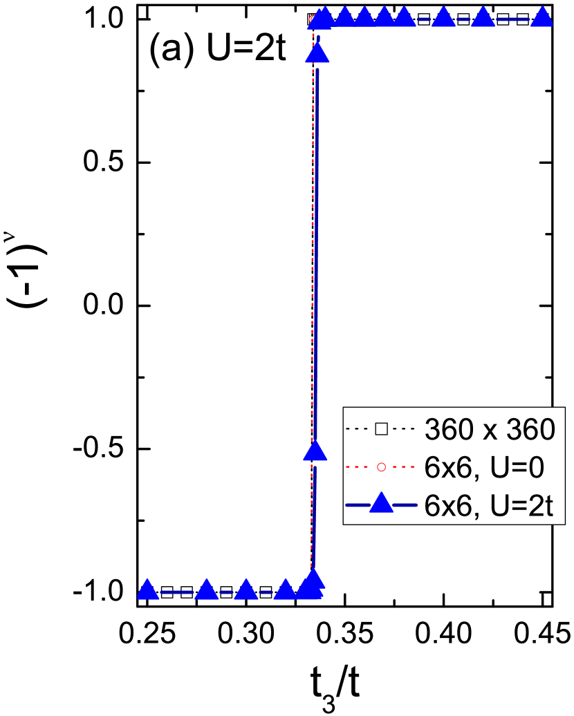
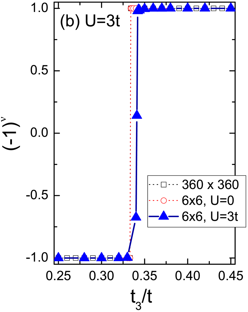
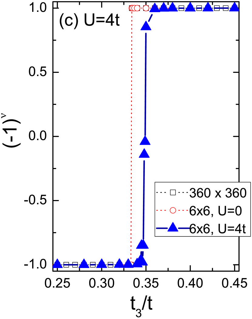
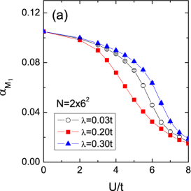
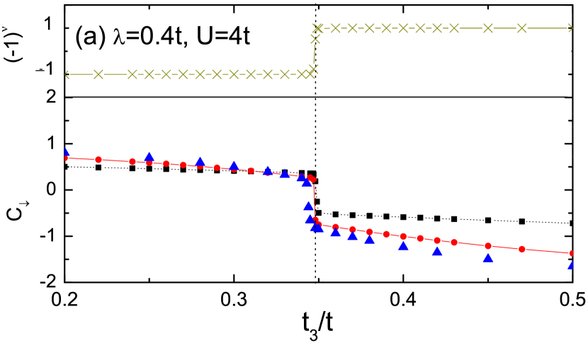
For the noninteracting case with , the critical value separates topologically non-trivial and trivial phases. In Figs. 9, we present the invariant as a function of for different values of for on a cluster. Open and solid symbols denote the noninteracting and interacting cases, respectively. For comparison, we also show the noninteracting () invariant from QMC simulations on a cluster (open red circles) and from tight-binding calculations on a cluster (open black squares). Both results show that the invariant varies at , and confirm the accuracy of our small-size QMC calculations in the noninteracting limit. In the topological insulator phase (), only the point is parity odd (); the other three TRIM are parity even (), so and . Across the transition upon increasing , change parity. and are parity even, whereas, are parity-odd, so and .
Next let us turn to observe the interacting case (). In order to avoid invalidating Eq. (36), we properly choose the value of without inducing the magnetic ordering. For , we numerically confirm that in the regime of , is still below the critical interaction.[41] The blue solid triangles in Figs. 9(a)(c) depict the dependence of the invariant on . In the presence of electronic correlations, the parity properties of the TRIM still remain, and Eq. (36), to evaluate the invariant, remains well defined. This is because at moderate interaction the system adiabatically connects to the QSH state, as long as the band gap remains open. Note that here is determined over thousands of QMC configurations, with small statistical errors. At weak interaction, , the phase boundary is estimated at , which only slightly deviates from the noninteracting . By increasing , however, one can explicitly see that the critical points start to move towards larger values, indicating that the topological insulator phase is stabilized by the interactions. At and , the critical points are estimated at and , respectively. This indicates that a slight shift () of the topological phase boundary is driven by the Hubbard interaction. This is in contrary to the correlation effects in the dimerized KMH model which we shall discuss later.
It is interacting to note that, such a boundary shift originates from quantum fluctuations, since no shift as a function of is observed in a static Hartree-Fock mean-field approximation. As long as without inducing the antiferromagnetic ordering, the Hartree-Fock result is the same as the tight-binding calculation. Therefore, the QMC results can efficiently capture the quantum fluctuations originating in the interactions and one can study the topological phase under electronic correlation accurately.
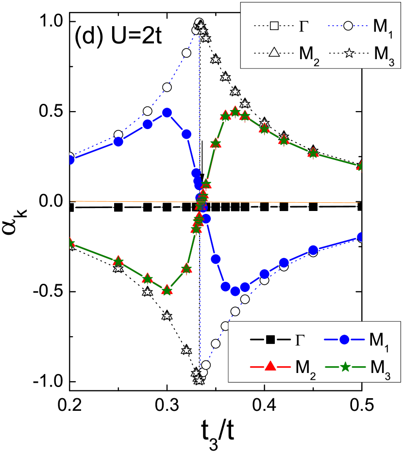
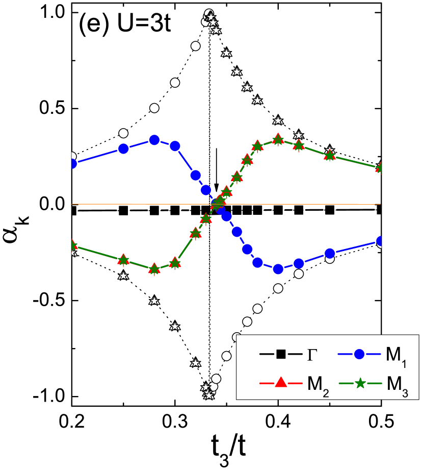
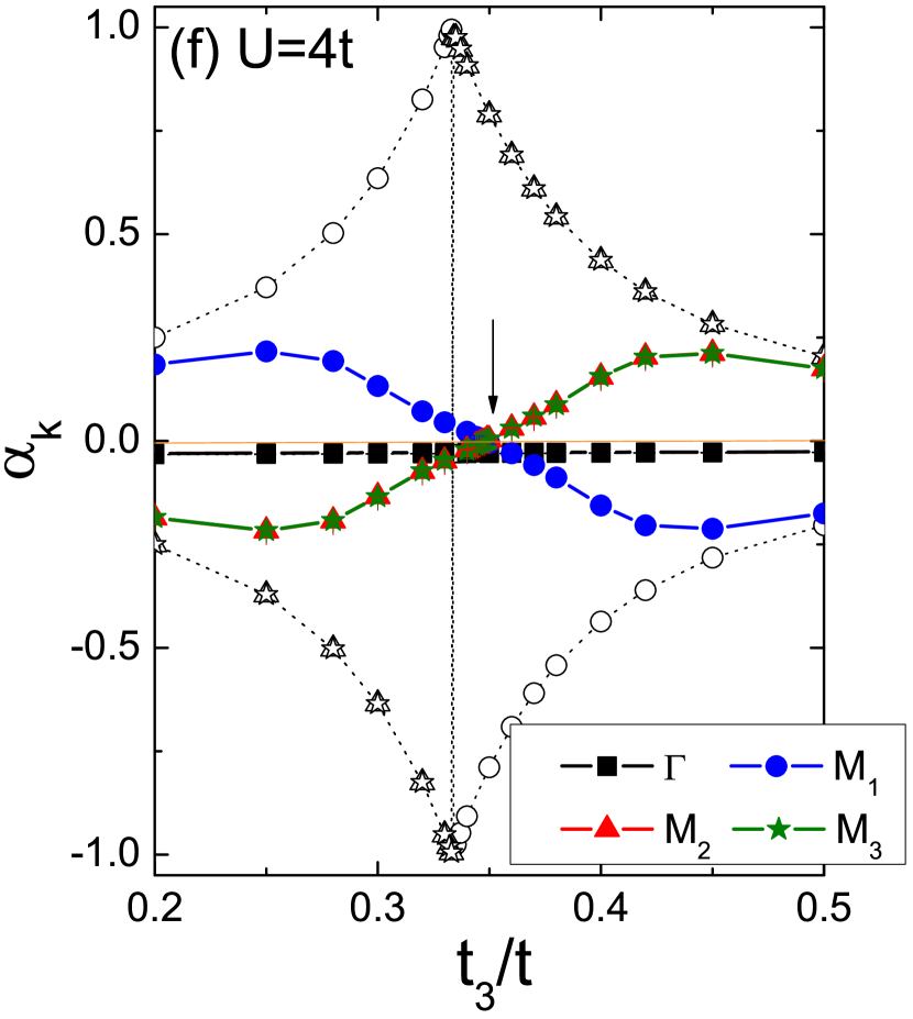
Next, we investigate how the single-particle Green’s function behaves during the topological phase transition. In the inversion symmetric generalized KMH model, at the TRIM, the zero-frequency Green’s functions for each spin can be simply expressed in terms of as [cf. Eq. (33)]. In Figs. 9(d)(f), we show the proportionality coefficient as a function of for finite . For comparison, in the noninteracting case is also depicted. At , we find the universal relations, and , for all values of and . The values of (denoted by black hollow squares, covered by the solid squares) behave smoothly as passes through . However, ’s of the other TRIM are divergent at and change signs at the topological phase transition. This can be realized that at a critical point, the gap closes at the TRIM, so the zero-frequency Green’s functions behave divergently on the poles and then change signs.[69] For any and at , the location of the sign change is always at , implying that the behavior of can be another indication to determine the topological phase transitions, like the invariant.
Similarly, turning on the Hubbard interaction , one can still observe the sign change in at the topological phase transitions. For finite , within QMC simulation errorbars the zero-frequency Green’s functions retain their -like form, and the universal relations and still hold, independent of the value of . However, the positions where ’s change signs move away from . In Figs. 9(d)(f), the arrows label the location of the sign changes in , indicating the topological phase boundaries in the interacting case. Clearly, compared with the upper panels, Figs. 9(a)(c), the locations for the sign change are consistent with the places where the invariant jumps.
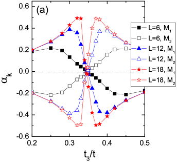
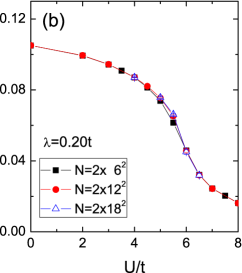
In Figs. 9(d)(f), one can also observe how the coefficients evolve upon increasing interactions. At larger , the magnitude of is more suppressed. Although the sign change is still evident, the sign-flip behavior becomes more smooth with stronger interaction. This corresponds to a smeared phase boundary indicated by the invariant changes in Figs. 9(a)(c). Such an effect, however, will become less important upon increasing sizes. Figure 10(a) shows the size dependence of the coefficients at versus . The spin-orbital coupling and interaction are fixed at and . Note that has opposite parity to , so the coefficients have opposite sign at these momenta. Upon the topological phase transition, both flip signs. However, one can see that upon increasing sizes, the behavior of near the is getting divergent, which is observed in the noninteracting limit.
In addition to the values of , one can also observe a weak finite-size dependence on the locations of sign flip. This implies that considering small clusters is able to identify the topological phase transition. Interestingly, away from the topological phase transitions, e.g., and , the coefficients for seem to be consistent with the noninteracting values. Therefore, interaction effects in are most apparent as approaches the topological phase transition.
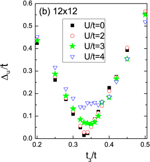
Besides the invariant and associated the Green’s function behavior, monitoring the closing of the single-particle gap is also another possible indicator for the topological phase transition. However, the single-particle gap is subject to a stronger finite-size effect. Figure 10(b) shows for a fixed system size , that at and , one can clearly see the vanishing gap location. At the behavior becomes less obvious but the minimum gap location is still visible. Furthermore at , the plot cannot provide clear information to identify the location of the topological phase transition. While this observation could be systematically improved by performing finite-size analysis, it is clear that the behavior of the single-particle gap is not as sensitive as the topological invariant, since large lattices are needed in order to perform reliable finite-size scaling.
Dimerized Kane-Mele-Hubbard model
Complementary to the the above mentioned GKM model, it has been shown that the KM model with anisotropic nearest-neighbor hopping can also exhibit a topological phase transition into a trivial band insulator.[42] This is the so-called dimerized Kane-Mele (DKM) model and its Hamiltonian is given by
| (39) |
Different from the GKM model, the DKM Hamiltonian only contains nearest-neighbor hopping. However, one of the three nearest-neighbor hoppings is chosen with a different amplitude along the direction compared to the other two along the directions, as shown in Fig. 11 (a).
The Hamiltonian in momentum space can be written as , with
| (40) |
The off-diagonal term is different from the corresponding term in the Kane-Mele Hamiltonian in Eq. (2) due to the anisotropic nearest-neighbor hopping . It is given by . The DKM Hamiltonian is also time-reversal symmetric, since Eq. (40) it block diagonal in spin space, and and . The dispersion of the DKM system follows from the eigenvalues of and is given by .
As discussed in Sec. 3.2.1, the topological invariant is identified by the zero-frequency Green function at the four TRIM , and is calculated according to Eq. (36) from any of the two spin sectors, which together form a Kramer’s pair at each TRIM. In the noninteracting case, , we obtain for finite values of spin-orbit coupling , a change in the invariant from for to for . This indicates the topological phase transition from a topological insulator (the QSH insulator) to a trivial band insulator exactly at . As shown in Fig. 11(b), at , the single-particle gap closes at the point [compare with Fig. 2 and Fig. 7 (b)]. We present the corresponding edge spectra for the DKM model in Fig. 12. Panel (a) shows a helical mode at implying that it is a topological insulator with spin Chern number . The spectrum in panel (b) exhibits no edge modes corresponding to [compare with Fig. 8(b)].
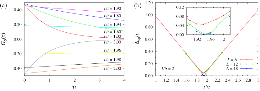
Next let us consider the interacting case with the Hamiltonian , where , and . In Fig. 13(a), the imaginary time dependence of the off-diagonal component of the Green’s function at the point is shown. The area under corresponds to the coefficients [cf. Eqs. (32) and (33)], hence a change in the topological invariant can be related to sign change of the area under . As can be seen in Fig. 13(a), for and , this change occurs between and , and correspondingly, the invariant jumps from to . This means the topological-to-trivial band insulator transition occurs at a value of – smaller than in the noninteracting case, where the critical values is . This can be understood as the consequence of the super-exchange induced by the Coulomb repulsion which favors the singlet formation on the -bonds. Similar to the GKM-Hubbard model, the topological transition in DKM-Hubbard model is also associated with the closing of the single-particle gap at , which may be obtained from the decay in imaginary time of the diagonal Green function and is shown in Fig. 13(b). The gap closes at and thus supports the fact that the invariant correctly captures the interaction effects which lead to destabilize the topological phase with respect to the noninteracting case.
3.2.3 Limitations of the Invariant in QMC simulations
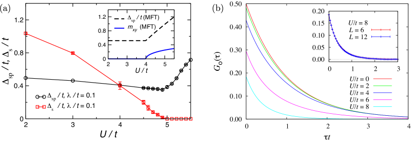
In the case, where the onsite Coulomb repulsion is large enough, previous studies[25, 26, 27] have shown that the system enters a transverse antiferromagnetically ordered Mott-insulating phase. With the onset of magnetic order, the time-reversal symmetry is spontaneously broken. The phase transition from topological insulator to the antiferromagnetically ordered phase at a fixed value of by increasing , is however, not accompanied by the closing of the single-particle gap. As shown in Fig. 14(a) for the KMH model at and as a function of , the single-particle gap merely exhibits a cusp at the transition point, . Since the antiferromagnetically ordered Mott-insulating phase breaks the SU(2) spin rotational symmetry and Goldstone modes emerge in the thermodynamic limit, it is actually the spin gap, defined from dynamic spin-spin correlation function, , that closes at the transition point, . This transition from the topological insulator to the antiferromagnetical Mott insulator is induced by collective excitations at the two-particle level. The topological invariant based on the zero-frequency Green can only capture physics in the single-particle sector, and hence fails to detect this transition. This can also be seen in Fig. 14(b), for the KMH model, where is shown for different values fo at .[42] The magnetic transition happens near , however the off-diagonal component of the Green’s function exhibits no qualitative change for increasing interactions.
In contrast to the sign change of as one scan acrossing the topological phase transition shown in Fig. 13(a), in Fig. 14(b) remains positive as the interaction strength varies across the topological insulator to antiferromagnetic Mott insualtor transition point. We emphasize that this does not appear to be a mere finite size effect, as can be seen in the inset of Fig. 14(b), where we compare the QMC data at for two different system sizes, and , and fall perfectly on top of each other. The results are seen to indeed be converged in the finite sizes we have studied. The associated proportionality coefficients which correspond to the area under are shown in Fig. 15 as a function of and verify the issue. Figure 15(a) shows that, although the values of decay near the expected , there is no sign change in upon tuning through the critical value for all values of we have studied. Fig. 15(b) considers finite size dependence of versus at . Again, the absence of strong finite size effects is obvious.
Both, Fig. 14 and Fig. 15 suggest that the invariant stays constant across the topological insulator to antiferromagnetic Mott insulator phase transition. Once the system enters the antiferromagnetic ordered phase, the time-reversal and inversion- (sublattice) symmetries of the Hamiltonian are spontaneously broken. This happens at the two-particle level and hence cannot be monitored by the single-particle Green’s function, on which the calculation of the invariant is based. Strictly speaking, the spontaneous breaking of spin- and time-reversal-symmetry applies only to the thermodynamic limit. While order parameters can acquire finite values on finite size lattices, no symmetry, neither continuous nor discrete, can be spontaneously broken unless in the thermodynamic limit. Hence the invariant formalism Eq. (36) is formally well defined on finite-size lattices. While spontaneous symmetry breaking in the ordered phase implies a degenerate ground state subspace in the limit of infinite system size, in finite-size simulation the ground state is given by the linear combination of equal weight of states from this manifold. In our case all the different spin-orientated symmetry breaking states have equal weight, such that measurements on this ground state are not able to distinguish any preferred magnetic ordering.
Even if the interaction strength is large enough to trigger spontaneous symmetry breaking in the thermodynamic limit, our results in Figs. 14 and 15 do not indicate any qualitative change with increasing system size. Thus, limited to the single-particle sector, the topological invariant is still blind with respect to collective excitations and the associated spontaneous symmetry breaking. Its usage as a reliable indicator of the topological nature of phases (or lack thereof) should therefore be restricted to cases where the transition from the topological insulator to the topological trivial phase is also indicated by the closing of the single-particle gap. In this regard, it does not really matter whether the vanishing of the single-particle excitation gap at the critical point is due to the underlying physics, or the artifacts associated with the method used. Indeed, the successful application of the topological invariant has been shown in, e.g., correlated electron systems in one dimension using the numerically exact time-dependent density matrix renormalization group (DMRG) approach;[71] For two-dimensional interacting systems in the approximative approaches using mean-field theory[20] and the variational cluster approximation (VCA)[72] applied to the KMH model; Dynamical mean-field theory (DMFT) has been employed to study the interaction-driven transition between topological states in a Kondo insulator[73] and cluster DMFT to study model for three-dimensional correlated complex oxides, the pyrochlore iridates.[74] In these cases the topological invariant still allows for highly accurate determination of the critical point. Recently, topological invariants expressed in terms of ground state wavefunction are proposed for topological insulators,[75] which are valid in the presence of arbitrary interaction. From the current numerical perspective, the Green’s function remains the most efficient approach within the realm of its validity.
3.3 The Spin Chern Number
In addition to the invariant, the topological insulators can also be characterized by the spin Chern number (cf. Sec. 2.1), that is the Chern number for one spin flavor. It has been shown that without the Rashba coupling, the spin Chern number is still a good indicator for the QSH state.[49, 50] On one hand, the Chern number can be obtained from a many-body wave function with twisted boundary conditions.[70] On the other hand, the spin Chern number can be evaluated in terms of the projection operators as[4]
| (41) | |||||
where is the spectral projector operator constructed using the Bloch eigenvectors at with energies below the Fermi energy , i.e., . Although the formalism was first proposed for noninteracting systems, we can also compute the interacting spin Chern number with the QMC method. In an analogy with the invariant, the Bloch eigenstates are replaced with the R-zero eigenvectors of the zero-frequency Green’s functions , and then
| (42) |
where choosing corresponds to selecting occupied bands , i.e. R-zero of the . In finite-size systems, the integration over the Brillouin zone is substituted by summation of discrete momentum points. For a lattice grid with spacing , we can approximate the and as
| (43) |
Thus, the spin Chern number in Eq. (41) can be approximated as[39]
| (44) | |||||
Under such a construction, the evaluation of the spin Chern number in the QMC simulations might look like subject to strong finite-size effect and an quantized value of it is not guaranteed. However, we will demonstrate that, although subject to finite size effects, a jump in can be clearly observed across the topological phase transition. This suggests that the spin Chern number is a reliable means to detect topological properties even in the interacting systems.
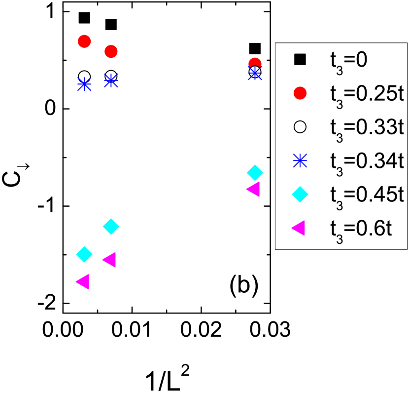
As an example we compute the spin Chern number in the GKM model with interactions.[39] Figure 16(a) shows the comparison of the invariant and the spin Chern number in the GKM-Hubbard model at as a function of . Although the spin Chern number is poorly quantized, in particular as is approaching to the transition (where increasingly more Monte Carlo samples are needed to recover the time-reversal symmetric relation within statistical errors), a jump in can be clearly seen.
This suggests that the spin Chern number is also reliable to detect the topological phase transition at the interacting level. Moreover, the poor quantization in the spin Chern number is attributed to strong finite-size effects. The expected quantized value can still be identified upon approaching to larger system sizes. As an example, a tentative finite-size analysis of the spin Chern number is shown in Fig. 16(b). Away from the topological phase transition, the quantized spin Chern number behavior can still be captured in the thermodynamic limit. One can see that in the small regime, whereas in the large limit, . Thus we can still distinguish the discrepancy during the topological phase transition at the interacting level. For details we refer the reader to Ref. \refciteHung2013b. Note, that based on the single-particle Green’s function, the use of the spin Chern numbers to characterize the topological nature of a phase underlies the same limitations as the invariant discussed in Sec. 3.2.3. The major advantage over the topological invariant, evaluated at the TRIM, is that the spin Chern number can be even applied in systems without inversion symmetry.
4 Conclusion and Outlook
The main objective of this review is to show how to detect the topological nature of the KM model in the presence of electron correlations within QMC simulations. To this end, we discuss three specific approaches and their application within the determinant quantum Monte Carlo technique, with which the KMH model can be studied in a unbiased manner. One special merit of the half-filled KMH model is that the time-reversal symmetry and the particle-hole symmetry allow for simulations free of the minus-sign problem – hence the interplay of the topological properties of the system with electronic interactions can be studied numerically exact.
The first approach is the idea of characterizing the topological phase transition with magnetic flux insertion. We showed that the invariant can quantify the fluxon induction ( pumping) due to pairs of fluxes threaded through plaquettes of the system.
Next we explained in detail the idea of evaluating the invariant in terms of zero frequency Green’s function. Due to the inversion symmetry in the KMH systems, one only needs to evaluate the parity of the eigenstates of the zero-frequency Green’s function at the time-reversal invariant momenta. We provide two examples models, the generalized KMH model and dimerized KMH model, and show that in the interacting case the formulation of the index evaluation can be easily calculated from zero-frequency Green’s functions. Both models indicate a topological phase transition upon varying tight-binding parameters. We show that the correlation effects stabilize the order in the generalized KMH model, but destabilize it in the dimerized KMH model. Although the invariant could be used to successfully within QMC simulations for the KMH model systems, it is subject to limitations. We discuss the quantum phase transition from topological insulator to the magnetic insulator, which occurs at the two-particle level, i.e., susceptibilities diverge, and where the zero frequency single-particle Green’s function is not able to capture such transitions. New ideas and formalisms are needed in these situations.
The third approach, accessible to detect topological phase transitions within QMC simulations, is to directly measure the spin Chern number. Although under strong finite-size effects, the spin Chern number measurement proves to present another useful topological quantity in correlated topological insulators and can be even applied in systems intrinsically without inversion symmetry.
The three approaches above have their individual benefits and limitations, but allow us to gather unbiased information on the topological nature in the correlated quantum spin Hall system from simulations. Besides the KMH model, topological phase transitions can be realized in more general models and systems, which do not retain particle-hole, inversion-, or even the time-reversal symmetry. In realistic condensed matter materials, which might host topological states (topological insulator, axion insulator, topological Mott insulator, or topological supercoductor),[76] electron correlations and strong spin-orbit coupling are competing in a multi-orbital environment (such as the electron iridates compounds). Here the plain Hubbard model is not sufficient to capture the physics and more advanced model such as the Kanamori-type Hamiltonian would be the starting point.[77] In these situations, more versatile numerical techniques are needed – the hybridization expansion continuous-time QMC cluster dynamical mean field framework is a promising example among several others. But just as the presented QMC studies of the KMH model in this review, a combination of accurate, controlled numerical techniques and clear theoretical understanding can indeed facilitate controlled investigations of novel physics in correlated topological systems.
Acknowledgments
We thank Fakher Assaad, Victor Chua, Xi Dai, Andrew Essin, Gregory Fiete, Zheng-Cheng Gu, Victor Gurarie, Martin Hohenadler, Alejandro Muramatsu, Lei Wang, Zhong Wang and Stefan Wessel for collaboration and discussions. HHH and ZYM are grateful for the hospitality from Institute for Advanced Study, Tsinghua University and Institute of Physics, Chinese Academy of Sciences. ZYM acknowledges the supported by the NSERC, CIFAR, and Centre for Quantum Materials at the University of Toronto. HHH acknowledges the support by Grant No. ARO W911NF-09-1-0527, Grant No. NSF DMR-0955778, Grant No. ARO W911NF-12-1-0573 with funding from the DARPA OLE Program and computer time at Texas Advanced Computing Center at the University of Texas, Austin and the Brutus cluster at ETH Zürich. TCL acknowledges JARA-HPC and JSC Jülich for the allocation of CPU time.
References
- [1] K. v. Klitzing, G. Dorda, and M. Pepper, Phys. Rev. Lett. 45 (1980) 494.
- [2] B. I. Halperin, Phys. Rev. B 25 (1982) 2185.
- [3] D. J. Thouless, M. Kohmoto, M. P. Nightingale, and M. den Nijs, Phys. Rev. Lett. 49 (1982) 405.
- [4] J. E. Avron, R. Seiler, and B. Simon, Phys. Rev. Lett. 51 (1983) 51.
- [5] X.-G. Wen, arXiv:1301.7675.
- [6] C. L. Kane and E. J. Mele, Phys. Rev. Lett. 95 (2005) 146802.
- [7] C. L. Kane and E. J. Mele, Phys. Rev. Lett. 95 (2005) 226801.
- [8] X. C. Xu and J. E. Moore, Phys. Rev. B 73 (2006) 045322.
- [9] X.-L. Qi, Y.-S. Wu, and S.-C. Zhang, Phys. Rev. B 74 (2006) 085308.
- [10] B. A. Bernevig, T. L. Hughes, and S.-C. Zhang, Science 314 (2006) 1757.
- [11] M. König, S. Wiedmann, C. Brüne, A. Roth, H. Buhmann, L. W. Molenkamp, X.-L. Qi, and S.-C. Zhang, Science 318 (2007) 766.
- [12] L. Fu and C. L. Kane, Phys. Rev. B 76 (2007) 045302.
- [13] L. Fu, C. L. Kane, and E. J. Mele, Phys. Rev. Lett. 98 (2007) 106803.
- [14] H. J. Zhang, L. C. Xing, X.-L. Qi, X. Dai, F. Zhong, S.-C. Zhang, Nature Physics 5 (2009) 438.
- [15] Y. L. Chen, J. G. Analytis, J.-H. Chu, Z. K. Liu, S.-K. Mo, X.-L. Qi, H. J. Zhang, D. H. Lu, X. Dai, Z. Fang, S. C. Zhang, I. R. Fisher, Z. Hussain, Z.-X. Shen, Science 325 (2009) 178.
- [16] B. Roy and I. F. Herbut, Phys. Rev. B 88 (2013) 045425.
- [17] M. König, H. Buhmann, L. W. Molenkamp, T. Hughes, C.-X. Liu, X.-L. Qi, and S.-C. Zhang, J. Phys. Soc. Jpn. 77 (2008) 031007.
- [18] J. Maciejko, T. L. Hughes, and S.-C. Zhang, Annu. Rev. Condens. Matter Phys. 2 (2011) 31.
- [19] C. Wu, B. A. Bernevig, and S.-C. Zhang, Phys. Rev. Lett. 96 (2006) 106401.
- [20] S. Rachel and K. Le Hur, Phys. Rev. B 82 (2010) 075106.
- [21] A. Vaezi, M. Mashkoori, and M. Hosseini, Phys. Rev. B 85 (2012) 195126.
- [22] Y. Yamaji and M. Imada , Phys. Rev. B 83 (2011) 205122.
- [23] W. Wu, S. Rachel, W.-M. Liu, and K. Le Hur, Phys. Rev. B 85 (2012) 205102.
- [24] S.-L. Yu, X. C. Xie, and J.-X. Li, Phys. Rev. Lett. 107 (2011) 010401.
- [25] M. Hohenadler, T. C. Lang, and F. F. Assaad, Phys. Rev. Lett. 106 (2011) 100403.
- [26] D. Zheng, G. M. Zhang, and C. Wu, Phys. Rev. B 84 (2011) 205121.
- [27] M. Hohenadler, Z. Y. Meng, T. C. Lang, S. Wessel, A. Muramatsu, and F. F. Assaad, Phys. Rev. B 85 (2012) 115132.
- [28] J. E. Moore. Nature 452 (2008) 970.
- [29] M. Z. Hasan and C. L. Kane, Rev. Mod. Phys. 82 (2010) 3045.
- [30] X.-L. Qi and S.-C. Zhang, Physics Today 63 (2010) 33.
- [31] X.-L. Qi and S.-C. Zhang, Rev. Mod. Phys. 83 (2011) 1057.
- [32] M. Z. Hasan and J. E. Moore, Annu. Rev. Condens. Matter Phys. 2 (2011) 55.
- [33] G. A. Fiete, V. Chua, M. Kargarian, R. Lundgren, A. Rüegg, J. Wen, and V. Zyuzin Physica E 44 (2012) 845.
- [34] M. Hohenadler and F. F. Assaad, J. Phys.: Condens. Matter 25 (2013) 143201.
- [35] H. Weng, Xi Dai, and Zhong Fang, Asia Pac. Phys. Newslett. 1 (2012) 31.
- [36] Y. Ando, J. Phys. Soc. Jpn. 82 (2013) 102001.
- [37] F. F. Assaad, M. Bercx, and M. Hohenadler, Phys. Rev. X 3 (2013) 011015.
- [38] L. Fu and C. L. Kane, Phys. Rev. B 74 (2006) 195312.
- [39] H.-H. Hung, V. Chua, L. Wang, and G. A. Fiete, arXiv:1307.2659.
- [40] Z. Wang and S.-C. Zhang, Phys. Rev. X 2 (2012) 031008.
- [41] H.-H. Hung, L. Wang, Z.-C. Gu and G. A. Fiete, Phys. Rev. B 87 (2013) 121113(R).
- [42] T. C. Lang, A. M. Essin, V. Gurarie, and S. Wessel, Phys. Rev. B 87 (2013) 205101.
- [43] F. D. M. Haldane, Phys. Rev. Lett. 61 (1988) 2015.
- [44] A. H. Castro Neto, F. Guinea, N. M. R. Peres, K. S. Novoselov, and A. K. Geim, Rev. Mod. Phys. 81 (2009) 109.
- [45] C. L. Kane, Int. J. Mod. Phys. B 21 (2007) 1155.
- [46] M. Ezawa, Y. Tanaka, and N. Nagaosa, arXiv:1307.7347.
- [47] Y. Yang, H. Li, L. Sheng, R. Shen, D. N. Sheng, and D. Y. Xing, arXiv:1301.1618.
- [48] S. Rachel, arXiv:1310.3159.
- [49] L. Sheng, D. N. Sheng, C. S. Ting, and F. D. M. Haldane, Phys. Rev. Lett. 95 (2005) 136602.
- [50] D. N. Sheng, Z. Y. Weng, L. Sheng, and F. D. M. Haldane, Phys. Rev. Lett. 97 (2006) 036808.
- [51] F. Goth, D. J. Luitz, F. F. Assaad, Phys. Rev. B 88 (2013) 075110.
- [52] F. F. Assaad, NIC Series Vol. 10 (2002).
- [53] F. F. Assaad and H. G. Evertz, Lect. Notes Phys. 739 (2008) 277.
- [54] G. Sugiyama, S. E. Koonin, Ann. Phys. 168 (1986) 1.
- [55] S. Sorella, S. Baroni, R. Car, and M. Parrienllo, Europhys. Lett. 8 (1989) 663.
- [56] S. R. White, D. J. Scalapino, R. L. Sugar, E. Y. Loh, and J. E. Gubernatis, Phys. Rev. B 40 (1989) 506.
- [57] Z. Y. Meng, T. C. Lang, S. Wessel, F. F. Assaad, and A. Muramatsu, Nature 464 (2010) 847.
- [58] S. Sorella, Y. Otsuka, and S. Yunoki, Sci. Rep. 2 (2012) 992.
- [59] F. F. Assaad and M. Imada, J. Phys. Soc. Jpn. 65 (1996) 189.
- [60] M. Feldbacher and F. F. Assaad, Phys. Rev. B 63 (2001) 073105.
- [61] F. F. Assaad and I. F. Herbut, Phys. Rev. X 3 (2013) 031010.
- [62] Z. Wang, X.-L. Qi, and S.-C. Zhang, Phys. Rev. B 85 (2012) 165126.
- [63] Y. Ran, A. Vishwanath, and D.-H. Lee, Phys. Rev. Lett. 101 (2008) 086801.
- [64] X.-L. Qi and S.-C. Zhang, Phys. Rev. Lett. 101 (2008) 086802.
- [65] Z. Wang, X.-L. Qi, and S.-C. Zhang, Phys. Rev. Lett. 105 (2010) 256803.
- [66] X.-L. Qi, T. L. Hughes, and S.-C. Zhang, Phys. Rev. B 78 (2008) 195424.
- [67] Z. Wang and S.-C. Zhang, Phys. Rev. B 86 (2012) 165116.
- [68] Z. Wang and B. Yan, J. Phys.: Condens. Matter 25 (2013) 155601.
- [69] V. Gurarie, Phys. Rev. B 83 (2011) 085426.
- [70] Q. Niu, D. J. Thouless, and Y.-S. Wu, Phys. Rev. B 31 (1985) 3372.
- [71] S. R. Manmana, A. M. Essin, R. M. Noack, and V. Gurarie, Phys. Rev. B 86 (2012) 205119.
- [72] J. C. Budich, R. Thomale, G. Li, M. Laubach, and S.-C. Zhang, Phys. Rev. B 86 (2012) 201407.
- [73] J. Werner, F. F. Assaad, Phys. Rev. B 88 (2013) 035113.
- [74] A. Go, W. Witczak-Krempa, G. S. Jeon, K. Park, and Y. B. Kim, Phys. Rev. Lett. 109 (2012) 066401.
- [75] Z. Wang and S. C. Zhang, arXiv:1308.4900.
- [76] W. Witczak-Krempa, G. Chen, Y. B. Kim, L. Balents, arXiv:1305.2193.
- [77] C. M. Puetter, H. Y. Kee, Europhys. Lett. 98 (2012) 27010.