Cosmological Constraints on Bose-Einstein-Condensed Scalar Field Dark Matter
Abstract
Despite the great successes of the Cold Dark Matter (CDM) model in explaining a wide range of observations of the global evolution and the formation of galaxies and large-scale structure in the Universe, the origin and microscopic nature of dark matter is still unknown. The most common form of CDM considered to-date is that of Weakly Interacting Massive Particles (WIMPs), but, so far, attempts to detect WIMPs directly or indirectly have not yet succeeded, and the allowed range of particle parameters has been significantly restricted. Some of the cosmological predictions for this kind of CDM are even in apparent conflict with observations (e.g. cuspy-cored halos and an overabundance of satellite dwarf galaxies). For these reasons, it is important to consider the consequences of different forms of CDM. We focus here on the hypothesis that the dark matter is comprised, instead, of ultralight bosons that form a Bose-Einstein Condensate, described by a complex scalar field, for which particle number per unit comoving volume is conserved. We start from the Klein-Gordon and Einstein field equations to describe the evolution of the Friedmann-Robertson-Walker universe in the presence of this kind of dark matter. We find that, in addition to the radiation-, matter-, and -dominated phases familiar from the standard CDM model, there is an earlier phase of scalar-field-domination, which is special to this model. In addition, while WIMP CDM is non-relativistic at all times after it decouples, the equation of state of Bose-Einistein condensed scalar field dark matter (SFDM) is found to be relativistic at early times, evolving from stiff () to radiationlike (), before it becomes non-relativistic and CDM-like at late times (). The timing of the transitions between these phases and regimes is shown to yield fundamental constraints on the SFDM model parameters, particle mass and self-interaction coupling strength . We show that SFDM is compatible with observations of the evolving background universe, by deriving the range of particle parameters required to match observations of the cosmic microwave background (CMB) and the abundances of the light elements produced by big bang nucleosynthesis (BBN), including , the effective number of neutrino species, and the epoch of matter-radiation equality . This yields eV and . Indeed, our model can accommodate current observations in which is higher at the BBN epoch than at , probed by the CMB, which is otherwise unexplained by the standard CDM model involving WIMPs. We also show that SFDM without self-interaction (also called “fuzzy dark matter”) is not able to comply with the current constraints from BBN within 68% confidence, and is therefore disfavored.
- PACS numbers
-
98.80.-k, 95.35.+d, 98.80.Cq, 98.80.Ft
pacs:
98.80.-k, 95.35.+d, 98.80.Cq, 98.80.FtI Introduction
I.1 Cold dark matter
Since the discovery of the accelerating expanding Universe, has become the standard cosmological model as supported by various astronomical observations. Cosmic microwave background (CMB) observations have shown that about 25% of the energy density of the present Universe is comprised of non-baryonic cold dark matter. Cold dark matter (CDM) does not interact under electromagnetism and the strong force, and moves non-relativistically, thus acting like cold, pressureless dust in the present Universe. Despite these characteristics, its particle nature is still unknown and no candidate can be found within the Standard Model of particle physics (SM). So far, diverse extensions of the SM have predicted candidate particles for CDM, among which the most popular ones at present are in the form of weakly interacting massive particles (WIMPs) (see Refs. GW1985; ST1986; DFS1986). WIMPs are collisionless and massive ( GeV).
The standard collisionless CDM, in a universe perturbed by Gaussian-random-noise primordial density fluctuations with a nearly scale-independent primordial power spectrum, provides a well-accepted scenario for cosmic structure formation: the hierarchical clustering of dark matter fluctuations and the infall of baryons into CDM potential wells after recombination, to form galaxies. Despite the fact that this story line is in good agreement with many observational constraints, including CMB anisotropy EWMAP7; WMAP9; Planck, large-scale structure BAOBOSS9; 2PCFBOSS9 and the general properties of dark-matter-dominated halos Walker2009; Newman2013; Vikhlinin2009, some crucial issues on small scales are subject to controversy (see Ref. WD2013CDMP for a recent, brief review). First, hierarchical clustering in the standard CDM model overpredicts the number of substructures in a halo the size of the Local Group by an order of magnitude as compared with the number of satellite galaxies observed in the Local Group, a discrepancy referred to as the “missing satellite problem” (see Refs. Klypin1999; Moore2; Aquarius2008; MSII2009). Second, the density profiles of collisionless CDM halos in N-body simulations show a universal profile with a central cusp ( in the NFW profile NFW), while observations of low-surface brightness galaxies and dwarf galaxies mostly favor a flat central slope. This has been known as the “cuspy core problem” (see Refs. Moore1; dB2001; Oh2008; Amorisco2012). Furthermore, current dark matter detection experiments, both direct and indirect ones, have not yet discovered any compelling signals of WIMPs Bauer2013DMDETECT. As a matter of fact, while WIMPs are mostly expected to be the lightest supersymmetric particle in the Minimal Supersymmetric Standard Model (MSSM), e.g., neutralinos GK2000, recent data from the Large Hadron Collider has found no evidence of a deviation from the SM on GeV scales, significantly restricting the allowed region of MSSM parameters ATLAS2013; CMS2013. All these facts taken together, it is evident that the microscopic nature of dark matter is sufficiently unsettled as to justify the consideration of alternative candidates for the CDM paradigm, especially in the hope of resolving the above difficulties.
I.2 Bose-Einstein-condensed ultra-light particles as dark matter candidate
We assume that the dark matter particles are described by a spin-0 scalar field (‘scalar field dark matter’, for short; henceforth, SFDM) with a possible self-interaction. In fact, one type of bosonic particle suggested as a major candidate for dark matter is the QCD axion. It is the pseudo-Nambu-Goldstone boson in the Peccei-Quinn mechanism, proposed as a dynamical solution to the strong CP-problem in QCD. For the axion to be CDM, it has to be very light, eV Weinberg; Sikivie2012.
In addition to the QCD axion, several fundamental scalar fields have been predicted by a variety of unification theories, e.g., string theories and other multi-dimensional theories Carroll1998; ADD1999; Kallosh2002; Arvanitaki2010. The bosonic particles envisaged are typically ultralight, with masses down to the order of eV. This suggests an ultrahigh phase-space density, leading to the possibility of formation of a Bose-Einstein condensate (BEC), i.e., a macroscopic occupancy of the many-body ground state. In principle, for a fixed number of (locally) thermalized identical bosons, a BEC will form if , where is the number density and is the de Broglie wavelength. This is equivalent to there being a critical temperature , below which a BEC can form.
For a non-relativistic, ideal (i.e. non-interacting) boson gas, the well-known result for is
| (1) |
which was used, for example, by Refs. Harko2011; FM2009. Equation (1) is not an adequate description of the case considered here, however. For the ultralight particles with which we are concerned, , so a fully relativistic treatment is required.
We are interested in a complex scalar field, for which the presence of dark matter results from the asymmetry associated with the difference between the number density of bosons and that of their anti-particles, a conserved charge density in the comoving frame (see also Appendix LABEL:app:charge for more discussion about the charge). A fully relativistic treatment of Bose-Einstein (‘BE’) condensation was given by Refs. Kapusta1981 and HW1982, including the relationship between BE condensation and symmetry breaking of a scalar field. Those authors showed that, for an ultra-relativistic ideal charged boson gas, described by a complex scalar field,
| (2) |
where is the charge per unit proper volume. This does not, however, take self-interaction into account. Reference HW1982 showed that, in the case of an adiabatically expanding boson gas, relevant to cosmology, if the scalar field has a generic quartic self-interaction, then the bosons must either be condensed at all temperatures (i.e. at all times) or else never form a BEC. In this case, the charge per unit comoving volume, , and entropy per unit comoving volume, , are both conserved. According to equation (4.7) of that paper, a (local) BEC will exist from the beginning and remain at all times, if
| (3) |
where is the dimensionless coupling strength of the quartic self-interaction, in natural units. Our SFDM has essentially zero entropy per unit comoving volume. Also, for the small boson masses that we will be considering, the conserved charge density in the comoving frame, , is extremely high, given the observed present-day dark matter energy density , for . Therefore, we are always in the regime described by inequality (3), and thus the bosons are fully condensed from the time they are born, i.e., almost all of the bosons occupy the lowest available energy state.
Hence, the cosmological Bose-Einstein-condensed SFDM can be described by a single (coherent) classical scalar field, of which the value at each point in space equals to that of the local order parameter Pitaevskii. Even though the condensation requires Bose-Einstein statistics in the first place, i.e., local thermalization (see Refs. SY2009; Erken2012), we argue that thermal decoupling within the bosonic dark matter can occur when the expansion rate exceeds its thermalization rate, without disturbing the condensate. Most of the bosons will stay in the ground state (BEC), and the classical field (SFDM) remains a good description, analogous to the fact that CMB photons after decoupling still follow a black-body distribution. In summary, we consider the Bose-Einstein condensate as an initial condition for our model, such that we can use and trust the effective field description throughout the evolution of the universe up to very early times.
A scalar field description of BEC dark matter has been studied by several authors before; see, for instance, Refs. Sin; LeeKoh; Goodman; HBG; Harko2011; Magana2012; RS1; Chavanis2012. With regard to the aforementioned initial condition, one may also envisage a scenario in which the coherent scalar field is created gravitationally at the end of inflation, as has been considered, e.g., by Refs. Ford; PV1999Q; Peebles2000. On the other hand, it might also be that SFDM was just another scalar field, in place along with the inflaton before and during inflation FHW1992; ALS2002, emanating from yet earlier initial conditions. Speculations of that kind are beyond the scope of this paper. However, we find some interesting early-time features which will deserve more discussion in due course.
A prime motivation for studying SFDM has been its ability to suppress small-scale clustering and hence potentially resolve the dark matter problems mentioned above. For non-self-interacting particles, sets a natural lower limit to the scale on which equilibrium halos can form, where corresponds to the virial velocity of the galactic halos. While this paper shall deal only with the consequences of SFDM for the homogeneous background universe, this argument would suggest that there is a lower limit to the particle mass for SFDM of eV, since then kpc RS1; RS2, the core size of the dark matter halo of a typical dwarf spheroidal galaxy in the present Universe Amorisco2013. If self-interaction of SFDM is included, the associated characteristic gravitational equilibrium scale is proportional to , where is the dimensional coupling strength of the quartic self-interaction (related to by , i.e., kpc if eV-1 cm3, and for this ratio of , eV cm3 when eV (see Refs. RS1, and references therein). Therefore, SFDM provides and as two mechanisms to suppress small-scale structures. When , only is responsible for affecting structure formation. This is the self-interaction-dominated limit, also known as the Thomas-Fermi regime; we called it TYPE II BEC-CDM in Ref. RS1. We will also address the limit in which there is no self-interaction (i.e. , also known as fuzzy dark matter (FDM) in Refs. HBG; WC2009; we called it TYPE I BEC-CDM in Ref. RS1).
This paper is organized as follows: in Section II, we present the fundamental equations underlying the description of SFDM with a quartic, positive self-interaction. In Section III, we solve for the homogenous background evolution of a universe with the same cosmic inventory as CDM, but with CDM replaced by SFDM, over cosmic time. We identify three distinctive phases in the evolution of SFDM: non-relativistic, dust-like behavior at late times, which is indicative of the usefulness of SFDM as cold dark matter, a radiationlike phase at intermediate times, and an even earlier phase when SFDM behaves as a “stiff” relativistic fluid. We note that SFDM is relativistic in both the radiationlike phase and the stiff phase (in this work, the word “relativistic” does not only refer to radiation, but generally refers to any type of matter for which the ratio of pressure to energy density is in the physically allowed range ). While the former two phases and the corresponding constraint from the time of matter-radiation equality at have been identified and appreciated previously (e.g. in Refs. Goodman; Peebles2000), the latter one has only been sporadically encountered, and often as a result of special assumptions; see, e.g. Refs. Joyce1997; ALS2002; Dutta2010. However, we find that the stiff phase is generic for complex SFDM, no matter which values of SFDM parameter one adopts. We will comment more on this later. In Section IV, we present the most important results of this work, namely the constraints on the SFDM model parameters, boson mass , and positive boson self-interaction coupling strength (or equivalently , in which the final results will actually be presented), which follow from the constraints on the homogeneous background evolution by current cosmological observations. These include the aforementioned redshift of matter-radiation equality and the effective number of neutrino species at the time of big bang nucleosynthesis (BBN). They constrain the timing and longevity of the stiff and radiationlike phases of SFDM, and thereby set severe restrictions on the allowed parameter space. Finally, Section V contains detailed discussions on the many implications of our results, while Section VI presents a brief summary. Appendices A-LABEL:app:matching contains some more technical aspects which have been deferred from the main text, but help to make the presentation more self-contained.
In deriving those constraints on SFDM in concordance with current cosmological observations, we obtain three main results: First, we are able to restrict the allowed parameter space of SFDM severely, despite the fact that we limit our consideration to the homogeneous background universe. Second, there, nevertheless, remains a semi-infinite stripe in parameter space which is in accordance with observations, including parameter sets which are able to resolve the small-scale problems of CDM. Third, the currently favored value of during BBN, which exceeds the standard value of 3.046 for a universe containing just three neutrino species and no extra relativistic species, excludes the possibility that the dark matter is SFDM with vanishing self-interaction, i.e., fuzzy dark matter, at confidence. On the contrary, SFDM with self-interaction provides a natural explanation of why during BBN Steigman2012 is higher than that inferred from the Cosmic Microwave Background Planck.
II Basic equations
We will assume in this paper that dark matter is described by a complex field. There are several motivations for considering a complex, rather than a real field, namely the U(1) symmetry corresponding to the dark matter particle number (charge) conservation (see Appendix LABEL:app:charge and Ref. BCK2002), and the richer dynamics of halos, e.g. formation of vortices (see Refs. RS1; RS2).
II.1 Equation of motion for SFDM
The ground state of a bosonic system can be described by a classic scalar field theory. We choose the following generic Lagrangian density of the complex scalar field
| (4) |
The metric signature we adopt here is . The potential in the Lagrangian above contains a quadratic term accounting for the rest-mass plus a quartic term accounting for the self-interaction
| (5) |
This model has been adopted in other works, as well; see, e.g., Refs. Goodman, PV1999, MM2012. We choose physical units throughout, in contrast to the convention usually used in high-energy particle physics. The main reason is that this is the first paper in a series of works on the cosmological behavior of SFDM, which will include the linear and nonlinear growth of fluctuations. There, we are concerned with non-relativistic () and classical limits (), where natural units become disadvantageous. In order for to have units of energy density, the field has units of and the unit for the coupling constant is eV cm3. A value of eV cm3 would correspond to . For the purpose of comparison, we take a look at the dimensionless self-interaction strength of QCD axions. According to equation (2) and (3) in Ref. SY2009, , also tiny, for the axion decay constant GeV.
The quartic term in the above potential models the two-particle self-interaction. It is a good approximation to ignore higher order interactions when the bosonic gas is dilute, i.e., when the particle self-interaction range is much smaller than the mean interparticle distance. Moreover, since particles in non-zero-momentum states can be neglected, it is sufficient to consider only two-body s-wave scatterings. This means the coupling coefficient is a constant and related to the s-wave scattering length as , which is effectively the first Born approximation.
The equation of motion for the scalar field is the relativistic Klein-Gordon equation,
| (6) |
or
| (7) |
where is the metric tensor and is the Christoffel symbol, calculated in Appendix A.1 for the perturbed Friedmann-Robertson-Walker (FRW) metric. Combining such a metric in the conformal Newtonian gauge with the Klein-Gordon equation (7) yields
| (8) |
Here, denotes the scale factor of the expanding FRW universe, and and are the perturbations to the otherwise homogeneous metric (see Appendix A, where we summarize some of the more technical, but otherwise known derivations).
II.2 Einstein field equations
The perturbed metric given by equation (35) is related to the total mass-energy density of the universe through the Einstein field equations. With the Ricci tensor calculated in Appendix A.3, let us consider the contribution from the time-time component,
| (9) |
In fact, the left-hand side is
{IEEEeqnarray}rCl
R^0_ 0-12R & = (1-2Ψ/c^2)R_00-R/2
= 3(da/dt)2c2a2+2∇2Φc2a2-
-6da/dtc4a(∂_tΦ+da/dtaΨ).
Thus, the time-time component (9) becomes
| (10) |
We can evaluate the contribution of the scalar field to the energy-momentum
tensor, using the Lagrangian density in equation (4) and
equation (41), which yields
{IEEEeqnarray}rCl
T_μν, SFDM & = ℏ22m(∂_μψ^*∂_νψ+∂_νψ^*∂_μψ)-
-g_μν(ℏ22mg^ρσ∂_ρψ^*∂_σψ-
-12mc^2—ψ—^2-λ2—ψ—^4).
Its time-time component is recognized as
{IEEEeqnarray}rCl
T^0_ 0, SFDM & = H=ℏ22mc2(1-2Ψc2)—∂_tψ—^2+
+ ℏ22ma2(1+2Φc2)—∇ψ—^2+
+ 12mc^2—ψ—^2+12λ—ψ—^4.
where is the Hamiltonian density of SFDM. Note
that is not invariant under coordinate
transformations, because matter is coupled to the gravitational
field, hence the energy of the bosons is not conserved.
III Homogenous background universe
III.1 Mass-energy content of the FRW universe and the Friedmann equation
In this paper, we will consider a universe with the same cosmic inventory as the basic CDM model except that CDM is replaced by SFDM (we will call it SFDM model from now on). We will use the set of cosmological parameters from the recent Planck data release Planck (listed as basic in Table 1) to solve for the evolution of the homogeneous background universe below. From those we derive some other cosmological parameters needed for the calculation. Note again that here refers to the present-day SFDM energy density instead of CDM. We will see later that SFDM indeed behaves as CDM at present. accounts for the ordinary radiation component, i.e., photons and the Standard Model neutrinos. For simplicity, the neutrinos are considered as massless so that the total matter density fraction today is , where stands for the baryon density fraction at present. The density fraction of the cosmological constant is .
| Basic | Derived | ||
|---|---|---|---|
| 0.673 | 0.14187 | ||
| 0.02207 | |||
| 0.1198 | 3390 | ||
| /K | 2.7255 | 0.687 |
The expansion of the homogeneous FRW universe is governed by
the Friedmann equation, which is a special case of equation (10),
{IEEEeqnarray}rCl
H^2(t) & ≡ (da/dta)^2
= 8πG3c2[¯ρ_r(t)+¯ρ_b(t)+¯ρ_Λ(t)+¯ρ_SFDM(t)],\IEEEeqnarraynumspace
where we have for radiation, for baryons, for the cosmological constant and
the SFDM energy density defined in the next section.
The critical energy density at the present epoch is
| (11) |
Here is a technical detail: during the electron-positron annihilation that occurs around MeV, does not simply evolve as since photons get heated. Hence, we need to calculate the cosmic thermal history exactly, i.e., the photon temperature as a function of during that period, to acquire the evolution of . This effect will be reflected on the solutions in Section IV.2 (see Chapter 3 in Ref. Weinberg for a standard treatment).
As for the SFDM, we will see in the next section that evolves through three phases which can be characterized by different equations of state.
III.2 Evolution of scalar field dark matter
In the case of the unperturbed homogeneous universe where , the scalar field is only a function of time, i.e., its energy-momentum tensor is diagonal. Hence, SFDM can be treated as a perfect fluid characterized by energy density , pressure and 4-velocity (for brevity, we omit the subscript SFDM in this section). The corresponding energy-momentum tensor is
| (12) |
where and for the homogeneous background universe.
In fact, the energy density and pressure can be derived from
equations (II.2) and (12),
{IEEEeqnarray}rCl
¯ρ & = T^0_ 0=ℏ22mc2—∂_tψ—^2+12mc^2—ψ—^2+12λ—ψ—^4,
¯p = -T^i_ i=ℏ22mc2—∂_tψ—^2-12mc^2—ψ—^2-12λ—ψ—^4 .
Without perturbation terms in equation (8), the equation of motion for homogeneous SFDM is then
| (13) |
It can be transformed into an equivalent form, namely the energy conservation equation, given the expressions for and above,
| (14) |
Note that this is also one of the conservation laws of the energy-momentum tensor , which is not surprising since the energy-momentum tensor is the Noether current of the spacetime translational symmetry and its conservation laws hold when the field follows the equation of motion (13).
If there were an explicit equation of state (EOS), relating to , we could solve for the evolution of the entire background universe directly by combining it with equation (14) and the Friedmann equation (1). As we show below, this is only possible in certain limits of , but the SFDM will pass through these limits as it evolves. Hence, it will be instructive to identify these phases of its evolution first, before we solve the general evolution equation in detail.
One of the basic behaviors of a scalar field is oscillation over time Turner, characterized by its changes in phase . The oscillation angular frequency is defined as , the same as in Appendix LABEL:app:charge. We will see that the scalar field behaves differently whether predominates over the expansion rate or the contrary (oscillation vs. roll).
III.2.1 Scalar field oscillation faster than Hubble expansion ()
In this regime, the oscillation angular frequency can be derived as (see Appendix LABEL:app:charge)
| (15) |
If is much larger than the Hubble expansion rate , the exact cosmological time evolution of the scalar field will be hard to solve numerically, given that the necessary time step is essentially too tiny (). Instead, we follow the evolution of the time-average values of and over several oscillation cycles. Multiplying the field equation (13) by and then averaging over a time interval that is much longer than the field oscillation period, but much shorter than the Hubble time, results in (see Refs. Turner; PV1999, and Appendix LABEL:app:charge for detailed derivation)
| (16) |
Combining this relation with the expressions for energy density and
pressure yields,
{IEEEeqnarray}rCl
⟨¯ρ⟩& = mc^2⟨—ψ—^2⟩+32λ⟨—ψ—^4⟩
≈ mc^2⟨—ψ—^2⟩+32λ⟨—ψ—^2⟩^2,
⟨¯p⟩ = 12λ⟨—ψ—^4⟩≈12λ⟨—ψ—^2⟩^2.
The equation of state is then
| (17) |
or equivalently,
| (18) |
as found also in Ref. MUL2001 for a real scalar field. This equation of state (17) was also derived in Ref. Colpi1986, in the context of boson stars. This approach will be called the fast oscillation approximation in this paper.
-
(1)
CDM-like phase: non-relativistic ()
As the universe expands, the dark matter energy density will continuously decrease to the point when the rest-mass energy density dominates the total SFDM energy density, i.e., . In this limit, equation (17) reduces to
(19) thus SFDM behaves like non-relativistic dust. Its self-interaction is weak, so that on large scales SFDM is virtually collisionless. Therefore, it evolves like CDM, following the familiar relation,
(20) Then, the field amplitude decays as and the scale factor goes as .
-
(2)
Radiation-like phase: relativistic ()
At some point early enough, the SFDM will be so dense that the quartic term in the energy density (16), the self-interaction energy, dominates, i.e., . In this limit, equation (17) reduces to
(21) thus the SFDM behaves like radiation. The time evolution is accordingly
(22)
while the field amplitude decays as with the scale factor .
It is important to note that SFDM without self-interaction, i.e., when , does not undergo this radiationlike phase. This has severe implications for such models, as will be discussed in Section V.4.
III.2.2 Scalar field oscillation slower than Hubble expansion ()
The Hubble parameter increases as one goes back in time, eventually exceeding the oscillation frequency, and the fast oscillation approximation will break down. There is no simple explicit equation of state then. In this case, one has to solve the coupled equations (1), (12), (12) and (14) exactly, with which we will be concerned in the next section. Nonetheless, one can still find a heuristic qualitative description, as follows.
-
(1)
Stiff phase: relativistic limit ()
At sufficiently early times, the expansion rate is much greater than the oscillation frequency, . The energy density and pressure are both dominated by the first, kinetic term of (12) and (12), for . Therefore,
(23) This stiff EOS implies that the sound speed almost reaches the speed of light, the maximal value possible, which is an analogue to the incompressible fluid in Newtonian gas dynamics, where the sound speed is infinity. In this case,
(24) and it can be shown that , and hence , where . The physical picture of the stiff phase is that, at such an early epoch, the Hubble time is much smaller than the oscillation period so that the complex scalar field cannot even complete one cycle of spin, instead, it rolls down the potential well. The field value now evolves as , which increases moderately compared with power laws as , suggesting that no undesirable blow-up occurs in this very early universe.
III.3 Evolution of the FRW homogeneous background universe with SFDM
Now we are ready to calculate the full evolution history of the homogeneous background universe, in which SFDM follows different equations of state (either explicit or implicit) at different cosmic epochs, while the other components can be treated straightforwardly as explained in Section III.1.
III.3.1 Numerical Method
We have seen in Section III.2.1 that SFDM oscillates rapidly in comparison with the Hubble expansion rate at later times in the cosmic history. When , the fast oscillation approximation can be applied, and we are able to use the equation of state (17) for the time-average SFDM energy density and pressure. From the energy conservation equation (14), we see that as long as the oscillation is much faster than the rate at which the scale factor changes, the time evolution of the SFDM energy density should be quite smooth, with minute oscillation amplitude, since the oscillations in and cancel out through integration. Therefore, should almost equal its time-average value , which is even true in the real scalar field case Magana2012. Furthermore, we can convert the energy conservation equation (14) as follows,
| (25) |
so that it can be coupled to the equation of state (17) to solve for the evolution of and as a function of scale factor , by integrating from the present-day backwards to the point where (still well into the fast oscillation regime). We then solve the Friedmann equation (1) with replaced by . The resulting time-average Hubble expansion rate should be almost the same as its exact value, since . The present-day values are inferred from Table 1. We will refer to the solution obtained above as the ‘late-time solution’, during the period in which time-averages are excellent approximations to the exact values.
At earlier times up to the big bang, the system has to be solved exactly,
since decreases and the fast oscillation approximation becomes invalid.
Combining equations (12) and (12),
the equation of state is implicitly given by the following coupled ordinary differential equations,
{IEEEeqnarray}rl
& ∂_t(¯ρ_SFDM-¯p_SFDM)
= B1+4λm2c4(¯ρ_SFDM-¯p_SFDM),
ℏ22m2c4(∂_tB+3da/dtaB)
= 2¯p_SFDM-m2c44λ×
×(1+4λm2c4(¯ρ_SFDM-¯p_SFDM)-1)^2,
where the auxiliary variable is defined as
. We will refer to it as the ‘early-time solution’. One can verify that,
if the left-hand side of equation (III.3.1) is zero, i.e., Hubble expansion is negligible,
the equation of state reduces to the one in (17)
in the limit . We solve for the time-dependence of
, and scale factor
by solving the combination of the Friedmann equation (1),
the energy conservation equation (14) along with (III.3.1)
and (III.3.1), using a fourth-order Runge-Kutta solver.
The integration starts from the point where we cease to apply
the fast oscillation approximation at , as mentioned above,
back to the big bang, in a way that it matches to the late-time solution.
The matching is not trivial, since there are 3 variables in the late-time solution (, and ) but 4 variables in the early-time solution (, , and ). For details on the matching condition, see Appendix LABEL:app:matching.
III.3.2 Numerical solution: evolution of the fiducial model
Anticipating our later results with regard to the cosmologically allowed
range of SFDM particle parameters, we will henceforth adopt the
following fiducial values for particle mass and self-interaction coupling strength:
{IEEEeqnarray}l
(m,λ)_fiducial = (3 ×10^-21 eV/c^2, 1.8 ×10^-59 eV cm^3),
λ/(mc^2)^2=2×10^-18 eV^-1 cm^3.
In this work, it is more convenient to work with the ratio rather than ,
as will be seen in the rest of the paper. The evolution for this fiducial SFDM model
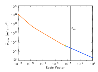
is shown in Figures 1 and 2.
The smooth transition between the two parts of the solution (early-time and late-time)
follows from the correctness of the matching conditions
(see Appendix LABEL:app:matching). The evolution of the SFDM energy
density in Figure 1
(left-hand plot) shows not only the transition of SFDM from CDM-like
to radiationlike around , but that at an even
earlier time , SFDM follows, indeed, a stiff equation
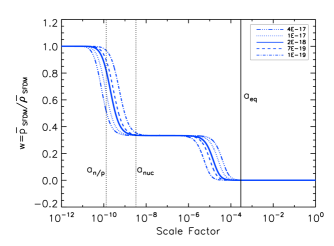
of state. The evolution of the equation of state is plotted in
Figure 1 (right-hand plot), where we can also
clearly see the transition from the stiff phase, to the radiationlike
phase, to the CDM-like phase.
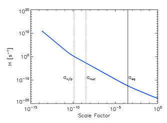
The evolution of the energy content in our fiducial model can be found in Figure 3. The energy density of SFDM surpasses that of radiation in the stiff phase of SFDM. Hence, the expansion rate in the stiff phase is higher, , than that in the radiation-dominated era, . This is a “scalar-field-dark-matter-dominated” era, before the radiation-dominated era. Here, the transition time from the stiff phase to the radiationlike phase depends on both and . This can be understood by realizing that, the transition happens when the first term (kinetic term, which depends on ) and the third term (self-interaction term, which depends on ) on the rhs of (12) and (12) become of equal order. Another way to see this is that, the equations which we solve when scalar field oscillation is slower than the Hubble expansion rate involve both these two parameters (see equations (III.3.1) and (III.3.1)). After the stiff-to-radiation transition, the energy fraction of SFDM reaches a “plateau” as well as that of the regular radiation component, since both components have radiationlike equations of state. This already implies that the kinetic term diminishes to the point where it is comparable to the self-interaction term (see equation(16)), as the scalar field oscillation becomes faster than the Hubble expansion rate, which is verified below. Therefore, the height of the plateau, i.e., the energy fraction of SFDM in the radiationlike phase, is determined by alone, because the equations for the fast oscillation approximation only concern this ratio (see equation (17)). It should be noted that the plateau height would vanish if there is no self-interaction (), see also Section V.4.
The energy fraction of SFDM starts to rise from the plateau value after a second transition from the radiationlike phase to the CDM-like phase. The energy density of SFDM evolves as like standard CDM, and the expansion rate as when SFDM dominates. The background evolution of the fiducial model is then the same as the basic model.
It is interesting to note that, in the SFDM model, dark matter dominates over the other cosmological components twice during the cosmic history, first in the stiff-matter phase, where it is highly relativistic, and later, when it behaves as pressureless dust, as in the standard scenario of CDM. As we will see in the next section, there are indeed constraints to be derived from both epochs. Also, the radiation-dominated era of the universe basically coincides with the radiationlike phase (plateau) of SFDM, since both of the SFDM transitions occur rapidly.

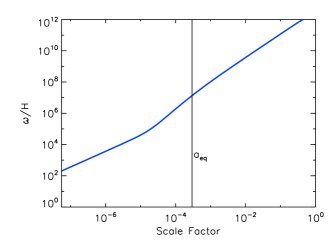
We would like to verify that the fast oscillation approximation discussed in Section III.2.1 is indeed applicable for the fiducial model, for large enough , where we solve for the evolution of the time-averages of and , instead of solving for their exact values. In other words, we would like to see that its condition is fulfilled during that era, for our fiducial model. The plot of can be found in Figure 2 (right-hand plot). Apparently, for all therein, justifying the fast oscillation approximation at later times.
IV Constraints on particle parameters from CMB and BBN measurements
IV.1 Constraint from
As has been noted before (Goodman; Peebles2000; ALS2002) the transition of SFDM from the radiationlike phase to the CDM-like phase must happen early enough to be in agreement with the redshift of matter-radiation equality determined by the CMB temperature power spectrum, since its shape is subject to the early integrated Sachs-Wolfe (ISW) effect, which depends upon HuSugiyama1995. In other words, in order to preserve , SFDM should be well into the CDM-like phase at . Before we proceed, it should be marked that the requirement above actually prohibits any freedom in choosing one of the initial conditions , the present-day SFDM density parameter, which must be the same as that in the six-parameter base model (see Table 1). In fact, one can derive from the definition of that
| (26) |
where is the scale factor at matter-radiation equality. This justifies our choice of .
The requirement that SFDM be fully non-relativistic at sets a constraint on the SFDM particle parameters, which is illustrated in Figure 1. The redshift of matter-radiation equality , according to Table 1, is marked as the vertical solid line in every plot. We define the cross in the left-hand plot to be the point at which (neglecting the subscript SFDM here) is 0.001, a tiny deviation from zero, and consider SFDM after this point as fully non-relativistic. We can see that for the fiducial model, this point is indeed early enough compared with . In fact, only the ratio is constrained by this requirement, as it alone determines the radiation-to-matter transition point of SFDM, resulting in
| (27) |
This is the upper bound which would make the cross in the left-hand plot of Figure 1 lie on top of the vertical line indicating , i.e., the marginal case where SFDM has just fully morphed into CDM at matter-radiation equality (see also the right-hand plot for the evolution of in the marginal case). Equation (27) implies that, even SFDM with large values of and , as adopted in some literature, is able to fulfill this constraint (this is in the self-interaction-dominated limit, since large indicates small ).
The choice of the threshold 0.001 is artificial, though. If we relax it to 0.01, i.e., consider SFDM as fully non-relativistic when is less than 0.01, the corresponding constraint on would become , allowing a broader range of values. To determine this threshold, we need to calculate the CMB power spectrum for given SFDM particle parameters and see the range of them that preserves the early ISW effect. We plan this for future work.
IV.2 Constraint from during big bang nucleosynthesis
The abundances of the big bang nucleosynthesis (BBN) products set a constraint on the Hubble expansion rate at that time, which depends on the total energy density of the relativistic species, parameterized by an effective number of relativistic degrees of freedom, also known as an effective number of neutrino species, (see Ref. Steigman2012 for a recent review). Thus, measurements of the primordial abundance of helium and deuterium can constrain the expansion rate or, equivalently, , during BBN. In the model, where there are only three SM neutrino species, NEFFS. In contrast, in SFDM model, if SFDM is relativistic then, it will contribute to as an extra relativistic component, and the constraints on consequently put control on the properties of SFDM, i.e., its particle parameters again.
The standard BBN scenario consists of two stages, the freeze-out of the neutron fractional abundance and the production of light elements combining free neutrons into nuclei, each affected by the expansion rate at its own epoch. The attempts to determine from BBN usually fit a cosmological model with constant extra number of neutrino species , e.g., with a constant portion of sterile neutrinos, to the primordial abundances of light elements extrapolated from observations. However, in SFDM, the caused by SFDM is changing over time as its equation of state varies during different eras. Therefore, we must study the evolution of throughout BBN, which is an extended period from the beginning of the neutron-proton ratio freeze-out around MeV (the difference between the neutron and the proton mass) to the epoch of nuclei production around MeV.
In a SFDM model, we infer the during BBN, namely from to , from the energy density of relativistic SFDM , which is determined by the particle parameters. In fact, SFDM is completely relativistic then and is the only source for ,
| (28) |
where is the total energy density of the SM neutrinos. We compare the obtained this way to the measured value (constant over time) and impose a conservative constraint that the during BBN be all the time within 1 of the measured value,
| (29) |
which we adopt from Ref. Steigman2012. We shall adopt this 68% confidence interval in constraining the parameters of SFDM in what follows. We note that while the standard CDM model with is inconsistent with the 1 constraint, it is, nevertheless, consistent within 95% confidence. Ideally, we need to fit our model not to such a constant value, but to the data of primordial abundances directly by deriving those for SFDM with a BBN code, which is intended as our future work.
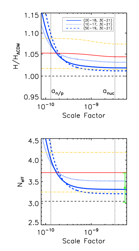
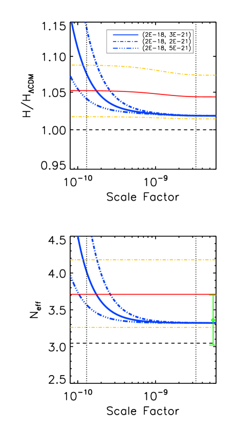
The result is plotted in Figure 4. The upper plots show the Hubble expansion rate of SFDM universes with different particle parameters normalized to the expansion rate of the basic universe, which is an equivalent illustration of the evolution of , as in the lower plots. The thin curves are benchmarks. The solid ones refer to a universe with a constant of the central value in equation (29) and the dash-dotted ones refer to such universes with of the 1 limits there, respectively. Note that in the upper plots for the normalized expansion rate, these thin curves are not straight lines due to the electron-positron annihilation. After this event, the neutrinos contribute less to the total energy density of the universe as their energy density fraction shrinks, because they are decoupled and do not get heated.
In each plot, the thick curves denote different models of (, ), according to the legend. The solid ones represent the fiducial model again: it complies with the constraint mentioned above (29). It can be seen that these curves all reach the “plateau”, i.e., the radiationlike phase, before the epoch of light-element production . The plateau height is purely determined by , as explained in Section III.3.2. In the left-hand plots, where we fix , the higher the , the higher the plateau. Meanwhile, earlier at the transition from the stiff phase to the radiationlike phase may not have finished and the value of can be higher than its plateau, which is a function of both and . In the right-hand plots, models with the same , but different , have the same plateau height, but diverge with a different rate as we go back in time: the lower the , the later is the transition to the radiationlike phase. Therefore, the evolution of during BBN restricts both SFDM particle parameters, and . This constraint is demonstrated in the next section and Figure 5.
Note that this constraint is also illustrated in Figure 3, where the definitions of the thin curves
between and , among which one is solid and two are dash-dotted,
are the same as above,
and the fraction of the SFDM energy density is restricted by the two dash-dotted curves,
which correspond to the 1 limits of in equation (29).
Again, these thin curves, which represent the energy fractions of extra radiation
in models with constant , slightly drop because of the electron-position annihilation.
While characterizes the SFDM energy density (see equation (28)), the relation between and
has a simple analytical form during the plateau. The total energy density of a SFDM universe during the radiation-dominated era is proportional to
{IEEEeqnarray}rl
& 2+2N_eff(plateau)⋅78(411)^4/3
= (2+2N_eff,standard⋅78(411)^4/3)×
×11-ΩSFDM(plateau).
Thus, if SFDM reaches the plateau before ,
the 68% confidence interval of (29) can be converted to that of during the plateau (its plateau height), using the equation above,
| (30) |
Consequently, we can use either (29) or (30) to constrain the SFDM parameter , in terms of the plateau height, of those models in which SFDM has reached the radiationlike phase by the end of BBN. The result is
| (31) |
as will be seen in Figure 5. It should be also heeded that, in principle, SFDM does not have to reach the plateau by , and the result above (31) is not applicable for those models.
IV.3 Result: allowed SFDM particle parameter space
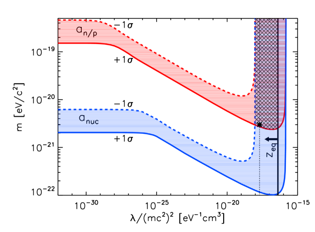
Combining the results from the above two sources of constraints, we can confine the allowed region in the parameter space of SFDM, or ultralight bosonic particle, see Figure 5 for the parameter space plot. The constraint from is given by the solid vertical line: the region on its left side is allowed, as shown by equation (27). For the constraint from during BBN, we sample the parameter space to obtain the critical parameter values which marginally fulfill the limits (29). The two shaded bands correspond to the constraints that be within 1 at and , as labeled respectively. For each band, the thick solid (dashed) boundary curve refers to the upper (lower) 1 limit of . The intersection of these two bands represents the range of parameters that is consistent with the constraint within throughout BBN. It is easily seen from the figure that all allowed choices of (, ) from the constraint indeed correspond to models in which SFDM has reached the radiationlike phase by the end of BBN, so that must be bounded within the asymptotic vertical lines (31) explained in the last section. This fact is completely due to the present-day measured value (29). Should the 68% confidence interval of be broaden, models in which SFDM had not reached the plateau by the end of BBN might also be allowed. Such models would not lie within the asymptotic vertical bounds of in the parameter space, as mentioned at the end of the last section.
The final allowed region is given by combining all the constraints, leaving the crosshatched area. The dotted vertical line, where the fiducial model sits, has the value , which corresponds to models with parameters for an equilibrium halo of size about 1 , see equation (32) in Section V.1. We can see that it lies within the allowed region, for high enough particle mass . The significance of this result will be discussed in Section V.1.
V discussion
V.1 Relation between and smallest dark matter structure
We mentioned in the introduction that standard CDM meets challenges on small scales (mainly the cuspy core problem and the missing satellites problem), which could be possibly resolved if dark matter clustering is prohibited below certain scales. As a matter of fact, it has been pointed out in previous literature, e.g., Refs. Goodman; BoehmerHarko2007; RS1, that self-interacting SFDM implies a minimum length scale for a virialized object. Though it is negligible compared with the energy density, as we pointed out in Section (1) (i.e., SFDM behaves as collisionless dust on large scales), this self-interaction pressure affects the dynamics of small-scale nonlinear structures in the dark matter, just as thermal gas pressure does for the baryons.
In fact, equation (19) is an polytropic equation of state , whose coefficient is proportional to . This is true even for the inhomogeneous case, if we replace the background and by local values. Therefore, the minimum length scale in the self-interaction-dominated limit is then given by the radius of a virialized polytrope
| (32) |
which is a function of only Goodman. Note that up to a factor of order unity, and it is more precise to use for purposes with regard to a virialized dark matter halo.
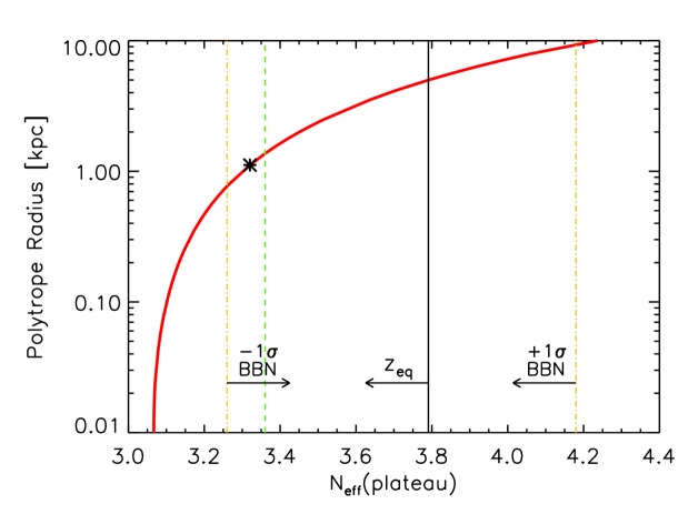
On the other hand, we have verified in Section IV.2 that as reaches the plateau (SFDM reaches the radiationlike phase), its value is also purely determined by . Therefore, we can plot the polytrope radius against corresponding to the plateau, revealing a hitherto unnoticed relation between the scale of the smallest dark matter structures and the number of relativistic species in the radiation-dominated era, see Figure 6.
The plot shows that higher implies stronger self-interaction pressure hence larger minimum scale for dark matter structure. The constraints discussed in the above section gives the allowed window of the minimum length scale, which is the segment of the curve between the left dotted vertical, the lower 1 limit from BBN measurement, and the solid vertical, the bound from the constraint on by , see equation (27). We can see that our fiducial model which corresponds to a minimum length scale of 1.1 kpc lies within the allowed window. It is a satisfactory result since this is about the scales where the small-scale CDM problems start to be significant from observations dB2001; Oh2008; Amorisco2012. We should also note that the allowed window for the minimum length scale is subject to changes in future observational results from CMB and BBN.
V.2 Imprints on the CMB from a time varying
Besides BBN, the angular power spectrum of the CMB temperature fluctuations can also be used to constrain the expansion rate of the universe during the radiation-dominated era by the ratio of the Silk damping scale to the sound horizon scale Planck. This provides a different constraint on from that described above from BBN. While the expansion rate depends upon the number of relativistic species present as well, it should be noted, though, that because of its possible evolution, the affecting the CMB power spectrum is not the same as the during BBN. The former concerns its value during the epoch spanned by the moment at which the smallest angular scale probed () enters the horizon, , to that of matter-radiation equality at , as pointed out in Ref. Bashinsky2004. By contrast, the BBN constraint probes at . In the SFDM model, evolves over time in such a way that is (at most) its plateau value at , and finally reduces to the standard value of 3.046 when SFDM becomes fully non-relativistic (before , as explained in Section IV.1). Therefore, the plateau value of during the radiation-dominated era serves as an upper bound for what is responsible for the expansion rate from to .
However, a complication arises that the ratio of does not only depend on the expansion rate during the period mentioned above, but also on the primordial Helium abundance , since the damping tail is subject to the number density of free electrons WMAP9. Actually,
| (33) |
where refers to the Hubble expansion rate between and . We also know that is dependent upon during BBN (an increase in results in a higher ). Therefore, the relativistic degrees of freedom suggested by CMB measurements, e.g., given by Planck+WP+highL Planck, (again, models with constant are fitted to the data) is in fact an imprint from both during BBN at early times (through ) and its later evolution from to (through ), in SFDM. In fact, equation (33) implies that increases when either or increases, provided a higher at the respective epoch, which then suggests that, given by CMB measurements be between the during BBN and the from to (the exact relation requires the calculation of linear growth). We then note that SFDM naturally provides an explanation for the difference between the values currently measured from BBN and CMB, in which the BBN value is larger than the CMB value.
V.3 Early stiff-matter phase
We have seen in Section III.2.2 that SFDM undergoes a stiff phase, when and . This feature of scalar fields has been noted before in models where the scalar field describes post-inflation universe or dark energy; see, e.g., Refs. RP1988; Joyce1997; CEM2007. In Ref. ALS2002, this feature has been found for SFDM without self-interaction. However, these authors did not find the accompanying constraint on the particle parameters, and also were limited to analytic treatment, while we calculated the evolution numerically and explore the parameter space where the stiff phase is important. The first suggestion of a stiff equation of state for the baryonic fluid in the early universe seems to be by Refs. Zeldovich1962; Zeldovich1972. The possibility of pre-BBN non-standard expansion histories, which includes a component decaying as , has been considered, e.g. in Refs. KT1990 and Dutta2010. However, the stiff components studied there do not undergo any transition, i.e., always decay as , unlike our model.
In a SFDM universe, the stiff phase can last until BBN occurs due to the constraints on the expansion rate. As we have seen in Section IV.2, for all viable models the stiff phase completely ends before . An interesting question is whether the stiff phase before will affect baryonic processes so as to leave an imprint on BBN products. In fact, the free neutron abundance is subject to beta decay, which happens ever since neutrons have existed, going as with the neutron decay time . Thus, the number of free neutrons left for nucleosynthesis depends on the age of the Universe, , since the QCD phase transition. Now, if in the stiff phase, instead of the radiation-era dependence, , this will change the number of available free neutrons before . The change in the age of the Universe is marginal, though, with a factor of , instead of , to multiply the decay-factor. As shown in the left-hand plot of Figure 2, the Hubble time at the epoch of the stiff-radiation transition is , which actually applies to all viable models. It is thus safe enough to constrain SFDM parameters only during BBN.
As far as the QCD phase transition is concerned, which happens somewhere between 150 – 300 MeV, there is still a lot of ongoing work to understand those processes in full. However, the relaxation time of the strong force is so tiny, in contrast to the Hubble time, that the QCD transition takes place in chemical equilibrium all the time, without a freeze-out timing issue. Therefore, we think the universe can be in the SFDM-dominated era in the stiff phase with a higher expansion rate, as suggested by our model, and yet accomplish a standard hadron era.
V.4 Implications for fuzzy dark matter
Our analysis above is valid for arbitrary value of . It is natural, therefore, to ask what the implications of our constraints are for the limiting case of . SFDM without self-interaction, , or fuzzy dark matter, is left with the quadratic potential in (5). Its popularity is reflected by numerous previous investigations; see, e.g., Refs. KMZ; Sin; Magana2012. One reason is that, even without the self-interaction pressure associated with nonzero , FDM still provides a mechanism to suppress structures on scales below , as a result of quantum pressure due to the Heisenberg Uncertainty Principle. Since it is an important special case of the model we have investigated, we devote this subsection to summarize the implications for this model from our analysis.
Without the self-interaction term, FDM has only two evolutionary phases, the early relativistic, stiff-matter phase, followed by the non-relativistic, CDM-like phase. For values of which are large enough to make this transition occur before the BBN epoch, the redshift of matter-radiation equality, , is unaffected because of the absence of the plateau (the radiationlike phase). Nevertheless, BBN sets a constraint on the only parameter left, the mass . Since the kinetic term in the SFDM energy density (12) goes inversely with , the transition between stiff and dust-like equation of state happens later with decreasing mass. In fact, according to Figure 5, if we accept the 1 limits on allowed by BBN to constrain , there is no value of for which can be consistent, which indicates a rejection of the FDM model at . We highlight this result, since FDM with eV/ has been a very popular candidate in the literature because the minimum length scale that corresponds to such particle mass is roughly 1 kpc, as mentioned in the introduction. Again, we should admit that, placing a less tight constraint, e.g., within 2, FDM may be able to fit BBN measurements.
VI Conclusions
We presented the cosmological evolution of a universe in which dark matter is comprised of ultralight self-interacting bosonic particles, which form a Bose-Einstein condensate, described by a classical complex scalar field (SFDM). We solved the Klein-Gordon and Einstein field equations for the time-dependence of an FRW universe with this form of dark matter, and placed constraints on the SFDM particle mass and self-interaction coupling strength (or equivalently ) from cosmological observations.
Unlike standard CDM, which is always non-relativistic once it decouples from the background, SFDM has an evolving equation of state. As a result, there are four eras in the evolution of a homogeneous SFDM universe: the familiar radiation-dominated, matter-dominated and Lambda-dominated eras common to standard CDM as well, but also an earlier era dominated by SFDM with a stiff equation of state. Then, and . The manifestation of this era does not depend on whether self-interaction has been included or not. It appears in fuzzy dark matter models with as well. The timing and longevity of this era (or the stiff phase of SFDM), however, depend on the particular values of SFDM particle parameters, along with . It is necessary to ensure that the stiff phase is ending when big bang nucleosynthesis begins. This finding is a special novelty of our analysis. At intermediate times, SFDM is radiationlike, with . Finally, SFDM must transition to the CDM-like phase before the epoch of matter-radiation equality, and thereafter behaves as a pressureless dust.
The effect of this SFDM equation of state evolution on the expansion rate and mass-energy content of the universe enables us to place constraints on and , by using at BBN, and measured by CMB anisotropy. We find that eV and . While we are able to place more stringent bounds on these particle parameters than the previous literature, there remains a large range of SFDM parameters which provides an expansion history in conformity with cosmological observations. Our investigations thereby contribute to previous efforts in establishing SFDM as a viable dark matter candidate. Work is in progress to study the linear and nonlinear growth of structures in a SFDM universe, in order to find out which part of the parameter space of SFDM is able to explain observations on all scales self-consistently.
Acknowledgements.
We are grateful for helpful discussions with Can Kilic, Dustin Lorshbough, Tonatiuh Matos and Eiichiro Komatsu. This work was supported in part by NSF grant AST-1009799 and NASA grant NNX11AE09G to PRS. TRD also acknowledges support by the Texas Cosmology Center of the University of Texas at Austin.Appendix A Basic equations in a perturbed Friedmann-Robertson-Walker metric
The general perturbed Friedmann-Robertson-Walker (FRW) metric in the comoving frame has the form
| (34) |
where the perturbed quantities , and are all .
A.1 Conformal Newtonian gauge
We can apply the conformal Newtonian Gauge if only scalar perturbations are permitted, where the metric reduces to MBW
| (35) |
or
The corresponding Christoffel symbols are Dodelson
| (36) |
A.2 Klein-Gordon equation
A.3 Einstein field equations and curvature tensor
The Einstein-Hilbert action is defined as
| (40) |
The Einstein field equations can be derived from the principle of
least action with variation in :
{IEEEeqnarray}rCl
0 & = δS_H
= ∫d^4x(δ(-gR)16πGc-4+δ(-gL))
= ∫d^4x(--g16πGc-4(R_μν-12g_μνR)+
+δ(-gL)δgμν)δg^μν.
Defining the energy-momentum tensor as
| (41) |
the field equations are thus
| (42) |
The Riemann curvature tensor is defined as
| (43) |
With the Christoffel symbols (36) we can calculate the diagonal Ricci tensors to first order in ,
Consequently the Ricci scalar is {IEEEeqnarray}rCl R & ≡ g