Tight Bounds for the Entanglement of Formation of Gaussian States

Abstract

We establish tight upper and lower bounds for the Entanglement of Formation of an arbitrary two-mode Gaussian state employing the necessary properties of Gaussian channels. Both bounds are strictly given by the Entanglement of Formation of symmetric Gaussian states, which are simply constructed from the reduced states obtained by partial trace of the original one.

I Introduction

A considerable effort has been devoted to the characterization of correlations contained in quantum states, or how much information two parts of the same system can share. The nature of these correlations can be classical or genuinely quantum, the last one being characterized by the presence of some sort of entanglement Horodecki et al. (2009). For pure bipartite states (states solely quantum correlated) this question was solved a long time ago: every measure of entanglement is completely equivalent to the von Neumann entropy of the reduced state of the bipartite system — It quantifies how much shared information the global system loses after a partial trace. On the other hand, when both kinds of correlations are present, i.e., when dealing with mixed states, it is impossible to know which kind of correlations were lost after the partial trace. The best we can do is to minimize over all possible quantum correlated state decompositions present in this mixed one — the process called as the convex roof of a measure. The convex roof of the von Neumann entropy is what we call Entanglement of Formation (EoF). Among all measures of entanglement the EoF plays a fundamental role: based on the principle that entanglement cannot increase under local operations it was shown that this measure is a lower bound for all suitable measures of entanglement Horodecki et al. (2000). Theoretically, the convex roof extension of a measure is very well defined, but in practice it is hard to solve. Only for a small class of states presenting special symmetries is it possible to express the EoF analytically Horodecki et al. (2009).

Gaussian states (GS) are remarkable states in physics, and in quantum information theory they are the natural candidates to implement quantum computation with continuous variable states Lloyd and Braunstein (1999). This argument is sufficient to understand the collective effort of the community to search for an analytical expression for GS EoF. The first step in that direction Giedke et al. (2003) considered symmetric Gaussian states (SGS), defined as states where both reduced partitions have equal purity or equal von Neumann entropies. Subsequently a definition of another convex roof extension — the Gaussian Entanglement of Formation (GeoF) appeared Wolf et al. (2004). There the minimization procedure is taken over a restricted set — the set of pure GS — and therefore is equal to the EoF when the state is symmetric. However no analytical expression was given: the process relies on a minimization of a polynomial function. Another important conceptual step was presented in Rigolin and Escobar (2004), where the authors found two distinct lower bounds to the EoF of GS and showed the importance of knowing at least analytical bounds for the EoF. More recently, the work Marian and Marian (2008) shows that the set used in the numerical minimization procedure to calculate the GoeF is indeed the correct one to find the EoF for a GS.

In this paper we show a new way to determine generic tight bounds for the EoF of an arbitrary GS. We use the very known concept of classical Gaussian channels Eisert and Wolf together with the desired convexity property of generic measures of entanglement. This paper is organized as follows: In Sec. II we define the set of GS and present some necessary concepts and quantities involved with the EoF calculation, whose properties are presented in Sec. III. In Sec. IV we review the definition of Gaussian channels and in Secs. V and VI we present our central results on the derivation of the limits to the EoF. Finally in Sec VII we present our conclusions and perspectives.

II Gaussian States

The covariance matrix (CM) of a genuine two-mode bipartite GS $\hat{\rho}_{\!{\mathbf{A}}{\!\mathbf{B}}}$ is defined by

$$\mathbf{V}_{\!\!{\mathbf{A}}{\!\mathbf{B}}}\equiv\left(\begin{array}[]{lc}\mathbf{A}&\mathbf{C}\\ \mathbf{C}^{\top}&\mathbf{B}\end{array}\right),$$ (1)

where $\mathbf{A},\mathbf{B},\mathbf{C}$ are $2\times 2$ block matrices, with $\mathbf{B}\geq\mathbf{A}\geq 0$, without loss of generality. As a manifestation of the Heisenberg uncertainty principle, this CM must regard the following (positivity semidefiniteness) inequality

$$\mathbf{V}_{\!\!{\mathbf{A}}{\!\mathbf{B}}}+i\mathsf{J}\geq 0\,\,\,\textrm{where}\,\,\,\mathsf{J}=\left(\begin{smallmatrix}0&1\\ -1&0\end{smallmatrix}\right)\oplus\left(\begin{smallmatrix}0&1\\ -1&0\end{smallmatrix}\right).$$ (2)

The generalization of this inequality for many-modes is trivial and only enhances the dimensions of the CM and $\mathsf{J}$.

Using unitary local operations (which do not change the degree of entanglement) we can reduce the above state to the so called standard form Simon (2000):

$$\mathbf{A}\mapsto a\,\mathsf{I}_{2},\,\,\,\mathbf{B}\mapsto b\,\mathsf{I}_{2}\,\,\,{\rm and}\,\,\,\mathbf{C}\mapsto{\rm Diag}\left(c_{1},c_{2}\right),$$ (3)

where $\mathsf{I}_{2}$ is the two dimensional identity matrix, $a,b\geq 1$ and, for simplicity, $c_{1}\geq|c_{2}|,\,\,c_{2}<0$. We also define the local symplectic invariants:

$$I_{1} \equiv \det\mathbf{A}=a^{2},\,\,\,I_{2}\equiv\det\mathbf{B}=b^{2},\,\,\ I_{3}\equiv\det\mathbf{C}=c_{1}c_{2},$$

$$I_{4} \equiv {\rm Tr}\left(\bf A\mathsf{J}\bf C\mathsf{J}\bf B\mathsf{J}C^{\top}\mathsf{J}\right)=ab(c_{1}^{2}+c_{2}^{2}).$$ (4)

Using the above definitions we are able to calculate the symplectic eigenvalues (SE) of the CM in (1), as in Serafini et al. (2004):

$$\mu_{\pm}=\sqrt{\tfrac{I_{1}+I_{2}}{2}+I_{3}\pm\sqrt{\left(\tfrac{I_{1}-I_{2}}{2}\right)^{2}+(I_{1}+I_{2})I_{3}+I_{4}}}.$$ (5)

We could also arrange them as a diagonal matrix, $\Lambda_{\mathbf{V}_{\!\!{\mathbf{A}}{\!\mathbf{B}}}}\equiv\mu_{-}\,\mathsf{I}_{2}\oplus\mu_{+}\,\mathsf{I}_{2}$, which we call symplectic spectrum. The imposition of (2) guaranties that a genuine physical state must obey $\mu_{+}\geq\mu_{-}\geq 1$.

When the CM (1) undergoes a partial transposition transformation, represented by the diagonal matrix $\mathbf{T}_{\!B}:=\mathsf{I}_{2}\oplus\hat{\sigma}_{z}$, where $\hat{\sigma}_{z}$ is the third Pauli matrix, it becomes $\widetilde{\mathbf{V}}_{\!\!{\mathbf{A}}{\!\mathbf{B}}}\equiv\mathbf{T}_{\!B}{\mathbf{V}}_{\!\!{\mathbf{A}}{\!\mathbf{B}}}\mathbf{T}_{\!B}^{\top}$. The net effect of this transposition is to change the signal of $c_{2}$ in (II), and the symplectic spectrum of $\widetilde{\mathbf{V}}_{\!\!{\mathbf{A}}{\!\mathbf{B}}}$ is simply obtained from (5) by the substitution $I_{3}\mapsto-I_{3}$:

$$\widetilde{\mu}_{\pm}=\sqrt{\tfrac{I_{1}+I_{2}}{2}-I_{3}\pm\sqrt{\left(\tfrac{I_{1}-I_{2}}{2}\right)^{2}-(I_{1}+I_{2})I_{3}+I_{4}}}.$$ (6)

Applying the Peres-Horodecki separability criteria Simon (2000) to the CM (1) a bipartite GS is entangled iff $\widetilde{\mu}_{-}<1$.

Let us define the CM of a SGS $\hat{\rho}_{{\mathbf{M}}{\!\mathbf{M}}}$ as

$$\mathbf{V}_{\!\!{\mathbf{M}}{\!\mathbf{M}}}\equiv\left(\begin{array}[]{lc}\mathbf{M}&\mathbf{C}\\ \mathbf{C}^{\top}&\mathbf{M}\end{array}\right),$$ (7)

i.e., Eq. (1) with ${\mathbf{A}}={\mathbf{B}}={\mathbf{M}}$ which under a local transformation $\mathbf{M}\mapsto m\,\mathsf{I}_{2}$. Its SE and the SE of its partial transposition are obtained from (5) and (6) and are, respectively, given by

$$\!\!\!\!\nu_{\pm}=\sqrt{I_{1}+I_{3}\pm\sqrt{I_{4}+2I_{1}I_{3}}}=\sqrt{(m\pm c_{1})(m\pm c_{2})}$$ (8)

and

$$\!\!\!\!\!\widetilde{\nu}_{\pm}=\sqrt{I_{1}-I_{3}\pm\sqrt{I_{4}-2I_{1}I_{3}}}=\sqrt{(m\pm c_{1})(m\mp c_{2})}.$$ (9)

As we will see in the next section the EoF for SGS is a monotonically decreasing function whose argument is the smaller eigenvalue in (9).

III Entanglement of Formation

The EoF for a mixed state $\hat{\rho}=\sum_{i}p_{i}|\psi_{i}\rangle\!\langle\psi_{i}|$ is constructed as the convex roof of the von Neumann entropy $S$ for pure states:

$${\rm EoF}(\hat{\rho})=\inf_{\{p_{i},\psi_{i}\}}\sum_{i}p_{i}S(\psi_{i}),$$ (10)

the set $\{p_{i},\psi_{i}\}$ indicates that the minimization runs over all physically possible decompositions of $\hat{\rho}$.

Among all properties of the EoF defined above two of them will be very important for us: locality and convexity Horodecki et al. (2009, 2000). The locality states that the action of a local operation cannot increase the EoF. Furthermore, the EoF does not change under unitary local operations, which may be summarized as: if $\hat{U}_{L}$ is a local unitary operator, then

$${\rm EoF}\left(\hat{\rho}\right)={\rm EoF}\left(\hat{U}_{L}\,\hat{\rho}\,\hat{U}_{L}^{{\dagger}}\right).$$ (11)

Now, let us define a set of $N$ real numbers $0\leq\alpha_{i}\leq 1\,\forall i$, such that $\sum_{i=1}^{N}\alpha_{i}=1$ so that one can construct a convex decomposition of $\hat{\rho}$ into a set of density matrices $\hat{\rho}_{i}$. The convexity of the EoF implies that

$${\rm EoF}\left(\sum_{i=1}^{N}\alpha_{i}\hat{\rho}_{i}\right)\leq\sum_{i=1}^{N}\alpha_{i}\,{\rm EoF}\left(\hat{\rho}_{i}\right).$$ (12)

Working directly on formula (10), using the above two properties and the von Neumannn entropy of squeezed states, the authors in Refs. Giedke et al. (2003) could obtain an analytical formula for the EoF of any two mode SGS as

$${\rm EoF}(\hat{\rho}_{{\mathbf{M}}{\!\mathbf{M}}})=f\left(\tilde{\nu}_{-}\right),$$ (13)

where $\tilde{\nu}_{-}$ is the symplectic eigenvalue of the partially transposed CM $\widetilde{\mathbf{V}}_{\!\!{\mathbf{M}}{\!\mathbf{M}}}$ and the monotonically decreasing function $f$ is defined as $f(x)=c_{+}(x){\rm ln}(c_{+}(x))-c_{-}(x){\rm ln}(c_{-}(x))$ with $c_{\pm}(x)=(x^{-1/2}\pm x^{1/2})^{2}/4$. An attempt to generalize (13) for non-SGS with CM ${\mathbf{V}}_{\!\!{\mathbf{A}}{\!\mathbf{B}}}$ is given by the adoption of the function $f$ of (13) with $\tilde{\mu}_{-}$ defined in (5) as the argument, we call this quantity EeoF:

$${\rm EeoF}(\hat{\rho}_{{\!\mathbf{A}}{\!\mathbf{B}}})=f\left(\tilde{\mu}_{-}\right).$$ (14)

In Refs. Adesso and Illuminati (2007); Serafini et al. (2004) the authors conjecture that this should be the expression of the true EoF for GS, but here we will argue in the next sections that this quantity can be considered an estimation for the EoF.

It is possible to define a bona fide measure of entanglement even when the states $|\psi_{i}\rangle$ into the decomposition in (10) are taken to be Gaussian Wolf et al. (2004). This measure is known as Gaussian Entanglement of Formation (GeoF) and there isn’t an analytical expression for it. Indeed, it should be calculated by a minimization of a polynomial function whose coefficients are cumbersome functions of the entries of the matrix ${\mathbf{V}}_{\!\!{\mathbf{A}}{\!\mathbf{B}}}$ and are explicitly written in Ref. Adesso and Illuminati (2007). As a matter of fact, in Ref. Marian and Marian (2008) the authors show that the GeoF is the EoF for Gaussian states.

IV Gaussian Channels

The Gaussian channels (GC) considered here are trace preserving and completely positive maps acting on density operators, preserving also the Gaussian character of a state of this kind Eisert and Wolf ; Caruso et al. (2008). We will only concern ourselves with the classical noise channel (CNC), whose action on a density operator can be written as a convolution of the density operator with a Gaussian Caves and Wodkiewicz , i.e.,

$$\hat{\rho}=\frac{1}{(2\pi)^{2}}\int^{+\infty}_{-\infty}\frac{{\rm e}^{-\frac{1}{\hbar}\xi\cdot\Delta^{-1}\xi}}{\sqrt{\rm Det\Delta}}\,\,\hat{T}_{\xi}\hat{\rho}_{0}\hat{T}_{\xi}^{\dagger}\,\,\,d^{4}\xi.$$ (15)

The operators $\hat{T}_{\xi}$ are the Weyl displacement operators de Almeida (1998). The vector $\xi\in\mathbb{R}^{4}$ and $\Delta$ must be a positive semidefinite matrix, $\Delta\geq 0$. Physically, the noise channel may be implemented as the interaction of the system with a thermal bath at high temperature.

Concerning the CM of the states involved in (15), it is easy to show that if $\hat{\rho}_{0}$, which not necessarily Gaussian, has a CM $\mathbf{V}_{0}$, the state $\hat{\rho}$ will have the CM

$$\mathbf{V}=\mathbf{V}_{0}+\Delta.$$ (16)

Since the sum of positive semidefinite matrix is positive semidefinite, if $\mathbf{V}_{0}$ obeys (2), then $\mathbf{V}$ also will. From Eq. (15) one can see that it is a convex sum of operators once

$$\frac{{\rm e}^{-\frac{1}{2}\xi\cdot\Delta^{-1}\xi}}{\sqrt{\rm Det\Delta}}\geq 0\,\,\,{\rm and}\,\,\,\int^{+\infty}_{-\infty}\frac{{\rm e}^{-\frac{1}{2}\xi\cdot\Delta^{-1}\xi}}{(2\pi)^{2}\sqrt{\rm Det\Delta}}\,\,d^{4}\xi=1.$$ (17)

Now one can use Eq. (12) for the convex sum in (15) and the locality of the Weyl operator, Eq. (11), to show that

$${\rm EoF}\left(\hat{\rho}\right)\leq{\rm EoF}\left(\hat{\rho}_{0}\right).$$ (18)

In such a way, one can conclude that

$$\mathbf{V}=\mathbf{V}_{0}+\Delta\Longrightarrow{\rm EoF}\left(\hat{\rho}\right)\leq{\rm EoF}\left(\hat{\rho}_{0}\right),\,\,\,\forall\Delta\geq 0.$$ (19)

This equation is the principal statement of the present work, it will be useful for finding lower and upper bounds for the EoF of a general GS and it has a clear physical interpretation: as the channel adds noise to the system, there is no strangeness if the quantum correlations diminish.

V Bounds for EoF

Let us consider two SGS, $\hat{\rho}_{{\mathbf{N}}{\!\mathbf{N}}}$, $\hat{\rho}_{{\mathbf{M}}{\!\mathbf{M}}}$, whose CV are of the form (7) and a non symmetric one, $\hat{\rho}_{{\!\mathbf{A}}{\!\mathbf{B}}}$, whose CV is of the form given in (1). Mind that in our notation, all of the above states have a CM with the same block matrix $\mathbf{C}$. Suppose the following order to the matrices:

$$\mathbf{N}\geq\mathbf{B}\geq\mathbf{A}\geq\mathbf{M}.$$ (20)

Now we are able to find bounds for the EoF of a generic GS $\hat{\rho}_{\!\mathbf{A}\!\mathbf{B}}$. First, let us define two noise matrices $\Delta_{1}\equiv(\mathbf{N}-\mathbf{A})\oplus(\mathbf{N}-\mathbf{B})$ and $\Delta_{2}\equiv(\mathbf{A}-\mathbf{M})\oplus(\mathbf{B}-\mathbf{M})$, both are positive semidefinite regarding the ordering imposed in (20). It is easy to see that

$$\mathbf{V}_{\!\!{\mathbf{N}}{\!\mathbf{N}}}=\mathbf{V}_{\!\!{\mathbf{A}}{\!\mathbf{B}}}+\Delta_{1}\,\,\,\,\,\,\text{and}\,\,\,\,\,\,\mathbf{V}_{\!\!{\mathbf{A}}{\!\mathbf{B}}}=\mathbf{V}_{\!\!{\mathbf{M}}{\!\mathbf{M}}}+\Delta_{2},$$ (21)

therefore using the statement in (19), we can sort the EoF for the states as

$${\rm EoF}\left(\hat{\rho}_{\mathbf{N}\!\mathbf{N}}\right)\leq{\rm EoF}\left(\hat{\rho}_{\!\mathbf{A}\!\mathbf{B}}\right)\leq{\rm EoF}\left(\hat{\rho}_{\mathbf{M}\!\mathbf{M}}\right).$$ (22)

The advantage of the limiting bounds can be seen by the fact that they are the EoF of SGS and can easily be calculated by (13). Note that the Gaussian channels described by the noise matrices in (21) are non unitary operations but Gaussian and local (GLOCC).

As a matter of fact, until now we needed to assume that $\hat{\rho}_{{\mathbf{M}}{\!\mathbf{M}}}$ in (22) represents a genuine physical state in the sense of Eq. (2). In view of the sum of positive semidefinite matrices, Eq. (21) implies

$$\mathbf{V}_{\!\!{\mathbf{N}}{\!\mathbf{N}}}+i\mathsf{J}\geq\mathbf{V}_{\!\!{\mathbf{A}}{\!\mathbf{B}}}+i\mathsf{J}\geq\mathbf{V}_{\!\!{\mathbf{M}}{\!\mathbf{M}}}+i\mathsf{J}\geq 0,$$ (23)

which means that the physicality imposed on the lower matrix guarantees the physicality for all the others.

As a corollary of the result (22), the EoF of a non symmetric Gaussian state GS with CV (1) has two natural bounds

$${\rm EoF}(\hat{\rho}_{{\!\mathbf{B}}{\!\mathbf{B}}})\leq{\rm EoF}\left(\hat{\rho}_{\!\mathbf{A}\!\mathbf{B}}\right)\leq{\rm EoF}(\hat{\rho}_{{\mathbf{A}}{\!\mathbf{A}}}),$$ (24)

since

$$\mathbf{V}_{\!\!{\mathbf{A}}{\!\mathbf{B}}} = \mathbf{V}_{\!\!{\mathbf{A}}{\!\mathbf{A}}}+{\bf 0}_{2}\oplus({\mathbf{B}}-{\mathbf{A}})\,\,\,\text{and}\,\,\,$$

$$\mathbf{V}_{\!\!{\mathbf{B}}{\!\mathbf{B}}} = \mathbf{V}_{\!\!{\mathbf{A}}{\!\mathbf{B}}}+({\mathbf{B}}-{\mathbf{A}})\oplus{\bf 0}_{2},$$ (25)

where ${\bf 0}_{2}$ is the $2\times 2$ null matrix. In figure 1, one can see the GeoF for a non symmetric Gaussian state $\hat{\rho}_{\!\mathbf{A}\!\mathbf{B}}$, calculated by the recipe of Wolf et al. (2004); Adesso and Illuminati (2007) (remember that following Marian and Marian (2008), this GeoF must be the true EoF for GS) bounded by the EoF of SGs $\hat{\rho}_{\!\mathbf{A}\!\mathbf{A}}$ and $\hat{\rho}_{\mathbf{B}\!\mathbf{B}}$.

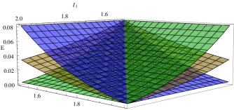
Figure 1: GeoF function (orange) bounded by the EoF of symmetric states (blue and green) as a function of the local symplectic invariants $I_{1}$ and $I_{2}$. The other invariants are chosen to guarantee the existence and entanglement of the states: $I_{3}=-0.2$ and $I_{4}=2|I_{3}|\sqrt{I_{1}I_{2}}$.

Comparing the EPR-uncertainties Giedke et al. (2003) of mixed GSs and of squeezed states, the authors in Rigolin and Escobar (2004) obtained the EoF for a SGS $\hat{\sigma}$ whose CM is like (7) with $\mathbf{M}=(\mathbf{A}+\mathbf{B})/2$ as a lower bound for the EoF of the general GS (1): ${\rm EoF}\left(\hat{\sigma}\right)\leq{\rm EoF}\left(\hat{\rho}_{\!\mathbf{A}\!\mathbf{B}}\right)$. It is impossible to deduce this bound using (22) since we can not construct $\Delta_{1}$ and $\Delta_{2}$ preserving positive semidefiniteness. However, $\mathbf{A}\leq\mathbf{M}=(\mathbf{A}+\mathbf{B})/2\leq\mathbf{B}$; then comparing the CM of the states using (19) with $\hat{\rho}=\hat{\rho}_{\mathbf{B}\!\mathbf{B}}$, $\hat{\rho}_{0}=\hat{\sigma}$ and $\Delta=(\mathbf{B}-\mathbf{M})\oplus(\mathbf{B}-\mathbf{M})$, one can establish its value on the hierarchy of (24) as

$${\rm EoF}\left(\hat{\rho}_{\mathbf{B}\!\mathbf{B}}\right)\leq{\rm EoF}\left(\hat{\sigma}\right)\leq{\rm EoF}\left(\hat{\rho}_{\!\mathbf{A}\!\mathbf{B}}\right)\leq{\rm EoF}\left(\hat{\rho}_{\!\mathbf{A}\!\mathbf{A}}\right).\!$$ (26)

The closer lower bound given above is always a physical state Rigolin and Escobar (2004) which is the best lower bound allowed by our method, i.e., any attempt to find a SGS with EoF closer to ${\rm EoF}\left(\hat{\rho}_{\!\mathbf{A}\!\mathbf{B}}\right)$ and smaller than ${\rm EoF}\left(\hat{\sigma}\right)$ fails to find a positive semidefinite $\Delta_{1}$ in (21).

Furthermore, given an arbitrary Gaussian state, some available relation between the local covariance matrices can be used to determine other bounds for the EoF of the original state, e.g., suppose ${\mathbf{B}}-{\mathbf{A}}\leq{\mathbf{A}}$, then the symmetric state $\hat{\rho}_{\mathbf{M}\!\mathbf{M}}$ with $\mathbf{M}={\mathbf{B}}-{\mathbf{A}}$ constitutes an upper bound to the state $\hat{\rho}_{\!\mathbf{A}\!\mathbf{B}}$. As a final comment, nothing prevents the nonphysicality (even the nonpositivity) of the operator $\hat{\rho}_{\!\mathbf{A}\!\mathbf{A}}$ in (24) when constructed from (1). Remembering that in our protocol all the matrices have the same correlation matrix $\mathbf{C}$, see Eqs. (1) and (7), one way to detour this undesired behavior is to search for another SGS described by a CM $\mathbf{V}^{\prime}$ with a different correlation matrix but with $\Delta^{\prime}=\mathbf{V}_{\!\!{\mathbf{A}}{\!\mathbf{B}}}-\mathbf{V}^{\prime}\geq 0$.

VI Estimation for EoF

Actually, we can derive a more general and mathematical precise procedure independent of Gaussian channels and physical states to determine an estimation for the EoF. This criterion for the EoF functions is a direct consequence of the Williamson theorem de Gosson and Luef (2009): considering two positive semidefinite matrices, $\mathbf{H}_{1}\geq\mathbf{H}_{2}$, their symplectic spectrum must be sorted as $\Lambda_{\mathbf{H}_{1}}\geq\Lambda_{\mathbf{H}_{2}}$. Assuming $f$ as a monotonically decreasing function, like the function defined below Eq. (13), one can see that

$${\mathbf{H}_{1}}\geq{\mathbf{H}_{2}}\Longrightarrow\tilde{\mathbf{H}}_{1}\geq\tilde{\mathbf{H}}_{2}\Longrightarrow f(\tilde{\nu}^{-}_{2})\geq f(\tilde{\nu}^{-}_{1}),$$ (27)

where $\tilde{\mathbf{H}}_{i}=\mathbf{T}_{\!B}\mathbf{H}_{i}\mathbf{T}_{\!B}$ is the partial transposition of the matrix ${\mathbf{H}_{i}}$ already defined and $\tilde{\nu}^{-}_{i}$ is the smaller symplectic eigenvalue of the matrix $\tilde{\mathbf{H}}_{i}$.

The statement of Eq. (27) is sufficient to prove that the function ${\rm EeoF}(\hat{\rho}_{\!\mathbf{A}\!\mathbf{B}})$ defined in (14) is also bounded exactly as ${\rm EoF}(\hat{\rho}_{\!\mathbf{A}\!\mathbf{B}})$ in (26) by the EoF of the same symmetric states. To see this let us take a look at the situation in Eq. (23),

$$\mathbf{V}_{\!\!{\mathbf{N}}{\!\mathbf{N}}}\geq\mathbf{V}_{\!\!{\mathbf{A}}{\!\mathbf{B}}}\geq\mathbf{V}_{\!\!{\mathbf{M}}{\!\mathbf{M}}}\Longrightarrow\widetilde{\mathbf{V}}_{\!\!{\mathbf{N}}{\!\mathbf{N}}}\geq\widetilde{\mathbf{V}}_{\!\!{\mathbf{A}}{\!\mathbf{B}}}\geq\widetilde{\mathbf{V}}_{\!\!{\mathbf{M}}{\!\mathbf{M}}},$$ (28)

which implies by (27) that $f(\tilde{\nu}^{-}_{\mathbf{M}})\geq f(\widetilde{\mu}_{-})\geq f(\tilde{\nu}^{-}_{\mathbf{N}})$ where $\widetilde{\mu}_{-}$ is the symplectic eigenvalue defined in (6) of $\widetilde{\mathbf{V}}_{\!\!{\mathbf{A}}{\!\mathbf{B}}}$ and $\tilde{\nu}^{-}_{\mathbf{M}}$ and $\tilde{\nu}^{-}_{\mathbf{N}}$ are the SE in (9) of the symmetric states $\hat{\rho}_{\mathbf{M}\!\mathbf{M}}$ and $\hat{\rho}_{\mathbf{N}\!\mathbf{N}}$. Obviously this works for the natural bounds (24). It is interesting to note that even knowing that the EeoF is not the true EoF for GS Marian and Marian (2008), it is bounded as if it were and this may be used to consider the EeoF as a good estimation for the true one. Numerical exploitations show that the estimation can be greater or smaller than the GeoF.

Needless to say, the statement in (27) can be used to sort and determine some bounds, e.g., the ordering ${\rm EoF}\left(\hat{\rho}_{\mathbf{B}\!\mathbf{B}}\right)\leq{\rm EoF}\left(\hat{\sigma}\right)$ in Eq. (26) can be attained if one compares the SEs associated with the partially transposed states.

VII Conclusions

Starting with the convexity property of the EoF, we describe a simple method to construct lower and upper bounds to the Entanglement of Formation for general Gaussian states which has a clear physical interpretation in terms of the action of a noise channel. The same procedure is used to define what we called natural bounds since they are constructed using only the one-mode reduced CM of a two-mode GS. We have also demonstrated that the same bounds can be applied to the generalization of EoF, where it is considered a monotonically decreasing function of the smaller symplectic eigenvalue — since we can not define it as a lower or an upper bound, we call it an estimation of the EoF (or the EeoF). For this we used the Williamson theorem for positive definite matrices, highlighting the underlying mathematical character of the EeoF. We strongly believe that these results can be used in the direction to obtain a closed and analytical formula for the EoF of general (nonsymmetric) Gaussian states. This is currently under investigation.