Probing the Higgs Portal at the LHC
Through Resonant di-Higgs Production

Abstract

We investigate resonant di-Higgs production as a means of probing extended scalar sectors that include a 125 GeV Standard Model-like Higgs boson. For concreteness, we consider a gauge singlet Higgs portal scenario leading to two mixed doublet-singlet states, $h_{1,2}$. For $m_{h_{2}}>2m_{h_{1}}$, the resonant di-Higgs production process $pp\to h_{2}\to h_{1}h_{1}$ will lead to final states associated with the decaying pair of Standard Model-like Higgs scalars. We focus on $h_{2}$ production via gluon fusion and on the $b{\bar{b}}\tau^{+}\tau^{-}$ final state. We find that discovery of the $h_{2}$ at the LHC may be achieved with $\buildrel<\over{{}_{\sim}}$ 100 fb^-1 of integrated luminosity for benchmark parameter choices relevant to cosmology. Our analysis directly maps onto the decoupling limits of the Next-to-Minimal Supersymmetric Standard Model (NMSSM) and more generically onto extensions of the Standard Model Higgs sector in which a heavy scalar produced through gluon fusion decays to a pair of Standard Model-like Higgs bosons.

I Introduction.

Both ATLAS and CMS observe a Standard Model-like Higgs boson with $\sim$125 GeV mass. While ongoing analyses show that the properties of the newly discovered particle are close to those expected for the Standard Model (SM) Higgs boson $h$, the full structure of the scalar sector responsible for electroweak symmetry-breaking remains to be determined. It is particularly interesting to ascertain whether the scalar sector consists of only one SU(2)_L doublet ($H$) or has a richer structure containing additional states. Addressing this question is an important task for future studies at the Large Hadron Collider.

An interesting avenue for the observation of additional scalar states $X$ occurs in Higgs portal scenarios that contain operators of the form $XH^{\dagger}H$ and $X^{2}H^{\dagger}H$. For $m_{X}>2m_{h}$, these operators enable the process $pp\to X^{0}\to hh$, where $X^{0}$ is the neutral component of $X$, if $X$ is not inert with respect to the Standard Model. Signatures of such resonant di-Higgs production are multiparticle final states comprised of the conventional Higgs boson decay products. Di-Higgs production also occurs purely within the SM, though it cannot receive any enhancement due to an intermediate resonance (for studies of Higgs self-coupling probes with di-Higgs production at the LHC, see Djouadi:1999rca ; Baur:2002qd ; Baur:2003gpa ; Baur:2003gp ; Dolan:2012rv ; Papaefstathiou:2012qe ; Goertz:2013kp ; Barr:2013tda ).

Higgs portal scenarios are strongly motivated by cosmology. In the presence of a discrete $Z_{2}$ symmetry, $X^{0}$ may be a dark matter candidate. In this case, the cubic operator is forbidden, the vacuum expectation value (vev) of $X^{0}$ vanishes, and resonant di-Higgs production cannot occur. In the absence of a $Z_{2}$ symmetry, however, both the cubic operator and a non-vanishing $X^{0}$ vev can exist. Under these conditions, the presence of the $X^{0}$ may facilitate a strong first order electroweak phase transition (EWPT) as required by electroweak baryogenesis (EWBG) (for a recent review, see Morrissey:2012db ). In this case, one would encounter a pair of neutral mass eigenstates $h_{1,2}$ formed from mixtures of the two neutral scalar fields, and for $m_{h_{2}}\geq 2m_{h_{1}}$ resonant di-Higgs production could proceed (see also Dolan:2012ac ).

In what follows, we investigate the prospects for observing such Higgs portal-mediated resonant di-Higgs production in the context of the simplest extension of the SM scalar sector involving one real gauge singlet, $S$. This “xSM” scenario can give rise to a strong first order electroweak phase transition as needed for electroweak baryogenesis in regions of parameter space that would also enable resonant di-Higgs production Profumo:2007wc ; Espinosa:2011ax ). Study of the xSM also allows for a relatively general analysis of Higgs portal mediated resonant di-Higgs production. In particular the present analysis can be mapped directly onto the “decoupling limit” $m_{A}\gg v$ of the Next-to-Minimal Supersymmetric Standard Model (NMSSM) Ellwanger:2009dp as well other scenarios that include additional degrees of freedom not directly relevant to di-Higgs production.

In this study, we concentrate on the $b{\bar{b}}\tau^{+}\tau^{-}$ final state, motivated in part by the analogous work on SM-only non-resonant di-Higgs production as well as by the considerations discussed in section IV. We find that with an appropriate strategy for background reduction, discovery of $h_{2}$ at the LHC may be feasible with $\sim$ 50 - 100 fb^-1. Other final states resulting from combinations of Higgs decay products may also provide promising probes of the Higgs portal through resonant di-Higgs production, and we defer an analysis of these possibilities to future work.

The discussion of our analysis leading to this conclusion is organized as follows. In Section II we review the theoretical framework and motivation for the xSM. Section III gives the present LHC constraints and discusses other phenomenological considerations. In Section IV we discuss the details and present the results of our LHC simulations and analysis, while in Section V we discuss their implications.

II Singlet Scalars Beyond the SM

Singlet scalar extensions of the SM are both strongly motivated and widely studied O'Connell:2006wi . In the present instance, we rely on the simplest version as a paradigm for Higgs portal interactions and the prospects for novel collider signatures. At the same time, singlet extensions of the scalar sector are interesting in their own right. From a model-building perspective, singlet scalars arise in various SM extensions, such as those containing one or more additional U(1) groups that occur in string constructions or variants on the NMSSM. Cosmology provides additional motivation. As noted above, the presence of the singlet scalar can enable a strongly first order EWPT as needed for electroweak baryogenesis, while imposing a $Z_{2}$ symmetry on the potential allows the singlet scalar to be a viable dark matter candidate (for early references, see, e.g. Refs. McDonald:1993ex ; Burgess:2000yq ). In principle, one may achieve both a viable dark matter candidate and a strongly first order EWPT for a complex scalar singlet extension in the presence of a spontaneously- and softly-broken global U(1) Barger:2008jx ; Gonderinger:2012rd .

In what follows, we concentrate on the real singlet, though many of the features discussed below will apply to the real component of the complex singlet case as well. The corresponding scalar potential for the SM Higgs doublet $H$ and a real singlet scalar field $S$ is

$$V(H,S)=-\mu^{2}\left|H\right|^{2}+\lambda\left|H\right|^{4}+\frac{b_{2}}{2}S^{2}+\frac{b_{4}}{4}S^{4}$$

$$+\frac{a_{2}}{2}S^{2}\left|H\right|^{2}+\frac{a_{1}}{2}S\left|H\right|^{2}+\frac{b_{3}}{3}S^{3}-\frac{a_{1}\,v^{2}}{4}S$$ (1)

We note that the scalar potential of a general NMSSM in the decoupling regime $m_{A}\gg v$ ($m_{A}$ is the mass of the neutral pseudocsalar) is precisely of the form (II) Ellwanger:2009dp , so our analysis for the xSM could be directly mapped into that interesting scenario (recent global fits of LHC data in the context of supersymmetric models tend to favor this regime Espinosa:2012in ; Barbieri:2013hxa ; Belanger:2013xza ). Studies of resonant di-Higgs production, though in a different context from the present one, have also been carried out Ellwanger:2013ova ; Cao:2013si ; Kang:2013rj .

Following Barger:2007im , we have incorporated the last term in (II) in order to cancel the singlet tadpole generated once the EW symmetry is spontaneously broken, with

$$H=\frac{1}{\sqrt{2}}\left(\begin{array}[]{c}0\\ h+v\end{array}\right)$$ (2)

in the unitary gauge and with $v=246$ GeV. Denoting the neutral component of $H$ by $H^{0}$, the minimization conditions $\partial V/\partial H^{0}=0$ and $\partial V/\partial S=0$ with lead to

$$H^{0}\bigl{[}-2\mu^{2}+4\lambda(H^{0})^{2}+a_{2}S^{2} + a_{1}S\bigr{]}=0$$ (3)

$$S\left[b_{2}+b_{3}S+b_{4}S^{2}+a_{2}(H^{0})^{2}\right] = \frac{a_{1}}{2}\left[v^{2}/2-(H^{0})^{2}\right]\ \ .$$

For positive $b_{2-4}$ and $a_{2}$, $H$ as given in (2), and $\lambda v^{2}=\mu^{2}$ as in the Standard Model, the scalar singlet does not develop a zero-temperature vev. The resulting mass term in the potential is

$$V_{\mathrm{mass}}=\frac{1}{2}\left(\begin{array}[]{cc}h&S\end{array}\right)\left(\begin{array}[]{cc}\lambda v^{2}&a_{1}v/2\\ a_{1}v/2&b_{2}+a_{2}v^{2}/2\end{array}\right)\left(\begin{array}[]{c}h\\ S\end{array}\right)\ .$$ (4)

The states $h$ and $S$ will mix after EWSB if $a_{1}\neq 0$, with mixing angle denoted by $\theta$. The mass eigenstates $h_{1,2}$ can then be expressed in terms of $h$ and $S$ as

$$\left(\begin{array}[]{c}h_{1}\\ h_{2}\end{array}\right)=\left(\begin{array}[]{cc}c_{\theta}&s_{\theta}\\ -s_{\theta}&c_{\theta}\end{array}\right)\,\left(\begin{array}[]{c}h\\ S\end{array}\right)\ \ \ ,$$ (5)

where $c_{\theta}\equiv\cos\theta$ and $s_{\theta}\equiv\sin\theta$ with

$$\tan\theta=\frac{x}{1+\sqrt{1+x^{2}}}$$ (6)

and

$$x=\frac{a_{1}v}{(\lambda-a_{2}/2)v^{2}-b_{2}}\ \ \ .$$ (7)

The corresponding masses are

$$m_{\pm}^{2} = \frac{1}{2}\left[(\lambda+a_{2}/2)v^{2}+b_{2}\right]$$

$$\pm\frac{1}{2}{\bigl{|}}(\lambda-a_{2}/2)v^{2}-b_{2}{\bigr{|}}\sqrt{1+x^{2}}$$

with $m_{2}=m_{+}$ and $m_{1}=m_{-}$.

The scalar potential (II) may then be written in terms of the following seven independent parameters: the two scalar masses $m_{1,2}$; the mixing angle $\theta$; $v$, $a_{2}$, $b_{3}$ and $b_{4}$. Henceforth, we assume that $h_{1}$ is the Higgs-like state currently being observed at the LHC, with $m_{1}=125$ GeV, and $h_{2}$ is a heavier scalar state with $m_{2}>2m_{1}$. The quartic coupling $b_{4}>0$ is needed to assure stability of the potential along the $S$ direction. The value of the effective trilinear $h_{2}h_{1}h_{1}$ coupling

$$\lambda_{211}=b_{3}s_{\theta}^{2}c_{\theta}+a_{2}vs_{\theta}(c_{\theta}^{2}-s_{\theta}^{2}/2)$$

$$\ +\frac{a_{1}}{4}c_{\theta}(c^{2}_{\theta}-2s^{2}_{\theta})-3\lambda vc^{2}_{\theta}s_{\theta}$$ (9)

is clearly of vital importance to our analysis. Note that $\lambda$ and $a_{1}$ are implicitly functions of $m_{1,2}$, $\theta$, $v$ and $a_{2}$ via Eqs. (6-II).

Considerations of the vacuum structure of the potential introduce constraints on the independent parameters of the potential. Tree-level stability for large values of the fields $h$ and $S$ is ensured for positive $\lambda$, $b_{4}$ and $a_{2}$. However, allowing $a_{2}<0$ can enable a strong first order electroweak phase transition Profumo:2007wc . In this case, requiring $4\lambda b_{4}>a_{2}^{2}$ maintains stability of the potential. This criterion becomes dependent on the cut-off of the low-energy effective theory after one takes into account the renormalization group evolution of the parameters, a consideration that we do not implement here (see, e.g., Gonderinger:2012rd and references therein). Note that for $a_{2}<0$ and/or $H$ different from (2), one may encounter additional solutions to (3) for which the $S$ vev does not vanish. We require that if such additional minima exist, the $\langle S\rangle=0$ extremum is a the global minimum. As illustrated in Fig. 1, doing so leads to the constraints in the $(a_{2},b_{3})$ plane for given values of $m_{1,2}$, $\theta$, and $b_{4}$. From Eq. (II) and the global stability region of Fig. 1, we then observe that for each value of $a_{2}$ there exists a minimum value of $\lambda_{211}$ consistent with the vacuum structure requirements.

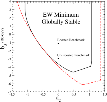
Figure 1: Absolute stability region for the EW vacuum in the $(a_{2},b_{3})$ plane for $b_{4}=1$, $c_{\theta}=0.812404$ and $m_{2}=270$ GeV (solid-black), $m_{2}=370$ GeV (dashed-red). The black dots correspond to the benchmark scenarios used in the analysis (see section IV).

III Current Constraints

For the process gluon-fusion mediated process $pp\rightarrow h_{2}\rightarrow h_{1}h_{1}$ of interest here, the magnitude of the cross section depends critically on the mixing angle $\theta$ through both the $h_{2}$ coupling to SM quarks and the triscalar coupling $\lambda_{211}$. The mixing angle is constrained by the current LHC results for properties of the SM Higgs boson. On the one hand, the cross section for $pp\rightarrow h_{1}$ is reduced compared to the one for a 125 GeV SM Higgs by a factor $c_{\theta}^{2}$ due to the singlet-doublet mixing. On the other, although the coupling of $h_{1}$ to its decay products is also universally suppressed by $c_{\theta}$, its decay branching ratios are the same as for a SM Higgs since no new decay channels are open. Consequently, the observation of the SM-like Higgs at the LHC can be used to set a lower bound on $c_{\theta}^{2}$ due to the associated signal suppression in SM Higgs decay channels. Recent global analyses of LHC Higgs measurements then yield $c_{\theta}^{2}>0.66$ at 0.95% C.L. Winslow13 ; ATLASCoup . From the analysis in Profumo:2007wc we observe that for mixing angles in this range and $m_{2}>2m_{1}$, the xSM can lead to a strong first order electroweak phase transition.

Global fits to electroweak precision data also imply constraints on the mixing angle and $m_{2}$. Although a reanalysis of these constraints goes beyond the scope of the present investigation, previous studies indicate that significant singlet-doublet mixing is disfavored for heavier $h_{2}$ Profumo:2007wc .

Another important constraint comes from ATLAS ATLASHeavyWW ; ATLASHeavyZZ and CMS CMSHeavy direct searches for heavy scalars decaying to $W\,W$ and $Z\,Z$. As the resulting constraints are dependent on the heavy scalar mass, we note that in the next section we will choose as benchmark scenarios for our analysis $m_{2}=270$ GeV and $m_{2}=370$ GeV. ATLAS searches in the $W\,W$ channel exclude $h_{2}$ at $95\,\%$ C.L. for $(\sigma\times\mathrm{Br})/(\sigma\times\mathrm{Br})_{\mathrm{SM}}\gtrsim 0.7$ for $m_{2}\sim 270$ GeV and $(\sigma\times\mathrm{Br})/(\sigma\times\mathrm{Br})_{\mathrm{SM}}\gtrsim 0.4$ for $m_{2}\sim 370$ GeV, while $Z\,Z$ searches exclude $h_{2}$ at $95\,\%$ C.L. for $(\sigma\times\mathrm{Br})/(\sigma\times\mathrm{Br})_{\mathrm{SM}}\gtrsim 0.25$ for $m_{h_{2}}\sim 270$ GeV and $(\sigma\times\mathrm{Br})/(\sigma\times\mathrm{Br})_{\mathrm{SM}}\gtrsim 0.3$ for $m_{h_{2}}\sim 370$ GeV. The bounds extracted from CMS searches are found to be similar. The production cross section for $h_{2}$ in the present case is given by $s_{\theta}^{2}\,\sigma_{\mathrm{SM}}$, and thus for $s_{\theta}^{2}\leq 0.34$ the constraints from $W\,W$ searches are satisfied, while a mild reduction in the branching fraction $h_{2}\rightarrow Z\,Z$ compared to the SM, due to the $h_{2}\rightarrow h_{1}\,h_{1}$ decay channel being available, suffices to satisfy also the constraints from $Z\,Z$ searches.

IV Resonant di-Higgs Production at the LHC

We now consider in detail resonant di-Higgs production at the LHC for $\sqrt{s}=14$ TeV. We focus on the gluon fusion production mechanism that is by far the dominant one for $m_{2}$ in the mass range of interest for the EWPT. The production mechanism is analogous to Higgs pair production in the SM via the trilinear Higgs self-coupling Dolan:2012rv , except that (a) the $s$-channel $gg\to h_{2}\to h_{1}h_{1}$ amplitude may be resonant in the present case (see also Dolan:2012ac ); and (b) the $ggh_{2}$ interaction will be reduced in strength by $c_{\theta}$.

Before discussing our rationale for focusing on the $b{\bar{b}}\tau^{+}\tau^{-}$ final state, it is useful to compare the expected magnitudes of the resonant and non-resonant di-Higgs production cross sections for the ranges of masses and couplings we consider below. The two most important contributions to the non-resonant cross section arise from the $gg\to h_{1}h_{1}$ amplitude involving the top quark box graph and from the $gg\to h_{1}^{\ast}\to h_{1}h_{1}$ process. The former will be reduced in strength from its SM value by $c^{2}_{\theta}$, while the latter will be reduced by $c_{\theta}\times\lambda_{111}/\lambda_{\mathrm{SM}}$. Taking $c^{2}_{\theta}=0.66$ and the SM di-Higgs production cross section from Dolan:2012rv for $\lambda_{111}=0$ we obtain $\sigma(pp\to h_{1}h_{1})_{\mathrm{non-res}}\approx 26$ fb, which lies well below our typical values for the resonant cross section: $\mathcal{O}(1)\,\mathrm{pb}$ for $m_{2}\lesssim 400$ GeV. Depending on the choices of the remaining independent parameters, the non-resonant $gg\to h_{1}^{\ast}\to h_{1}h_{1}$ process may interfere constructively with the box contribution, leading to as much as a factor of two increase in the total non-resonant cross section. The resulting cross section nevertheless lies well below the typical resonant production cross sections for the range of $m_{2}$ that we study here, so we may safely disregard the non-resonant $h_{1}h_{1}$ contribution in our analysis.

For the signal, we consider the $b\bar{b}\tau^{+}\tau^{-}$ final state since it has a sufficiently large branching ratio to yield a significant number of events with $\sim 100\,\,\mathrm{fb}^{-1}$ integrated luminosity yet does not contend with insurmountable backgrounds. For the final states with the largest branching ratio, $b\bar{b}b\bar{b}$ and $b{\bar{b}}W^{+}W^{-}$, the substantial backgrounds ($\buildrel>\over{{}_{\sim}}21$ pb and $\buildrel<\over{{}_{\sim}}900$ pb cross sections, respectively, Dolan:2012rv ) are challenging at best and may be insurmountable. In contrast, for the $b{\bar{b}}\tau^{+}\tau^{-}$ channel the potential $\buildrel<\over{{}_{\sim}}900$ pb $b{\bar{b}}W^{+}W^{-}$ background gets reduced to $\buildrel<\over{{}_{\sim}}20$ pb due to the small $W\rightarrow\ell\nu,\tau\nu$ branching fraction, as shown in studies of this channel in the context of SM di-Higgs production Another potentially promising search channel is the $b{\bar{b}}\gamma\gamma$ final state. An earlier analysis of this channel in the context of the real triplet extension of the SM FileviezPerez:2008bj indicates that discovery with $\sim 100$ fb^-1 of integrated luminosity would be possible using these final state when the triplet scalar pair production cross section is of order one picobarn. As indicated above, we defer an investigation of this channel to future work.

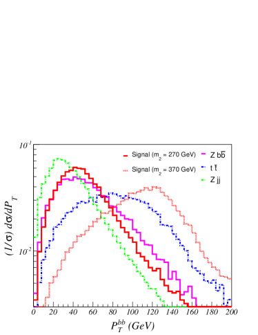
Figure 2: Normalized $|{\vec{P}}_{T}|$ distribution for the $b\bar{b}$ system, for both signal and the dominant backgrounds.

For the simulation of resonant di-Higgs production, we include both the $gg\to h_{2}\to h_{1}h_{1}$ and $gg\to h_{2}+j\to h_{1}h_{1}+j$ processes in order to improve the reliability of the kinematic distributions of the $h_{1}$ bosons and their decay products, even though we do not explicitly make use of the presence of this additional hard jet in our analysis. For the partonic gluon fusion process, we have implemented the xSM Lagrangian together with the scalar potential (II) in FeynRules Christensen:2008py ; Degrande:2011ua , including the $5$-dimensional gluon fusion effective operator $\mathcal{A}_{g}HG_{\mu\nu}^{a}G^{a\,\mu\nu}$ with the full LO form factor $\mathcal{A}_{g}$ that receives its leading contribution from the top quark triangle loop. Signal events are generated in MadGraph/MadEvent 5  Alwall:2011uj and subsequently interfaced to Pythia Sjostrand:2007gs for parton showering, jet matching and hadronization using the CTEQ611 parton luminosities Pumplin:2002vw set. The events are finally interfaced to PGS, which uses an anti-$k_{t}$ jet reconstruction algorithm. To set the overall normalization, we rescale our simulated K-factor $K=\sigma(pp\to h_{1}h_{1}X)_{\mathrm{NLO}}/\sigma(pp\to h_{1}h_{1}X)_{\mathrm{LO}}$ by the value computed in Ref. Dawson:1998py and updated in Ref. Baglio:2012np that takes into account the full set of NLO QCD corrections.

We perform our study for two benchmark parameter space points:

• Un-boosted Scenario: $m_{2}=270$ GeV, $c_{\theta}=0.812404$, $\lambda_{211}\,v=325$ GeV (with $a_{2}=0$, $b_{3}=-293$ GeV).

• Boosted Scenario: $m_{2}=370$ GeV, $c_{\theta}=0.812404$, $\lambda_{211}\,v=325$ GeV (with $a_{2}=0$, $b_{3}=-112$ GeV).

For case (a), the di-Higgs pair is produced nearly at rest in the $h_{2}$ rest frame, so the $p_{T}$ distribution for each $h_{1}$ is peaked well below 150 GeV, as illustrated in Fig. 2. There we show the $|{\vec{p}}_{T}|$ distribution of the $b{\bar{b}}$ pair produced by one of the decaying $h_{1}$ bosons along with the corresponding dominant backgrounds (see below). For this regime, the results obtained from the effective theory above are expected to agree qualitatively very well with those using the full 1-loop matrix element Dolan:2012rv . For case (b) the di-Higgs pair is boosted, with the $h_{1}$ $p_{T}$ distribution peaking near 130 GeV (see Fig.  2). In this regime, one approaches the limit of validity of the effective theory, so we do not consider heavier $m_{2}$. After taking int account NLO QCD corrections as discussed above, the corresponding inclusive di-Higgs production cross sections are 808 fb (420 fb) for the unboosted (boosted) scenarios.

IV.1 Analysis of $b\bar{b}\tau^{+}\tau^{-}$ Final States

Maximizing the sensitivity to the $b{\bar{b}}\tau^{+}\tau^{-}$ produced from $h_{2}\rightarrow h_{1}h_{1}$ decays entails reducing backgrounds generated by SM QCD and electroweak processes. A crucial step in this direction is the reconstruction of the invariant mass of the $b\bar{b}$ and $\tau^{+}\tau^{-}$ pairs that should individually reproduce the $h_{1}$ peak. The MMC technique Elagin:2010aw commonly used by the ATLAS and CMS collaborations Chatrchyan:2012vp ; Aad:2012mea to reconstruct the invariant mass of a $\tau^{+}\tau^{-}$ system from a decaying resonance relies on maximum likelihood methods that are not possible to implement in the present analysis. Alternatively, we use the collinear approximation Ellis:1987xu to reconstruct the di-tau invariant mass, which is used in experimental analyses of boosted resonances Aad:2012mea . This procedure consists of assuming that the invisible neutrinos from the $\tau$ decays are emitted collinear with the visible products of the decay. It is then possible to obtain the absolute value of the missing momentum in each $\tau$ decay $p^{\mathrm{mis}}_{1,2}$ using the missing energy vector $\vec{E}^{\mathrm{miss}}_{T}$ in the event and the kinematics of the visible decay products:

$$p^{\mathrm{mis}}_{1}=\frac{\mathrm{sin}(\phi^{\mathrm{vis}}_{2})E^{\mathrm{miss}}_{Tx}-\mathrm{cos}(\phi^{\mathrm{vis}}_{2})E^{\mathrm{miss}}_{Ty}}{\mathrm{sin}(\theta^{\mathrm{vis}}_{1})\,\mathrm{sin}(\phi^{\mathrm{vis}}_{2}-\phi^{\mathrm{vis}}_{1})}$$ (10)

$$p^{\mathrm{mis}}_{2}=\frac{\mathrm{cos}(\phi^{\mathrm{vis}}_{1})E^{\mathrm{miss}}_{Ty}-\mathrm{sin}(\phi^{\mathrm{vis}}_{1})E^{\mathrm{miss}}_{Tx}}{\mathrm{sin}(\theta^{\mathrm{vis}}_{2})\,\mathrm{sin}(\phi^{\mathrm{vis}}_{2}-\phi^{\mathrm{vis}}_{1})}$$ (11)

One then defines:

$$x_{1,2}=\frac{p^{\mathrm{vis}}_{1,2}}{p^{\mathrm{vis}}_{1,2}+p^{\mathrm{mis}}_{1,2}}$$ (12)

where $p^{\mathrm{vis}}$ is the absolute value of the momentum of the visible products in each $\tau$ decay. The invariant mass of the $\tau^{+}\tau^{-}$ pair is then obtained as $m_{\tau\tau}^{\mathrm{coll}}=m_{\tau\tau}^{\mathrm{vis}}/\sqrt{x_{1}\,x_{2}}$, with $m_{\tau\tau}^{\mathrm{vis}}$ being the invariant mass of the visible decay products of the $\tau^{+}\tau^{-}$ system.

The primary disadvantage of the collinear approximation (10)-(12) is that it is not well-defined when the two $\tau$’s from the decay of $h$ are emitted back-to-back in the transverse plane ($\left|\phi_{1}-\phi_{2}\right|\sim\pi$), which manifests itself in the divergence of $p^{\mathrm{mis}}_{1,2}$ as $\left|\phi_{1}-\phi_{2}\right|\rightarrow\pi$. Moreover, in this configuration, the transverse momenta of the two neutrinos will tend to cancel each other, generically resulting in little missing energy ${E}_{T}^{\mathrm{miss}}$, which also renders the collinear approximation inefficient.

Description	Rationale
$N_{b_{\mathrm{tag}}}=2$ , $N_{\ell}=2$	signal selection
$p_{T}^{\ell}>10$ GeV	lepton selection
$p_{T}^{b}>10$ GeV	$b$-jet selection
$\Delta R_{bb}>0.5$, $|y_{b}|<2.5$	$b$-jet selection
$\Delta R_{bb}>2.1$	$Zjj$, $Zb{\bar{b}}$, $t{\bar{t}}$ reductiona
$P_{T,b_{1}}>45\,\mathrm{GeV},\,P_{T,b_{2}}>30\,\mathrm{GeV}$	$Zjj$, $Zb{\bar{b}}$, $t{\bar{t}}$ reductionb
$90\,\mathrm{GeV}<m_{bb}<140\,\mathrm{GeV}$	$h_{1}$ mass reconstructionc
Collinear $x_{1},\,x_{2}$ Cuts	$m^{\mathrm{coll}}_{\tau\tau}$ reconstruction
$\Delta R_{\ell\ell}>2$	$t{\bar{t}}$ reductiond
$H_{T}^{\mathrm{lept}}<120\,\mathrm{GeV}$	$t{\bar{t}}$ reduction
$30\,\mathrm{GeV}<m_{\ell\ell}<75\,\mathrm{GeV}$	$Z$-peak veto
$30\,\mathrm{GeV}<m_{e\mu}<100\,\mathrm{GeV}$
$100\,\mathrm{GeV}<m^{\mathrm{coll}}_{\tau\tau}<150\,\mathrm{GeV}$	$h_{1}$ mass reconstruction
$E_{T}^{\mathrm{miss}}<50\,\mathrm{GeV}$	$t{\bar{t}}$ reductione
$230\,\mathrm{GeV}<m^{\mathrm{coll}}_{bb\tau\tau}<300\,\mathrm{GeV}$	$h_{2}$ mass reconstruction

Table 1: Event selection criteria and ordered cut flow for background reduction in the $b{\bar{b}}\tau_{\mathrm{lep}}\tau_{\mathrm{lep}}$ channel. See: ^aFig. 3, ^bFig. 5, ^cFig. 4, ^dFig. 6, and ^eFig. 7.

Imposing the collinear cut $0.1<x_{1},x_{2}<1$ eliminates events with a back-to-back configuration, so we use it when selecting events used for the reconstruction of the di-tau invariant mass, $m_{\tau\tau}^{\mathrm{coll}}$. For the single Higgs gluon fusion process $pp\rightarrow h\rightarrow\tau^{+}\tau^{-}$ the $\tau$ leptons are generically emitted nearly back-to-back since the Higgs is produced almost at rest in the transverse plane. The collinear approximation is more effective for single Higgs production in conjunction with a high-$p_{T}$ jet against which the di-tau pair recoils, thereby reducing the incidence of back-to-back $\tau$ pairs. For di-Higgs production, the $h_{1}$ decaying to the $b{\bar{b}}$ pair takes the place of the high $p_{T}$ jet, so we expect the use of the collinear approximation to be reasonably reliable in the case of our analysis (see also Ref. Aad:2012mea ).

The most relevant backgrounds for the analysis of $b\bar{b}\tau^{+}\tau^{-}$ final states are $Zb{\bar{b}}$, $Z+jets$ (with two jets mis-identified as $b$ quark objects) and $t{\bar{t}}$ production (the primary source of the large $b{\bar{b}}W^{+}W^{-}$ background indicated above). As we do not consider in the present analysis the possibility of jets faking hadronically decaying $\tau$ leptons, we disregard certain possible (albeit less important) backgrounds such as $b{\bar{b}}Wj$ and $b{\bar{b}}jj$. As with the signal, all background events are generated in MadGraph/MadEvent 5 and subsequently interfaced to Pythia and PGS. The various background cross-sections are normalized to their respective NLO values via enhancement $K$ factors: $K\simeq 1.4$ for $Zb{\bar{b}}$ Campbell:2005zv and $K\simeq 1.5$ for $t{\bar{t}}$ Mangano:1991jk ; Bevilacqua:2010qb (for $Zjj$, the NLO cross section is similar to the LO one for renormalization and factorization scales chosen as $\mu_{R}=\mu_{F}=M_{Z}$ Campbell:2003hd ). Following ATLAS_Tech , our detector simulation is normalized to a 70% b-tagging efficiency for b-quark jets with $|y|<2.5$ together with a 60% efficiency for identification of hadronic $\tau$’s.

	$h_{2}\rightarrow h_{1}h_{1}$		$t\bar{t}$		$Z\,b\bar{b}$	$Z\,jj$
	$b{\bar{b}}\tau_{\mathrm{lep}}\tau_{\mathrm{lep}}$	$b{\bar{b}}\ell\ell$	$b{\bar{b}}\ell\tau_{\mathrm{lep}}$	$b{\bar{b}}\tau_{\mathrm{lep}}\tau_{\mathrm{lep}}$	$b{\bar{b}}\ell\ell$ + $b{\bar{b}}\tau_{\mathrm{lep}}\tau_{\mathrm{lep}}$	$jj\ell\ell$ + $jj\tau_{\mathrm{lep}}\tau_{\mathrm{lep}}$
Event selection (see section V.B)	7.47	11209	4005	289	8028	1144
$\Delta R_{bb}>2.1$, $P_{T,b_{1}}>45$ GeV, $P_{T,b_{2}}>30$ GeV	4.46	5585	2013	145	2471	153
$h_{1}$-mass: $90$ GeV $<m_{bb}<140$ GeV	3.12	1073	405	30	880	47
Collinear $x_{1},\,x_{2}$ Cuts	2.34	438	164	14.1	248	18
$\Delta R_{\ell\ell}>2$, $H_{T}^{\mathrm{lept}}<120$ GeV	2.08	226	82	7.9	200	16.7
$30$ GeV $<m_{\ell\ell}\,(m_{e\mu})<75\,(100)$ GeV	1.86	136	49	5.7	11.6	0.95
$h_{1}$-mass: $100$ GeV $<m^{\mathrm{coll}}_{\tau\tau}<150$ GeV	1.05	32.5	11.4	1.63	3.24	0.24
$E_{T}^{\mathrm{miss}}<50$ GeV	0.89	10.5	3.37	0.56	3.03	0.23
$h_{2}$-mass: $230$ GeV $<m^{\mathrm{coll}}_{bb\tau\tau}<300$ GeV	0.81	1.19	0.39	0.12	0.86	0.09

Table 2: Event selection and background reduction for the $b{\bar{b}}\tau_{\mathrm{lep}}\tau_{\mathrm{lep}}$ channel in the un-boosted benchmark scenario. We show the NLO cross section (in $\mathrm{fb}$) for the signal $h_{2}\rightarrow h_{1}h_{1}\rightarrow b{\bar{b}}\tau_{\mathrm{lep}}\tau_{\mathrm{lep}}$ and the relevant backgrounds $t\bar{t}\rightarrow b{\bar{b}}\tau_{\mathrm{lep}}\tau_{\mathrm{lep}},\,b{\bar{b}}\ell\tau_{\mathrm{lep}},\,b{\bar{b}}\ell\ell$, $Z\,b\bar{b}\rightarrow b{\bar{b}}\tau_{\mathrm{lep}}\tau_{\mathrm{lep}},\,\,b{\bar{b}}\ell\ell$ and $Z\,jj\rightarrow jj\tau_{\mathrm{lep}}\tau_{\mathrm{lep}},\,\,jj\ell\ell$ after successive cuts. A 70% b-tagging efficiency is assumed, following ATLAS_Tech , together with a jet fake rate of 2% (slightly more conservative than that from ATLAS_Tech ).

	$h_{2}\rightarrow h_{1}h_{1}$		$t\bar{t}$		$Z\,b\bar{b}$	$Z\,jj$
	$b{\bar{b}}\tau_{\mathrm{lep}}\tau_{\mathrm{lep}}$	$b{\bar{b}}\ell\ell$	$b{\bar{b}}\ell\tau_{\mathrm{lep}}$	$b{\bar{b}}\tau_{\mathrm{lep}}\tau_{\mathrm{lep}}$	$b{\bar{b}}\ell\ell$ + $b{\bar{b}}\tau_{\mathrm{lep}}\tau_{\mathrm{lep}}$	$jj\ell\ell$ + $jj\tau_{\mathrm{lep}}\tau_{\mathrm{lep}}$
Event selection (see section V.B)	4.24	11209	4005	289	8028	1144
$\Delta R_{bb}<2.2$, $P_{T,b_{1}}>50$ GeV, $P_{T,b_{2}}>30$ GeV	2.38	3356	1202	85	1166	35
$h_{1}$-mass: $90$ GeV $<m_{bb}<140$ GeV	1.89	1396	512	36	452	12
$|\vec{P}^{bb}_{T}|>110$ GeV	1.35	719	264	19	208	4.9
Collinear $x_{1},\,x_{2}$ Cuts	1.09	293	107	8.8	58	1.86
$\Delta R_{\ell\ell}<2.3$, $H_{T}^{\mathrm{lept}}<120$ GeV	0.80	120	45	4.2	9	0.14
$30$ GeV $<m_{\ell\ell}\,(m_{e\mu})<75\,(100)$ GeV	0.70	85	30	2.45	1.51	0.019
$h_{1}$-mass: $100$ GeV $<m^{\mathrm{coll}}_{\tau\tau}<150$ GeV	0.60	30	11	0.96	0.24	0.003
$25$ GeV $<E_{T}^{\mathrm{miss}}<90$ GeV	0.42	18	6.2	0.60	0.18	0.003
$h_{2}$-mass: $330$ GeV $<m^{\mathrm{coll}}_{bb\tau\tau}<400$ GeV	0.32	3.25	1.08	0.11	0.025	$<$ 0.001

Table 3: Event selection and background reduction for the $b{\bar{b}}\tau_{\mathrm{lep}}\tau_{\mathrm{lep}}$ channel in the boosted benchmark scenario (same assumptions as in Table 2).

It is useful to organize the analysis according to the different $\tau$-decay modes, following roughly the treatment in Ref. Aad:2012mea . We, thus, consider $b{\bar{b}}$ plus (a) two leptonically decaying $\tau$s (“$\tau_{\mathrm{lep}}\tau_{\mathrm{lep}}$”); (b) one leptonically decaying and one hadronically decaying $\tau$ (“$\tau_{\mathrm{lep}}\tau_{\mathrm{had}}$”); and (c) two hadronically decay $\tau$s (“$\tau_{\mathrm{had}}\tau_{\mathrm{had}}$”). After $\tau$ identification and b-tagging, the NLO cross sections for the unboosted (boosted) case are: (a) $\tau_{\mathrm{lep}}\tau_{\mathrm{lep}}$: $10.58\,(5.75)\,\mathrm{fb}$; (b) $\tau_{\mathrm{lep}}\tau_{\mathrm{had}}$: $23.39\,(12.71)\,\mathrm{fb}$; and (c) $\tau_{\mathrm{had}}\tau_{\mathrm{had}}$: $12.90\,(7.01)\,\mathrm{fb}$ for a total cross section of $46.85\,(25.48)\,\mathrm{fb}$.

IV.2 Leptonic ($\tau_{\mathrm{lep}}\tau_{\mathrm{lep}}$) final states.

When the two $\tau$-leptons in the final state decay leptonically ($\tau_{\mathrm{lep}}\tau_{\mathrm{lep}}$), the relevant backgrounds are $t\bar{t}\rightarrow b{\bar{b}}\ell\ell\nu{\bar{\nu}}$, $t\bar{t}\rightarrow b{\bar{b}}\ell\tau_{\mathrm{lep}}\nu{\bar{\nu}}$, $t\bar{t}\rightarrow b{\bar{b}}\tau_{\mathrm{lep}}\tau_{\mathrm{lep}}\nu{\bar{\nu}}$, $Z\,b\bar{b}\rightarrow b{\bar{b}}\ell\ell$, $Z\,b\bar{b}\rightarrow b{\bar{b}}\tau_{\mathrm{lep}}\tau_{\mathrm{lep}}$, $Z\,jj\rightarrow jj\ell\ell$ and $Z\,jj\rightarrow jj\tau_{\mathrm{lep}}\tau_{\mathrm{lep}}$. A summary of our selection and background reduction cuts for the unboosted case appears in Table 1. For the boosted pair case as well as for the $\tau_{\mathrm{lep}}\tau_{\mathrm{had}}$ and $\tau_{\mathrm{had}}\tau_{\mathrm{had}}$ final states, we will subsequently discuss modifications of this basic set of cuts implemented in our analysis.

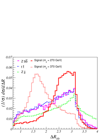
Figure 3: Normalized $\Delta R_{bb}$ distribution after event selection (before cuts) for signal and background (“$\tau_{\mathrm{lep}}\tau_{\mathrm{lep}}$”).

For the analysis of the $\tau_{\mathrm{lep}}\tau_{\mathrm{lep}}$ channel we select events containing exactly two $b$-tagged jets ($N_{b_{\mathrm{tag}}}=2$) and two isolated leptons ($N_{\ell}=2$). The cuts in $\Delta R_{bb}$, the $p_{T}$ of the two $b$-tagged jets and the invariant mass reconstructions for $b{\bar{b}}$, $\tau\tau$ and $b{\bar{b}}\tau\tau$ significantly reduce all backgrounds (see Figs. 3, 4, 5). In addition, the $Z$ backgrounds can be further suppressed by imposing cuts on the dilepton invariant mass, while $t{\bar{t}}$ is suppressed with a combination of cuts on $E_{T}^{\mathrm{miss}}$, the $\Delta R$ of the reconstructed di-tau pair (see Fig. 6), and the scalar sum of leptonic transverse momentum, $H_{T}^{\mathrm{lept}}$. We include all possible combinations of opposite sign leptons in our simulated samples ($ee$, $e\mu$ and $\mu\mu$). Further reduction of the $Z$ backgrounds could be achieved by considering only $e\mu$ pairs as in Ref. Aad:2012mea . Doing so in the present case, however, leads to a loss of signal without significantly improving the final $S/\sqrt{S+B}$.

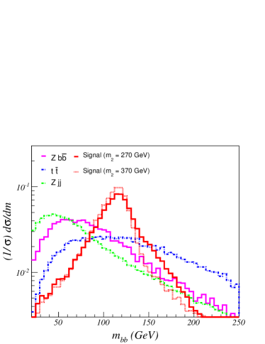
Figure 4: Normalized $m_{bb}$ distribution after event selection (before cuts) for signal and background (“$\tau_{\mathrm{lep}}\tau_{\mathrm{lep}}$”).

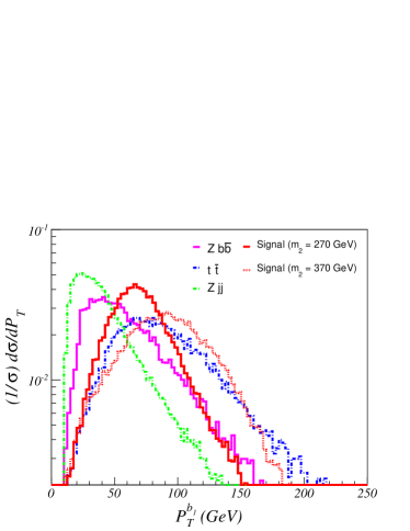
Figure 5: Normalized $P_{T,b_{1}}$ distribution after event selection (before cuts) for signal and background (“$\tau_{\mathrm{lep}}\tau_{\mathrm{lep}}$”).

For the boosted benchmark scenario, the $P_{T}$ of each $h_{1}$ will in general be substantially higher (see Fig. 2), and the $h_{1}$ decay products will tend to be more collimated. We accordingly modify our cuts by imposing an upper bound on both $\Delta R_{bb}$ and $\Delta R_{\ell\ell}$ together with an increase on the $P_{T,b_{1}}$ threshold, as suggested by Figs. 3, 5 and 6. While the $t{\bar{t}}$ distributions for $\Delta R_{bb}$ and $\Delta R_{\ell\ell}$ are relatively flat, those for the signal shift dramatically from the large to small $\Delta R$ range when going from the unboosted to the boosted regime (the $Zb{\bar{b}}$ and $Zjj$ backgrounds are reduced with separate cuts). In addition, we find further improvement in the $Zjj$ and $Zb{\bar{b}}$ background reduction by requiring a relatively large $|\vec{P}^{bb}_{T}|$ as is apparent from Fig. 2. The corresponding impact of the cut-flow on signal and background cross sections are given in Tables 2 and 3 for the unboosted and boosted scenarios, respectively.

In light of the results from Tables 2 and 3, for both $\tau$-leptons decaying leptonically a $S/\sqrt{S+B}\sim 5$ for the unboosted benchmark scenario can be achieved with $\sim 130-140\,\mathrm{fb}^{-1}$, while the boosted benchmark scenario requires $\gtrsim 1000\,\mathrm{fb}^{-1}$. The inability to efficiently reduce the $t{\bar{t}}$ background in the latter case is related to the greater amount of $E_{T}^{\mathrm{miss}}$ in the signal events (coming from the decay of the more boosted $\tau$-leptons) for the boosted scenario, which then renders the cut on $E_{T}^{\mathrm{miss}}$ relatively inefficient in suppressing the $t{\bar{t}}$ background, in contrast to the situation in the un-boosted scenario (see Fig. 7).

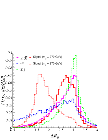
Figure 6: Normalized $\Delta R_{\ell\ell}$ distribution after event selection (before cuts) for signal and background (“$\tau_{\mathrm{lep}}\tau_{\mathrm{lep}}$”).

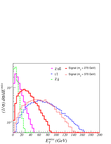
Figure 7: Normalized $E_{T}^{\mathrm{miss}}$ distribution after event selection (before cuts) for signal and background (“$\tau_{\mathrm{lep}}\tau_{\mathrm{lep}}$”)

IV.3 Semileptonic ($\tau_{\mathrm{lep}}\tau_{\mathrm{had}}$) final states.

	$h_{2}\rightarrow h_{1}h_{1}$		$t\bar{t}$		$Z\,b\bar{b}$	$Z\,jj$
	$b{\bar{b}}\tau_{\mathrm{lep}}\tau_{\mathrm{had}}$	$b{\bar{b}}\ell\tau_{\mathrm{had}}$		$b{\bar{b}}\tau_{\mathrm{lep}}\tau_{\mathrm{had}}$	$b{\bar{b}}\tau_{\mathrm{lep}}\tau_{\mathrm{had}}$	$jj\tau_{\mathrm{lep}}\tau_{\mathrm{had}}$
Event selection (see section V.C)	19.17	5249		762	601	98
$\Delta R_{bb}>2.1$, $P_{T,b_{1}}>45$ GeV, $P_{T,b_{2}}>30$ GeV	11.45	2639		384	188	10.8
$h_{1}$-mass: $90$ GeV $<m_{bb}<140$ GeV	8.00	531		80	69	3.68
Collinear $x_{1},\,x_{2}$ Cuts	4.81	209		36.4	41.6	2.41
$\Delta R_{\ell\tau}>2$	4.10	129		23.1	26.5	2.03
$m^{\ell}_{T}<30$ GeV	3.44	30.9		11.1	24.4	1.90
$h_{1}$-mass: $110$ GeV $<m^{\mathrm{coll}}_{\tau\tau}<150$ GeV	1.56	4.97		2.05	4.92	0.38
$E_{T}^{\mathrm{miss}}<50$ GeV	1.37	3.31		0.87	4.29	0.36
$h_{2}$-mass: $230$ GeV $<m^{\mathrm{coll}}_{bb\tau\tau}<300$ GeV	1.29	0.39		0.17	1.21	0.13

Table 4: Event selection and background reduction for the $b{\bar{b}}\tau_{\mathrm{lep}}\tau_{\mathrm{had}}$ channel in the un-boosted benchmark scenario. We show the NLO cross section (in $\mathrm{fb}$) for the signal $h_{2}\rightarrow h_{1}h_{1}\rightarrow b{\bar{b}}\tau_{\mathrm{lep}}\tau_{\mathrm{had}}$ and the relevant backgrounds $t\bar{t}\rightarrow b{\bar{b}}\tau_{\mathrm{lep}}\tau_{\mathrm{had}},\,b{\bar{b}}\ell\tau_{\mathrm{had}}$, $Z\,b\bar{b}\rightarrow b{\bar{b}}\tau_{\mathrm{lep}}\tau_{\mathrm{had}}$ and $Z\,jj\rightarrow jj\tau_{\mathrm{lep}}\tau_{\mathrm{had}}$ after successive cuts (same efficiency and face rate assumptions as in Table 2).

	$h_{2}\rightarrow h_{1}h_{1}$		$t\bar{t}$		$Z\,b\bar{b}$	$Z\,jj$
	$b{\bar{b}}\tau_{\mathrm{lep}}\tau_{\mathrm{had}}$	$b{\bar{b}}\ell\tau_{\mathrm{had}}$		$b{\bar{b}}\tau_{\mathrm{lep}}\tau_{\mathrm{had}}$	$b{\bar{b}}\tau_{\mathrm{lep}}\tau_{\mathrm{had}}$	$jj\tau_{\mathrm{lep}}\tau_{\mathrm{had}}$
Event selection (see section V.C)	10.73	5249		762	601	98
$\Delta R_{bb}<2.2$, $P_{T,b_{1}}>50$ GeV, $P_{T,b_{2}}>30$ GeV	6.02	1576		223	85	2.46
$h_{1}$-mass: $90$ GeV $<m_{bb}<140$ GeV	4.77	672		94	31.5	0.84
$|\vec{P}^{bb}_{T}|>110$ GeV	3.42	345		49	13.9	0.33
Collinear $x_{1},\,x_{2}$ Cuts	2.31	136		22.3	8.38	0.22
$\Delta R_{\ell\tau}<2.3$	1.71	68		11.1	4.31	0.055
$m^{\ell}_{T}<30$ GeV	1.46	18.4		5.64	4.02	0.051
$h_{1}$-mass: $110$ GeV $<m^{\mathrm{coll}}_{\tau\tau}<150$ GeV	1.05	4.2		1.26	0.30	0.003
$25$ GeV $<E_{T}^{\mathrm{miss}}<90$ GeV	0.76	2.93		0.75	0.23	0.002
$h_{2}$-mass: $330$ GeV $<m^{\mathrm{coll}}_{bb\tau\tau}<400$ GeV	0.63	0.60		0.15	0.026	$<$ 0.001

Table 5: Event selection and background reduction for the $b{\bar{b}}\tau_{\mathrm{lep}}\tau_{\mathrm{had}}$ channel in the boosted benchmark scenario (same efficiency and face rate assumptions as in Table 2).

For the $b{\bar{b}}\tau_{\mathrm{lep}}\tau_{\mathrm{had}}$ final state, we require exactly one isolated lepton and one hadronically decaying tau (“$\tau_{h}$”), where the latter is identified using the PGS detector simulator. The event selection criteria for this channel are given by: $N_{b_{\mathrm{tag}}}=2$, $N_{\ell}=1$, $N_{\tau_{h}}=1$ , $p_{T}^{\ell},p_{T}^{\tau}>10$ GeV, $|y_{b}|<2.5$, $\Delta R_{bb}>0.5$, $p_{T}^{b}>10$. The main backgrounds arise from $t{\bar{t}}$ with $b{\bar{b}}\ell\tau_{\mathrm{had}}\nu{\bar{\nu}}$ and $b{\bar{b}}\tau_{\mathrm{lep}}\tau_{\mathrm{had}}\nu{\bar{\nu}}$ produced in the $t$-quark decays, and $Zb{\bar{b}}$, $Zjj$ with $Z\to\tau_{\mathrm{lep}}\tau_{\mathrm{had}}$. The imposed cuts are similar to those applied to the $\tau_{\mathrm{lep}}\tau_{\mathrm{lep}}$ case, except for the di-lepton invariant mass cuts. Instead, to reduce backgrounds associated with $b{\bar{b}}WW$ events (largely dominated by $t{\bar{t}}$ production), we cut on the transverse mass of the lepton (see Fig. 8)

$$m^{\ell}_{T}=\sqrt{2p_{T}^{\ell}E_{T}^{\mathrm{miss}}(1-\cos\phi_{\ell,\mathrm{miss}})}<30\ \mathrm{GeV}$$ (13)

with $\phi_{\ell,\mathrm{miss}}$ being the azimuthal angle between the direction of missing energy and the lepton transverse momentum.

The corresponding impact of the cut-flow on signal and background cross sections are given in Tables 4 and 5 for the unboosted and boosted scenarios. As for the $\tau_{\mathrm{lep}}\tau_{\mathrm{lep}}$ channel, the various cuts allow one to greatly suppress the backgrounds and increase the signal significance. For the $\tau_{\mathrm{lep}}\tau_{\mathrm{had}}$ channel, since it is not possible to impose a Z-peak veto through a cut in the invariant mass of the lepton pair, we increase the lower end of the $m^{\mathrm{coll}}_{\tau\tau}$ invariant mass signal window (from $100$ GeV to $110$ GeV) in order to suppress $Zb{\bar{b}}$ and $Zjj$ backgrounds. The distributions for $m^{\mathrm{coll}}_{\tau\tau}$ and $m^{\mathrm{coll}}_{bb\tau\tau}$ in this channel are shown in Figs. 9 and 10.

From the results from Tables 4 and 5, we find that for the semileptonic channel a $S/\sqrt{S+B}\sim 5$ for the unboosted benchmark scenario can be obtained with $\sim 50\,\mathrm{fb}^{-1}$, while for the boosted benchmark scenario the required integrated luminosity is slightly higher, $\sim 90\,\mathrm{fb}^{-1}$. This channel therefore appears to be promising both for the boosted and unboosted regimes.

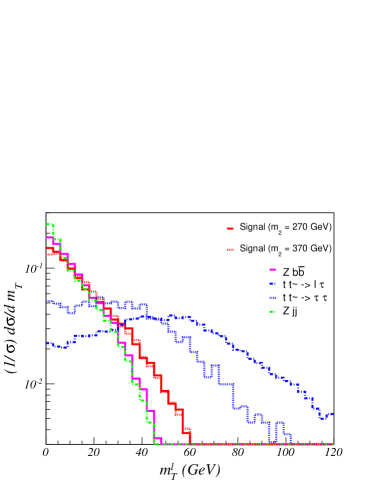
Figure 8: Normalized $m^{\ell}_{T}$ distribution for signal and background (“$\tau_{\mathrm{lep}}\tau_{\mathrm{had}}$”).

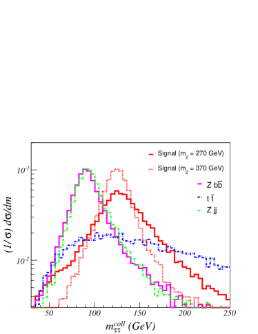
Figure 9: Normalized $m^{\mathrm{coll}}_{\tau\tau}$ distribution for $\tau^{+}\tau^{-}$ system in signal and background (“$\tau_{\mathrm{lep}}\tau_{\mathrm{had}}$”).

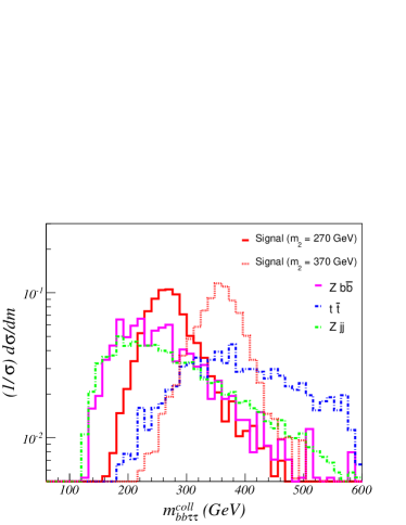
Figure 10: Normalized $m^{\mathrm{coll}}_{bb\tau\tau}$ distribution for signal and background (“$\tau_{\mathrm{lep}}\tau_{\mathrm{had}}$”).

IV.4 Hadronic ($\tau_{\mathrm{had}}\tau_{\mathrm{had}}$) final states.

The selection criteria for this channel are given by two hadronically-decaying $\tau$-leptons ($N_{\tau_{h}}=2$), exactly zero leptons ( $N_{\ell}=0$), and a similar set of kinematic requirements on the $\tau$ leptons and $b$-jets as in the other channels: $p_{T}^{\tau}>10$ GeV, $|y_{b}|<2.5$, $\Delta R_{bb}>0.5$, $p_{T}^{b}>10$. As compared to the semileptonic and leptonic channels, the backgrounds for the purely hadronic channel are smaller. The cut flows for the unboosted and boosted scenarios are given in Tables 6 and 7, respectively.

In light of the results from Tables 6 and 7, we obtain $S/\sqrt{S+B}\sim 5$ with $\sim 100\,\mathrm{fb}^{-1}$ in the hadronic channel for both the unboosted and boosted benchmark scenarios. While this channel appears to be promising both for both scenarios, we caution that we have not considered other pure QCD backgrounds, such as multijet or $b{\bar{b}}jj$ production, where the jets fake a hadronically decaying $\tau$ lepton. The reason is the difficulty of reliably quantifying the jet fake rate for these events, which while being under $5\%$, depends strongly on the characteristics of the jet ATLAS_Tech . While we do not expect this class of background contamination to be an impediment to signal observation in the $\tau_{\mathrm{had}}\tau_{\mathrm{had}}$ channel, we are less confident in our quantitative statements here than for the other final states.

	$h_{2}\rightarrow h_{1}h_{1}$	$t\bar{t}$	$Z\,b\bar{b}$	$Z\,jj$
	$b{\bar{b}}\tau_{\mathrm{had}}\tau_{\mathrm{had}}$	$b{\bar{b}}\tau_{\mathrm{had}}\tau_{\mathrm{had}}$	$b{\bar{b}}\tau_{\mathrm{had}}\tau_{\mathrm{had}}$	$jj\tau_{\mathrm{had}}\tau_{\mathrm{had}}$
Event selection (see section V.D)	12.31	509	411	67
$\Delta R_{bb}>2.1$, $P_{T,b_{1}}>45$ GeV, $P_{T,b_{2}}>30$ GeV	7.35	256	128	7.39
$h_{1}$-mass: $90$ GeV $<m_{bb}<140$ GeV	5.14	53	47	2.52
Collinear $x_{1},\,x_{2}$ Cuts	2.57	22.8	24.5	1.42
$\Delta R_{\tau\tau}>2$	2.04	12.4	15.8	1.19
$h_{1}$-mass: $110$ GeV $<m^{\mathrm{coll}}_{\tau\tau}<150$ GeV	0.82	1.79	3.75	0.27
$E_{T}^{\mathrm{miss}}<50$ GeV	0.75	0.60	3.39	0.26
$h_{2}$-mass: $230$ GeV $<m^{\mathrm{coll}}_{bb\tau\tau}<300$ GeV	0.72	0.08	1.03	0.11

Table 6: Event selection and background reduction for the $b{\bar{b}}\tau_{\mathrm{had}}\tau_{\mathrm{had}}$ channel in the unboosted benchmark scenario. We show the NLO cross section (in $\mathrm{fb}$) for the signal $h_{2}\rightarrow h_{1}h_{1}\rightarrow b{\bar{b}}\tau_{\mathrm{had}}\tau_{\mathrm{had}}$ and the relevant backgrounds $t\bar{t}\rightarrow b{\bar{b}}\tau_{\mathrm{had}}\tau_{\mathrm{had}}$, $Z\,b\bar{b}\rightarrow b{\bar{b}}\tau_{\mathrm{had}}\tau_{\mathrm{had}}$ and $Z\,jj\rightarrow jj\tau_{\mathrm{had}}\tau_{\mathrm{had}}$ after successive cuts (same efficiency and face rate assumptions as in Table 2).

	$h_{2}\rightarrow h_{1}h_{1}$	$t\bar{t}$	$Z\,b\bar{b}$	$Z\,jj$
	$b{\bar{b}}\tau_{\mathrm{had}}\tau_{\mathrm{had}}$	$b{\bar{b}}\tau_{\mathrm{had}}\tau_{\mathrm{had}}$	$b{\bar{b}}\tau_{\mathrm{had}}\tau_{\mathrm{had}}$	$jj\tau_{\mathrm{had}}\tau_{\mathrm{had}}$
Event selection (see section V.D)	6.71	509	411	67
$\Delta R_{bb}<2.2$, $P_{T,b_{1}}>50$ GeV, $P_{T,b_{2}}>30$ GeV	3.77	149	58	1.68
$h_{1}$-mass: $90$ GeV $<m_{bb}<140$ GeV	2.99	63	21.6	0.57
$|\vec{P}^{bb}_{T}|>110$ GeV	2.14	32.5	9.5	0.23
Collinear $x_{1},\,x_{2}$ Cuts	1.27	13.9	4.95	0.13
$\Delta R_{\tau\tau}<2.3$	0.92	8.1	2.51	0.034
$h_{1}$-mass: $110$ GeV $<m^{\mathrm{coll}}_{\tau\tau}<150$ GeV	0.64	1.91	0.26	0.002
$25$ GeV $<E_{T}^{\mathrm{miss}}<90$ GeV	0.47	0.98	0.19	0.001
$h_{2}$-mass: $330$ GeV $<m^{\mathrm{coll}}_{bb\tau\tau}<400$ GeV	0.39	0.23	0.03	$<$ 0.001

Table 7: Event selection and background reduction for the $b{\bar{b}}\tau_{\mathrm{had}}\tau_{\mathrm{had}}$ channel in the boosted benchmark scenario (same efficiency and face rate assumptions as in Table 2).

V Discussion and Outlook

Uncovering the full structure of the SM scalar sector and its possible extensions will be a central task for the LHC in the coming years. The results will have important implications not only for our understanding of the mechanism of electroweak symmetry-breaking but also for the origin of visible matter and the nature of dark matter. Extensions of the SM scalar sector that address one or both of these open questions may yield distinctive signatures at the LHC associated with either modifications of the SM Higgs boson properties and/or the existence of new states.

In this study, we have considered one class of Higgs portal scalar sector extensions containing a singlet scalar that can mix with the neutral component of the SU(2)_L doublet leading to two neutral states $h_{1,2}$. This xSM scenario can give rise to a strong first order electroweak phase transition as needed for electroweak baryogenesis; it maps direction onto the NMSSM in the decoupling limit; and it serves as a simple paradigm for mixed state signatures in Higgs portal scenarios that contain other SU(2)_L representations. Considering resonant di-Higgs production $pp\to h_{2}\to h_{1}h_{1}$, we have shown that a search for the $b{\bar{b}}\tau^{+}\tau^{-}$ final state could lead to discovery of this scenario with $\sim 100$ fb^-1 integrated luminosity for regions of the model parameter space of interest to cosmology. The most promising mode appears to involve one leptonically-decay and one hadronically-decaying $\tau$ lepton, though for $m_{2}$ close to $2m_{1}$ the purely leptonic decay modes of the $\tau$’s could also yield discovery as well. For purely hadronically-decay $\tau$ leptons, the significance obtained from our analysis looks promising, though a more refined study of the rate for jets faking hadronically decaying $\tau$’s would give one more confidence in the prospects for this mode.

The study of other final states formed from combinations of SM Higgs decay products, as suggested by the work of Ref. Liu:2013woa that appeared as we were completing this paper, would be a natural next step. Although we disagree with the quantitative results in that study (a preliminary application of their basic cuts to the $b{\bar{b}}\tau^{+}\tau^{-}$ final state yields $S/B\sim 1$ rather than the $\sim 200$ as these authors find), we concur that a detailed analysis of other novel states associated with resonant di-Higgs production would be a worthwhile effort.

Acknowledgements

J.M.N. thanks Veronica Sanz for very useful discussions. MJRM thanks B. Brau, C. Dallapiccola, and S. Willocq for helpful discussions and comments on the manuscript. Both authors thank H. Guo, T. Peng, and H. Patel for generating background event samples. J.M.N. is supported by the Science Technology and Facilities Council (STFC) under grant No. ST/J000477/1. MJRM was supported in part by U.S. Department of Energy contract DE-FG02-08ER41531 and the Wisconsin Alumni Research Foundation. The authors also thank the Excellence Cluster Universe at the Technical University of Munich, where a portion of this work was carried out.

References

- (1) A. Djouadi, W. Kilian, M. Muhlleitner, and P. Zerwas, Eur.Phys.J. C10, 45 (1999), hep-ph/9904287.
- (2) U. Baur, T. Plehn, and D. L. Rainwater, Phys.Rev. D67, 033003 (2003), hep-ph/0211224.
- (3) U. Baur, T. Plehn, and D. L. Rainwater, Phys.Rev. D68, 033001 (2003), hep-ph/0304015.
- (4) U. Baur, T. Plehn, and D. L. Rainwater, Phys.Rev. D69, 053004 (2004), hep-ph/0310056.
- (5) M. J. Dolan, C. Englert, and M. Spannowsky, JHEP 1210, 112 (2012), 1206.5001.
- (6) A. Papaefstathiou, L. L. Yang, and J. Zurita, Phys.Rev. D87, 011301 (2013), 1209.1489.
- (7) F. Goertz, A. Papaefstathiou, L. L. Yang, and J. Zurita, JHEP 1306, 016 (2013), 1301.3492.
- (8) A. J. Barr, M. J. Dolan, C. Englert, and M. Spannowsky, (2013), 1309.6318.
- (9) D. E. Morrissey and M. J. Ramsey-Musolf, New J.Phys. 14, 125003 (2012), 1206.2942.
- (10) M. J. Dolan, C. Englert, and M. Spannowsky, Phys.Rev. D87, 055002 (2013), 1210.8166.
- (11) S. Profumo, M. J. Ramsey-Musolf, and G. Shaughnessy, JHEP 0708, 010 (2007), 0705.2425.
- (12) J. R. Espinosa, T. Konstandin, and F. Riva, Nucl.Phys. B854, 592 (2012), 1107.5441.
- (13) U. Ellwanger, C. Hugonie, and A. M. Teixeira, Phys.Rept. 496, 1 (2010), 0910.1785.
- (14) J. Liu, X.-P. Wang, and S.-h. Zhu, (2013), 1310.3634.
- (15) D. O’Connell, M. J. Ramsey-Musolf, and M. B. Wise, Phys.Rev. D75, 037701 (2007), hep-ph/0611014.
- (16) J. McDonald, Phys.Rev. D50, 3637 (1994), hep-ph/0702143.
- (17) C. Burgess, M. Pospelov, and T. ter Veldhuis, Nucl.Phys. B619, 709 (2001), hep-ph/0011335.
- (18) V. Barger, P. Langacker, M. McCaskey, M. Ramsey-Musolf, and G. Shaughnessy, Phys.Rev. D79, 015018 (2009), 0811.0393.
- (19) M. Gonderinger, H. Lim, and M. J. Ramsey-Musolf, Phys.Rev. D86, 043511 (2012), 1202.1316.
- (20) J. R. Espinosa, C. Grojean, V. Sanz, and M. Trott, JHEP 1212, 077 (2012), 1207.7355.
- (21) R. Barbieri, D. Buttazzo, K. Kannike, F. Sala, and A. Tesi, Phys.Rev. D87, 115018 (2013), 1304.3670.
- (22) G. Belanger, B. Dumont, U. Ellwanger, J. Gunion, and S. Kraml, (2013), 1306.2941.
- (23) U. Ellwanger, JHEP 1308, 077 (2013), 1306.5541.
- (24) J. Cao, Z. Heng, L. Shang, P. Wan, and J. M. Yang, JHEP 1304, 134 (2013), 1301.6437.
- (25) Z. Kang, J. Li, T. Li, D. Liu, and J. Shu, Phys.Rev. D88, 015006 (2013), 1301.0453.
- (26) V. Barger, P. Langacker, M. McCaskey, M. J. Ramsey-Musolf, and G. Shaughnessy, Phys.Rev. D77, 035005 (2008), 0706.4311.
- (27) p. c. P. Winslow.
- (28) ATLAS Collaboration, (2013), ATLAS-Conf-2013-034.
- (29) ATLAS Collaboration, (2013), ATLAS-Conf-2013-067.
- (30) ATLAS Collaboration, (2013), ATLAS-Conf-2013-013.
- (31) CMS Collaboration, CMS-HIG-12-034, 1304.0213.
- (32) M. Gouzevitch et al., JHEP 1307, 148 (2013), 1303.6636.
- (33) P. Fileviez Perez, H. H. Patel, M. Ramsey-Musolf, and K. Wang, Phys.Rev. D79, 055024 (2009), 0811.3957.
- (34) N. D. Christensen and C. Duhr, Comput.Phys.Commun. 180, 1614 (2009), 0806.4194.
- (35) C. Degrande et al., Comput.Phys.Commun. 183, 1201 (2012), 1108.2040.
- (36) J. Alwall, M. Herquet, F. Maltoni, O. Mattelaer, and T. Stelzer, JHEP 1106, 128 (2011), 1106.0522.
- (37) T. Sjostrand, S. Mrenna, and P. Z. Skands, Comput.Phys.Commun. 178, 852 (2008), 0710.3820.
- (38) J. Pumplin et al., JHEP 0207, 012 (2002), hep-ph/0201195.
- (39) S. Dawson, S. Dittmaier, and M. Spira, Phys.Rev. D58, 115012 (1998), hep-ph/9805244.
- (40) J. Baglio et al., JHEP 1304, 151 (2013), 1212.5581.
- (41) A. Elagin, P. Murat, A. Pranko, and A. Safonov, Nucl.Instrum.Meth. A654, 481 (2011), 1012.4686.
- (42) CMS Collaboration, S. Chatrchyan et al., Phys.Lett. B713, 68 (2012), 1202.4083.
- (43) ATLAS Collaboration, G. Aad et al., JHEP 1209, 070 (2012), 1206.5971.
- (44) R. K. Ellis, I. Hinchliffe, M. Soldate, and J. van der Bij, Nucl.Phys. B297, 221 (1988).
- (45) J. M. Campbell, R. K. Ellis, F. Maltoni, and S. Willenbrock, Phys.Rev. D73, 054007 (2006), hep-ph/0510362.
- (46) M. L. Mangano, P. Nason, and G. Ridolfi, Nucl.Phys. B373, 295 (1992).
- (47) G. Bevilacqua, M. Czakon, A. van Hameren, C. G. Papadopoulos, and M. Worek, JHEP 1102, 083 (2011), 1012.4230.
- (48) J. M. Campbell, R. K. Ellis, and D. L. Rainwater, Phys.Rev. D68, 094021 (2003), hep-ph/0308195.
- (49) ATLAS Collaboration, (2013), Tech. Rept. ATL-PHYS-PUB-2013-004.