Buckets of Higgs and Tops
Abstract
We show that associated production of a Higgs with a top pair can be observed in purely hadronic decays. Reconstructing the top quarks in the form of jet buckets allows us to control QCD backgrounds as well as signal combinatorics. The background can be measured from side bands in the reconstructed Higgs mass. We back up our claims with a detailed study of the QCD event simulation, both for the signal and for the backgrounds.
I Introduction
Measuring the couplings of the recently discovered Higgs boson higgs_theo ; higgs_ex to the Standard Model fermions is a critical part of the investigation of the electroweak symmetry breaking mechanism at the LHC sfitter . The Standard Model coupling to the top quark is expected to be of order unity, making it a prime target for studying the effects of many different new physics models in and beyond the Higgs sector bsm_review . Together with the Higgs self coupling it dominates the extrapolation of weak–scale Higgs physics to more fundamental energy scales lecture . Measuring this parameter will uniquely probe extensions of the Higgs sector at the weak scale sfitter as well as at high scales.
However, with a production cross section of only at the 13 TeV LHC, measurements based on the channel are extremely difficult. Search strategies in the fully leptonic and semi-leptonic decay channels for the top have been suggested in combination with Higgs decays to tth_bb , tth_tautau , and tth_ww . These are challenging through a combination of combinatoric backgrounds, missing control regions, large QCD uncertainties on the backgrounds, and low rate. Typical luminosities required for a signal might well be in the 100 fb-1 range for 13 TeV collider energy, with a signal–to–background ratio well below 1:1.
In this paper we provide a feasibility study for the fully hadronic channel of production, i.e. a final state consisting of four -jets plus up to four un-tagged jets. This channel has not been studied yet. In fact, there exist only a few analyses targeting Higgs or new physics searches in purely hadronic channels without missing energy or leptons, most notably some recent top pair resonance tt_resonance ; buckets and sgluon searches steffen . However, the fully hadronic decay channel of has two possible advantages over the leptonic decay modes. First, hadronic decays of both the tops and the Higgs have the highest branching ratios of any decay mode. Second, without neutrinos and their missing momenta, a full reconstruction of the final state is possible, which allows for discrimination of signal and background and provides the best testing ground in the presence of possible experimental anomalies. In addition, this eight–parton final state has the highest jet multiplicity of any widely-considered Standard Model process at the LHC. Demonstrating our ability to understand and use such events is an important benchmark in our study of Standard Model physics at the LHC.
We separate the signal events from the large QCD background via a two-step process. For four -jet events, we first apply global acceptance cuts, giving us an enriched sample of signal events. We then reconstruct the tops using the “bucket algorithm” buckets , which closes the gap between kinematic top reconstruction at threshold and proper top taggers seymour ; tagger_review by targeting slightly boosted top quarks, with
| (1) |
The algorithm identifies the two top quarks in the event by permuting over jet assignments to three buckets, minimizing a distance metric on two of those buckets between the invariant mass of the jets in the buckets and the mass of the top. The remaining event contains two -jets, which allow us to reconstruct the Higgs decay with a probability above 60%.
It should be noted that the results in this paper deliberately only rely on a simple cut–and–count method. It allows us to identify many opportunities for data–driven side band calibration of the backgrounds, which is crucial to such high–multiplicity searches. As the top-reconstruction technique provides a good approximation of the momenta of all the particles in the original event, more sophisticated techniques can be used to improve rejection of background and signal selection.
In the next section, we study the major backgrounds to the search, including some global background rejection cuts. The bucket algorithm is introduced in Section III, where we also give a detailed estimate of the analysis performance. A detailed discussion of the QCD backgrounds and their simulation are included in Appendix A. Finally, in Appendix B we show the metrics for the top reconstruction.
II Multi-jet backgrounds and global cuts
Our analysis aims to extract the fully hadronic final state of production with the decay . For a Higgs mass of 125 GeV we assume the Standard Model branching ratio to the final state of 57.7% decay ; xs_group . We will require four -tagged jets in the final state, no leptons, and at least two un-tagged hard jets. We assume jet-based triggers for hard multi-jet events, similar to all–hadronic searches tt_resonance . The main four- backgrounds, ordered by relevance, are
| (2) |
The corresponding fake- channels are strongly suppressed if the experiments reach a 70% -tagging efficiency with 1% mis-tagging probability for light-flavor and gluon jets. We estimate the rate of the mis-tagged multi-jet background to be contribute to the actual rate at the 10% level, i.e. below the quoted uncertainties in the simulations of the primary background. Similarly, we can ignore the pure QCD events with four mis-tags.
For our event simulation we rely on Alpgen alpgen and Madgraph madgraph , both with a Pythia parton shower pythia , as well as on Sherpa sherpa . For the signal our main event sample includes zero and one hard extra jet merged in the Ckkw scheme ckkw in Sherpa. In Appendix A we compare the Sherpa results with the Madgraph simulation of plus up to one hard jet merged in the Mlm scheme mlm . We confirm that the sensitivity to simulation and QCD issues is minimal. Similarly, for the background, our main sample of events is produced by Sherpa and includes up to one hard QCD jet. A comparison with Alpgen samples in Appendix A again shows negligible dependence on the simulation techniques. We normalize the merged event samples to the NLO results of 504 fb for the signal tth_nlo ; xs_group and 1037 fb after generator cuts for the background ttbb_nlo . The background from Alpgen is small compared to the primary and backgrounds, with a cross section of at maximum 5% of the signal. As a result, it does not require an extensive study of the theoretical and simulation uncertainties, and will not be considered in detail.
The critical background for the hadronic signal with decays is the QCD process jets. Before any selection cuts, its total rate completely overwhelms the signal, with a cross section of 400 pb estimated by Alpgen after pre-selection cuts. However, as any QCD process it is dominated by soft and un-tagged jets with an additional enhancement from the gluon splitting . To extract our signal we will require four hard, well separated -tagged jets. We simulate these background events both in Alpgen and Sherpa with a hard process of (at least) four -jets.
As we will see in Section III, our bucket reconstruction of two tops and the Higgs will require at least two additional hard un-tagged jets. Therefore, our central background simulation is defined by the hard process plus parton shower in Alpgen, which results in a cross section of 2128 fb after pre-selection cuts. To ensure that our analysis is stable with respect to QCD uncertainties, we also simulate the background with Sherpa as plus zero and one matrix element jet merged (+0/1j). The computational expense of two jet merging is prohibitive here, and so is not included. However, to have a measure for the underlying theory uncertainties, we vary the renormalization and factorization scales in the Sherpa simulation by a factor 1/2 to 2 around the central scale, to ensure that our conclusions hold independent of these choices. We carefully compare our two background estimates in Appendix A, providing detailed information on kinematic distributions and the different simulation tools and hard processes.111We would like to thank the referees and the editor of Ref. buckets for strongly supporting this kind of analysis and then allowing us to postpone it to this paper. There, we test a couple of important assumptions underlying our analysis. First, we demonstrate that the bucket analysis allows only background events with at least two hard un-tagged jets in our signal region. For this region the Alpgen estimate of the rate is the appropriate and conservative choice. In addition, we demonstrate that our analysis is not too sensitive to describing the second un-tagged jet by either the hard matrix element (as in the Alpgen) or by the parton shower (as in Sherpa). Finally, the full merged +jets simulation would allow access to excellent control regions in the side band of the number of un-tagged jets, once these kinds of distributions are systematically evaluated by ATLAS and CMS jet_scaling .
Understanding the kinematics of the background and reducing it using global kinematic cuts will be the central topic of this section. In the next section, we will find that several of these kinematic cuts can be replaced with the requirement of top reconstruction, which allows for an increased purity of signal over background. In the actual buckets analysis in Section III, we only quote the Alpgen results for the background.
Compared to the signal rate, the raw QCD background (primarily jets) is overwhelmingly large, and so we must apply selection cuts before the top-finding bucket algorithm can be employed. First, we require all events to have four -tagged jets. These -jets must be central and widely separated, to avoid the phase space regions with enhanced splitting, with
| (3) |
In addition, we require at least two hard non- jets with
| (4) |
These naive acceptance cuts are very inefficient, for example when compared to sub-jet methods. However, the aim of this paper is to show that the purely hadronic process can be studied at the LHC, so we need to ensure that the pure QCD backgrounds can be reliably removed. Moreover, four individual -tags cannot be treated as statistically independent unless we at least assume very widely separated -jets. This necessitates the harsh cuts in this proof–of–concept analysis.
| After acceptance Eqs.(3) and (4) | 1.197 | 8.363 | 54.420 | 0.019 |
|---|---|---|---|---|
| After global cuts Eq. (6) | 0.134 | 0.558 | 2.734 | 0.041 |
| Mass window GeV | ||||
| closest | 0.096 | 0.299 | 1.577 | 0.051 |
| hard | 0.017 | 0.031 | 0.226 | 0.065 |
| soft | 0.060 | 0.173 | 0.893 | 0.056 |
| min | 0.071 | 0.246 | 1.143 | 0.051 |
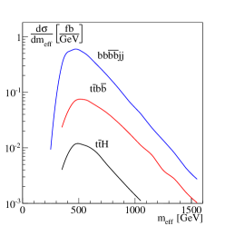
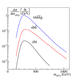
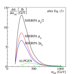
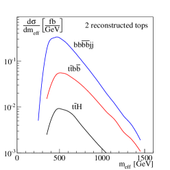
In the first line of Table 1 we show the cross sections for the signal and two primary backgrounds at the 13 TeV LHC, after acceptance cuts. The contribution is sub-percent level, and so not shown. At this stage the +jets cross section is still significantly larger than the signal, so an additional set of cuts is required. Once we introduce the top reconstruction technique, such cuts are not necessary, but it will be instructive to compare our later results to simple global cuts. We consider two global variables: the effective mass calculated by summing the scalar jet over all jets, including those with -tags, and its counterpart where the sum runs only over the four -tagged jets,
| (5) |
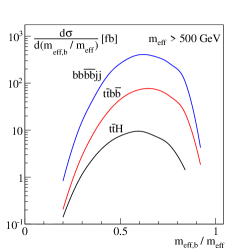
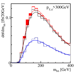
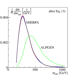
Both of these observables will be sensitive to the kinematics of the multi-jet system. In Figure 1 we show the distributions for both signal and backgrounds, normalized to the event rates after the cuts of Eqs.(3) and (4). At this point, the signal–to–background ratio is around 1:50. As we will discuss in Appendix A, the fact that the distributions of the signal and the backgrounds show a similar behavior is because our Alpgen simulation requires two hard un-tagged jets. In other words, the background simulation shown in Figure 1 anticipates the fact that we will only be interested in a reliable prediction of those background events which are kinematically similar to the signal. The right panel of Figure 1 shows that after requiring GeV both and have similar shapes for signal and background.
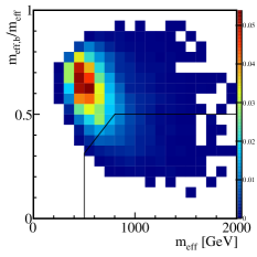
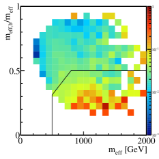
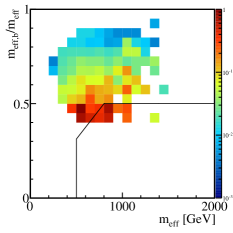
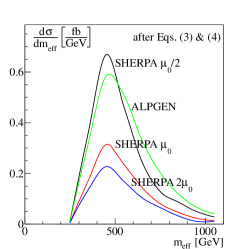
It is more efficient to consider the 2-dimensional plane of the two effective mass variables defined in Eq.(5). In Figure 2, we plot these distributions for the signal and the ratios of signal–to–background against the primary (jets) for both Alpgen and Sherpa simulations. As can be seen, the Sherpa simulation has many fewer events in the high tail compared to the Alpgen simulation, as expected due to the acceptance cut. The Sherpa simulation only generates up to one light-flavor or gluon jet from the hard matrix element, but the acceptance cuts require at least two hard un-tagged jets per event. As argued in Appendix A we use the jets sample from Alpgen for a more conservative background estimate. In this proof–of–concept paper, we make the crude requirements that
| (6) |
This set of cuts brings the background rate to a manageable level, without a detailed analysis of the top and Higgs kinematics. For the specific background modeling with Alpgen we arrive at , as quoted in Table 1.
From this point on, we are interested in identifying an excess of events that contain two -jets which are clearly identified with the Higgs boson decay. This is complicated by the combinatorial background of picking the correct two -jets out of the four in the event. First, we consider naive set of selection criteria for the two -jets which have to lie in the Higgs mass window in Table 1. We show that selecting the two -jets closest in mass to GeV, the two -jets with the softest , the two hardest, and the two -jets with the minimum invariant mass are all methods that fail to sufficiently increase signal over background.
Clearly, a better solution to the reconstruction of the top and Higgs decay products and the combinatorics associated with this assignment is needed. We therefore turn to the bucket reconstruction buckets to rebuild the two top quarks in the event, using those events that have passed our initial selection criteria described by Eqs.(3) and (4). This tags the two -jets that come from the tops with a good degree of accuracy, identifying the Higgs decay products by exclusion. With this method of identifying the correct -jets, the global cuts on variables do not improve the ratio, and so we do not continue to apply the cuts of Eq.(6). This simple algorithm is not meant to replace a full experimental likelihood analysis, but it shows that after simple kinematic cuts a purely hadronic analysis can be a realistic possibility.
III Top buckets
Following the arguments in the last section and the corresponding Appendix A it should be possible to devise an analysis of the hadronic top and Higgs kinematics to reduce the backgrounds to a manageable level. Aside from the irreducible background we need to extract the signal from the huge multi-jet background. A more specific analysis of the multi-jet final state should be able to do better than the already promising global effective mass cuts in Eq.(6). The key concern will be the signal efficiency, because of the limited rate. For this reason, we choose the bucket reconstruction buckets , which allows us to keep a larger fraction of signal events while removing significant parts of the background phase space identified by the global cuts analysis. The technical challenge is tracking the definition of the signal region and the corresponding background simulation.
After applying the jet-level selection cuts in the previous section, Eqs.(3) and (4), we have a sample of events with four -jets and additional extra jets. Of these four -jets, two are presumed to come from the Higgs decay, and two from top decays. Without knowledge of the top decays, various Higgs reconstruction schemes could be tried. As discussed in the previous section, one could take the two -jets with the highest or lowest , the combination of -jets with invariant mass that is closest to 125 GeV, the combination with the minimum invariant mass, or some other set based on simple jet kinematics. Taking the combination with the invariant mass closest to that of the Higgs in particular runs into a combinatorial problem: in both signal and background, one can often find two -jets with invariant mass near that of the Higgs without the jets involved having originated with the Higgs. This shapes the background to look like signal. The multi- combinatorics are the reason that the ATLAS search in the early phase of LHC running was largely abandoned cammin .
We can improve this situation if we find a better way to identify the -jets that come from the Higgs. We approach this problem by first identifying the decay products of the tops, using the top bucket algorithm. The idea behind this algorithm is very simple and straightforward: we divide all jets in every event into three buckets. Two of the buckets correspond to the hadronic tops, while the third bucket consists of all jets in the event that cannot be associated with a top. In the original formulation of the algorithm buckets this last bucket was identified with initial state radiation (ISR). In the current analysis, this ISR bucket will contain two -jets, which can — by exclusion — be identified as the decay products of the Higgs.
We start by seeding each of the two top buckets with a -jet. We permute over all possible assignments of -jets as top bucket seeds. We then cycle through every possible assignment of non--tagged jets to the three buckets, requiring at least one non-tagged jet in each of the top buckets. We use the distance metric
| (7) |
where is the top mass and the sum runs over all jets (including the -jet) in the bucket . We select the jet assignment that minimizes the distance measure , where is a factor chosen to stabilize the jet grouping. For this analysis, we choose , which essentially decouples the second bucket from the metric. Thus, bucket is the bucket with invariant mass closest to the top. After this construction, we have two buckets and , with two or three jets, including the seed -jet. Rarely, we find a bucket containing four or more jets, in which case we merge to three jets using the Cambridge/Aachen algorithm ca_algo .
To remove background events that do not contain real tops, we require the invariant masses of the two top buckets to lie in the window
| (8) |
Next, we require both and buckets to contain a hadronically decaying boson candidate. We define a mass ratio cut, as in the HEPTopTagger heptop_stops ,
| (9) |
for at least one combination of the non--jets (denoted and ) in the bucket . Buckets with only one -tagged and one non-tagged jet by construction cannot satisfy Eq.(9). We can therefore classify events in one of three categories:
-
•
(,): both top buckets have candidates as defined by Eq.(9),
-
•
(,) or (,): only the first or second top bucket has a candidate,
-
•
(,): neither top bucket has a candidate.
The or status is ordered as , where again, is defined as the bucket closest in mass to the top. Buckets classified as have to include at least three jets, while buckets can include either three or two jets.
For buckets that fail the criteria of Eq.(9), we can still attempt to reconstruct a top by replacing Eq.(7) with an alternative distance metric,
| (10) |
We re-assign all -tagged and un-tagged jets in the bucket(s), combined with the jets in the ISR bucket to new buckets, irrespective of their original categorization. For this re-assignment we minimize . For a top candidate, we require at least one /jet pair satisfying
| (11) |
This revamped metric is intended to capture top events where the less energetic jet from decay was lost in the detector.
| After acceptance cuts Eqs.(3) and (4) | 1.197 | 8.363 | 54.420 | 0.019 | |
|---|---|---|---|---|---|
| 2 tops tagged | 0.894 | (0.184) | 5.882 | 29.356 | 0.025 |
| GeV | 0.709 | (0.158) | 4.868 | 20.838 | 0.028 |
| GeV | 0.289 | (0.080) | 2.189 | 5.194 | 0.039 |
| GeV | 0.089 | (0.028) | 0.724 | 0.917 | 0.054 |
| Mass window GeV | |||||
| 2 tops tagged | 0.259 | (0.121) | 0.859 | 5.424 | 0.041 |
| GeV | 0.208 | (0.105) | 0.688 | 3.600 | 0.048 |
| GeV | 0.091 | (0.054) | 0.265 | 0.679 | 0.096 |
| GeV | 0.028 | (0.019) | 0.072 | 0.082 | 0.182 |
The rate of signal events passing the full top reconstruction, along with backgrounds, is listed in Table 2. The accuracy of the reconstruction is addressed in Appendix B. With the strictest set of cuts, giving the highest purity of top reconstruction, 50% of the tops we reconstruct in the signal are identifiable with a parton–level top in the simulation. However, at this stage of our analysis, the reliable reconstruction of the top four momenta is not yet the main goal. What we need are the un-associated -jets, which have to combine to the Higgs 4-momentum. Given the limited detector resolution, we require the invariant mass of these two -jets to lie between 90 and 130 GeV. We find that, in the purest sample of reconstructed tops, 68% of the surviving signal events have the two remaining -jets in the ISR bucket that are correctly assigned (that is, they correspond to parton–level -quarks that originated in the decay of the Higgs). The signal–to–background ratio for hard top quarks can increase to around 1/10. Given the different background uncertainties this number is promising. However, it requires easily accessible side bands, in particular when we want to extract the top Yukawa coupling from such a rate measurement.
| After acceptance cuts Eqs.(3) and (4) | 1.197 | 8.363 | 54.420 | 0.019 | |
|---|---|---|---|---|---|
| 2 tops tagged, cuts | 0.587 | (0.125) | 2.762 | 10.654 | 0.044 |
| GeV | 0.485 | (0.111) | 2.392 | 8.364 | 0.045 |
| GeV | 0.207 | (0.059) | 1.153 | 2.541 | 0.056 |
| GeV | 0.064 | (0.021) | 0.405 | 0.507 | 0.071 |
| Mass window GeV | |||||
| 2 tops tagged, cuts | 0.170 | (0.080) | 0.376 | 1.864 | 0.076 |
| GeV | 0.144 | (0.072) | 0.317 | 1.396 | 0.084 |
| GeV | 0.066 | (0.039) | 0.129 | 0.338 | 0.142 |
| GeV | 0.021 | (0.015) | 0.034 | 0.043 | 0.276 |
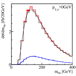
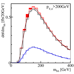
The obvious choice of side bands is, of course, the invariant mass of the two -jets reconstructing the Higgs. While for the signal we expect a peak around 125 GeV, possibly shifted towards lower values by final state radiation escaping the momentum reconstruction, background (including combinatorics) can be well described by a log-normal distribution. In Figure 3 we plot the invariant mass of the two un-associated -jets of events that have survived the initial selection cuts of Eqs.(3) and (4) and the top reconstruction algorithm. The relatively narrow mass peak of the signal is well separated from a broad feature of the backgrounds. Not all signal events can be associated with a parton–level Higgs momentum. In some cases the reason is missing final state radiation, in others it can be due to the -jet combinatorics.
The situation significantly improves once we introduce a cut on the reconstructed tops. Now the events under the Higgs peak are more and more dominated by the actual Higgs signal, and the signal peak separates cleanly from the broad maximum in the background shape. In Table 2 we show the rate of signal and background events with in the mass window of 90-130 GeV using the top reconstruction method to identify the Higgs decay products. This can be directly compared to the naive reconstruction methods from the previous section, summarized in Table 1. Requiring that one of the two reconstructed top quarks satisfy improves the signal–to–background ratio by a factor of two.
While at this stage the cut–and–count analysis is running out of steam, it might be useful to show that the bucket reconstruction of the two top decays gives us additional handles on the backgrounds. For example, we can require the reconstructed momenta of the reconstructed Higgs and tops to be central and not too widely separated in rapidity, as is typically the case for heavy particle production,
| (12) |
In Table 3 we show the corresponding signal and background rates. As can be seen, the ratio of signal to background is greatly improved. Taking the most aggressive criteria, requiring the leading reconstructed top to have GeV and the cut, we reach a , of which 70% of the signal -jets in the mass window are correctly identified from the Higgs decay. In general, this shows that the top reconstruction provides two handles that can improve the signal strength. First, it gives us a more accurate method to assign -jets to the Higgs decay, reducing the combinatorial background. Second, it gives us kinematic information for the event that can be exploited to discriminate signal events.
Clearly, the proposed bucket analysis is unlikely to be the last experimental word in extracting purely hadronic events from QCD background. However, our analysis shows that QCD and combinatorial backgrounds do not render this channel hopeless. Reconstructing the top decay products preferably in the slightly boosted regime can solve both problems and even leave the analysis with simple side bands, like the distribution.
IV Conclusion
We have demonstrated a method to extract the associated production of the Higgs along with top pairs in the fully hadronic channel, using the top buckets method or Ref. buckets to reconstruct the hadronic tops. Using this reconstruction technique nets us several useful advantages over more naive methods to reduce the very large backgrounds.
First, by having an accurate method of determining which two of the four -jets in the event should be assigned to the top pair, we can cut through the combinatorial problem of identifying the two -jets from the Higgs decay. Side bands with GeV or GeV can be used to determine the background shape and extract the background cross section after cuts. Second, the bucket algorithm not only identifies the -jets from the top decay, it also gives a good approximation of the top and Higgs momenta. This allows us to place additional cuts, for example on the transverse momenta of the top quarks or on the of the various parton–level objects. Both of them help to reject background. In particular, requiring a small boost of the top quarks eases the combinatorial problem tth_bb . Further, more detailed analyses may improve on the fairly crude cuts we have chosen in this proof–of–concept paper.
In this paper, we concentrated on demonstrating the stability of our reconstruction technique despite the potentially large simulation and theoretical uncertainties inherent to a QCD background consisting of four -jets with many extra un-tagged jets. Using both Alpgen and Sherpa, we have validated that the simulation issues are under control. However, our study also clearly shows that the theory uncertainties on this kind of backgrounds are hardly covered by a factor two on the rate prediction. These issues can be mitigated in the experiments by use of the ample side-bands that this analysis affords. In addition to the background dominated regions outside of the Higgs mass window, there are also many sidebands available, for example in the distribution of jet multiplicity.
Acknowledgments
MB and TP would like to thank the Aspen Center of Physics because the idea for this paper was born on a Snowmass ski lift. TP would furthermore like to thank the CCPP at New York University for their hospitality, which added Washington Square as a second location crucial to the progress of this paper. Fermilab is operated by Fermi Research Alliance, LLC, under contract DE-AC02-07CH11359 with the United States Department of Energy.
Appendix A Signal and background simulations
In this Appendix we will confirm that the analysis described in this paper does not critically depend on uncertainties in the way we compute our signal and backgrounds. For the signal and the background we primarily rely on Sherpa sherpa predictions with up to one additional hard jet merged using the Ckkw approach ckkw . For the signal we test our results using Madgraph madgraph , with up to one hard jet included in the Mlm scheme mlm . Both event samples are normalized to the next-to-leading order rate (extrapolated to 13 TeV) of 504 fb tth_nlo , times a Higgs branching ratio of 57.7%. This corresponds to 129 fb for the purely hadronic decay channel. In Table 4 we observe a small difference in the normalization of the two event samples. The reason is that as a cross check in the Madgraph simulation, we do not require hadronic top decays in the simulation. As a result, the decays to hadronic taus contribute to the signal. Our default Sherpa simulation conservatively does not include these events.
For the background we test the Sherpa simulation with up to one hard additional jet with an Alpgen alpgen simulation without additional hard jets. Again, both samples are normalized to the next-to-leading order rate of 1037 fb ttbb_nlo after the generator cuts GeV, , and . This rate is approximate because, in the absence of a next-to-leading order prediction for TeV, we are forced to first extract the factor for 14 TeV and the cuts of Ref. ttbb_nlo , including a regularizing cut on the invariant mass of the two bottom quarks. We then multiply our cross section at 13 TeV by this factor. This approach is not ideal, but better then just using the leading order prediction.
In Table 4 we see that the transverse momentum distributions for the “reconstructed” top quarks (which, for , do not correspond to any parton-level tops) from Alpgen are softer than for Sherpa. This effect comes from the generically harder jets of Ckkw merging, compared to those from the parton shower. In order to be conservative, we use the merged Sherpa results for our analysis. On the other hand, the difference of less than 20% is well within the theory uncertainties for this background.
As argued in Section II, the most dangerous background events should be correctly described by our Alpgen simulation of the background plus Pythia parton shower, as the required extra jets must be hard, and therefore well-modeled by the matrix-level process. With our merged Sherpa simulation of jet, we test several aspects of our main background simulation:
-
1.
We check if the events with two additional hard jets are indeed the leading background after the kind of global cuts proposed in Section II. This aspect is very important for the appropriate simulation of the QCD background in an actual analysis.
-
2.
We test if our analysis depends on the simulation of the second un-tagged jet either with the hard matrix element or through the parton shower. In this way we can estimate an important source of theory uncertainties.
-
3.
As a measure of the level of agreement between the two simulations we compute the merged Sherpa event rate with a consistent variation of the renormalization and factorization scales. Ideally, the two simulations should agree within this scale variation in the signal region of the buckets analysis. Because the merged Sherpa prediction includes some leading next-to-leading order contribution such a numerical agreement also indicates that our simulations should not be plagued by huge QCD corrections.
This extensive list of tests should give a clear answer to the question if purely hadronic searches can be done in the presence of the large QCD backgrounds. Finally, we point out that merged Sherpa simulations can define excellent side bands in the distribution jet_scaling , which together with side bands in should be sufficient to control the background rate in the signal region in an experimental analysis. Our results suggest that such an approach would require a merged simulation of with up to at least two hard light-flavor or gluon jets, which is beyond our CPU capabilities.
| Madgraph (merged) | Sherpa (merged) | Alpgen (shower) | Sherpa (merged) | |
| After acceptance Eqs.(3) and (4) | 1.390 | 1.197 | 7.903 | 8.363 |
| 2 tops tagged | 1.100 | 0.894 | 5.893 | 5.882 |
| GeV | 0.866 | 0.709 | 4.684 | 4.868 |
| GeV | 0.342 | 0.289 | 1.806 | 2.189 |
| GeV | 0.180 | 0.165 | 0.978 | 1.295 |
| GeV | 0.092 | 0.089 | 0.502 | 0.724 |
| Mass window GeV | ||||
| 2 tops tagged | 0.337 | 0.259 | 1.016 | 0.859 |
| GeV | 0.274 | 0.208 | 0.780 | 0.688 |
| GeV | 0.112 | 0.091 | 0.260 | 0.265 |
| GeV | 0.058 | 0.050 | 0.128 | 0.144 |
| GeV | 0.032 | 0.028 | 0.059 | 0.072 |
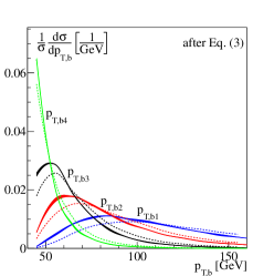
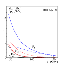
In Figure 4 we first show the normalized transverse momenta of the four -jets. The curves are set to unit normalization, as the significantly different cross section of the and the merged jets is almost entirely due to the different number of un-tagged jets in the events. In the left panel we see that the leading -jet agrees in the two approaches, while the second to fourth -jets become increasingly harder in the Alpgen sample. This is because, with two additional hard jets, the available recoil momentum is slightly larger. The sensitivity to the proper simulation of the recoil is also the reason why the Alpgen curves are not covered by the scale variation of the Sherpa simulation.
The results for the leading un-tagged jets in the right panel of Figure 4 look much less promising. The very different integrated rates under the curves reflect the additional events with only in the hard process plus any number of parton shower jets. This is particularly obvious for the first un-tagged jet, where the Sherpa simulation includes a majority of events with only one additional jet while the Alpgen sample will always include a second hard jet together with the first. For the second un-tagged jet the integrated rates in the distributions are similar for the two samples. The Alpgen simulation gives a significantly harder second jet from the matrix element while the second jet in our Sherpa sample (corresponding to the first jet from the parton shower) tends to be soft. The third un-tagged jet is the second parton shower jet in our Sherpa sample, while in the Alpgen simulation it is the first parton shower jet radiated from a harder core process. Both effects combined result in a significantly harder spectrum for the Alpgen sample. These distribution suggest that if our signal region should indeed require two or even three hard un-tagged jets to mimic top decay jets, the sample from Alpgen should be the appropriate, conservative estimate.
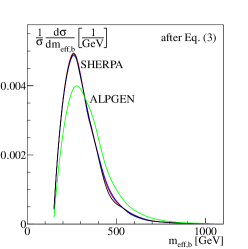
In the upper panels of Figure 5 we show the two relevant effective mass variables defined in Eq.(5). We require four -jets according to Eq.(3) and any number of un-tagged jets after Eq.(4). Unlike Figure 1 we now only show the different results for the background. In the upper left panel we again show the normalized observable from the multi- sector. The conclusion follows from the discussion of the transverse momenta of the four -jets: the dependence of the distribution on the simulation is small, clearly when we look at the Sherpa scale variation, but also in terms of the difference between Alpgen and Sherpa. The only difference is that the simulation with Alpgen predicts slightly harder multi- sectors.
In the upper central panel of Figure 5 we see that in the background region the difference in rate between the two simulations is again dramatic, and certainly not covered by the scale variation of the jets simulation with Sherpa. On the other hand, this result is entirely expected, and the difference becomes increasingly smaller once our analysis of the signal region requires something like GeV. Increasing the cut to GeV brings them into agreement within scale uncertainties. In that regime the bulk of the jet events do not contribute, so the two simulations should roughly agree within the scale variation of the Sherpa simulation. The upper right panel confirms that in the Alpgen simulation with the hard process also gives a harder spectrum in .
In the lower panels of Figure 5 we not only require four -jets following Eq.(3), but also at least two un-tagged jets fulfilling Eq.(4). Two such additional jets are implicitly required for any event passing the bucket analysis described in Section III. First, we see in the left panel that simply asking for two un-tagged jets suppresses the central prediction from the merged jets simulation to roughly half the prediction. Both distributions peak around 500 GeV, and the Alpgen rate is covered by the scale variation of the Sherpa simulation. In the central lower panel we compare the distributions for our default signal and background simulations after requiring four -tagged and two un-tagged jets. Finally, in the lower right panel we show the same distribution for all events passing the bucket analysis described in Section III. As compared to the acceptance cuts, Eqs.(3) and (4), there is hardly any change, which means that the improvements by the bucket analysis are more promising than the global cuts proposed in Section II, with the added advantage of avoiding shaping the background distributions, such as .
| Sherpa | Alpgen | +jets Sherpa | |||
| After acceptance Eqs.(3) and (4) | 1.197 | 54.420 | 18.825 | 25.812 | 50.974 |
| 2 tops tagged | 0.894 | 29.356 | 7.507 | 10.091 | 20.473 |
| GeV | 0.709 | 20.838 | 5.049 | 7.283 | 13.843 |
| GeV | 0.289 | 5.194 | 1.155 | 1.419 | 3.018 |
| GeV | 0.165 | 2.213 | 0.488 | 0.717 | 1.361 |
| GeV | 0.089 | 0.917 | 0.218 | 0.351 | 0.645 |
| Mass window GeV | |||||
| 2 tops tagged | 0.259 | 5.424 | 1.143 | 1.726 | 3.354 |
| GeV | 0.208 | 3.600 | 0.749 | 1.111 | 2.118 |
| GeV | 0.091 | 0.679 | 0.133 | 0.161 | 0.233 |
| GeV | 0.050 | 0.233 | 0.031 | 0.044 | 0.082 |
| GeV | 0.028 | 0.082 | 0.020 | 0.015 | 0.041 |
From the above comparison we expect that for an actual top and Higgs analysis the two background simulations should be fairly consistent once we probe sufficiently hard multi-jet configurations. The scale uncertainty of our Sherpa simulation determines the numerical level of this consistency. Moreover, in the signal phase space region the background simulation with parton shower should predict larger backgrounds and give us a conservative estimate. In Table 5 we show the different background rates after the buckets analysis. Indeed, the simulations agree roughly within the sizable scale uncertainties. The simulation with Alpgen gives the largest rate, in particular once we require large, signal-like values and sizable of the fake reconstructed top buckets. For the experimental analysis this implies firstly that the signal-to-background ratio for purely hadronic events at 13 TeV can be of the order 1/3. Second, the remaining number of signal events will be an issue for a cut-and-count analysis. Lastly, the uncertainties on the background simulation will require a careful background determination from side bands and control regions. Any kind of analysis which does not provide at least a slight mass peak in the distribution around 125 GeV would have a hard time convincing the authors of this study. Our buckets analysis will carefully ensure that this simple side band is clearly visible, in spite of the fact that this requirement might lead to a slightly reduced performance of our analysis.
Appendix B Top reconstruction
In this Appendix, we provide metrics concerning the reconstruction of the top pair, using the bucket method originally proposed in Ref. buckets , and described in detail in Section III. As every event contains exactly four -jets, reconstructing the tops leaves two -jets that can be identified as coming from the decay of the Higgs, thus we can reconstruct its momentum as well. While cuts on the top and Higgs kinematics are not critical to the analysis presented in this paper, for example a multivariate version of the same analysis would immediately be able to benefit from a valid bucket reconstruction.
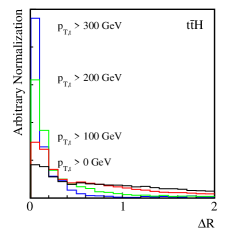
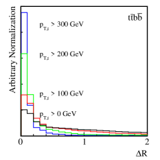
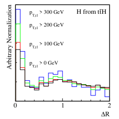
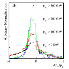
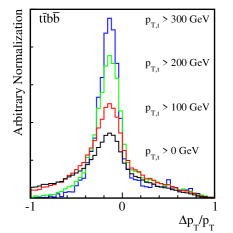
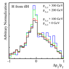
We can compare the magnitude and direction of the reconstructed top momenta to the true values of the parton–level tops, using Monte Carlo truth. As in Ref. buckets , the two kinematic variables we concentrate on are , defined between the parton–level top or Higgs and the closest of the two reconstructed tops or the reconstructed Higgs in the event, and , again taking the difference in between the parton–level object and the nearest bucket-reconstructed top or the reconstructed Higgs, normalized by the reconstructed . Figure 6 shows these distributions for both the signal and the irreducible background with real top quarks. Different lines correspond to the different reconstructed top cut for each bucket. For the Higgs plots (right column), these lines correspond to the different cuts on the leading reconstructed top in an event.
Defining a “good” reconstruction as and for the tops, we give in Table 6 the percentage of reconstructed tops in the signal and the background that are well-reconstructed. We also show the percentage of well-reconstructed Higgses in the signal sample. As can be seen, placing cuts on the reconstructed tops increases the purity of well-reconstructed tops and Higgses, though clearly this sacrifices total cross section.
| 0 GeV | 100 GeV | 150 GeV | 200 GeV | 250 GeV | 300 GeV | ||
|---|---|---|---|---|---|---|---|
| from | 0.357 | 0.515 | 0.643 | 0.759 | 0.820 | 0.856 | |
| 0.256 | 0.378 | 0.452 | 0.518 | 0.558 | 0.586 | ||
| and | 0.153 | 0.246 | 0.337 | 0.436 | 0.507 | 0.551 | |
| from | 0.415 | 0.563 | 0.681 | 0.777 | 0.837 | 0.860 | |
| 0.290 | 0.404 | 0.480 | 0.537 | 0.566 | 0.582 | ||
| and | 0.191 | 0.285 | 0.376 | 0.463 | 0.519 | 0.548 | |
| from | 0.206 | 0.223 | 0.246 | 0.278 | 0.290 | 0.312 | |
| 0.290 | 0.301 | 0.319 | 0.330 | 0.331 | 0.325 | ||
| and | 0.116 | 0.128 | 0.143 | 0.162 | 0.172 | 0.189 |
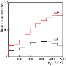
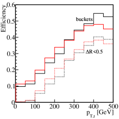
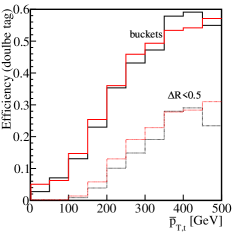
Finally, in Figure 7, we show the efficiencies for this algorithm as a function of the parton–level top , for several ranges of reconstructed . The left panel displays the acceptances for the selection Eqs.(3) and (4) as a function of . Note that the acceptance for sample is computed against the sample with the generation cut of GeV and . The central panel shows the efficiency for a single reconstructed top as a function of the parton–level top relative to the number in the left panel. The efficiencies for (black) and (red) are shown. The contributions for the buckets with a parton–level top found in are indicated by dotted lines. We see both channels have similar efficiencies after the acceptance cut. The right panel gives the double tag efficiency as a function of the average of the parton–level transverse momenta of the two tops. Note that our algorithm always tags two tops and the resulting efficiencies are similar to the central panel in number.
References
- (1) P. W. Higgs, Phys. Lett. 12, 132 (1964); P. W. Higgs, Phys. Rev. Lett. 13, 508 (1964); F. Englert and R. Brout, Phys. Rev. Lett. 13, 321 (1964).
- (2) G. Aad et al. [ATLAS Collaboration], Phys. Lett. B 716, 1 (2012); S. Chatrchyan et al. [CMS Collaboration], Phys. Lett. B 716, 30 (2012),
- (3) For an example analyses see M. Klute, R. Lafaye, T. Plehn, M. Rauch and D. Zerwas, Phys. Rev. Lett. 109, 101801 (2012); D. Lopez-Val, T. Plehn and M. Rauch, arXiv:1308.1979 [hep-ph].
- (4) D. E. Morrissey, T. Plehn and T. M. P. Tait, Phys. Rept. 515, 1 (2012).
- (5) for a pedagogical introduction see T. Plehn, Lect. Notes Phys. 844, 1 (2012) [arXiv:0910.4182].
- (6) For an update based on jet substructure analyses see T. Plehn, G. P. Salam and M. Spannowsky, Phys. Rev. Lett. 104, 111801 (2010).
- (7) A. Belyaev and L. Reina, JHEP 0208, 041 (2002); E. Gross and L. Zivkovic, Eur. Phys. J. 59, 731 (2009); C. Boddy, S. Farrington and C. Hays, Phys. Rev. D 86, 073009 (2012); P. Agrawal, S. Bandyopadhyay and S. P. Das, arXiv:1308.6511 [hep-ph].
- (8) F. Maltoni, D. L. Rainwater and S. Willenbrock, Phys. Rev. D 66, 034022 (2002); D. Curtin, J. Galloway and J. G. Wacker, arXiv:1306.5695 [hep-ph]; P. Agrawal, S. Bandyopadhyay and S. P. Das, arXiv:1308.3043 [hep-ph].
- (9) G. Aad et al. [ATLAS Collaboration], ATLAS-CONF-2012-102; G. Aad et al. [ATLAS Collaboration], JHEP 1301, 116 (2013); S. Chatrchyan et al. [CMS Collaboration], arXiv:1307.4617 [hep-ex]. Gregor Kasieczka, PhD thesis, Heidelberg University.
- (10) M. R. Buckley, T. Plehn and M. Takeuchi, JHEP 1308, 086 (2013).
- (11) S. Schumann, A. Renaud and D. Zerwas, JHEP 1109, 074 (2011).
- (12) M. H. Seymour, Z. Phys. C 62, 127 (1994).
- (13) T. Plehn and M. Spannowsky, J. Phys. G 39, 083001 (2012); A. Abdesselam et al., Eur. Phys. J. C 71, 1661 (2011); A. Altheimer et al., J. Phys. G 39, 063001 (2012).
- (14) A. Djouadi, J. Kalinowski and M. Spira, Comput. Phys. Commun. 108, 56 (1998).
- (15) S. Heinemeyer et al. [LHC Higgs Cross Section Working Group Collaboration], arXiv:1307.1347 [hep-ph].
- (16) M. L. Mangano, M. Moretti, F. Piccinini, R. Pittau and A. D. Polosa, JHEP 0307, 001 (2003).
- (17) J. Alwall, M. Herquet, F. Maltoni, O. Mattelaer and T. Stelzer, JHEP 1106, 128 (2011).
- (18) T. Sjostrand, S. Mrenna and P. Z. Skands, JHEP 0605, 026 (2006); T. Sjostrand, S. Mrenna and P. Z. Skands, Comput. Phys. Commun. 178, 852 (2008).
- (19) T. Gleisberg, S. .Hoeche, F. Krauss, M. Schönherr, S. Schumann, F. Siegert and J. Winter, JHEP 0902, 007 (2009).
- (20) S. Catani, F. Krauss, R. Kuhn and B. R. Webber, JHEP 0111, 063 (2001).
- (21) M. L. Mangano, M. Moretti, F. Piccinini and M. Treccani, JHEP 0701 (2007) 013.
- (22) W. Beenakker, S. Dittmaier, M. Kramer, B. Plumper, M. Spira and P. M. Zerwas, Nucl. Phys. B 653, 151 (2003); S. Dawson, C. Jackson, L. H. Orr, L. Reina and D. Wackeroth, Phys. Rev. D 68, 034022 (2003).
- (23) A. Bredenstein, A. Denner, S. Dittmaier and S. Pozzorini, Phys. Rev. Lett. 103, 012002 (2009); A. Bredenstein, A. Denner, S. Dittmaier and S. Pozzorini, JHEP 1003, 021 (2010); G. Bevilacqua, M. Czakon, C. G. Papadopoulos, R. Pittau and M. Worek, JHEP 0909, 109 (2009).
- (24) C. Englert, T. Plehn, P. Schichtel and S. Schumann, Phys. Rev. D 83, 095009 (2011); E. Gerwick, T. Plehn, S. Schumann and P. Schichtel, JHEP 1210, 162 (2012); S. El Hedri, A. Hook, M. Jankowiak and J. G. Wacker, JHEP 1308, 136 (2013).
- (25) J. Cammin, Thesis, BONN-IR-2004-06.
- (26) Y. L. Dokshitzer, G. D. Leder, S. Moretti and B. R. Webber, JHEP 9708, 001 (1997); M. Wobisch and T. Wengler, In “Hamburg 1998/1999, Monte Carlo generators for HERA physics” 270-279. [hep-ph/9907280].
- (27) T. Plehn, M. Spannowsky, M. Takeuchi, and D. Zerwas, JHEP 1010, 078 (2010);