Phonon induced Superconductivity of High Temperatures in Electrical Graphene Superlattices

Abstract

We discuss the BCS theory for electrons in graphene with a superimposed electrical unidirectional superlattice potential (SL). New Dirac points emerge together with van Hove singularities (VHS) linking them. We obtain a superconducting transition temperature $T_{c}$ for chemical potentials close to the VHS assuming that acoustic phonon coupling should be the dominant mechanism. Pairing of two onsite electrons with one electron close to the ${\bf K}$ and the other close to the $-{\bf K}$ point is the most stable pair formation. The resulting order parameter is almost constant over the entire SL.

I Introduction

The emergence of new interesting physics by the application of electrical and magnetical fields on graphene is one of the properties of this material. It was shown for example recently that new Dirac points can be opened in the energy spectrum by imposing an electrical SL on the graphene layer Talyanskii1 ; Brey1 ; Park2 . Most important in neutral graphene is that these new Dirac points are opened up in the lowest energy band. Other Dirac points emerge as linking points of two minibands Park1 ; Park5 at higher energies. New Dirac points were in fact found experimentally for graphene with Moiré SLs on underlying substrates Pletikosic1 ; Yankowitz1 and in unidirectional corrugated graphene monolayers Yan1 . Such points lead to unusual conductivity properties in SL systems Brey1 ; Park2 ; Dietel2 ; Dietel3 ; Burset1 ; Barbier2 ; Sun1 . Together with the new Dirac points also VHSs emerge in the density of states shown up as saddle points in the energy spectrum. The new Dirac points are linked by the saddle points.

Since the discovery of graphene there were attempts to find superconductivity in these materials. This is mainly motivated by the fact that superconductivity shows up experimentally in other carbon based materials with rather high critical temperatures $T_{c}$ for conventional superconductors as for example graphite intercalated ($T_{c}\lesssim 12K$) Weller1 ; Calandra1 and fullerite compounds ($T_{c}\lesssim 33K$) Gunnarson1 . Both forms of carbon based superconductors are mainly well described by the conventional phonon mediated BCS theory. The higher temperatures in the fullerite superconductors can be attributed to the high frequency of the innermolecular phonon modes being responsible for pairing in fullerites Varma1 . These phonon modes have around one order of magnitude higher frequencies than phonons mediating BCS superconductivity in metals Eisenstein1 . Similar high phonon frequencies are also found in the graphene phonon spectrum. Furthermore, theoretically it was shown that also graphane Savini1 , multilayer Kopnin1 and strained graphene Uchoa2 could lead to BCS instabilities with high temperatures. In Refs. Uchoa1, ; Kopnin2, it was shown theoretically that for pristine graphene at half filling a critical interaction value exists above which BCS pairing is possible. This is mainly due to a vanishing density of states at half filling. In both papers restrictions on the electronic pairing are made where either a coupling with total zero momentum Uchoa1 is considered or, more restrictively with an onsite s-wave pairing of one electron close to the ${\bf K}$ with another electron close to the ${\bf-K}$ valley Kopnin2 ; Uchoa2 . For small but non-zero chemical potentials gained by electrostatic doping, $T_{c}$ is still small. Except of the small density of states at these fillings one has to take also into account here the smallness of the optical electron-phonon coupling constant which is relevant in this regime Einenkel1 . The corresponding deformation potential for the coupling of electrons with longitudinal acoustic ${\bf\Gamma}$ phonons is much higher than of the other acoustic and optical phonon modes Suzuura1 ; Ishikawa1 ; Pisanec1 ; Dietel4 . This coupling mechanism should become relevant for larger chemical potentials when the corresponding Bloch Grüneisen temperature $\Theta_{\rm BG}=2\hbar k_{F}v_{s}$ in which $k_{F}$ is the Fermi-momentum and $v_{L}$ the phonon velocity, is in the regime of the Debye temperature Efetov1 . Here we use the fact that $T_{c}$ scales exponentially with the inverse square of the electron-phonon coupling, but only factorially with the energy cut-off $\sim\Theta_{\rm BG}/2$ for acoustic phonon coupling, or the main optical phonon frequency for optical phonon pairing. Note that in graphene the Debye frequency of the longitudinal acoustic ${\bf\Gamma}$ phonons is of similar magnitude as of the main optical phonons. With the application of a SL, the electron bands are effectively folded bringing the effective Grüneisen temperature also for low electrostatic doping potentials in the regime where the deformation potential coupling becomes relevant. This is one motivation to consider superconductivity in graphene superimposed by an SL. An additional motivation is the existence of low-lying VHSs in SL graphene which promises superconductivity with high $T_{c}$-values for chemical potentials close to the VHSs.

There are other possible sources of superconductivity than only phonon mediated superconductivity. One finds in the literature for example the Coulomb interaction as a possible source of pairing via the Kohn-Luttinger mechanism in graphene Gonzales1 ; Nandkishore1 ; Kiesel1 . This effect becomes most pronounced for energy bands when a VHS is existent. In pristine graphene one finds three in-equivalent saddle points producing a VHS at large energies linking the ${\bf K}$ and $-{\bf K}$ Dirac points. Such high chemical potentials can yet only be reached by chemical doping McChesney1 . It was shown in Ref. Gonzales1, that a possible $d+id$ wave instability with high $T_{c}$ can only be guaranteed when the saddle points producing the VHS are linked approximatively by nesting vectors. Such nesting vectors are not found for the VHSs in SL systems. Note that phonon-coupled BCS theory is not yet discussed for high chemical doped graphene in the literature. One reason is that phonon modes are sensitive on the special chemical doping which makes it rather complicated to carry out such calculations Calandra1 .

In the following, we will discuss the simplest case of BCS-type superconductivity in SL superimposed graphene mediated by acoustic phonons. We concentrate us hereby to the most interesting region of chemical potentials close to VHSs since this promises the highest $T_{c}$-values. Since we shall use analytically the role of the different possible superconducting order parameters in the SL system, our investigation can in principle be used when other superconducting coupling mechanisms become relevant.

The paper is structured as follows. In Sect. II we give first an introduction to the Bogoliubov-de Gennes (BdG) equation for superconductivity in graphene superimposed with an SL and discuss the transfer matrix formalism for solving this equation. Sect. III discusses the one-particle spectrum, and Sect. IV the phase diagram as a function of temperature.

II Electrical Superlattice

In the following we neglect corrections to BCS superconductivity expressions due to the repelling Coulomb interaction. Here we take into account that the unscreened interaction potential of electrons due to Coulomb interaction is of similar value as the attractive interaction potential from the Fröhlich Hamiltonian (c.f. Eq. (3)) for momentum transfer $k_{\rm DB}\approx 2.2/a$ calculated by using longitudinal acoustic electron-phonon coupling, where $k_{\rm DB}$ is the Debye momentum and $a\approx 1.4$Å  the interlattice distance. Due to the large momentum transfer, we can neglected in our calculation screening effects due to a possible substrate and further the inner graphene screening. For electron band widths much larger than the energy cut-off due to the electron-phonon interaction, retardation effects becomes important and an electron scatters with the phonon trace of another electron being not close in space at the same time Gunnarson1 ; Alexandrov1 . This leads to a suppression of the effective Couloumb interaction potential known as the so called Coulomb pseudopotential. This potential is strongly suppressed for superconductors where the density of states is large at the Fermi-surface Morel1 ; Sigrist1 . This is the case in the regime we are interested in when the chemical potential of the SL system lies close to a VHS. For small momentum transfer we can neglect the Coulomb interaction due to the large screening in the vicinity of the VHSs.

We discuss here the most simple representation of a SL being a symmetric two-step Kronig-Penney potential with a superlattice potential $V(x)=V\chi(x)$ where $\chi(x)={\rm sg}[\sin(2\pi x/d)]$. The function ${\rm sg}[x]$ is the sign of $x$, and $d$ is the wavelength of the SL. In the continuum approximation, the graphene Hamiltonian under consideration near the $\pm{\bf K}$ Dirac point is given for $d\gg a$ by Castro1

$$H_{\pm}=\hbar v_{F}(\pm\sigma_{1}\partial_{x}/i+\sigma_{2}\partial_{y}/i)+V(x)\,.$$ (1)

Here $\sigma_{1,2}$ are the Pauli matrices, while $v_{F}$ is the velocity of the electrons in graphene. In the following, we assume as in conventional superconductors spin singlet pairing, being most reasonable for phonon pairing. The formalism is then simplified considerably by taking into account the eigenvalue problem in the Nambu space with the eight component field ${\bf\Psi}(x)=(\phi^{K}_{A,\uparrow}\!,\!\phi^{K}_{B,\uparrow}\!,\!-i\phi^{-K}_{B,\uparrow}\!,\!i\phi^{-K}_{A,\uparrow}\!,\!(\phi^{-K}_{A,\downarrow})^{*}\!,\!(\phi^{-K}_{B,\downarrow})^{*}\!,\!i(\phi^{K}_{B,\downarrow})^{*}\!,\!-i(\phi^{K}_{A,\downarrow})^{*})$. The BdG-Hamiltonian is given by

$${\bf H}_{\rm BdG}=\left(\begin{array}[]{c c}\sigma_{0}\otimes(H_{+}-\mu)&\Delta\\ \Delta^{+}&-\sigma_{0}\otimes(H_{+}-\mu)\end{array}\right)$$ (2)

where $\sigma_{0}$ is the two-dimensional unit matrix. The condensate matrix $\Delta_{ij}$ is given by $\Delta_{ij}({\bf r})=(g/S^{2})\sum_{{\bf k},{\bf q}}\langle\Psi_{i}({\bf k}+{\bf q})\Psi^{+}_{4+j}({\bf k})\rangle\theta({\bf k}+{\bf q})\theta({\bf k})e^{i{\bf q}{\bf r}}$ where $S$ is the area of the system. The function $\theta({\bf k})$ is an energy cut-off given by $\theta({\bf k})\equiv\Theta[\omega_{\rm DB}^{*}-|\epsilon^{0}({\bf k}|)]$ for some canonical momentum ${\bf k}$ where $\Theta$ is the Heaviside function. Here $\epsilon^{0}({\bf k})$ is the energy of the lowest band of (2) for $\Delta=0$ (c.f. Eq. (12) below). We point out that ${\bf k}$ and ${\bf k}+{\bf q}$ are canonical momenta and not the Bloch momenta of the eigenfunctions. A sufficient condition that the BdG equation (2) is then a mean-field BCS decoupling equation for the exact superconducting problem by using the Fröhlich interaction approximation requires that the eigenfunctions of (2) for $\Delta_{ij}=0$ are localized on a circle in canonical momentum space for electrons with energies close to the chemical potential. That (2) together with $\Delta_{ij}$ in the canonical momentum basis is well defined requires further that the energy band $\epsilon^{0}({\bf k})$ is a unique function of the canonical momenta. Both assumptions will be shown below where we also determine the energy cut-off $\omega_{\rm DB}^{*}$.

Let $g$ denote the phonon induced coupling constant of the Fröhlich Hamiltonian for graphene. Due to the inhomogeneity of the SL in space it is not appropriate to consider a constant pairing function. Instead we shall assume an order parameter which is step-like of the form $\Delta_{ij}({\bf r})=\Delta^{c}_{ij}+\Delta^{s}_{ij}\chi(x)$, where $\Delta^{c}_{ij}$ and $\Delta^{s}_{ij}$ are constant.

The acoustic electron-phonon energy due to deformation potential coupling is given by $H_{\rm ep}=g_{\rm ep}\int d{\bf r}(u_{xx}+u_{yy})|{\bf\Psi}({\bf r})|^{2}$ where $g_{\rm ep}$ is the deformation potential and $u_{ij}$ is the strain tensor of the graphene lattice. The effective Fröhlich interaction coupling constant $g$ is then given by $g=g_{\rm ep}^{2}2/v_{L}^{2}\rho_{C}$ where $v_{L}\approx 21.1\cdot 10^{3}m/s$ is the longitudinal acoustic phonon velocity, and $\rho_{C}\approx 761\cdot 10^{-9}kg/m^{2}$ the density of carbon atoms. This leads to $g\approx 6\cdot 10^{-19}m^{2}\rm eV$. Here we work with a deformation potential of $g_{\rm ep}\approx 25\rm{\rm eV}$. The corresponding Fröhlich coupling constant for out-of-plane acoustic phonons is by a factor $\omega_{\rm DB}^{2}/\kappa_{0}^{2}\ll 1$ smaller, where $\kappa_{0}$ is the bending constant Dietel1 and $\omega_{\rm DB}$ is the Debye frequency for longitudinal acoustic phonons. The Fröhlich interaction Hamiltonian is then

$$H_{\rm Fr}\!=\!-\frac{g}{S^{3}}\!\!\sum_{i,j\leq 4}\sum_{{\bf k},{\bf k}^{\prime},{\bf q}}\!\!\!\!\Psi_{4+j}(\!{\bf k}\!)\Psi^{+}_{i}(\!{\bf k}+{\bf q}\!)\Psi_{i}(\!{\bf k}^{\prime}+{\bf q}\!)\Psi^{+}_{4+j}(\!{\bf k}^{\prime}\!)$$

$$\qquad\qquad\times\theta({\bf k})\theta({\bf k}+{\bf q})\theta({\bf k}^{\prime}+{\bf q})\theta({\bf k}^{\prime})\,.$$ (3)

We obtain from (1) and (3) by using a mean-field decoupling the BdG Hamiltonian (2) where the BdG-matrix has then in general ten unknown complex parameters $\Delta_{ij}$. Here we assume that $\Delta_{ij}=(-1)^{i+j+1}\Delta_{4-i,4-j}$ for $i,j\in\{1,2\}$, and $\Delta_{31}=-\Delta_{42}$, $\Delta_{13}=-\Delta_{24}$ when we take into account spin singlet pairing in the original graphene fields. One can simplify this matrix further under the assumption that the condensate does not break the time-inversion symmetry as well as the mirror symmetry with respect to the $x$ and $y$-axis, where we choose that the mirror operation with respect to the $x$-axis should lead to an interchanging of $A$, $B$ atoms if $A$ and $B$ denotes the inequivalent carbon atoms in the fundamental cell. These assumptions will be justified further below. The time inversion transformation on a graphene spinor is given by ${\cal T}\phi^{K}_{A,\uparrow}=(\phi^{-K}_{A,\downarrow})^{*}$, defined modulo the interchange $A\leftrightarrow B$, $\uparrow\leftrightarrow\downarrow$ and $K\leftrightarrow-K$. Similar is also assumed for the $x$-axis mirror transformation ${\cal S}_{x}\phi^{K}_{A,\uparrow}(y)=\sigma_{1}\phi^{K}_{B,\uparrow}(-y)$ and the $y$-axis mirror transformation ${\cal S}_{y}\phi^{K}_{A,\uparrow}(x)=\phi^{-K}_{A,\uparrow}(d/2-x)$. By taking into account the invariance of the condensate under these operations, we obtain $\Delta=\Delta_{1}+\Delta_{2}+\Delta_{3}+\Delta_{4}$ with

$$\Delta_{1}=d_{1}\sigma_{3}\otimes\sigma_{0}\,,\,\Delta_{2}=d_{2}\sigma_{0}\otimes\sigma_{1}\,,\,$$

$$\Delta_{3}=d_{3}\sigma_{2}\otimes\sigma_{2}\,,\,\Delta_{4}=d_{4}\sigma_{1}\otimes\sigma_{3}\,,$$ (4)

where $d_{i}\in\mathbb{R}$. We now separate $d_{i}$ according to $d_{i}=d_{i}^{c}+d_{i}^{s}\chi(x)$ where $d_{i}^{c}$, $d_{i}^{s}$ are constants. In the following, we solve the eigenvalue equation ${\bf H}_{\rm BdG}{\bf u}({\bf r}^{\prime})=\epsilon\,{\bf u}({\bf r}^{\prime})$ by using the transfer matrix method Arovas1 ; Dietel2 . With the help of ${\bf u}(x,y)\!=\!e^{ik_{y}y}{\bf u}(x)$, the eigenfunctions of the lowest band are given by ${\bf u}(x)={\bf\Lambda}(x){\bf u}(0)$. With this definition we obtain from the Schrödinger equation with the Hamiltonian (2) the following equation for the transfer matrix ${\bf\Lambda}$

$$\frac{1}{i}\partial_{x}{\bf\Lambda}(x)\!=\!-\!\sigma_{3}\!\otimes\!\sigma_{0}\!\otimes\!\sigma_{3}\big{(}k_{y}\sigma_{3}\!\otimes\!\sigma_{0}\!\otimes\!\sigma_{2}\!+\!V(x)\sigma_{3}\!\otimes\!\sigma_{0}\!\otimes\!\sigma_{0}$$

$$\qquad\qquad\;\;\,-\epsilon\sigma_{0}\otimes\sigma_{0}\otimes\sigma_{0}+\sigma_{1}\otimes\Delta\big{)}{\bf\Lambda}(x)\,.$$ (5)

This equation is solved perturbatively with respect to the small condensate matrix $\Delta$, where the corresponding terms are denoted by ${\bf\Lambda}={\bf\Lambda}^{0}+{\bf\Lambda}^{1}+{\bf\Lambda}^{2}+\ldots$. We obtain from (5) that for $\Delta=0$, ${\bf\Lambda}={\bf\Lambda}^{0}$ is diagonal within the valley and electron-hole sectors. We denote the valley electron-hole submatrizes by $\Lambda^{0}_{\pm}=\sum_{i}\sigma_{i}{\rm Tr}[(\sigma_{0}\pm\sigma_{3})\otimes\sigma_{0}\otimes(\sigma_{i})^{*}\cdot{\bf\Lambda}^{0}]/4$. This leads to

$$\Lambda_{\pm}^{0}(x)\!=\!\lambda_{0}(x)\Theta\!\left(\!\frac{d}{2}-x\!\right)\!+\!\lambda_{d/2}(x)\lambda_{0}\!\left(\!\frac{d}{2}\!\right)\!\Theta\!\left(\!x-\frac{d}{2}\!\right)\,,$$ (6)

where

$$\lambda_{x_{0}}(x)\!=\!\cos\!\left[\!\frac{\alpha_{E_{\pm}}(x)2(x-x_{0})}{d}\!\right]\!\!\sigma_{0}\!+\!\frac{\sin\!\left[\!\frac{\alpha_{E_{\pm}}(x)2(x-x_{0})}{d}\!\right]\!}{\alpha_{E_{\pm}}(x)}M_{\pm}$$ (7)

with

$$M_{\pm}=k_{y}\sigma_{3}+[E_{\pm}-V(x)]\sigma_{2}/\hbar v_{F}\,.$$ (8)

Here $E_{\pm}=\pm\epsilon+\mu$ and

$$\alpha_{E_{\pm}}(x)=\{[(E_{\pm}-V(x))/\hbar v_{F}]^{2}-k_{y}^{2}\}^{1/2}d/2\,.$$ (9)

We can now calculate the energy spectrum for $\Delta=0$ by using the Bloch condition

$$\Lambda_{\pm}^{0}(d)u_{\pm}^{0}(0)=e^{ik_{x}d}u_{\pm}^{0}(0)$$ (10)

which is effectively an eigenvalue equation for $\Lambda^{0}_{\pm}(d)$ where the Bloch condition demands that the eigenvalue is a phase. By using the mirror symmetry of the SL with respect to the axis $x=d/4$, we obtain that eigenvalues of the transfermatrix $\Lambda^{0}_{\pm}(d)$ to the Hamiltonian must come in pairs $e^{ik_{x}d}$ and $e^{-ik_{x}d}$, where $k_{x}$ and $-k_{x}$ are complex numbers in general. In the case of the Bloch eigenvalue equation (10) this leads to ${\rm Tr}[\Lambda_{\pm}^{0}(d)]=2\cos(k_{x}d)$, where

$${\rm Tr}[\Lambda_{\pm}^{0}(d)]=2\cos[\alpha_{E_{\pm}}(d/4)]\cos[\alpha_{E_{\pm}}(3d/4)]$$

$$-2\frac{\sin[\alpha_{E_{\pm}}(d/4)]\cos[\alpha_{E_{\pm}}(3d/4)]}{\alpha_{E_{\pm}}(d/4)\alpha_{E_{\pm}}(3d/4)}[\tilde{k}_{y}^{2}-(\tilde{E}_{\pm}^{2}-\tilde{V}^{2})].$$ (11)

For the energy dispersion in the lowest band, we obtain for large SL potentials $\alpha_{0}\gg 1$ and $|\tilde{E}\tilde{V}|\ll\alpha_{0}$ from (11) the eigenvalues Barbier1 ; Dietel3

$$\tilde{\epsilon}_{\pm}^{0}=\!\!\pm(s\hat{\alpha}^{2}_{0}\sqrt{\tilde{k}^{2}_{x}+|\hat{\Gamma}|^{2}\tilde{k}_{y}^{2}}-\tilde{\mu})\,.\\$$ (12)

Here $\hat{\Gamma}=\sin[\alpha_{0}]e^{i\alpha_{0}}/\alpha_{0}$, $\hat{\alpha}_{0}=\alpha_{0}/\tilde{V}$. We define dimensionless quantities $\tilde{x}\equiv xd/2\hbar v_{F}$ for quantities $x$ having the dimension of energy and $\tilde{k}\equiv kd/2$ when $k$ has as an inverse length dimension. The Bloch momentum in $x$-direction is restricted to $-\pi/2\leq\tilde{k}_{x}\leq\pi/2$. The parameter $s=1$ denotes the conduction band and $s=-1$ the valence band. We show in the left panel in Fig. 1 the approximation to the lowest lying energy band $\tilde{\epsilon}_{+}^{0}$ (12) (solid curves) and its exact counterpart (dotted curves) at $k_{x}=0$ and $\mu=0$, $s=1$ for various SL potentials $\tilde{V}$. We obtain a good agreement between both curves except at the outer boundary of the folded region where $\tilde{k}_{y}/\tilde{V}\approx 1$. Here we find $|\tilde{E}\tilde{V}|/\alpha_{0}\sim 1$ close to the VHSs, implying a breakdown of the expansion. The solution $u^{0}_{\pm}(0)$ is given in the regime $|\tilde{E}\tilde{V}|\ll\alpha_{0},\alpha_{0}\gg 1$ by

$$u^{0}_{\pm}(0)\approx\left(\begin{array}[]{c}\frac{\cos(\alpha_{0})\sin(\alpha_{0})}{\alpha_{0}}\tilde{k}_{y}+i\tilde{k}_{x}\\ i\frac{1}{\hat{\alpha}_{0}^{2}}\,\tilde{E}_{\pm}+i\frac{\sin^{2}(\alpha_{0})}{\alpha^{2}_{0}}\tilde{V}\tilde{k}_{y}\end{array}\right)\,.$$ (13)

We shall denote the vector components by $u^{0}_{\pm}(0)=(A+i\tilde{k}_{x},iB)^{T}$. From (12) we obtain an oscillatory behavior of the lowest energy band as a function of $k_{y}$. New Dirac points emerge at ${\bf k}=0$ for $\tilde{V}\in\mathbb{N}\pi$. We compare in Fig. 1 Eq. (12) with a numerical solution of (10). The new Dirac points are shifted along the y-axis in ${\bf k}$-space for increasing $\tilde{V}$. Now we focus on the higher energy saddle points building singularities in the density of states. The figure shows that even in this energy regime the approximation (12) is justified. Saddle points are quite interesting in forming a high-temperature BCS state when the chemical potential is close to the VHS. By using (12), we obtain for the density of states $\nu(\epsilon)$ per spin and valley close to a VHS at energies $E^{n}_{+}=\epsilon^{0}_{+}(0,k^{n}_{y})+\mu$, originating from a saddle point with momentum $k_{y}=k^{n}_{y}$ and $k_{x}=0$ for $\alpha_{0}\gg 1$

$$\nu(\epsilon)\approx\frac{\tilde{\nu}_{0}}{\hbar v_{F}d}\ln\left(\frac{16\tilde{W}^{2}_{\rm VHS}}{|(\tilde{\epsilon})^{2}-(\tilde{E}_{+}^{n})^{2}|}\right)\,,$$ (14)

$$\tilde{\nu}_{0}=\frac{\sqrt{2}}{\pi^{2}}\frac{|\tilde{E}_{+}^{n}|\tilde{V}^{4}}{(\tilde{k}^{n}_{y})^{2}\alpha^{2}_{0}}\frac{1}{\sqrt{\frac{1}{2}+\cos^{2}(\alpha_{0})}}\,,$$

where $\tilde{W}_{\rm VHS}={\rm min}[\hat{\alpha}^{2}_{0}\pi/2,2|\tilde{\mu}|]$ is the width of the VHS. We obtain from (12) the relation $\tan(\alpha_{0})\approx(\tilde{k}^{n}_{y})^{2}/\alpha_{0}$ for the momentum $\tilde{k}^{n}_{y}$ of the $n$-th saddle point in the energy spectrum where $n=1$ corresponds to the outermost saddle point. The solution of $\tan(\alpha_{0})\approx(\tilde{k}^{n}_{y})^{2}/\alpha_{0}$ can be approximated for the outer saddle points by $\tilde{k}^{n}_{y}\approx\pm\sqrt{\tilde{V}^{2}-(\pi/2+n\pi)^{2}}$ for $n\in\{1,\ldots,[\tilde{V}/\pi]-1\}$. Here $[x]$ is the largest integer value smaller than $x$. The saddle point closest to the central Dirac point has then still to be determined numerically by $\tan(\alpha_{0})\approx(\tilde{k}^{n}_{y})^{2}/\alpha_{0}$.

Due to the oscillatory behavior of the energy band we obtain that even for small chemical potentials, electrons with energies close to the chemical potential can scatter with a large momentum transfer. This is relevant when determining the energy cut-off within BCS theory, which we denoted $\omega_{\rm DB}^{*}$. By using (6)–(10) with (13) we obtain that the lowest band wavefunctions are localized around the canonical momenta $k_{x}\approx\pm\alpha_{0}2/d$ and $k_{y}$. This then leads to the energy cut-off for acoustic ${\bf\Gamma}$-phonon scattering $\omega_{\rm DB}^{*}\approx{\rm min}[V/\hbar v_{F}k_{\rm DB},1]\omega_{\rm DB}$.

As it was mentioned in the introduction, the energy cut-off for graphene without an SL due to acoustic electron-phonon scattering is in general much smaller being, $\omega_{\rm DB}^{*}\approx(\mu/\hbar v_{F}k_{\rm DB})\omega_{\rm DB}$.

III One-particle spectrum

By using (5) we are now able to calculate the $\Delta$ dependent correction terms to ${\bf\Lambda}$. With the abbreviation $\hat{\bf\Delta}(x)=(-\sigma_{3}\otimes\sigma_{0}\otimes\sigma_{3})\cdot(\sigma_{1}\otimes\Delta)$ we obtain

$${\bf\Lambda}^{1}(x)=i{\bf\Lambda}^{0}(x)\int^{x}_{0}dx^{\prime}({\bf\Lambda}^{0})^{-1}(x^{\prime})\hat{{\bf\Delta}}(x^{\prime}){\bf\Lambda}^{0}(x^{\prime})\,,$$ (15)

$${\bf\Lambda}^{2}(x)=-{\bf\Lambda}^{0}(x)\int^{x}_{0}dx^{\prime}({\bf\Lambda}^{0})^{-1}(x^{\prime})\hat{{\bf\Delta}}(x^{\prime}){\bf\Lambda}^{0}(x^{\prime})$$ (16)

$$\qquad\qquad\times\int^{x^{\prime}}_{0}dx^{\prime\prime}({\bf\Lambda}^{0})^{-1}(x^{\prime\prime})\hat{{\bf\Delta}}(x^{\prime\prime}){\bf\Lambda}^{0}(x^{\prime\prime})\,.$$

Here we use ${\bf\Lambda}^{0}=\sum_{p\in\{+,-\}}(\sigma_{0}+p\sigma_{3})\otimes\sigma_{0}\otimes\Lambda^{0}_{p}/2$. In the following, we calculate perturbationally the eigenvalues of the transfermatrix ${\bf\Lambda}(d)$ where ${\bf\Lambda}^{1}$ and ${\bf\Lambda}^{2}$ are seen as perturbations to ${\bf\Lambda}^{0}$.

We point out that standard Rayleigh-Schrödinger perturbation theory is not applicable here since the transfer matrices ${\bf\Lambda}^{0}$ or ${\bf\Lambda}$, respectively, are neither unitary nor hermitian. This is due to the fact that the matrix on the right hand side in Eq. (5) is not hermitean. But this matrix is hermitian with respect to the quadratic form $\langle{\bf u}|{\bf v}\rangle_{Q}\equiv\langle\sigma_{3}\otimes\sigma_{0}\otimes\sigma_{3}{\bf u}|{\bf v}\rangle$. Thus it does lead to the unitarity of ${\bf\Lambda}$ and ${\bf\Lambda}^{0}$ with respect to this form. Note that this quadratic form is not positive definite. In the Bloch regime where the eigenvalues are a pure phase factor, different eigenvalues are orthogonal with respect to the $Q$-form. One can now show that standard Rayleigh-Schrödinger perturbation can be used after all by substituting the quadratic form $\langle{\bf u}|{\bf v}\rangle_{Q}$ for all expressions where normally the cartesian scalar product $\langle{\bf u}|{\bf v}\rangle$ is used. This includes also the normalization of the basis functions (13).

In order to calculate the matrix elements of the operators (15), (16) we have taken into account the degeneracy of the eigensystem of ${\bf\Lambda}^{0}$. In zero’s order perturbation we obtain degenerate eigenstates. With the abbreviation $e_{i}$ ($i=1,\ldots,4$) for the cartesian basis in four-dimensional space, we obtain for the eigenvectors of ${\bf\Lambda}^{0}$, $u_{+}^{0}\otimes e_{1}$, $u_{+}^{0}\otimes e_{2}$ with eigenvalues of either $e^{+ik^{+}_{x}d}$ and $e^{-ik^{+}_{x}d}$ in the particle sector and $u_{-}^{0}\otimes e_{3}$, $u_{-}^{0}\otimes e_{4}$ with eigenvalues $e^{+ik^{-}_{x}d}$ and $e^{-ik^{-}_{x}d}$ in the hole sector. Here $k_{x}^{\pm}$ is given by $\tilde{k}_{x}^{\pm}=\sqrt{\tilde{E}_{\pm}^{2}/\hat{\alpha}^{4}_{0}-|\hat{\Gamma}|^{2}\tilde{k}_{y}^{2}}$. Note that ${\bf\Lambda}^{1}$ and ${\bf\Lambda}^{2}$ can in first approximation only connect states which are in the lowest band, i.e. $\tilde{k}^{\pm}_{x}\leq\pi/2$. By denoting $M_{\pm V}=k_{y}\sigma_{3}\mp V\sigma_{2}/\hbar v_{F}$ we obtain for $\alpha_{0}\gg 1$

$${\bf\Lambda}^{1}(d)\approx i\frac{d}{4}\bigg{[}{\bf\Lambda}^{0}(d)\hat{\bf\Delta}_{V}\left(\frac{d}{4}\right)\!\!+\!\hat{\bf\Delta}_{-V}\left(\frac{3d}{4}\right){\bf\Lambda}^{0}(d)\bigg{]},$$ (17)

$${\bf\Lambda}^{2}(d)\approx-\frac{d^{2}}{16}\bigg{(}\frac{1}{2}\bigg{\{}{\bf\Lambda}^{0}(d)\left[\hat{\bf\Delta}_{V}\left(\frac{d}{4}\right)\right]^{2}\!\!\!+\!\left[\hat{\bf\Delta}_{-V}\left(\frac{3d}{4}\right)\right]^{2}$$

$$\quad\quad\quad\times{\bf\Lambda}^{0}(d)\bigg{\}}+\hat{\bf\Delta}_{-V}\!\left(\frac{3d}{4}\right)\!{\bf\Lambda}^{0}(d)\hat{\bf\Delta}_{V}\!\left(\frac{d}{4}\right)\bigg{)}$$ (18)

where $\hat{\bf\Delta}_{\pm V}=\hat{\bf\Delta}-M_{\pm V}\hat{\bf\Delta}M_{\pm V}$. Next we calculate the matrix elements of ${\bf\Lambda}^{1}(d)$, ${\bf\Lambda}^{2}(d)$ with respect to the basis $u^{0}_{\pm}\otimes e_{i}$. Here we can restrict ourselves to leading order in $\epsilon^{0}$ and $k_{x}^{\pm}$ justified for chemical potentials close to a VHS. We obtain $u^{0}\equiv u_{-}^{0}\approx u_{+}^{0}$ with $\Lambda_{ij}=\langle u^{0}\otimes e_{i}|{\bf\Lambda}^{1}(d)|u^{0}\otimes e_{j}\rangle_{Q}$ for $i=1,\ldots,4$

$${\Lambda}_{31}^{1}(d)={\Lambda}_{13}^{1}(d)={\Lambda}_{24}^{1}(d)={\Lambda}_{42}^{1}(d)$$

$$\quad\quad\approx-\frac{4\tilde{V}[d^{c}_{1}\tilde{V}(A^{2}+B^{2}+\tilde{k}^{+}_{x}\tilde{k}^{-}_{x})+2d^{s}_{1}\tilde{k}_{y}AB]}{\tilde{V}^{2}-\tilde{k}_{y}^{2}},$$

$${\Lambda}_{32}^{1}(d)=-{\Lambda}_{23}^{1}(d)={\Lambda}_{14}^{1}(d)=-{\Lambda}_{41}^{1}(d)\,,$$ (19)

$$\quad\quad\approx i\frac{4\tilde{k}_{y}[d^{s}_{3}\tilde{V}(A^{2}+B^{2}+\tilde{k}^{+}_{x}\tilde{k}^{-}_{x})+2d^{c}_{3}\tilde{k}_{y}AB]}{\tilde{V}^{2}-\tilde{k}_{y}^{2}}\,.$$

In contrast to (19), the matrix elements ${\Lambda}_{ij}^{2}(d)\not=0$ are much more complicated, being also a function on the condensates $d_{2}$ with prefactors similar to (19). We even include in (19) a subleading $\tilde{k}^{2}_{x}$-term, which becomes relevant for the $d_{1},d_{3}$ dependence of the spectrum when the $k_{y}$ momentum lies not close to the saddle point.

To zero’s order in $\Delta$, we find two different $\tilde{\epsilon}^{0}$-regimes within Rayleigh-Schrördinger perturbation theory. For small $|\tilde{\epsilon}^{0}|$ where $k_{x}^{+}\approx k_{x}^{-}$ we find approximately a fourfold degenerate ground state with momentum $k_{x}^{+}$ in the ${\bf K}$ and $-{\bf K}$ valleys in the electronic sector, and $k_{x}^{-}$ in the ${\bf K}$ and $-{\bf K}$ valleys in the hole sector. The same holds for the $-k_{x}^{\pm}$ momenta. This degeneracy is lifted by using ${\bf\Lambda}^{1}(d)$ within first order perturbation theory. The energy spectrum is then dominated by the first order energy with respect to ${\bf\Lambda}^{1}(d)$.

For larger $|\tilde{\epsilon}^{0}|$ where $k_{x}^{+}\not=k_{x}^{-}$, we find a two-fold degeneracy corresponding to the $k_{x}^{+}$-state in the ${\bf K}$, $-{\bf K}$ electron valleys and a further degenerate ground state with $k_{x}^{-}$ in the ${\bf K}$, $-{\bf K}$ hole valleys. The same holds for the $-k_{x}^{\pm}$ momenta. The electron and hole valleys are not degenerate with each other in this case. The degeneracy for small $|\tilde{\epsilon}^{0}|$ where $|\tilde{\mu}\tilde{\epsilon}^{0}|\ll 1$ is lifted by first order perturbation theory with respect to ${\bf\Lambda}^{2}(d)$ in this case. On the other hand the first order energies with respect to ${\bf\Lambda}^{2}(d)$ can be neglected in comparison to the second order energies with respect to ${\bf\Lambda}^{1}(d)$.

To simplify our condensate search further, we will first consider only the $d_{1}$ dependence of the energy spectrum setting $d_{i}=0$ for $i\not=1$. By taking into account the consideration following (10) we obtain ${\rm Tr}[\Lambda_{\pm}(d)]+D_{\pm}=2\cos(k_{x}d)$ with

$$D_{\pm}\approx\pm{\rm min}\left[\frac{|T_{1}|}{4B},\frac{|T_{1}|^{2}}{64B^{2}|\tilde{\mu}\tilde{\epsilon}_{\pm}^{0}|\hat{\alpha}_{0}^{4}}\right]{\rm sgn}[\tilde{\mu}\tilde{\epsilon}^{0}_{\pm}]\Theta(\pi/2-\tilde{k}^{\mp}_{x})\,,$$ (20)

$$T_{1}=-\frac{4\tilde{V}}{\alpha_{0}^{2}}[\tilde{d}_{1}^{c}\tilde{V}(A^{2}+B^{2}+\tilde{k}^{2}_{x})+2\tilde{d}_{1}^{s}\tilde{k}_{y}AB]\,.$$ (21)

With the help of (12) we obtain for the branch of the energy spectrum being mainly influenced by BCS pairing for $|\tilde{\epsilon}^{0}|\ll|\tilde{\mu}|$

$$\tilde{\epsilon}_{\pm}\approx\pm\left(s\sqrt{(\tilde{\epsilon}_{\pm}^{0}\pm\tilde{\mu})^{2}+D_{\pm}/\hat{\alpha}^{4}_{0}}-\tilde{\mu}\right)$$

$$\quad\approx\pm{\rm sgn}[\tilde{\epsilon}^{0}_{+}]\sqrt{(\tilde{\epsilon}^{0}_{+})^{2}+D^{2}}\,,$$ (22)

with $D=D_{c}(d^{c}_{1},d^{s}_{1})$ where

$$D_{c}(d^{c}_{1},d^{s}_{1})=\frac{1}{\hat{\alpha}_{0}^{4}}\frac{|T_{1}|}{8B\tilde{\mu}}\Theta(\pi/2-\tilde{k}^{-}_{x})\,.$$ (23)

Note that in (22) with (12), the band parameter $s$ has to be chosen such that $|\tilde{\epsilon}^{0}_{+}|\ll|\tilde{\mu}|$, i.e. $s={\rm sgn}[\tilde{\mu}]$. The energy bands in (22) are doubly degenerated. This degeneracy is lifted when going beyond the lowest approximation used here.

The energy spectrum (22) with (23) has now a similar form as the energy spectrum of metals within the standard BCS theory. This point can be elaborated further by taking into account that (2) with (4) where only $d_{1}^{c}\not=0$ but $d_{1}^{s}=0$ and $d_{i}^{c},d_{i}^{s}=0$ for $i\not=1$, can be diagonalized by using standard Bogoljubov theory. This is based on the fact that $\Delta$ is comuting with $H_{+}$. This leads to the energy spectrum (22) with (23) where now $D_{c}=\tilde{d}_{1}^{c}$. This means that we should find $D_{c}(1,0)\approx 1$ in expression (23) in order to have a good approximation in hand.

We show in Fig. 1 $D_{c}(1,0)$ for various SL potentials $\tilde{V}$ and chemical potentials $\tilde{\mu}$ as a function of the rescaled momentum $\tilde{k}_{y}/\tilde{V}$ (left inset) and $\epsilon^{+}_{0}=0$. The curve segments which are absent in the figure are where $0\leq\tilde{k}_{x}^{+}\leq\pi/2$ is not fulfilled. Right panel in Fig. 1 shows $D_{c}(1,0)$ and $D_{c}(0,1)$ calculated at $\tilde{k}_{y}$-momenta and chemical potentials $\tilde{\mu}$ of the saddle point for the VHS singularities $n=1,\ldots,[\tilde{V}/\pi]$. We obtain from the figure or (13), respectively, that for large $\tilde{V}$ and small $n$ (outer VHSs), $D_{c}(1,0)$ is growing to infinity which can be avoided by taking into account higher order corrections in $\tilde{E}\tilde{V}/\tilde{\alpha}_{0}$ in (13) (c.f. caption of Fig. 1). From the right panel in Fig. 1, we obtain that the largest $D_{c}(0,1)$ value is reached for the outermost VHS with $n=1$ where $\tilde{V}\approx 4$ with value $D_{c}(0,1)\approx 0.3$. A further exceptional SL potential for $n=1$ is given by $\tilde{V}=6.66$ where $D_{c}(0,1)$ is vanishing. We show in the right inset in Fig. 1 the energy spectrum $\tilde{\epsilon}_{+}$ as a function of $d^{s}_{1}$ for $d^{c}_{1}=0$ using these both exceptional SL potentials and further the SL potential $\tilde{V}=4\pi$ ($n=1$) to gain a better insight what is happening with the spectrum in the outer VHSs for large $\tilde{V}$. We compare our results in the figure with a numerically determined energy spectrum for the same values using a numerically evaluated transfermatrix method similar to (5)–(10).

Summarizing we obtain from Fig. 1 that the agreement of our approximations with exact and numerical results are good for small $\tilde{V}\gtrsim 1$ but also for $\tilde{V}\gg 1$ for the inner valleys. The approximation becomes less good for the outermost valleys. The reason lies in the expansion parameters $1/\alpha_{0}$ and $\tilde{E}V/\alpha_{0}$ which we used in our approximation in order to derive (22), (23).

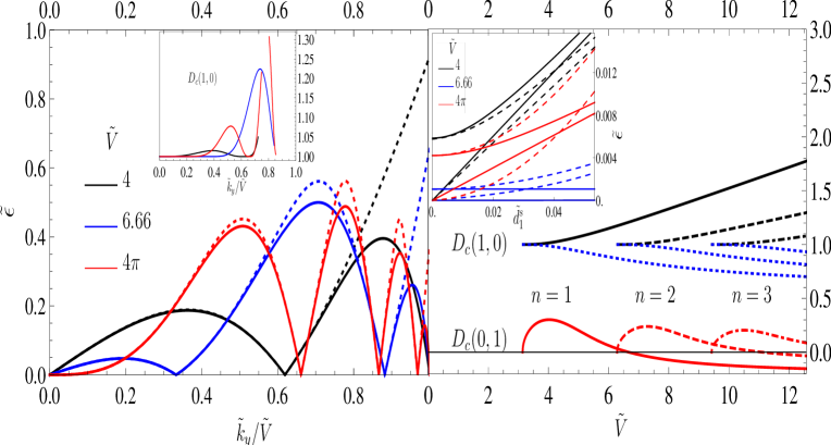
Figure 1: Left panel: Energy spectrum $\epsilon^{0}_{+}$ (12) at $\tilde{k}_{x}=0$ and $\tilde{\mu}=0$, $s=1$ for various SL potentials $\tilde{V}$. Dotted curves show the corresponding exact spectrum obtained by evaluating the transfer matrix eigenvalue equation (10) numerically. Inset shows $D_{c}(1,0)$ (23) as a function of $\tilde{k}_{y}/\tilde{V}$ for $\epsilon^{0}=0$ and SL potentials $\tilde{V}=4,6.66,4\pi$. The curves are calculated by using the outer valley VHS chemical potentials $\tilde{\mu}=0.185,0.5$ in the case $\tilde{V}=4,6.66$, and by using the average chemical potential of the three existent VHSs $\tilde{\mu}=0.415$ being of similar absolute energy value for $\tilde{V}=4\pi$. Right panel: $D_{c}(1,0)$ and $D_{c}(0,1)$ for $\epsilon^{0}=0$, $k_{y}=k_{y}^{n}$ and chemical potentials $\tilde{\mu}$ at the VHSs $n=1,\ldots,3$ where $n=1$ corresponds to the outermost VHS. The dotted curves show $D_{c}(1,0)$ by going one order higher taking into account (13) up to order $(\tilde{E}\tilde{V}/\alpha_{0})^{2}$. $D_{c}(0,1)$ is not changed within this approximation. Inset shows the energy spectrum $\tilde{\epsilon}_{+}$ (22) for $d_{1}^{c}=0$ as a function of $\tilde{d}_{1}^{s}$ for $\epsilon^{0}=0$ and also one further value $\epsilon^{0}\not=0$. The specific value can be read off from the intersection of the spectral curve with the $y$-axis. The corresponding dashed curves are calculated by a numerical diagonalization of (2) using a transfer matrix method similar to (5)–(10).

Until now, we have only discussed the $d_{1}$-dependence of the energy spectrum. From Eq. (19), we obtain that close to a VHS for pure condensates, i.e. where $d_{i}\not=0$ for only one $i$ and the rest of the condensates is zero, only the $d_{3}$ beside the $d_{1}$ condensate has a nonzero contribution in the gap function $D$. The $d_{2}$-dependence in the gap function comes in via $\Lambda^{2}_{ij}$, leading to mixing terms of the pure condensate contributions to the gap function. That the $d_{4}$-condensate does not contribute to the gap function is caused by the fact that $\hat{{\bf\Delta}}_{\pm V}$ does not depend on $d_{4}$.

For the $d_{3}$ dependence of the energy gap function $D$, i.e. by setting $d_{i}=0$ for $i\not=3$, we obtain the expression (23) with the substitutions $d_{1}^{c}\rightarrow d_{3}^{s}$, $d_{1}^{s}\rightarrow d_{3}^{c}$, and after a multiplication of a reduction factor $\tilde{k}_{y}/\tilde{V}$. The reduction factor has its origin in the prefactor differences between $\Lambda^{1}_{31}$ and $\Lambda^{1}_{32}$ (19). In general, we obtain for the energy spectrum (22) in the relevant large energy regime $|\tilde{\epsilon}^{0}|\gg{\rm max}[|\tilde{d}_{i}|]$ for superconductivity $D^{2}=D^{2}_{c,i}$ where

$$D^{2}_{c,i}=D^{2}_{c}(d_{1}^{c},d_{1}^{s})+\frac{\tilde{k}^{2}_{y}}{\tilde{V}^{2}}D^{2}_{c}(d_{3}^{s},d_{3}^{c})$$ (24)

$$\qquad-2\frac{\tilde{k}_{y}}{\tilde{V}}D_{c}(d_{1}^{c},d_{1}^{s})D_{c}(d_{3}^{s},d_{3}^{c})\frac{2{\rm Im}[EV_{i}]}{1+|EV_{i}|^{2}}\,,$$

and $i=1,2$. Here we denoted by $(1,EV_{i})^{T}$ for $i=1,2$ as the eigenvectors of the matrix $\Lambda^{2}_{ij}$ for $i,j\in\{1,2\}$ and $EV_{i}$ is a function of the condensates $d_{1},d_{2}$, and $d_{3}$. In the less relevant regime $|\tilde{\epsilon}^{0}|\ll{\rm max}[|\tilde{d}_{i}|]$, the gap function $D$ looks similar where $2{\rm Im}[EV_{i}]/(1+|EV_{i}|^{2})=\pm 1$. We now obtain from (24) that the degeneracy of the energy spectrum seen for the pure $d_{1}$ condensates in (22) with (23) is lifted.

IV BCS-instability

We are now able to calculate from the one-particle spectrum (22) the $\Delta$-dependent part of the grand canonical potential $\tilde{\Omega}$. The condensates $d_{i}$ are then determined by minimizing $\tilde{\Omega}$ with respect to the pair functions $d_{i}^{s},d_{i}^{c}$. We restrict our search of the minimum thereby by comparing the minimum of the free energies in the various basic directions where $d_{i}\not=0$ for one $i$ but zero for the others. This restriction is justified by taking into account the the smallness of the condensate mixing term in Eq. (24) and further that the energy regime $|\tilde{\epsilon}^{0}|\gg{\rm max}[|d_{i}|]$ in the spectrum gives the dominant contribution to the free energy integral in the weak coupling regime (see the discussions below). For the mixing last term in (24) we mention that $2{\rm Im}[EV_{i}]/(1+|EV_{i}|^{2})\leq 1$ is strongly dependent on the momenta and condensate values $d_{1},d_{2},d_{3}$. For a justification of its smallness one can show that $2{\rm Im}[EV_{i}]/(1+|EV_{i}|^{2})$ is zero for $d_{2}=0$ and becomes much smaller than one at least for one $EV_{i}$ in the regime where $d^{c}_{1}\sim d_{3}^{s}\gg d^{s}_{1},d^{c}_{3}$.

When considering only the large energy regime together with the neglecting of the mixing term, our restricted minimum search in the free energy is then even exact. Due to the additional small prefactor $\tilde{k}_{y}/\tilde{V}$ of the condensate contributions of $d_{3}$ in comparison to $d_{1}$ in the energy gap $D$ the condensate $d_{1}\not=0$ leads to a smaller free energy than the other condensates. This results in the free energy

$$\tilde{\Omega}\frac{d^{2}}{S}\!=\!-\frac{32\tilde{T}}{(2\pi)^{2}}\frac{1}{\hat{\alpha}^{4}_{0}}\!\!\!\!\!\!\!\!\!\!\int\limits_{0}^{\sqrt{\tilde{V}^{2}-(\pi/2)^{2}}}\!\!\!\!\!\!\!\!\!\!d\tilde{k_{y}}\int\limits_{-\tilde{\omega}_{DB}^{*}}^{\tilde{\omega}^{*}_{DB}}\!\!\!\!d\tilde{\epsilon}^{0}_{+}\bigg{\{}\Theta(\pi/2-\tilde{k}_{x}^{+})\frac{|\tilde{E}_{+}|}{\tilde{k}_{x}^{+}}$$

$$\times\log\left[2+2\cosh\left(\frac{\tilde{\epsilon}_{+}}{\tilde{T}}\right)\right]\bigg{\}}+\frac{16}{\tilde{g}}\,[(\tilde{d}_{1}^{c})^{2}+(\tilde{d}_{1}^{s})^{2}]\,$$ (25)

where $\tilde{g}=2g/d\hbar v_{F}$. The condensate values $d_{1}^{c}$, $d_{1}^{s}$ are then determined by minimizing $\tilde{\Omega}$. We show in Fig. 2 the resulting $d_{1}^{c}$, $d_{1}^{s}$ values as a function of the dimensionless temperature $\tilde{T}$ for various SL potentials $\tilde{V}$. The dimensionless effective Debye frequency is given by $\tilde{\omega}_{\rm DB}^{*}\approx 0.017\tilde{V}{\rm min}[d/a\tilde{V},1]$. In Kelvin we obtain, assuming a maximal longitudinal acoustic phonon frequency in graphene of $\omega_{\rm DB}\approx 1960K$, $\omega_{\rm DB}^{*}\approx 1960{\rm K}\cdot{\rm min}[\tilde{V}a/d,1]$. From Fig. 1 we obtain that the highest critical temperatures $T_{c}$ are gained for large $\tilde{V}$. For $\tilde{V}=4\pi$, ($\tilde{V}=6.66$), (($\tilde{V}=4$)) we obtain $T_{c}=\{1136{\rm K},315{\rm K},58{\rm K}\}$ ($\{587{\rm K},104{\rm K},9{\rm K}\}$) (($\{76{\rm K},2.5{\rm K},0.154{\rm K}\}$)) at $d/a=\{8,16,32\}$. We find further $\tilde{T}_{c}/\tilde{\omega}_{\rm DB}^{*}=\{0.58,0.205,0.075\}$, ($\{0.36,0.13,0.02\}$), (($\{0.078,0.005,0.0006\}$)) and $\tilde{d}^{c}_{1}/\tilde{\omega}_{\rm DB}^{*}\approx\{1.06,0.35,0.1\}$, ($\{0.62,0.21,0.017\}$), (($\{0.13,0.0196,0.0011\}$)) at $T=0$. It is well known that due to decoherence effects of the electronic wavefunction for $T_{c}/\omega_{\rm DB}^{*}\gtrsim 1$ and the neglection of retardation in the Fröhlich Hamiltonian for $d_{1}/\omega_{\rm DB}^{*}\gtrsim 1$, the BCS results cannot be trusted any longer in this regime. The regime is commonly called the intermediate to strong-coupling regime. $T_{c}$ as well as $d_{1}$ are then truncated at $\omega_{\rm DB}^{*}$ Alexandrov1 . A better description in this regime takes into account higher order fluctuation effects as well as the frequency dependence of the effective electron-electron interaction being described by Eliashberg theory in the intermediate coupling regime and polaron superconductivity for strong couplings Alexandrov1 . The results in both regimes for metals as well as for pristine graphene within Eliashberg theory Einenkel1 suggest that a realistic cut-off for $T_{c}$ should be in the vicinity of $\omega_{\rm DB}/3$, leading to $T_{c}$ values up to $650{\rm K}$.

The analysis in this paper is based on the effective mass approximation (1) for the graphene Hamiltonian. This approximation is justified in the case of the linearity of the graphene spectrum. The linearity is fulfilled in first approximation for momenta $|{\bf k}|\lesssim k_{\rm BZ}/2$ around the ${\bf K}$, $-{\bf K}$ points. The relevant $k_{y}$-momentum of a saddle point of a VHS calculated by (1) should then lie in this momentum regime. This regime is roughly fulfilled for the parameters of the SL potentials shown in Fig. 2. We point out that the whole analysis in the last two sections is mainly based on the folding behavior of the energy band. This behavior is a much more stable property with respect to perturbations of the graphene lattice than for example the creation of new Dirac points. This justifies further the use of the effective mass approximation for VHSs with saddle points at large effective momenta.

In the low coupling regime ($T_{c}\ll W$), we obtain from (25) by using (14)

$$\log^{2}\left(\frac{\tilde{W}^{2}_{\rm VHS}}{\tilde{T}_{c}|\tilde{\mu}|/2}\right)-\log^{2}\left(\frac{\tilde{W}^{2}_{\rm VHS}}{\tilde{W}|\tilde{\mu}|/2}\right)\approx\frac{16}{\tilde{\nu}_{0}\tilde{g}}\frac{1}{\|D_{c}\|^{2}}\,,$$ (26)

where $\tilde{W}$ is the effective band width $\tilde{W}={\rm min}[\tilde{\omega}_{\rm DB}^{*},\tilde{W}_{\rm VHS}]$ and $\left\|D_{c}\right\|\equiv\sqrt{D_{c}(1,0)^{2}+D_{c}(0,1)^{2}}$ calculated with the saddle point momentum $k_{y}=k_{y}^{n}$. The condensates $\tilde{d}_{1}^{c}$, $\tilde{d}_{1}^{s}$ at $T=0$ in the low-coupling regime are given by

$$\tilde{d}^{c}_{1}=D_{c}(1,0)\|\tilde{d}_{1}\|/\|D_{c}\|,\tilde{d}^{s}_{1}=D_{c}(0,1)\|\tilde{d}_{1}\|/\|D_{c}\|\,.$$ (27)

Here $\|\tilde{d}_{1}\|$ is given by (26) with the substitution $2\tilde{T}_{c}\rightarrow\|D_{c}\|\|\tilde{d}_{1}\|$. In the strong coupling regime $\tilde{W}$ replaces $\tilde{\omega}_{\rm DB}^{*}$ as a cut-off for $\tilde{T}_{c}$ and $\|\tilde{d}_{1}\|$ for $T=0$.

From (26), (27), we obtain then that in leading order $d^{s}_{1}/d^{c}_{1}\approx D_{c}(0,1)/D_{c}(1,0)$ calculated for $k_{y}=k_{y}^{n}$ at $T=0$. This is qualitatively in accordance to Fig. 2 by using the results for $D_{c}(0,1)$, $D_{c}(1,0)$ in Fig. 1. By this we mean that $d^{s}_{1}/d^{c}_{1}$ is much larger for $\tilde{V}=4$ in comparison to $\tilde{V}=4\pi$, $6.66$. Nevertheless we obtain quantitatively discrepancies which are attributed to contributions in the gap equation (25) which are not taken into account by the VHS contribution (26). For a justification we mention that $D_{c}(0,1)/D_{c}(1,0)$ is oscillatory as a function of $k_{y}$. For example for $\tilde{V}=4$ we obtain that $D_{c}(0,1)/D_{c}(1,0)\approx 0.3$ at $k_{y}=k_{y}^{1}$. This is almost the maximum value of $D_{c}(0,1)/D_{c}(1,0)$ as a function of $k_{y}$, showing even negative values $D_{c}(0,1)/D_{c}(1,0)\approx-1$ for larger $k_{y}$.

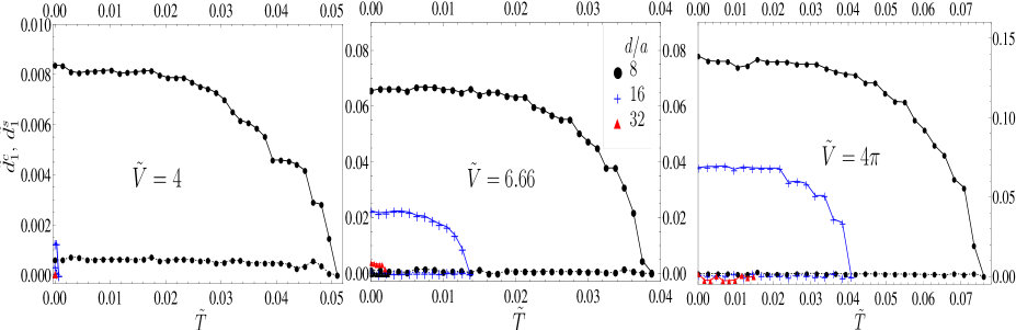
Figure 2: We show the condensate quantities $\tilde{d}^{c}_{1}$ (upper solid curves) and $\tilde{d}^{s}_{1}$ (lower dotted curves) for various SL potentials $\tilde{V}$ as a function of temperature by minimizing the free energy (25). The chemical potentials are chosen to lie at the outer valley VHSs for $\tilde{V}=4,6.66$ and at the average of the VHS energies for $\tilde{V}=4\pi$ (see caption to Fig. 1)

Finally we compare our results with the phonon mediated superconductivity in pristine graphene without an SL. We shall calculate in the following $T_{c}$ for acoustic phonon pairing and in a rough approximation also for optical phonon pairing in order to demonstrate the proportion of the critical temperatures for both pairing mechanisms. We restrict ourselves hereby to the $d^{c}_{1}$ pairing mechanism which leads to

$$\log\left(\frac{\hbar\omega^{p}_{\rm DB}}{T_{c}}\right)\approx 2\frac{1}{g_{p}\nu_{p}(\mu)}\,.$$ (28)

The cut-off frequency $\omega^{p}_{\rm DB}$ is given by $\omega^{p}_{\rm DB}\approx\omega_{\rm DB}$ for optical phonon pairing and $\omega^{p}_{\rm DB}\approx(|\mu|/\hbar v_{F}k_{\rm DB})\omega_{\rm DB}$ for acoustic phonon pairing. For the former we use that the acoustic Debye frequency and the optical phonon frequencies are of similar value in graphene Suzuura1 . The density of states $\nu_{p}(\mu)$ per spin and valley for pristine graphene is given by $\nu_{p}(\mu)=|\mu|/2\pi(\hbar v_{F})^{2}$. The constant $g_{p}$ in (28) is the effective Fröhlich interaction constant being $g_{p}=g\approx 6\cdot 10^{-19}m^{2}{\rm eV}$ for acoustic phonon pairing and $g_{p}\approx 7.02\cdot 10^{-20}m^{2}{\rm eV}$ for pairing with optical phonons Calandra2 . The factor two on the right-hand side of Eq. (28) is attributed to the chiral nature of the graphene lattice with two atoms in the fundamental cell where for large chemical potentials only electrons in one of the bands $\pi^{*}$ or $\pi$ with energies close to the chemical potential can pair. The maximal absolute electron density which can be reached by electrostatic doping till now leading to the highest $T_{c}$ values is given by $n_{e}\approx 4\cdot 10^{14}cm^{-2}$ Efetov1 . By using (28) for this density we obtain $T_{c}\approx 4.1\cdot 10^{-3}\omega_{\rm DB}\approx 8{\rm K}$ for acoustic phonon coupling (here $|\mu|/\hbar v_{F}k_{\rm DB}\approx 1/5$) and $T_{c}\approx 2.7\cdot 10^{-15}\omega_{\rm DB}\approx 5.4\cdot 10^{-12}{\rm K}$ for optical phonons. These transition temperatures are much smaller than most of the transition temperatures in graphene superimposed by an SL with parameters used in Fig. 2.

Until now, we have restricted our minimum search of the free energy to condensates of the form (4) showing the full symmetry of the SL together with the time inversion symmetry and spin singlet form. In general the condensate matrix $\Delta$ has no restrictions from the beginning. The BdG Hamiltonian (2) shows an independent chiral symmetry in the electronic and hole sector. We are justifying in App. A the utilized condensates (4) by showing that the condensate $d_{1}^{c}$ modulo its chiral symmetric counterparts, i.e. $\Delta\rightarrow(U_{1}^{+}\otimes\sigma_{0})\Delta(U_{2}\otimes\sigma_{0})$ where $U_{1},U_{2}$ are arbitrary constant unitary $2\times 2$ matrices and $\Delta=\Delta_{1}$, have the largest condensate values together with the minimal free energy and dominate the BCS pairing process. We use hereby as was implicitly also used above that the Fröhlich coupling constant $g$ for acoustic phonons is not depending on the pairing deduced from $H_{\rm ep}$. This is not fulfilled for other coupling mechanisms as for example the coupling with optical phonons. A benefit of the analysis used in App. A is that it can be simply adapted to other coupling mechanisms.

It is well known that in two dimensions the phase fluctuations of a continuous order parameter are so strong that a finite order parameter value calculated in mean-field vanishes in higher order approximations (Hohenberg-Mermin-Wagner-Theorem). Nevertheless a finite expectation value for the amplitude of the order parameter is still possible. At lower temperatures where the order parameter amplitude is non-zero a Kosterlitz-Thouless transition emerges which is connected to an unbinding of vortex-antivortex excitations when crossing the temperature from below Kleinert1 ; Minnhagen1 . The free vortices prohibit then in the so called pseudo-gap phase that a true superconductivity behavior is existent. At lower temperatures where the vortices are bound, we can find in two-dimensional systems superconductivity. In other words, the mean-field BCS theory which we formulated in this paper, approximatively can only describe the transition temperature where the pairing amplitude is unequal to zero being then an upper bound for the true superconducting phase transition temperature. This temperature difference where the order parameter amplitude becomes unequal to zero and where the vortex unbinding happens is not large at least in the regime where $\mu\gg\omega_{\rm DB}$ was shown quantitatively in the case of two-dimensional metals in Refs. Loktev1, ; Loktev2, by using Eliashberg theory. Due to this, we also expect in the case of the graphene system that the two temperatures are quite close to each other.

V Summary

We have examined possible BCS instabilities mediated by acoustic ${\bf\Gamma}$ phonons in electrical superlattice systems. Here we restrict ourselves to SL potentials $\tilde{V}\gtrsim 1$, $d/a\gg 1$ where $\tilde{V}a/d$ is not too small such that the acoustic phonon coupling is in fact the dominating phonon coupling process. In the regime $\tilde{V}\gtrsim 1$, the energy bands are folded where new Dirac points linked by low-lying energy VHSs emerge. We considered in this paper mainly pairing for chemical potentials close to VHSs where the highest $T_{c}$ temperatures are attained. For SL systems such chemical potentials should be reached by electrostatic doping. We showed under the assumption of a pairing that fulfills time inversion symmetry together with the symmetry of the SL and graphene lattice that electronic onsite s-wave pairing of an electron around the ${\bf K}$ point with another electron around the $-{\bf K}$ point is most relevant. The relevant order parameter is almost constant in space. We obtain large transition temperatures $T_{c}$ especially where VHSs lie close to each other. We have compared the calculated $T_{c}$ values of the SL system with phonon mediated transition temperatures of electrostatic doped pristine graphene. Finally, we argued that the encountered order parameter (up to chiral symmetry) is also the leading electronic pairing mechanism when taken into account no symmetry restrictions on the condensate matrix.

We have used in this paper the simplest theory for superconductivity appropriate for pairing in the low coupling limit for electrons around the ${\bf K}$, $-{\bf K}$ points. Our examples in Fig. 2 produce superconductivity at rather high temperatures, and at the highest $T_{c}$ values the system parameters lies at the validity boundary of the model. In this case, the calculated $T_{c}$-values are only a rough approximation for the experimental transition temperatures where more exact calculations would be useful by using for example the full tight binding Hamiltonian together with Eliashberg theory for the SL superimposed graphene system.

Appendix A The dominance of $d^{c}_{1}$ condensates and its chiral equivalences among general condensates

In the main text we considered only highly symmetric condensates as possible electron pairings which fulfill the full mirror symmetry of the SL and additional time inversion symmetry and spin singlet pairing. This led to the condensates (4) as the only contributions to the matrix $\Delta$. As was mentioned in the main text, we have in general no restriction for acoustic phonon coupling on the condensate matrix $\Delta$. In the following we shall use again the approximation that the matrix is step-like in space meaning that it is constant for constant $V(x)$. In weak-coupling BCS physics, the regime $|\epsilon^{0}_{\pm}|\gg{\rm max}[|\Delta_{ij}|]$ of the spectrum is most relevant for superconducting pairing. Let us recall from the main text in Sect. III that in the case of the highly symmetric condensates, the dominance of the $d^{c}_{1}$-condensate contributions over the $d^{s}_{1}$- and $d_{3}$-contributions came mainly from the fact that in the gapfunction $D_{c}$ (23) the prefactor $\sim A^{2}+B^{2}$ for $d_{1}^{c}$ is much larger than the prefactor $\sim AB$ for $d_{1}^{s}$. Furthermore we found the dominance of the $d_{1}$ condensates over the $d_{3}$ condensates due to an additional prefactor $\tilde{k}_{y}/\tilde{V}$ in the $d_{3}$ condensate term (24).

These prefactors were calculated by using (17) with (13). Within a similar argument we obtain that the dominant contributions for general $\Delta_{ij}$ are given by $\Delta^{d}=\sum^{3}_{i=0}do_{i}\sigma_{i}\otimes\sigma_{0}$. The condensates $do_{i}$ are in general complex and constant over the whole SL. Other condensates of the matrix form $\sum^{3}_{i=0}do_{i}\sigma_{i}\otimes\sigma_{1}$ and $\sum^{3}_{i=0}do_{i}\sigma_{i}\otimes\sigma_{3}$ lead to energy gap contributions being a factor $AB/(A^{2}+B^{2})$ smaller where condensates of the form $\sum^{3}_{i=0}do_{i}\sigma_{i}\otimes\sigma_{2}$ are a factor $\tilde{k}_{y}/\tilde{V}$ smaller.

By using the chiral invariance of (2) in the electron and hole sector independently we can restrict ourselves by using the singular value decomposition of the matrix $\Delta^{d}$ to matrices $\Delta^{d}=do^{r}_{1}(\sigma_{3}+\sigma_{0})/2\otimes\sigma_{0}+do^{r}_{2}(\sigma_{3}-\sigma_{0})/2\otimes\sigma_{0}$. Here $do^{r}_{1}$ and $do^{r}_{2}$ are real condensates being constant over the SL. The dominant mass gap contributions $D=D^{d}_{c,i}$ are then given by

$$D^{d}_{c,i}=D_{c}(1,0)\sqrt{\frac{(do^{r}_{1})^{2}+|EV_{2}|^{2}(do^{r}_{2})^{2}}{1+|EV_{2}|^{2}}}\,.$$ (29)

Here $(1,EV_{1})^{T}$, $(1,EV_{2})^{T}$ are the two orthogonal eigenvectors of the matrix $\Lambda^{2}_{ij}=\langle u^{0}\otimes e_{i}|{\bf\Lambda}^{2}(d)|u^{0}\otimes e_{j}\rangle_{Q}$ for $i,j=1,2$ in the electronic sector where now also contributions from smaller subleading condensate contributions can have a strong influence via $EV_{i}$ on the free energy. For deriving (29) we took into account the discussion following (19). Note that the spectrum (29) with (22) for $D=D^{d}_{c,1}$ and $D=D^{d}_{c,2}$, respectively, is now in general no longer degenerate as in (20)-(23) but has two nondegenerate bands with two different gap values. We now minimize the dominant part of the free energy first with respect to $EV_{1},EV_{2}$. The $EV_{i}$-dependence comes then in only via the first term in (25) where now we have to substitude $\log[2+2\cosh(\tilde{\epsilon}_{+}/\tilde{T})]$ by $\sum_{i}\log[2+2\cosh(\tilde{\epsilon}^{i}_{+}/\tilde{T})]/2$. Here $\tilde{\epsilon}^{i}_{+}$ is defined via (22) using (29) with the substitution $D^{d}_{c,i}$ for $D$ . By using the concavity of $\log[2+2\cosh(\sqrt{(\epsilon^{0}_{+})^{2}+x}/\tilde{T})]$ as a function of $x$, and further that $(D^{d}_{c,1})^{2}+(D^{d}_{c,2})^{2}$ does not depend on $EV_{1}$ and $EV_{2}$ we obtain that the minimal free energy is attained for $|EV_{1}|=|EV_{2}|=1$. The dominant contribution to the free energy $\tilde{\Omega}^{d}$ is then given by (25) with the substitutions above where we further have to substitude $(\tilde{d}^{c}_{1})^{2}+(\tilde{d}^{s}_{1})^{2}$ by $((\tilde{do}^{r}_{1})^{2}+(\tilde{do}^{r}_{2})^{2})/2$. This free energy shows a $O(2)$ invariance. By choosing $do^{r}_{1}=-do^{r}_{1}$ we obtain exactly the $d^{c}_{1}$-contribution to the condensate matrix (4).

References

- (1) V. I. Talyanskii, D. S. Novikov, B. D. Simons, and L. S. Levitov, Phys. Rev. Lett. 87, 276802 (2001).
- (2) L. Brey and H. A. Fertig, Phys. Rev. Lett. 103, 046809 (2009).
- (3) C.-H. Park, Y.-W. Son, L. Yang, M. L. Cohen, and S. G. Louie, Phys. Rev. Lett. 103, 046808 (2009).
- (4) C.-H. Park, L. Yang, Y.-W. Son, M. L. Cohen, and S. G. Louie, Phys. Rev. Lett. 101, 126804 (2008).
- (5) C.-H. Park, Y.-W. Son, L. Yang, M. L. Cohen, and S. G. Louie, Nano Lett. 8, 2920 (2008).
- (6) I. Pletikosić, M. Kralj, P. Pervan, R. Brako, J. Coraux, A. T. N’Diaye, C. Busse, T. Michely, Phys. Rev. Lett. 102, 056808 (2009).
- (7) M. Yankowitz, J. Xue, D. Cormode, J. D. Sanchez-Yamagishi, K. Watanabe, T. Taniguchi, P. Jarillo-Herrero, P. Jacquod, and B. J. LeRoy, Nat. Phys. 8, 382 (2012).
- (8) H. Yan, Z. -D. Chu, W. Yan, M. Liu, L. Meng, M. Yang, Y. Fan, J. Wang, R.-F. Dou, Y. Zhang, Z. Liu, J.-C. Nie, and L. He, Phys. Rev. B 87, 075405 (2013).
- (9) J. Dietel and H. Kleinert, Phys. Rev. B 84, 121404(R) (2011).
- (10) J. Dietel and H. Kleinert, Phys. Rev. B 86, 115450 (2012).
- (11) P. Burset, A. L. Yeyati, L. Brey, and H. A. Fertig, Phys. Rev. B 83, 195434 (2011).
- (12) J. Sun, H. A. Fertig, and L. Brey, Phys. Rev. Lett. 105, 156801 (2010).
- (13) M. Barbier, P. Vasilopoulos, F. Peeters, Phil. Trans. R. Soc. A 368, 5499 (2010).
- (14) T. E. Weller, M. Ellerby, S. S. Saxena, R. P. Smith, and N. T. Skipper, Nat. Phys. 1, 39 (2005).
- (15) M. Calandra and F. Mauri, Phys. Rev. Lett. 95, 237002 (2005).
- (16) O. Gunnarson, Rev. Mod. Phys. 69 225 (2005).
- (17) A. S. Alexandrov, Theory of Superconductivity, (IOC Publishing Ltd 2003, Bristol and Philadelphia).
- (18) P. Morel and P. W. Anderson, Phys. Rev. 125, 1263 (1962).
- (19) M. Sigrist, AIP Conf. Proc. 789, 165 (2005).
- (20) H. A. Castro Neto, F. Guinea, N. M. R. Peres, K. S. Novoselov and A. K. Geim, Rev. Mod. Phys. 81, 109 (2009).
- (21) C. M. Varma, J. Zaanen, and K. Raghavachari, Science 254, 989 (1991).
- (22) J. Eisenstein, Rev. Mod. Phys. 26, 277 (1954).
- (23) G. Savini, A. C. Ferrari, F. Giustino, Phys. Rev. Lett. 105, 037002 (2010).
- (24) N. B. Kopnin, T. T. Heikkilä, and G. E. Volovik, Phys. Rev. B 83, 220503(R) (2011).
- (25) B. Uchoa and Y. Barlas, Phys. Rev. Lett. 111, 046604 (2013).
- (26) B. Uchoa and A. H. Castro Neto, Phys. Rev. Lett. 98, 146801 (2007).
- (27) N. B. Kopnin and E. B. Sonin, Phys. Rev. Lett. 100, 246808 (2008).
- (28) M. Einenkel, K. Efetov, Phys. Rev. B 84, 214508 (2011).
- (29) H. Suzuura and T. Ando, J. Phys. Soc. Jap. 77, 044703 (2008).
- (30) K. Ishikawa and T. Ando, J. Phys. Soc. Jap. 75, 084713 (2006).
- (31) S. Pisanec, M. Lazzeri, F. Mauri, A. C. Ferrari, and J. Robertson, Phys. Rev. Lett. 93, 185503 (2004).
- (32) J. Dietel and H. Kleinert, Phys. Rev. B 82, 195437 (2010).
- (33) D. K. Efetov, P. Kim, Phys. Rev. Lett. 105, 256805 (2010).
- (34) J. Gonzáles, Phys. Rev. B 78, 205431 (2008).
- (35) R.Ñandkishore, L. S. Levitov, and A. V. Chubokov, Nat. Phys. 8, 158 (2012).
- (36) M. L. Kiesel, C. Platt, W. Hanke, D. A. Abanin, R. Thomale, Phys. Rev. B 86, 020507(R) (2012).
- (37) J. L. McChesney, A. Bostwick, T. Ohta, T. Seyller, K. Horn, J. Gonzáles, and E. Rotenberg, Phys. Rev. Lett. 104, 136803 (2010).
- (38) J. Dietel and H. Kleinert, Phys. Rev. B 79, 075412 (2009).
- (39) D. P. Arovas, L. Brey, H. A. Fertig, E. -A. Kim, and K. Ziegler, New Journal of Physics 12, 123020 (2010).
- (40) M. Barbier, P. Vasilopoulos, and F. M. Peeters, Phys. Rev. B 81, 075438 (2010).
- (41) M. Calandra and F. Mauri, Phys. Rev. B 76, 205411 (2007).
- (42) H. Kleinert, Gauge Fields in Condensed Matter: vol. I Superflow and Vortex Lines, (World Scientific 1989, Singapore)
- (43) P. Minnhagen, Rev. Mod. Phys. 59, 1001 (1987).
- (44) V. M. Loktev, S. G. Sharapov and V. M. Turkovski, Physica C 296, 84 (1998).
- (45) V. M. Loktev, and V. M. Turkovski, JETP 87, 329 (1998).