Suppression of the quantum collapse in binary bosonic gases

Abstract

Attraction of the quantum particle to the center in the 3D space with potential $-V_{0}r^{-2}$ gives rise to the quantum collapse, i.e., nonexistence of the ground state (GS) when the attraction strength exceeds a critical value [$\left(V_{0}^{(\mathrm{cr})}\right)_{1}=1/8$, in the present notation]. Recently, we have demonstrated that the quantum collapse is suppressed, and the GS is restored, if repulsive interactions between particles in the quantum gas are taken into account, in the mean-field approximation. This setting can be realized in a gas of dipolar molecules attracted to the central charge, with dipole-dipole interactions taken into regard too. Here we analyze this problem for a binary gas. GSs supported by the repulsive interactions are constructed in a numerical form, as well as by means of analytical approximations for both miscible and immiscible binary systems. In particular, the Thomas-Fermi (TF) approximation is relevant if $V_{0}$ is large enough. It is found that the GS of the miscible binary gas, both balanced and imbalanced, features a weak phase transition at another critical value, $\left(V_{0}^{(\mathrm{cr})}\right)_{2}=1/2\equiv 4\left(V_{0}^{(\mathrm{cr})}\right)_{1}$. The transition is characterized by an analyticity-breaking change in the structure of the wave functions at small $r$. To illustrate the generic character of the present phenomenology, we also consider the binary system with the attraction between the species (rather than repulsion), in the case when the central potential pulls a single component only.

I Introduction

Attractive potential $U(r)=-V_{0}r^{-2}$ plays a critical role for the effect of the quantum collapse (alias “fall onto the center”) in the three-dimensional (3D) space LL : If $V_{0}$ exceeds a critical value [it is $V_{0}^{(\mathrm{cr})}=1/8$ in the notation adopted below, see Eqs. (LABEL:GP)], the corresponding 3D Schrödinger equation fails to produce the ground state (GS) (loosely speaking, in this case the energy of the GS collapses to $E\rightarrow-\infty$). This critical feature is explained by the fact that the quantization breaks the scaling invariance of the classical counterpart of the present quantum setting. The effect is also known as the quantum anomaly, alias “dimensional transmutation” anomaly .

A solution of the problem of the missing GS was elaborated in terms of the linear quantum field theory, which, by means of the renormalization procedure, postulated the existence of the GS, with an arbitrary spatial size anomaly . A different approach was recently proposed in our work we1 , which considered, in terms of the mean-field approximation, a bosonic gas (rather than the single particle) pulled to the center by potential $-V_{0}r^{-2}$, and took into regard the collision-induced repulsive nonlinearity in the corresponding Gross-Pitaevskii equation (GPE) Pit . The physical realization of the setting is possible in ultra-cold gases of molecules carrying a permanent electric dipole moment, $d$ (such as LiCs LiCs and KRb KRb ), which are attracted by electric charge $Q$ placed at the center (it may be an ion held by an optical trapping potential ion ). In this case, the attraction constant is

$$V_{0}=|Q|d.$$ (1)

Alternatively, it is possible to use an atomic gas in a long-lived excited state (such as a “frozen” low-lying Rydberg state Rydberg ; Rydberg-review , in which the permanent dipole moment grows with the principal quantum number, $n$, as $n^{2}$); to additionally stabilize the gas of excited atoms, one may pump it by a resonant laser field Rydberg-pump . The analysis reported in Ref. we1 took into account the dipole-dipole interaction in the gas too, also in the framework of the mean-field approximation, which amounts to an effective renormalization (increase) of the strength of the contact nonlinearity. As a result, it has been demonstrated that the repulsive nonlinearity suppresses the quantum collapse at all values of $V_{0}$, restoring the GS. An estimate with relevant values of physical parameters demonstrates that the radius of the resurrected GS may be a few $\mathrm{\mu}$m. In Ref. we2 , the analysis was extended for the dipolar gas polarized by strong uniform dc field, with the spatial symmetry reduced from spherical to cylindrical.

In Ref. we1 , the same problem was considered in the two-dimensional (2D) geometry, where, in the framework of the linear Schrödinger equation, the attractive potential $-V_{0}r^{-2}$ leads to the collapse at any finite value of $V_{0}$. In addition to the above-mentioned physical implementations, the 2D gas subject to the action of this potential may be composed of polarizable atoms without a permanent dielectric moment, while an effective moment is induced in them by the electric field of a uniformly charged wire set perpendicular to the system’s plane Schmiedmayer1 , or with an effective magnetic moment induced by a current filament set in the perpendicular direction we1 . However, the cubic repulsive nonlinearity is too weak to suppress the quantum collapse in the 2D setting, only the quintic term (if it is physically relevant) being strong enough for that purpose we1 . Indeed, the experimental realization of the above-mentioned quasi-2D system of polarizable atoms attracted to the charged wire has demonstrated a collapse-like behavior Schmiedmayer2 . Furthermore, if a gas is tightly confined near the 2D plane by a strong trapping potential acting in the transverse direction, then, in the limit of large density, the underlying cubic nonlinearity is effectively transformed into that with power $7/3$ Delgado , which is still weaker. On the other hand, in the same limit the underlying quintic term will be transformed into one with power $11/3$, which is sufficient for the suppression of the quantum collapse and rebuilding of the GS.

The objective of the present work is to extend the analysis of the suppression of the quantum collapse for the binary gas, which combines the intra-species repulsion with the interaction between two species, the relative strength of the inter-species repulsion being $\gamma$, see Eqs. (LABEL:GP) below. It is well known that $\gamma$ can be adjusted by means of the Feshbach resonance controlled by external fields Feshbach1 ; Feshbach2 . This, in turn, allows one to switch the binary system between regimes of miscibility at $\gamma<1$ and immiscibility at $\gamma>1$ Mineev ; misc . The point of the miscibility-immiscibility transition may be shifted from $\gamma=1$ to $\gamma>1$ by external confinement Merhasin ; confinement , and by linear mixing between the species Merhasin ; linear-coupling , including the mixing which represents the effective spin-orbit coupling in binary condensates SO . The immiscibility leads to the phase separation of binary condensates and formation of domain walls in the 1D geometry DW . In 2D and 3D settings, domain walls often form circular or spherical shells, respectively shells .

In this  work, we construct spherically symmetric GSs pulled to the center by potential $-V_{0}r^{-2}$, which acts on both species, or a single one, in the binary quantum gas. The GSs are stabilized against the collapse by the repulsive nonlinearity (in the case when the single species carries the dipolar moment pulled to the central charge, the inter-species interaction must be attractive, corresponding to $\gamma<0$, rather than repulsive). The GSs are constructed in miscible and immiscible settings alike. In the case of the immiscibility, we could identify phase-separated structures in the form of spherically symmetric shells, but not sectors (e.g., for equal norms of the immiscible components, we have not found states in the form of two hemispheres separated by a flat domain wall). In the miscible binary gas, two critical values of $V_{0}$ are found. One is $\widetilde{V}_{0}^{(\mathrm{cr})}=1/2\equiv 4V_{0}^{(\mathrm{cr})}$ (recall $V_{0}^{(\mathrm{cr})}=1/8$ is the value at which the GS breaks down in the linear Schrödinger equation) in the balanced and imbalanced miscible gases alike, i.e., the gases with equal or different norms of the two components. At $V_{0}=1/2$, the coupled GPEs feature a breakup of the analyticity and a change in the structure of the GS wave function at $r\rightarrow 0$ (nevertheless, the GS exists equally well at $V_{0}<1/2$ and $V_{0}>1/2$). The imbalanced miscible gas (with $\gamma<1$) gives rise to an additional critical value,$~{}\mathcal{V}_{0}^{(\mathrm{cr})}=(1/2)\left(1+\gamma\right)/\left(1-\gamma\right)$, which we consider only briefly.

The rest of the paper is organized as follows. The  model is formulated in Section II, which also includes analysis of the asymptotic form of the wave functions. In section III, basic numerical results are reported for the miscible and immiscible settings, along with additional approximate analytical results, including the Thomas-Fermi (TF) approximation, which is relevant in the case of large $V_{0}$. In Section IV, we consider the system with the single component pulled to the center, and attractive, rather than repulsive, inter-species interaction ($\gamma<0$). The paper is concluded by Section V.

II Formulation of the model and analytical considerations

The self-repulsive binary condensate pulled to the center by the attractive potential is described by the coupled GPEs, written here in the scaled form,following Ref. we1 :

$$i\frac{\partial\phi_{1}}{\partial t} = -\frac{1}{2}\nabla^{2}\phi_{1}+(|\phi_{1}|^{2}+\gamma|\phi_{2}|^{2})\phi_{1}-\frac{V_{0}}{r^{2}}\phi_{1}~{},$$

$$i\frac{\partial\phi_{2}}{\partial t} = -\frac{1}{2}\nabla^{2}\phi_{2}+(\gamma|\phi_{1}|^{2}+|\phi_{2}|^{2})\phi_{2}-\frac{V_{0}}{r^{2}}\phi_{2}~{}$$

(in Ref. we1 , the strength of the attractive potential was defined as $U_{0}\equiv 2V_{0}$), where $\gamma$ is the relative strength of the inter-species repulsion, while coefficients of the self-repulsion are scaled to be $1$. Spherically symmetric stationary states with chemical potential $\mu_{n}$, $n=1,2$, are looked for as

$$\phi_{n}\left(r,t\right)=r^{-1}\chi_{n}(r)\exp\left(-i\mu_{n}t\right),$$ (3)

where $\chi_{n}(r)$ are real functions obeying the coupled equations,

$$\mu_{1}\chi_{1} = -\frac{1}{2}\chi_{1}^{\prime\prime}-\frac{V_{0}}{r^{2}}\chi_{1}+\left(\chi_{1}^{2}+\gamma\chi_{2}^{2}\right)\frac{\chi_{1}}{r^{2}},$$

$$\mu_{2}\chi_{2} = -\frac{1}{2}\chi_{2}^{\prime\prime}-\frac{V_{0}}{r^{2}}\chi_{2}+\left(\chi_{2}^{2}+\gamma\chi_{1}^{2}\right)\frac{\chi_{2}}{r^{2}}.$$

In terms of functions $\chi_{n}(r)$, the norms of the wave functions are

$$N_{n}\equiv\int\left|\phi_{n}(\mathbf{r})\right|d\mathbf{r}=4\pi\int_{0}^{\infty}\left[\chi_{n}(r)\right]^{2}dr,$$ (5)

and the average squared radial size of the trapped mode is

$$\left\langle r_{n}^{2}\right\rangle=\frac{\int_{0}^{\infty}\left[\chi_{n}(r)\right]^{2}r^{2}dr}{\int_{0}^{\infty}\left[\chi_{n}(r)\right]^{2}dr}.$$ (6)

An expansion of solutions to Eqs. (LABEL:stat) at $r\rightarrow 0$ is looked for as we1

$$\chi_{n}(r)=\chi_{n}^{(0)}\left[1-c_{n}^{(1)}r^{s/2}-c_{n}^{(2)}r^{s/2+2}+\cdots-d_{n}^{(1)}r^{2}-d_{n}^{(2)}r^{4}+\cdots\right],$$ (7)

with a positive power, $s>0$ (here, $c_{1}\neq c_{2}$ is possible, but power $s$ must be the same for $\chi_{1}$ and $\chi_{2}$). The terms $\sim c_{n}^{(1,2,...)}$ and $d_{n}^{(1,2,...)}$ are produced, respectively, by terms on the right- and left-hand sides of Eqs. (LABEL:stat). The leading-order (most singular) terms, $\sim r^{-2}$, produced by the substitution of ansatz (7) into Eqs. (LABEL:stat), lead to a system of algebraic relations for coefficients $\chi_{n}^{(0)}$:

$$\chi_{1}^{(0)}\left[\left(\chi_{1}^{(0)}\right)^{2}+\gamma\left(\chi_{2}^{(0)}\right)^{2}\right] = V_{0}\chi_{1}^{(0)},$$

$$\chi_{2}^{(0)}\left[\left(\chi_{2}^{(0)}\right)^{2}+\gamma\left(\chi_{1}^{(0)}\right)^{2}\right] = V_{0}\chi_{2}^{(0)}.$$

Obviously, Eqs. (LABEL:chichi) may have solutions of two types, corresponding to miscible and immiscible states, respectively:

$$\chi_{1}^{(0)} = \chi_{2}^{(0)}\equiv\chi_{\mathrm{misc}}^{(0)}=\sqrt{V_{0}/\left(1+\gamma\right)};$$ (9)

$$\chi_{1}^{(0)} \equiv \chi_{\mathrm{immisc}}^{(0)}=\sqrt{V_{0}},~{}\chi_{2}^{(0)}=0.$$ (10)

The miscible and immiscible states, which are defined by relations (9) and (10), are relevant strictly for $\gamma<1$ and $\gamma>1$, respectively. Our numerical analysis demonstrates that immiscible modes do not exist at $\gamma<1$, while miscible ones are completely unstable at $\gamma>1$. Thus, unlike other settings featuring the miscibility-immiscibility transitions Merhasin -SO , in the present situation the transition point undergoes no shift from $\gamma=1$.

In the miscible state, the substitution of ansatz (7) into Eqs. (LABEL:stat) identifies two independent next orders, past $r^{-2}$, in the expansion at $r\rightarrow 0$, namely, $r^{s/2-2}$ and $r^{0}$ (constant). These terms are produced, respectively, by the right- and left-hand sides of Eqs. (LABEL:stat), as said above. The analysis of the former order ($r^{s/2-2}$) yields power $s$,

$$s=1+\sqrt{1+16V_{0}},$$ (11)

with $c_{1}=c_{2}$ in Eq. (7), while coefficient $c_{1}$ itself remains indefinite, in terms of the asymptotic expansion at $r\rightarrow 0$. The consideration of the latter order ($r^{0}$) produces coefficients $d_{n}^{(1)}$ in Eq. (7):

$$d_{n}^{(1)}=\frac{\mu_{1}+\mu_{2}}{2\left(1-2V_{0}\right)}-\frac{(-1)^{n}\left(\mu_{1}-\mu_{2}\right)}{2\left(1-2V_{0}\frac{1-\gamma}{1+\gamma}\right)}.$$ (12)

Furthermore, exactly at the critical point, $\left(V_{0}^{(\mathrm{cr})}\right)_{2}=1/2$, at which the first term in expression (12) does not make sense, expansion (7) for the fully mixed state is replaced by

$$\chi_{n}(r)=\frac{1}{\sqrt{2\left(1+\gamma\right)}}\left[1+\frac{\mu_{1}+\mu_{2}}{4}r^{2}\ln\left(\frac{r_{0}}{r}\right)+(-1)^{n}\frac{1+\gamma}{4\gamma}\left(\mu_{1}-\mu_{2}\right)r^{2}\right],$$ (13)

where $r_{0}$ is an arbitrary scale constant, in terms of the expansion at $r\rightarrow 0$.

These results demonstrate the breakup of analyticity in the dependence of the GS wave function on $V_{0}$ at $V_{0}=1/2$. Indeed, at $V_{0}<1/2$, i.e., $s/2<2$ [see Eq. (11)] the expansion of the wave function at $r\rightarrow 0$ is dominated by terms $\sim r^{s/2}$, while at $V_{0}>1/2$ the power of the leading terms ($\sim r^{2}$) is fixed to be $2$, i.e., the non-analyticity is manifest in the dependence of the power of the leading term of the expansion on $V_{0}$. This conclusion is corroborated in Fig. 1 by shapes of functions $\chi(0)-\chi(r)\equiv\sqrt{V_{0}}-\chi_{1}(r)$, found from numerical solutions of Eq. (LABEL:stat) at $\gamma=0.9<1$ at different values of $V_{0}$. The power of the first correction to the constant term is given by the slope of the plots shown on the double-logarithmic scale in Fig. 1. The slope is indeed equal to $2$ at $V_{0}\geq 1/2$, taking smaller values at $V_{0}<1/2$. Note that at $V_{0}>1/2$ terms $\sim r^{s/2}$ in expansion (7), although they are no longer leading ones, are essential, as the free coefficient in front of them, $c_{1}=c_{2}$, is necessary to adjust the wave function to the condition of its exponential decay at $r\rightarrow\infty$, see Eq. (16) below.

Figure 1: Numerically found profiles of stationary wave functions for Eq. (4) are shown, in the form of $\chi(0)-\chi(r)$, where $\chi(0)=\sqrt{V_{0}}$ at $\gamma=0.9$ on the double-log scale for several values of $V_{0}$, below and above the weak-phase-transition-point, i.e, at $V_{0}<1/2$ and $V_{0}>1/2$, respectively. All the profiles are obtained for the same norm, $N_{1}=4\pi$.

Non-analyticity of structural and correlation functions is a characteristic feature of phase transitions in many-body settings, as shown in detail for the Calogero-Sutherland model Grisha and for many other systems nonanalytic , including, incidentally, binary fluids binary-fluid .Therefore, the analyticity breakup observed in the present model at $\left(V_{0}^{(\mathrm{cr})}\right)_{2}=1/2$ suggests that the model undergoes a phase transition at this point, although the GS exists equally well at $V_{0}<1/2$ and $V_{0}>1/2$. Recall that the onset of the quantum collapse in the linear version of the model occurs at the critical value $\left(V_{0}^{(\mathrm{cr})}\right)_{1}=1/8$ LL , which is a quarter of $\left(V_{0}^{(\mathrm{cr})}\right)_{2}$. In fact, this phase transition is a weak one, as the structural characteristic of the wave function which features the loss of the analyticity is a subtle one. Accordingly, it is shown below (see Fig. 6) that the transition can be seen in a subtle change of the experimentally observable dependence of the average radius of the ground state [Eq. (6)] on the attraction strength, $V_{0}$.

In the general case of the imbalanced miscible gas, with $\mu_{1}\neq\mu_{2}$, Eq. (12) demonstrates that a singularity in the GS wave function occurs at an additional critical point,

$$\left(V_{0}^{(\mathrm{cr})}\right)_{3}=\frac{1}{2}\frac{1+\gamma}{1-\gamma}>\left(V_{0}^{(\mathrm{cr})}\right)_{2}.$$ (14)

Thus, in addition to the phase transition in the balanced or imbalanced bosonic gas at $V_{0}=1/2$, it is possible to expect another transition in the imbalanced binary gas at point (14). Further analysis of this issue is beyond the scope of the present work.

For the immiscible state, with $\gamma>1$, the expansion of $\chi_{1}(r)$ at $r\rightarrow 0$ is built as per Eqs. (7), (11), (12), and (13), with $\mu_{2}$ substituted by $\mu_{1}$ in the two latter equations. However, due to the immiscibility, the expansion is completely different for wave function $\chi_{2}(r)$:

$$\chi_{2}(r)=\chi_{2}^{(1)}r^{s_{2}},~{}s_{2}=1+\sqrt{1+8\left(\gamma-1\right)V_{0}},$$ (15)

which is valid for all values of $V_{0}>0$, while $\chi_{2}^{(1)}$ remains an indefinite constant, in terms of the expansion at $r\rightarrow 0$.

Finally, at $r\rightarrow\infty$ Eqs. (LABEL:stat) yield an exponential asymptotic form of the solution, which is valid for trapped modes of any type,

$$\chi_{n}(r)\approx\chi_{n}^{(\infty)}\left(1-\frac{V_{0}}{\sqrt{-2\mu_{n}}r}\right)\exp\left(-\sqrt{-2\mu_{n}}r\right),$$ (16)

where constants $\chi_{n}^{(\infty)}$ are indefinite in terms of the asymptotic expansion at $r\rightarrow\infty$. Obviously, bound states, that we aim to analyze here, may exist only for negative values of both chemical potentials, $\mu_{1,2}<0$.

III Numerical and additional analytical results for trapped binary modes

III.1 Miscible ground states

Figure 2(a) shows a typical example of the stationary profile for the miscible GSs produced by a numerical solution of Eqs. (LABEL:stat) at $V_{0}=1$ for $\gamma=0.9$ and equal values of the norms of the two components, $N_{1}=N_{2}=4\pi$, see Eq. (5). The full density, $\left|\phi(r)\right|^{2}=r^{-2}\chi^{2}(r)$ [see Eq. (3)] monotonously diverges at $r\rightarrow 0$ (keeping the total norm convergent).

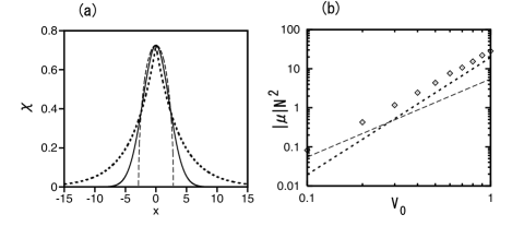
Figure 2: (a) The numerically found profile of stationary wave functions $\chi_{1}(r)=\chi_{2}(r)$ at $V_{0}=1$ and $\gamma=0.9$, with $N_{1}=N_{2}=4\pi$, and its comparison with the exponential analytical approximation given by Eq. (17) and the TF approximation Eq. (20) (the short- and long-dashed lines, respectively). (b) The chain of rhombuses depicts the numerically found relation between $|\mu|N^{2}$ and $V_{0}$ at $\gamma=0.9$. The short- and long-dashed lines represent the approximations provided by Eqs. (18) and (21), respectively.

The simplest global analytical approximation for the wave function of the GS was proposed in Ref. we1 as an interpolation between the asymptotic expansions (7), ignoring the corrections $\sim r^{s/2}$ and $r^{2}$, and the leading term in expansion (16):

$$\chi_{n}(r)\approx\chi_{\mathrm{misc}}^{(0)}e^{-\sqrt{-2\mu_{n}}r}.$$ (17)

The substitution of this interpolation into Eqs. (5) and (6), along with expression (9), yields an approximate relations between the chemical potentials and squared average radius of two components, and their norms:

$$\mu_{n} = -2\left[\frac{\pi V_{0}}{(1+\gamma)N_{n}}\right]^{2},$$ (18)

$$\left\langle r_{n}^{2}\right\rangle = \left[\frac{(1+\gamma)N_{n}}{2\pi V_{0}}\right]^{2}.$$ (19)

Comparison of Eq. (18) with numerical results is shown in Fig. 2(b) by the dashed line. This approximation is accurate for sufficiently small $V_{0}$, but becomes inaccurate for large $V_{0}$.

For large $V_{0}$, the Thomas-Fermi (TF) approximation can be applied to the balanced mixture, with $N_{1}=N_{2}\equiv N$. In this approximation, the derivative terms are neglected in Eq. (LABEL:stat), which yields (for $\chi_{1}=\chi_{2}\equiv\chi$)

$$\chi_{\mathrm{TF}}(r)=\left\{\begin{array}[]{c}\sqrt{\left(V_{0}+\mu r^{2}\right)/\left(1+\gamma\right)}\,,~{}~{}\mathrm{at}~{}~{}r<R_{0}\equiv\sqrt{V_{0}/(-\mu)},\\ 0,~{}~{}\mathrm{at}~{}~{}r>R_{0}~{}.\end{array}\right.$$ (20)

The substitution of approximation (20) into Eqs. (5) and (6) yields the corresponding $\mu_{\mathrm{TF}}(N)$ and $\left\langle r_{\mathrm{TF}}^{2}\right\rangle(N)$ relations,

$$\mu_{\mathrm{TF}} = -\frac{64\pi^{2}V_{0}^{3}}{9(1+\gamma)^{2}N^{2}},$$ (21)

$$\left\langle r_{\mathrm{TF}}^{2}\right\rangle = \frac{5}{\pi^{3}}\left[\frac{3\left(1+\gamma\right)N}{16V_{0}}\right]^{2}\equiv\frac{5}{4\pi}R_{0}^{2},$$ (22)

where $N$ is the norm of one component [recall $R_{0}$ is the TF cutoff radius defined in Eq. (20); naturally, the average radius is smaller than the cutoff value]. Analytical approximations (17) and (20) (shown by the short- and long-dashed lines, respectively) are compared with the numerically found profile of the GS in Fig. 2(b), demonstrating that the TF approximation provides for a good description of the core part of the GS.

An obvious corollary of Eqs. (LABEL:stat) and (5) are exact scaling relations between $\mu$, $\left\langle r^{2}\right\rangle$ and $N$:

$$\mu \propto -1/N^{2},$$ (23)

$$\left\langle r^{2}\right\rangle \propto N^{2},$$ (24)

for fixed $V_{0}$ and $\gamma$, cf. particular examples given by Eqs. Note that scaling (23) meets the “anti-Vakhitov-Kolokolov” criterion, which plays the role of the condition necessary for the stability of localized modes supported by repulsive nonlinearities we3 . Thus, product $|\mu|N^{2}$ does not depend on $N$, but does depend on the pull-to-the-center constant, $V_{0}$. This numerically found dependence is shown by a chain of rhombuses in Fig. 1(b) on the double-logarithmic scale. It is seen that $|\mu|N^{2}$ increases with $V_{0}$ monotonously. In the same plot, the short- and long-dashed lines show analytical approximations for the same dependence given by Eq. (18) and (21), respectively. It can be concluded that, quite naturally, the TF approximation works better for larger $V_{0}$, while the interpolation (17) is more accurate for smaller $V_{0}$.

Examples of numerically generated profiles of imbalanced miscible GSs is shown in Fig. 3(a) at $V_{0}=2$ and $\gamma=0.9$ for $N_{1}=4\pi$ and $N_{2}=2\pi$. Imbalanced miscible states with $\mu_{1}\neq\mu_{2}$ and $N_{1}\neq N_{2}$ are still characterized by equal values of $\chi_{1,2}(r=0)$, in agreement with Eq. (9), but different constants $d_{1,2}^{(1)}$ in expansion (7), see Eq. (12).

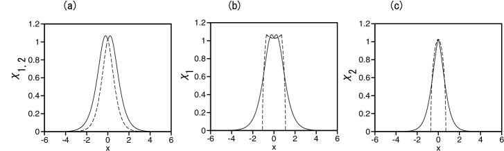
Figure 3: (a) $\chi_{1}$ (continuous) and $\chi_{2}$ (dashed) components of the imbalanced miscible ground state at $V_{0}=2$ and $\gamma=0.9$, with $N_{1}=4\pi$ and $N_{2}=2\pi$. (b) and (c): Comparison of the numerical result (continuous lines) with the two-layer TF approximation (dashed lines) for $\chi_{1}(r)$ and $\chi_{2}(r)$.

In the case of the strong pull to the center, $V_{0}\gg 1$, the TF approximation, which has yielded Eqs. (20) and (21) for the balanced miscible GS, neglecting the derivatives in Eq. (LABEL:stat), can be generalizes for imbalanced states, with $\mu_{1}\neq\mu_{2}$. For the sake of the definiteness, we set $\mu_{2}\leq\mu_{1}$ (i.e., $\left|\mu_{1}\right|\leq\left|\mu_{2}\right|$, as the chemical potentials of the bound states are negative).

The TF approximation for imbalanced configuration is constructed in a two-layer form, technically similar to that applied to the so-called symbiotic gap solitons in Ref. Thawatchai . In the inner layer,

$$r^{2}<r_{0}^{2}\equiv\frac{1-\gamma}{\gamma\mu_{1}-\mu_{2}}V_{0},$$ (25)

both wave functions are different from zero:

$$\chi_{n}^{\mathrm{(inner)}}(r)=\sqrt{\frac{V_{0}}{1+\gamma}-\frac{\gamma\mu_{3-n}-\mu_{n}}{1-\gamma^{2}}r^{2}}.$$ (26)

In the outer layer, only one component is present, in the framework of the TF approximation: $\chi_{2}\equiv 0$,

$$\chi_{1}^{\mathrm{(outer)}}(r)=\left\{\begin{array}[]{c}\sqrt{V_{0}+\mu_{1}r^{2}},~{}\mathrm{at}~{}~{}r_{0}^{2}\leq r^{2}\leq R_{0}^{2}\equiv-V_{0}/\mu_{1},\\ 0,~{}\mathrm{at}~{}~{}r^{2}\geq R_{0}^{2}~{}.\end{array}\right.$$ (27)

Note that both components of the TF solution, given by Eqs. (25)-(27), are continuous at $r=r_{0}$ and $r=R_{0}$. It is also worthy to note that $\chi_{1}^{\mathrm{(inner)}}(r)$ is a decreasing or increasing function of $r$ in the cases of $\left|\mu_{1}\right|<\left|\mu_{2}\right|<|\mu_{1}|/\gamma$ and $\left|\mu_{2}\right|>|\mu_{1}|/\gamma$, respectively. The two-layer TF approximation for a typical imbalanced GS is compared to its numerical counterpart in Figs. 3(b,c).

The corresponding approximation for the dependence between the chemical potentials and norms of the second component is produced by the straightforward integration of expression (26), cf. Eq. (5):

$$N_{2}^{\mathrm{(TF)}}(\mu_{1},\mu_{2})=4\pi\int_{0}^{r_{0}}\left[\chi_{2}^{\mathrm{(inner)}}(r)\right]^{2}dr=\frac{8\pi}{3}\frac{\sqrt{1-\gamma}}{1+\gamma}V_{0}^{3/2}\left(\gamma\mu_{1}-\mu_{2}\right)^{-1/2}.$$ (28)

The corresponding expression for the norm of the first component is very cumbersome, therefore we give it here only for the limit case of $N_{1}\gg N_{2}$, i.e., $\left|\mu_{2}\right|\gg\left|\mu_{1}\right|$:

$$N_{1}^{\mathrm{(TF)}}\approx\frac{8\pi}{3}V_{0}^{3/2}\left(-\mu_{1}\right)^{-1/2}.$$ (29)

Note that dependences (28) and (29) obey the generic scaling law (23). Expressions for the TF radii of the two imbalanced components can be derived too, cf. Eq. (22), but they are very cumbersome.

III.2 Immiscible ground states

As said above, in the case of $\gamma>1$ relevant states are immiscible ones, which are approximated, at small $r$, by Eqs. (7), (11), (12), and (13) for $\chi_{1}(r)$, with $\mu_{2}$ substituted by $\mu_{1}$ in the two latter equations, and by Eq. (15) for $\chi_{2}(r)$. A generic example of the immiscible GS found at $V_{0}=1,\gamma=1.2$ and $N_{1}=N_{2}=0.8\pi$ is displayed in Fig. 4(a), and Fig. 4(b) shows the double-logarithmic plot of $\chi_{2}(r)$ at $V_{0}=1$, comparing it to the analytical prediction given by Eq. (15). Further, Fig. 4(c) displays relations between chemical potentials and norms of both components of the immiscible GSs. The dashed curves in the latter figure verify the validity of scaling relation (23) in the present case.

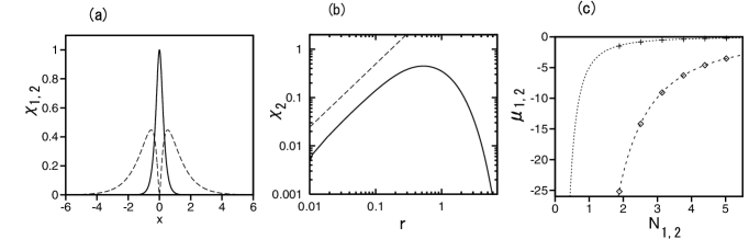
Figure 4: (a) An example of numerically found profiles $\chi_{1}(r)$ and $\chi_{2}(r)$ (the solid and dashed lines) of the immiscible ground state for $V_{0}=1,\gamma=1.2$ and equal norms of the two components, $N_{1}=N_{2}=0.8\pi$, while $\mu_{1}=-14.2$ and $\mu_{2}=-0.84$. (b) The double-logarithmic plot of the same component $\chi_{2}(r)$. The dashed straight line shows, for the sake of the comparison, the analytical prediction provided by Eq. (15). (c) Chains of symbols depict relations $\mu_{1,2}(N_{1,2})$ for the immiscible ground states at $V_{0}=1,\gamma=1.2$. Dashed lines are empiric fits to scaling (23), $\mu_{1}=-89/N^{2}$ and $\mu_{2}=-5/N^{2}$.

The TF approximation produces a two-layer solution for the immiscible state. In the inner layer,

$$r^{2}<r_{0}^{2}=\frac{(\gamma-1)V_{0}}{\gamma\mu_{1}-\mu_{2}},$$

the approximation yields

$$\chi_{1}(r)=\sqrt{V_{0}+\mu_{1}r^{2}},\;\chi_{2}(r)=0.$$ (30)

In the outer layer, with $r_{0}^{2}<r^{2}<R_{0}^{2}=V_{0}/(-\mu_{2})$, the result is

$$\chi_{1}(r)=0,\;\chi_{2}(r)=\sqrt{V_{0}+\mu_{2}r^{2}}.$$ (31)

In these solutions, $\mu_{1}$ and $\mu_{2}$ are related to the norms.

$$N_{1}^{(\mathrm{TF})}(\mu_{1},\mu_{2})=4\pi\int_{0}^{r_{0}}\chi_{1}(r)^{2}dr=4\pi r_{0}\frac{\mu_{2}-(2/3)\gamma\mu_{1}-\mu_{1}/3}{\mu_{2}-\gamma\mu_{1}},$$

$$N_{2}^{(\mathrm{TF})}(\mu_{1},\mu_{2})=4\pi\int_{r_{0}}^{R_{0}}\chi_{2}^{2}(r)dr$$

$$=4\pi\left[\frac{2}{3}\frac{V_{0}^{3/2}}{\sqrt{-\mu_{2}}}-\sqrt{\gamma-1}\left(\frac{V_{0}}{(\mu_{2}-\gamma\mu_{1}}\right)^{3/2}\left(\frac{2}{3}\mu_{2}+\frac{1}{3}\gamma\mu_{2}-\gamma\mu_{1}\right)\right].$$

Figure 5 compares this TF approximation with numerical results.

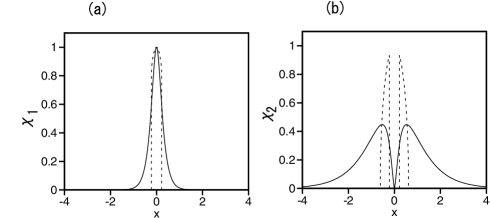
Figure 5: (a) and (b): The comparison of the numerically found profiles for components $\chi_{1}(r)$ and $\chi_{2}(r)$ of the immiscible ground state, shown in Fig. 4(a) (solid lines), with the respective TF approximations, given by Eqs. (30) and (31), respectively (continuous lines).

III.3 Characterization of the weak phase transition

Finally, it is relevant to discuss how the weak phase transition, predicted above at $V_{0}=\widetilde{V}_{0}^{(\mathrm{cr})}\equiv 1/2$, may manifest itself in terms of experimentally measurable quantities. To this end, it is relevant to consider dependences of the GS’s characteristics on $V_{0}$ at a fixed value of the norm, $N$, which is sufficient to do for the single-component model (this problem was not considered previously in Ref. we2 ). In fact, scaling relations (23) and (24) demonstrate that these dependences have the same form at all constant values of $N$.

In the experiment, the variation of $V_{0}$ may be possible in the gas composed of excited atoms: because the dipole moment of the atom in the Rydberg state scales with the principal quantum number, $n$, as $n^{2}$, the change $n\rightarrow n+1$ will give rise, according to Eq. (1), to a relative variation of the attraction constant, $\left|\Delta V_{0}\right|/V_{0}\approx 2/n$, which is small for sufficiently large $n$.

First, Fig. 6(a) shows that the dependence of the chemical potential on $V_{0}$ does not show any visible peculiarity at $V_{0}=1/2$ (however, the chemical potential is not an observable quantity). On the other hand, the plot for $\left\langle r^{2}\right\rangle$ versus $V_{0}$, displayed in Fig. 6(b), shows a subtle but observable feature: the change of the slope of the dependence from $-85$ to $-54$ (in the scaled units adopted in this work) in a small vicinity of the the phase-transition point, as illustrated by means of the two tangent lines. Thus, the experimental observation of the size of the ground state may reveal the occurrence of the phase transition.

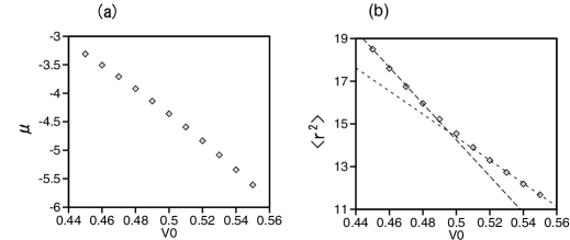
Figure 6: (a) The dependence of the chemical potential on the attraction strength, $V_{0}$, for a fixed norm, $N=4\pi$, in the miscible state at $\gamma=0.9$. (b) The dependence of the average squared radius of the ground state, calculated as per Eq. (6), on $V_{0}$, in the same case. Straight tangent lines illustrate the change in the slope of the dependence around the weak-phase-transition point, $V_{0}=1/2$.

IV The binary system with the single component pulled to the center

Next, we consider the binary system with the attractive potential $-V_{0}/r^{2}$ acting only on the first species. In this case, we adopt the combination of the intra-species self-repulsion and attraction between the species, i.e., $\gamma<0$ in the accordingly modified system of Eqs. (LABEL:GP) and (LABEL:stat):

$$i\frac{\partial\phi_{1}}{\partial t} = -\frac{1}{2}\nabla^{2}\phi_{1}+(|\phi|^{2}+\gamma|\phi_{2}|^{2})\phi_{1}-\frac{V_{0}}{r^{2}}\phi_{1},$$

$$i\frac{\partial\phi_{2}}{\partial t} = -\frac{1}{2}\nabla^{2}\phi_{2}+(\gamma|\phi_{1}|^{2}+|\phi_{2}|^{2})\phi_{2},$$

$$\mu_{1}\chi_{1} = -\frac{1}{2}\chi_{1}^{\prime\prime}-\frac{V_{0}}{r^{2}}\chi_{1}+(\chi_{1}^{2}+\gamma\chi_{2}^{2})\frac{\chi_{1}}{r^{2}},$$

$$\mu_{2}\chi_{2} = -\frac{1}{2}\chi_{2}^{\prime\prime}+(\chi_{2}^{2}+\gamma\chi_{1}^{2})\frac{\chi_{2}}{r^{2}}.$$

Solutions to Eqs. (LABEL:stat1) can be again sought for in the form of expansion (7) at $r\rightarrow 0$, which yields, instead of Eqs. (LABEL:chichi), a system of algebraic relations

$$\chi_{1}^{(0)}\left[\left(\chi_{1}^{(0)}\right)^{2}+\gamma\left(\chi_{2}^{(0)}\right)^{2}\right] = V_{0}\chi_{1}^{(0)},$$

$$\chi_{2}^{(0)}\left[\left(\chi_{2}^{(0)}\right)^{2}+\gamma\left(\chi_{1}^{(0)}\right)^{2}\right] = 0.$$

It is easy to see that, in the present case with $\gamma<0$, a nontrivial solution to Eqs. (LABEL:chichi1) exists for $|\gamma|~{}<1$:

$$\chi_{1}^{(0)}=\sqrt{V_{0}/(1-\gamma^{2})},~{}\chi_{2}^{(0)}=\sqrt{-\gamma}\chi_{10}.$$ (35)

Further, the interpolation ansatz, following the pattern of Eq. (17),

$$\chi_{n}(x)=\chi_{n}^{(0)}\exp\left(-\sqrt{-2\mu_{n}}r\right),$$ (36)

with $\chi_{n}^{(0)}$ given by Eq. (35), predicts the following relations between the chemical potentials and norms of the two components:

$$\mu_{1}=-\frac{1}{2}\left(\frac{2\pi V_{0}N_{1}}{1-\gamma^{2}}\right)^{2},\ \mu_{2}=-\frac{1}{2}\left(\frac{2\pi\gamma V_{0}N_{2}}{1-\gamma^{2}}\right)^{2}.$$ (37)

Figure 7(a) displays a typical example of the numerically found profiles of $\chi_{1}(r)$ and $\chi_{2}(r)$, for $V_{0}=1,\gamma=-0.7,N=4\pi$. Further, Figs. 7(b) and (c) compare the numerical profiles of $\chi_{1}(r)$ and $\chi_{2}(r)$ with the analytical approximations based on ansätze (20), (35) and (36).

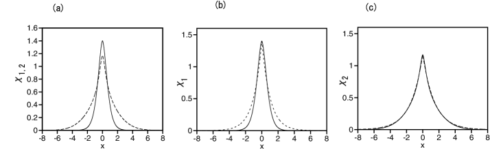
Figure 7: (a) Numerically found profiles of stationary wave functions $\chi_{1}(r)$ and $\chi_{2}(r)$ (the taller and lower ones, respectively) in the model based on Eqs. (LABEL:GP1) and (LABEL:stat1), for $V_{0}=1,\gamma=-0.7$. $\mu_{1}=-2.59$ and $\mu_{2}=-0.18$. (b) and (c): The comparison of $\chi_{1}(r)$ and $\chi_{2}(r)$ with the analytical approximations provided by Eq. (36).

The family of the GSs in the present version of the binary system is characterized by dependences of the chemical potentials of the two components on coupling constant $\gamma$, see Fig. 8(a), and on $N_{1}=N_{2}\equiv N$ in Fig. 8(b). In both panels, the dashed and dotted lines depict the analytical prediction for $\mu_{1}$ and $\mu_{2}$ produced by Eq. (37). Thus, it is concluded that the analytical approximation provide for quite an accurate description of the $\chi_{2}$ component (the one which is not pulled to the center), while the approximation for $\chi_{1}$ is less accurate.

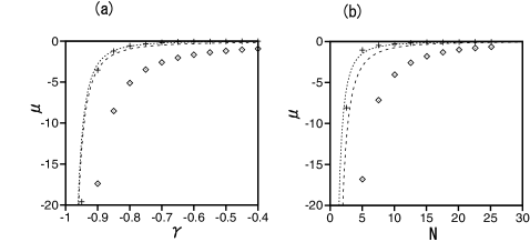
Figure 8: (a) The chemical potentials of the two components, $\mu_{1}$ ($\Diamond$) and $\mu_{2}$ ($+$), in the model based on Eqs. (LABEL:GP1) and (LABEL:stat1), versus $\gamma$ for $N_{1}=N_{2}=4\pi$ and $V_{0}=1$. (b) The same chemical potentials versus $N_{1}=N_{2}\equiv N$ for $\gamma=-0.7$ and $V_{0}=1$. The dashed and dotted curves show the analytical prediction (37).

Finally, the two-layer TF approximation can be applied to the present system too, under conditions $\gamma^{2}<1$ and $\mu_{2}<\mu_{1}<0$. In particular, the solution in the inner layer,

$$r^{2}\leq r_{0}^{2}\equiv-\frac{|\gamma|}{\mu_{2}+|\gamma|\mu_{1}}V_{0},$$

cf. Eq. (25), takes the following form, cf. Eq. (26):

$$\chi_{1}^{\mathrm{(inner)}}(r) = \sqrt{\frac{V_{0}+\left(\mu_{1}+|\gamma|\mu_{2}\right)r^{2}}{1-\gamma^{2}}},$$

$$\chi_{2}^{\mathrm{(inner)}}(r) = \sqrt{\frac{|\gamma|V_{0}+\left(\mu_{2}+|\gamma|\mu_{1}\right)r^{2}}{1-\gamma^{2}}},$$

the corresponding dependence of the norm on the chemical potentials being

$$N_{2}^{\mathrm{(TF)}}(\mu_{1},\mu_{2})=\frac{8\pi}{3}\left(|\gamma|V_{0}\right)^{2/3}\left[-\left(\mu_{2}+|\gamma|\mu_{1}\right)\right]^{-1/2},$$

cf. Eq. (28). In the outer layer, the TF solution takes the same from as in Eq. (27).

V Conclusion

The aim of this work is to extend the recent analysis of the suppression of the quantum collapse, induced by action of the attractive potential $-V_{0}r^{-2}$ in the 3D space, by the repulsive nonlinearity in the bosonic gas, to the binary miscible and immiscible gases. We have concluded that the GS (ground state) which the respective linear Schrödinger equation fails to create, emerges in the nonlinear system. The GSs were found in the numerical form, and approximated by means of several analytical methods, such as the TF (Thomas-Fermi) approximation, which is relevant for large $V_{0}$. An essential finding is that both balanced and imbalanced miscible gases feature the weak phase transition in the GS, in the form of the analyticity-breaking change in the structure of the wave functions at small $r$. The binary system with the attraction between the species (rather than repulsion) has been considered too, in the case when the attractive central potential acts on a single component.

References

- (1) L. D. Landau and E. M. Lifshitz, Quantum Mechanics: Nonrelativistic Theory (Nauka, Moscow, 1974).
- (2) K. S. Gupta and S. G. Rajeev, Phys. Rev. D 48, 5940 (1993); H. E. Camblong, L. N. Epele, H. Fanchiotti, and C. A. García Canal, Phys. Rev. Lett. 85, 1590 (2000); Ann. Phys. (N.Y.) 287, 57 (2001).
- (3) H. Sakaguchi and B. A. Malomed, Phys. Rev. A 83, 013907 (2011).
- (4) L. Pitaevskii and S. Stringari, Bose-Einstein Condensation (Clarendon Press: Oxford, 2003).
- (5) J. Deiglmayr, A. Grochola, M. Repp, K. Mörtlbauer, C. Glück, J. Lange, O. Dulieu, R. Wester, and M. Weidemüller, Phys. Rev. Lett. 101, 133004 (2008).
- (6) S. Ospelkaus, K.-K. Ni, G. Quéméner, B. Neyenhuis, D. Wang, M. H. G. de Miranda, J. L. Bohn, J. Ye, and D. S. Jin, Phys. Rev. Lett. 104, 030402 (2010).
- (7) S. Schmid, A. Härter, and J. H. Denschlag, Phys. Rev. Lett. 105, 133202 (2010).
- (8) I. Mourachko, D. Comparat, F. de Tomasi, A. Fioretti, P. Nosbaum, V. M. Akulin, and P. Pillet, Phys. Rev. Lett. 80, 253 (1998); W. R. Anderson, J. R. Veale, and T. F. Gallagher, ibid. 80, 249 (1998); M. D. Lukin, M. Fleischhauer, and R. Côté, ibid. 87, 037901 (2001); D. Tong, S. M. Farooqi, J. Stanojevic, S. Krishnan, Y. P. Zhang, R. Côté, E. E. Eyler, and P. L. Gould ibid. 93, 063001 (2004); M. Mayle, B. Hezel, I. Lesanovsky, and P. Schmelcher, ibid. 99, 113004 (2007).
- (9) T. F. Gallagher and P. Pillet, Adv. At. Mol. Opt. Phys. 56, 161 (2008).
- (10) J. E. Johnson and S. L. Rolston, Phys. Rev. A 82, 033412 (2010).
- (11) H. Sakaguchi and B. A. Malomed, Phys. Rev. A 84, 033616 (2011).
- (12) J. Denschlag and J. Schmiedmayer, Europhys. Lett. 38, 405 (1997).
- (13) J. Denschlag, G. Umshaus, and J. Schmiedmayer, Phys. Rev. Lett. 81, 737 (1998).
- (14) A. Muñoz Mateo and V. Delgado, Phys. Rev. A 77, 013617 (2008).
- (15) M. Zaccanti, C. D’Errico, F. Ferlaino, G. Roati, M. Inguscio, and G. Modugno, Phys. Rev. A 74, 041605(R) (2006); G. Thalhammer, G. Barontini, L. De Sarlo, J. Catani, F. Minardi, and M. Inguscio, Phys. Rev. Lett. 100,210402 (2008); S. B. Papp, J. M. Pino, and C. E. Wieman, ibid. 101, 040402 (2008); K. Enomoto, K. Kasa, M. Kitagawa, and Y. Takahashi, ibid. 101, 203201 (2008); S. Tojo, Y. Taguchi, Y. Masuyama, T. Hayashi, H. Saito, and T. Hirano, Phys. Rev. A 82,033609 (2010).
- (16) I. Bloch, J. Dalibard, and W. Zwerger, Rev. Mod. Phys. 80, 885 (2008).
- (17) V. P. Mineev, Zh. Eksp. Teor. Fiz. 67, 263 (1974) [Sov. Phys.—JETP 40, 132 (1974)].
- (18) C. J. Myatt E. A. Burt, R. W. Ghrist, E. A. Cornell, and C. E. Wieman, Phys. Rev. Lett. 78 586 (1997); H. Pu and N. P. Bigelow, ibid. 80 1130 (1998); D. S. Hall, M. R. Matthews, J. R. Ensher, C. E. Wieman, and E. A. Cornell, ibid. 81, 1539 (1998); J. O. Indekeu and B. Van Schaeybroeck, ibid. 93, 210402 (2004); J. Sabbatini, W. H. Zurek, and M. J. Davis, ibid. 107, 230402 (2011); D. J. McCarron, H. W. Cho, D. L. Jenkin, M. P. Köppinger, and S. L. Cornish, Phys. Rev. A 84, 011603(R) (2011); M. A. Hoefer, J. J. Chang, C. Hamner, and P. Engels, ibid. 84, 041605(R) (2011); F. Tsitoura, V. Achilleos, B. A. Malomed, D. Yan, P. G. Kevrekidis, and D. J. Frantzeskakis, ibid. 87, 063624 (2013).
- (19) I. M. Merhasin, B. A. Malomed and R. Driben, J. Phys. B: At. Mol. Opt. Phys. 38, 877 (2005).
- (20) Y. V. Kartashov, V. A. Vysloukh, L. Torner, and B. A. Malomed, Opt. Lett. 36, 4587 (2011); L. Wen, W. M. Liu, Y. Cai, J. M. Zhang, and J. Hu, Phys. Rev. A 85, 043602 (2012).
- (21) B. Deconinck, PO. G. Kevrekidis, H. E. Nistazakis, and D. J. Frantzeskakis, Phys. Rev. A 70, 063605 (2004); S. K. Adhikari and B. A. Malomed, ibid. 79, 015602 (2009); N. Dror, B. A. Malomed, and J. Zeng, Phys. Rev. E 84, 046602 (2011).
- (22) C. J. Wang, C. Gao, C. M. Jian, and H. Zhai, Phys. Rev. Lett. 105, 160403 (2010); H. Sakaguchi and B. Li, Phys. Rev. A 87, 015602 (2013); D. A. Zezyulin, R. Driben, V. V. Konotop, and B. A. Malomed, Phys. Rev. A, in press.
- (23) M. Trippenbach, K. Goral, K. Rzazewski, B. Malomed, and Y. B. Band, J. Phys. B: At. Mol. Opt. 33, 4017 (2000); P. Ohberg and L. Santos, Phys. Rev. Lett. 86, 2918 (2001); S. Coen and M. Haelterman, ibid. 87, 140401 (2001); D. T. Son and M. A. Stephanov, Phys. Rev. 65, 063621 (2002); R. A. Barankov, ibid. 66, 013612 (2002); B. A. Malomed, H. E. Nistazakis, D. J. Frantzeskakis, and P. G. Kevrekidis, ibid. 70, 043616 (2004); P. G. Kevrekidis, H. E. Nistazakis, D. J. Frantzeskakis, B. A. Malomed, and R. Carretero-González, Eur. Phys. J. D 28, 181 (2004); H. Saito, Y. Kawaguchi, and M. Ueda, Phys. Rev. A 75, 013621 (2007); H. E. Nistazakis, D. J. Frantzeskakis, P. G. Kevrekidis, B. A. Malomed, R. Carretero-González, and A. R. Bishop, ibid. 76, 063603 (2007); B. Van Schaeybroeck, ibid. 78, 023624 (2008); Z. D. Li, Q.-Y. Li, P. B. He, J. Q. Liang, W. M. Liu, and G. S. Fu, ibid. 81, 015602 (2010).
- (24) V. S. Shchesnovich, A. M. Kamchatnov, and R. A. Kraenkel, Phys. Rev. A 69, 033601(2004); J. Wei and T. Weth, Arch. Rat. Mech. Anal. 190, 83 (2008); J. Jin, S. Zhang, and W. Han, J. Phys. B: At. Mol. Opt. Phys. 44, 165302 (2011); R. W. Pattinson, T. P. Billam, S. A. Gardiner, D. J. McCarron, H. W. Cho, S. L. Cornish, N. G. Parker, and N. P. Proukakis, Phys. Rev. A 87, 013625 (2013).
- (25) H. Sakaguchi and B. A. Malomed, Phys. Rev. A 81, 013624 (2010).
- (26) A. Roeksabutr, T. Mayteevarunyoo, and B. A. Malomed, Opt. Exp. 20, 24559 (2012).
- (27) G. E. Astrakharchik, D. M. Gangardt, Y. E. Lozovik, and I. A. Sorokin, Phys. Rev. E 74, 021105 (2006).
- (28) A. V. Chubukov, C. Pepin, and J. Rech, Phys. Rev. Lett. 92, 147003 (2004); T. R. de Oliveira, G. Rigolin, M. C. de Oliveira, and E. Miranda, ibid. 97, 170401 (2006); Y. Yamaji, T. Misawa, and M. Imada, J. Phys. Soc. Jpn. 75, 094719 (2006); F. Mazzanti,G. E. Astrakharchik, J. Boronat, and J. Casulleras, Phys. Rev. A 77, 043632 (2008); J.-H. Zhao and H.-Q. Zhou, Phys. Rev. B 80, 014403 (2009); B. Q. Liu, B. Shao, J. G. Li, J. Zou, and L. A. Wu, Phys. Rev. A 83, 052112 (2011); Y. Yao, H.-W. Li, C. M. Zhang, Z. Q. Yin, W. Chen, G. C. Guo, and Z. F. Han, ibid. 86, 042102 (2012).
- (29) J. Wang, C. A. Cerdeirina, M. A. Anisimov, and J. V. Sengers, Phys. Rev. E 77, 031127 (2008).