The influence of the magnetic field on the spectral properties of blazars

Abstract

We explore the signature imprinted by dynamically relevant magnetic fields on the spectral energy distribution (SED) of blazars. It is assumed that the emission from these sources originates from the collision of cold plasma shells, whose magnetohydrodynamic evolution we compute by numerically solving Riemann problems. We compute the SEDs including the most relevant radiative processes and scan a broad parameter space that encompasses a significant fraction of the commonly accepted values of not directly measurable physical properties. We reproduce the standard double hump SED found in blazar observations for unmagnetized shells, but show that the prototype double hump structure of blazars can also be reproduced if the dynamical source of the radiation field is very ultrarelativistic both, in a kinematically sense (namely, if it has Lorentz factors $\gtrsim 50$) and regarding its magnetization (e.g., with flow magnetizations $\sigma\simeq 0.1$). A fair fraction of the blazar sequence could be explained as a consequence of shell magnetization: negligible magnetization in FSRQs, and moderate or large (and uniform) magnetization in BL Lacs. The predicted photon spectral indices ($\Gamma_{\rm ph}$) in the $\gamma-$ray band are above the observed values ($\Gamma_{\rm ph,obs}\lesssim 2.6$ for sources with redshifts $0.4\leq z\leq 0.6$) if the magnetization of the sources is moderate ($\sigma\simeq 10^{-2}$).

1 Introduction

Blazars are a type of radio-loud active galactic nuclei (AGN) whose jets are pointing very close to the line of sight towards the observer (e.g., Urry & Padovani, 1995). They can be subdivided in two main groups: BL Lac objects, whose spectrum is featureless or shows only weak absorption lines and flat-spectrum radio quasars (FSRQs), which show broad emission lines in the optical spectrum (e.g., Giommi et al., 2012). Blazars are commonly classified according to the relative strength of their observed spectral components. Those spectral components are associated to the contribution of a relativistic jet (non-thermal emission), the accretion disk and the broad-line region (thermal radiation), and the light from the host, usually a giant elliptical galaxy. The broadest component of the spectrum is the non-thermal one, and it spans the whole electromagnetic frequency range, usually displaying two broad peaks. The lower-frequency part is due to the synchrotron emission (it usually peaks in the range $10^{12}$-$10^{17}$ Hz), while the high-frequency region is believed to be due to the inverse-Compton scattering (e.g., Fossati et al., 1998).

In this work we concentrate exclusively on the contribution from the relativistic jet. The internal shock (IS) scenario (e.g., Rees & Meszaros, 1994; Spada et al., 2001; Mimica et al., 2004) has been successful in explaining many of the features of the blazar variability. At the core of the IS scenario is the idea that the presence of relative motions in the relativistic jet will produce ‘collisions’ of cold and dense blobs of plasma (shells). In the course of the shell collision the plasma is shocked and part of the jet kinetic energy is dissipated at relatively weak internal shocks, which shall account for the observed flares in the light curves of these events. In the past two decades this scenario has been thoroughly explored using analytic and (simplified) numerical modeling (Kobayashi et al., 1997; Daigne & Mochkovitch, 1998; Spada et al., 2001; Bošnjak et al., 2009; Daigne et al., 2011) and by means of numerical hydrodynamics simulations (Kino et al., 2004; Mimica et al., 2004, 2005, 2007).

More recently, the effects of strong magnetic fields on the shell collisions have been investigated. The shocked plasma is believed to be magnetized, to some extent, since we observe radiation that can be best fit as synchrotron emission of particles accelerated in internal plasma collisions. However, we do not really know the degree of magnetization of the jet flow, and whether its magnetic energy is being dissipated in addition to its kinetic energy. In the case of moderate or strong magnetic fields the IS scenario has to be modified to account for the differences in dynamics (e.g., the suppression of one of the two shocks resulting in a binary collision Fan et al., 2004; Mimica & Aloy, 2010) and the emission properties of the flares (Mimica et al., 2007; Mimica & Aloy, 2012).

This work continues along the lines sketched in our previous paper (Mimica & Aloy, 2012, MA12 in the rest of the text). MA12 extends the work on the dissipation (dynamic efficiency) of magnetized IS (Mimica & Aloy, 2010) by including radiative processes in a manner similar to that of the recent detailed models for the computation of the IS emission (Böttcher & Dermer, 2010; Joshi & Böttcher, 2011; Chen et al., 2011). In MA12 we assume a constant flow luminosity, but vary the degree of the shell magnetization in order to investigate the consequences of that variation for the observed spectra and light curves. The radiative efficiency of a single shell collision is found to be largest when one of the colliding shells is very magnetized, while the other one has weak or no magnetic field. We proposed a way to distinguish observationally between weakly and strongly magnetized shell collisions through the comparison of the inverse-Compton and synchrotron maximum frequencies and fluences.

One of the limitations of MA12 is that only shell magnetization is varied (albeit with a relatively dense coverage of the potential parameter space), leaving the rest of the parameters unchanged. In this work we present results of a more systematic parametric study where we consider three combinations of the shell magnetizations, which MA12 found to be of interest, but vary both kinematical (shell Lorentz factors and relative velocity) and extrinsic parameters (jet viewing angle), while the microphysical parameters are fixed to typically accepted values.

In Section 2 we discuss the method and list the models considered in the present work. Section 3 presents the results which are discussed and summarized in Section 4.

2 Modeling dynamics and emission from internal shocks

In this section we summarize the method of MA12, which is used to model the dynamics of shell collisions and the resulting non-thermal emission (we follow Sections 2, 3 and 4 of MA12). We also discuss the three families of numerical models used in this work.

2.1 Dynamics of shell collisions

Assuming a cylindrical outflow and neglecting the jet lateral expansion (e.g., Mimica et al., 2004) we can simplify the problem of colliding shells to a one-dimensional interaction of two cylindrical shells with cross-sectional radius $R$ and thickness $\Delta r$. We fix the luminosity $L$ of the outflow to a constant value and allow the shell Lorentz factor $\Gamma$ and the magnetization $\sigma$ (see Eq. 2 in Appendix A for definition) to vary. This allows us to compute the number density in an unshocked shell (see Eq. 3 of MA12):

$$n=\displaystyle{\frac{L}{\pi R^{2}m_{p}c^{3}\left[\Gamma^{2}(1+\epsilon+\chi+\sigma)-\Gamma\right]\sqrt{1-\Gamma^{-2}}}}\ ,$$ (1)

where $m_{p}$ and $c$ are the proton mass and the speed of light, $\chi:=P/\rho c^{2}\ll 1$ is the ratio between the thermal pressure $P$ and the rest-mass energy density, and $\epsilon$ is the specific internal energy (see Eq. 2 of MA12).

Once the number density, the thermal pressure, the magnetization, and the Lorentz factor of the faster (left) and the slower (right) shell have been determined, we use the exact Riemann solver of Romero et al. (2005) to compute the evolution of the shell collision. In particular, we compute the properties of the shocked shell fluid (shock velocity, compression factor, magnetic field) which we then use to obtain the synthetic observational signature (see the following section).

2.2 Non-thermal particles and emission

For the readers benefit, we briefly summarize Sections 3.1 and 3.2 of MA12 on the assumptions about the distribution of the dissipated unshocked shell kinetic energy among the electrons and the magnetic fields.

We assume that a stochastic magnetic field $B_{S,st}$ is created at shocks. The strength of this field is parametrized by assuming that the magnetic field energy density is a fraction $\epsilon_{B}$ of the dissipated kinetic energy, i.e. $B_{S,st}=\sqrt{8\pi\epsilon_{B}u_{S}}$, where $u_{S}$ is the internal energy density in the shocked shell, obtained by the exact Riemann solver. Since we study the evolution of plasma shells with arbitrary degrees of magnetization carried out by macroscopic fields $B_{S,mac}$, the total magnetic field in the shell is defined as $B_{S}:=\sqrt{B_{S,mac}^{2}+B_{S,st}^{2}}$. $B_{S}$ is the field in which electrons are assumed to gyrate and emit synchrotron radiation. In practice, this means that the value of $\epsilon_{B}$ is irrelevant for models in which the macroscopic magnetization is large, since in such a case, $B_{S}\simeq B_{S,mac}$. The parameter $\epsilon_{B}$ only shapes the spectral properties of weakly magnetized models. In such models an increase in $\epsilon_{B}$ may modify (though not significantly) the spectral shape (e.g., Böttcher & Dermer, 2010, Fig. 9).

We assume that a fraction $\epsilon_{e}$ of the dissipated kinetic energy is used to accelerate electrons in the vicinity of shock fronts. We keep $\epsilon_{e}$ fixed in this work aiming to reduce the number of free parameters. We do not expect its possible variation to influence our results qualitatively (e.g., Böttcher & Dermer, 2010, show in Fig. 7 that a change in $\epsilon_{e}$ does not change the Compton dominance $A_{C}$).

In order to compute synthetic time-dependent multi-wavelength spectra and light curves, we assume that the dominant emission processes resulting from the shocked plasma are synchrotron, external inverse-Compton (EIC) and synchrotron self-Compton (SSC). The EIC component is the result of the up-scattering of near infrared photons (likely emitted from a dusty torus around the central engine of the blazar or from the broad line region) by the non-thermal electrons existing in the jet. We further consider that the observer’s line of sight makes an angle $\theta$ with the jet axis. A detailed description of how the integration of the radiative transfer equation along the line of sight is performed can be found in Section 4 of MA12.

2.3 Models

The main difference between this work and MA12 is that we allow for shell Lorentz factors and the viewing angle $\theta$ to vary. Table 3 shows the spectrum of model parameters that we consider in the next sections. In order to group our models according to the initial shell magnetizations we denote by letters W, M, S, S1 and S2 the following families of models:

• weakly magnetized, $\sigma_{L}=10^{-6},\sigma_{R}=10^{-6}$,

• moderately magnetized, $\sigma_{L}=10^{-2},\sigma_{R}=10^{-2}$,

• strongly magnetized, $\sigma_{L}=1,\sigma_{R}=10^{-1}$,

• strongly and equally magnetized, $\sigma_{L}=10^{-1},\sigma_{R}=10^{-1}$, and

• strongly magnetized, $\sigma_{L}=10^{-1},\sigma_{R}=1$.

The remaining three parameters, $\Gamma_{R}$, $\Delta g$ and $\theta$ can take any of the values shown in Table 3. We have considered three families of strongly magnetized models (S, S1 and S2), which differ in the distribution of the magnetization of the interacting shells. Our reference strongly magnetized model family is the S, since in MA12 we found that these models have the maximum dynamical efficiency. This set of models is supplemented with two additional families of models: S1, which accounts for shells having the same (high) magnetization, and S2, with parameters complementary of the S-family, and having the peculiarity that the colliding shells do not develop a forward shock (instead they form a forward rarefaction; see MA12) if $\Delta g\lesssim 1.5$, so that they only emit because of the presence of a reverse shock. For clarity, when we refer to a particular model we label it by appending values of each of these parameters to the model letter. For instance, S-G10-D1.0-T3 is the strongly magnetized model with $\Gamma_{R}=10$ (G10), $\Delta g=1.0$ (D1.0) and $\theta=3^{\circ}$ (T3). If we refer to a subset of models with one or two parameters fixed we use an abbreviated notation, where we skip any reference to the varying parameters in the family name. As an example of this abbreviated notation, in order to refer to all weakly magnetized models with $\Gamma_{R}=10$ and $\theta=5^{o}$ we use W-G10-T5, while all moderately magnetized models with $\Delta g=1.5$ are M-D1.5. We perform a systematic variation of parameters in order to find the dependence of the radiative signature on each of them separately, as well as their combinations by fixing, e.g. the Doppler factor ${\cal D}:=[\Gamma(1-\beta\cos{\theta})]^{-1}$ of the shocked fluid. We perform such a parametric scan for a typical source located at redshift $z=0.5$.

Parameter	value
$\Gamma_{R}$	$10,\ 12,\ 17,\ 20,\ 22,\ 25,\ 50,\ 100$
$\Delta g$	$0.5,\ 0.7,\ 1.0,\ 1.5,\ 2.0$
$\sigma_{L}$	$10^{-6},\ 10^{-2},\ 10^{-1},\ 1$
$\sigma_{R}$	$10^{-6},\ 10^{-2},\ 10^{-1},\ 1$
$\epsilon_{B}$	$10^{-3}$
$\epsilon_{e}$	$10^{-1}$
$\zeta_{e}$	$10^{-2}$
$\Delta_{\rm acc}$	$10$
$a_{\rm acc}$	$10^{6}$
$R$	$3\times 10^{16}$ cm
$\Delta r$	$6\times 10^{13}$ cm
$q$	$2.6$
$L$	$5\times 10^{48}$ erg s-1
$u_{\rm ext}$	$5\times 10^{-4}$ erg cm-3
$\nu_{\rm ext}$	$10^{14}$ Hz
$z$	$0.5$
$\theta$	$1^{\circ},\ 3^{\circ},\ 5^{\circ},8^{\circ}\,10^{\circ}$

Table 1: Parameters of the models. $\Gamma_{R}$ is the Lorentz factor of the slow shell, $\Delta g:=\Gamma_{L}/\Gamma_{R}-1$ ($\Gamma_{L}$ is the Lorentz factor of the fast shell), $\sigma_{L}$ and $\sigma_{R}$ are the fast and slow shell magnetizations, $\zeta_{e}$ and $q$ are the fraction of electrons accelerated into power-law Lorentz factor (or energy) distribution and its corresponding power-law index, $\Delta_{\rm acc}$ and $a_{\rm acc}$ are the parameters controlling the shock acceleration efficiency (see Section 3.2 of MA12 for details), $L$, $R$ and $\Delta r$ are the jet luminosity, jet radius and the initial width of the shells, $u_{\rm ext}$ and $\nu_{\rm ext}$ are the energy density and the frequency of the external radiation field (see Section 4.2 of MA12 for details), $z$ is the redshift of the source and $\theta$ is the viewing angle. Note that $\Gamma_{R}$, $\Delta g$, $\sigma_{L}$, $\sigma_{R}$ and $\theta$ can take any of the values indicated.

3 Results

Here we present the main results of the parameter study, grouping them according to the families defined in Sec. 2.3, so that the results for the weakly, moderately and strongly magnetized shell collisions are given in Sec. 3.1, 3.2 and 3.3, respectively. To characterize the difference between models we resort to compute their light curves, average spectra, and their spectral slope $\Gamma_{\rm ph}$ and photon flux $F_{\rm ph}$ (assuming a relation $F_{\nu}\propto\nu^{-\Gamma_{\rm ph}+1}$) in the band where the observed photon energy is above $200$ MeV. In the rest of the text we will refer to this band as $\gamma$-ray band.

3.1 Weakly magnetized models

In Fig. 1 we show the light curves at optical (R-band), X-ray ($1$-$10$ keV) and $\gamma$-ray ($1$ GeV) energies for two different values of the relative shell Lorentz factor, i.e., for two values of the parameter $\Delta g$ while keeping the rest fixed. The duration of the light curve depends moderately on $\Delta g$, as can be seen from the difference in peak times for optical and $\gamma$-ray light curves. The time of the peak of the light curve in each band depends on the dominant emission process in that band: synchrotron and EIC dominate the R-band and the $1$ GeV emission and peak soon after the shocks cross the shells. The SSC emission dominates the X-rays (dashed lines in Fig. 1), and its peak is related to the physical length of the emission regions. The X-ray peak occurs later due to the fact that synchrotron photons from one shocked shell have to propagate across a substantial part of the shell volume before being scattered by the electrons in the other shell (see Sec. 6.2 of MA12 for more details). The corresponding average flare spectra are shown in the left panel of Fig. 2, where we also display (inset) $\Gamma_{\rm ph}$ as a function of the photon flux $F_{\rm ph}$ in the $\gamma$-ray band.

Figure 1: Light curves for the weakly magnetized models W-G10-D0.5-T5 (black lines) and W-G10-D2.0-T5 (orange lines). The light curves in R-band, hard X-ray band (1-10 keV) and at 1 GeV are shown as full, dashed and dot-dashed lines, respectively. The time of the peaks of the R-band and 1 GeV light curves correspond to the moment the shocks cross the respective shells (first the RS, and then the FS). A steep decline after the peak is partly due to the assumed cylindrical geometry, since in a conical jet the high-latitude emission would smooth out the decline.

As can be seen from Fig. 2, the parameter $\Delta g$ has a very strong influence on both peak frequencies and peak fluxes (see also Sec. 5.8 of Böttcher & Dermer, 2010). In particular, the synchrotron peak shifts steadily to ever higher frequencies (from $\simeq 10^{12}$ Hz for $\Delta g=0.5$ to $\simeq 10^{15}$ Hz for $\Delta g=2.0$), with a similar trend for the IC peak. $F_{\rm ph}$ has a maximum for $\Delta g=0.7$, and then it decreases monotonically. The reason for this non monotonic behavior is that in the model with the smallest $\Delta g$, W-G10-D0.5-T5, the SSC and EIC components (black dot-dashed and dot-dot-dashed lines in the left panel of Fig. 2, respectively) are of equal importance in the $\gamma$-ray band, but increasing $\Delta g$ leads to the domination of the spectrum by SSC (e.g., orange dot-dashed and dot-dot-dashed lines in Fig. 2 show the SSC and EIC components of W-G10-D2.0-T5, respectively). For the parameters and observational frequencies of blazars, the Klein-Nishina cutoff affects the EIC, but does not affect the SSC peak (see Sec. 4.2 of MA12 or Sec. 3.1 of Aloy & Mimica 2008). Therefore, the SSC peak can increase with $\Delta g$, while EIC cannot. In the model W-G10-D2.0-T5 the SSC peak enters the $\gamma$-ray band, thus causing the flattening of the spectrum. Finally, the appearance of a non-smooth IC hump in the spectrum happens when $\Delta g$ is low (see the case of $\Delta g=0.5$ in Fig. 2). This result suggests that flares with a smooth IC spectrum in weakly magnetized blazars are likely produced by shells whose $\Delta g\mathbin{\lower 3.0pt\hbox{$\hbox to0.0pt{\raise 5.0pt\hbox{$\char 62\relax$}\hss}\mathchar 29208\relax$}}0.5$ (i.e. relative Lorentz factor is larger than $\simeq 1.1$).

Table 2 lists a number of physical parameters in the shocked regions of the models shown in the left panel of Fig. 2. As can be seen, the increase in $\Delta g$ has as a consequence a moderate increase in the compression ratio and the magnetic field in the shocked regions, as well as an increase in the number of injected electrons in the both shocks (FS and RS).

The non-thermal electrons in weakly magnetized models are in a slow-cooling regime, as inferred from the fact that $\gamma_{c}/\gamma_{1}\mathbin{\lower 3.0pt\hbox{$\hbox to0.0pt{\raise 5.0pt\hbox{$\char 62\relax$}\hss}\mathchar 29208\relax$}}1$. The typical magnetic field is of the order of $1$ G and is of the same order of magnitude, though slightly larger in the reverse than in the forward shocked region. The difference becomes larger for higher $\Delta g$ (see Sec. 3.3 for a more detailed discussion of this point).

$\Delta g$	$\Gamma$	$r_{r}$	$\displaystyle{\frac{B_{r}}{1{\rm G}}}$	$\displaystyle{\frac{Q_{r,11}}{{\rm cm}^{-3}{\rm s}^{-1}}}$	$\displaystyle{\frac{\gamma_{1r}}{10^{2}}}$	$\displaystyle{\frac{\gamma_{2r}}{10^{4}}}$	$\displaystyle{\frac{t^{\prime}_{crr}}{10^{3}{\rm s}}}$	$\displaystyle{\frac{\gamma_{cr}}{\gamma_{1r}}}$	$r_{f}$	$\displaystyle{\frac{B_{f}}{1{\rm G}}}$	$\displaystyle{\frac{Q_{f,11}}{{\rm cm}^{-3}{\rm s}^{-1}}}$	$\displaystyle{\frac{\gamma_{1f}}{10^{2}}}$	$\displaystyle{\frac{\gamma_{2f}}{10^{4}}}$	$\displaystyle{\frac{t^{\prime}_{crf}}{10^{3}{\rm s}}}$	$\displaystyle{\frac{\gamma_{cf}}{\gamma_{1f}}}$
$0.5$	$11.8$	$4.10$	$0.95$	$0.06$	$2.90$	$4.77$	$91.2$	$23.77$	$4.01$	$0.95$	$0.02$	$1.28$	$4.78$	$91.3$	$54.21$
$0.7$	$12.2$	$4.21$	$1.17$	$0.22$	$5.60$	$4.31$	$74.9$	$10.53$	$4.05$	$1.16$	$0.07$	$1.91$	$4.33$	$75.0$	$31.38$
$1.0$	$12.6$	$4.42$	$1.40$	$0.76$	$11.19$	$3.93$	$63.0$	$4.50$	$4.09$	$1.38$	$0.17$	$2.71$	$3.97$	$63.1$	$19.17$
$1.5$	$13.1$	$4.86$	$1.66$	$2.71$	$24.45$	$3.61$	$54.2$	$1.75$	$4.13$	$1.60$	$0.37$	$3.68$	$3.68$	$54.3$	$12.40$
$2.0$	$13.4$	$5.37$	$1.84$	$6.08$	$42.66$	$3.43$	$50.1$	$0.90$	$4.16$	$1.74$	$0.55$	$4.32$	$3.53$	$50.2$	$9.86$

Table 2: Physical parameters in the forward and reverse shocked regions for the family of models W-G10-T5, in which the Lorentz factor of the slower shell as well as the viewing angle are fixed to $\Gamma_{R}=10$ and $\theta=5^{\circ}$, respectively. Subscripts $r$ and $f$ denote the reverse and forward regions, respectively. The bulk Lorentz factor of both shocked regions is denoted by $\Gamma$. In each region $r$, $B$, $Q$, $\gamma_{1}$ and $\gamma_{2}$ denote its compression ratio, comoving magnetic field, comoving number of electrons injected per unit volume and unit time, and lower and upper cutoffs of the injected electrons (see Eq. 11 of MA12). In the table we show $Q_{r,11}=Q_{r}\times 10^{-11}$ and $Q_{f,11}=Q_{f}\times 10^{-11}$. $t^{\prime}_{cr}:=\Delta r^{\prime}/(c|\beta^{\prime}|)$ is the shock crossing time, where $\Delta r^{\prime}$ and $\beta^{\prime}$ are the shell width and the shock velocity in the frame moving with the contact discontinuity separating both shocks (section 2 of MA12). $\gamma_{c}:=\gamma_{2}/(1+\nu_{0}\gamma_{2}t^{\prime}_{cr})$ is the cooling Lorentz factor of an electron after a dynamical time scale (shock crossing time). $\nu_{0}:=(4/3)c\sigma_{T}(u^{\prime}_{B}+u^{\prime}_{\rm ext})/(m_{e}c^{2})$ is the cooling term, where $\sigma_{T}$ is the Thomson cross section and the primed quantities are measured in the comoving frame. When $\gamma_{c}/\gamma_{1}\gg(\ll)1$ the electrons are slow (fast) cooling.

Figure 2: Left panel: average spectra for weakly magnetized models W-G10-T5 (i.e. with fixed $\Gamma_{R}=10$ and $\theta=5$). The spectrum of each model has been averaged over the time interval $0-1000$ ks. In addition, for the models W-G10-D0.5-T5 and W-G10-D2.0-T5 we show the synchrotron, SSC and EIC contributions (dashed, dot-dashed and dot-dot-dashed lines, respectively). The blue line shows the spectrum of the model $(\sigma_{L},\sigma_{R})=(10^{-6},10^{-6})$ of MA12. The inset shows the spectral slope $\Gamma_{\rm ph}$ as a function of the photon flux $F_{\rm ph}$ in the $\gamma$-ray band. We use the same band and the spectral slope definition as in Abdo et al. (2009). Right panel: same as left panel, but for the models W-D1.0-T5.

Next we consider the case in which $\Gamma_{R}$ is increased, and repeat the previous experiments, but fixing $\Delta g=1$, i.e., we consider the series of models W-D1.0-T5 (right panel of Fig. 2). We note that increasing the Lorentz factor of the slower shell yields a reduced flare luminosity. This behavior results because, for the fixed viewing angle ($\theta=5^{\circ}$) and $\Delta g$, increasing the Lorentz factor of the slower shell implies that both shells move faster, and the resulting shocked regions are Doppler dimmed (for an illustration of the case when both $\Gamma_{R}$ and $\Delta g$ are varied see Fig. 6 of Joshi & Böttcher, 2011). However, the most remarkable effect is that for values $\Gamma_{R}\mathbin{\lower 3.0pt\hbox{$\hbox to0.0pt{\raise 5.0pt\hbox{$\char 62\relax$}\hss}\mathchar 29208\relax$}}17$, we note a qualitative change in the IC part of the spectrum. The EIC begins to dominate in $\gamma$-rays. Since, as discussed above, the peak of the EIC spectrum is shaped by the Klein-Nishina cut-off, for frequencies $\mathbin{\lower 3.0pt\hbox{$\hbox to0.0pt{\raise 5.0pt\hbox{$\char 62\relax$}\hss}\mathchar 29208\relax$}}10^{23}$ Hz there is no dependence on $\Gamma_{R}$. However, since the synchrotron peak flux decreases with increasing $\Gamma_{R}$, this means that the IC-to-synchrotron ratio of peak fluxes increases with $\Gamma_{R}$. The weak dependence of the $\gamma$-ray spectrum on $\Gamma_{R}$ can also be seen in the inset of the right panel of Fig. 2, where the points for $\Gamma_{R}\gtrsim 17$ accumulate around $\Gamma_{\rm ph}\lesssim 2.35$ and $F_{\rm ph}\simeq 3\times 10^{-8}$ cm^-2 s^-1.

3.2 Moderately magnetized models

The second family of models contains cases of intermediate magnetization $\sigma_{L}=\sigma_{R}=10^{-2}$. The left panel of Fig. 3 shows the effect of the variation of $\Delta g$ on the average spectra for the models M-G10-T5. The blue line corresponds to the moderately magnetized model in MA12. It can be seen that for $\Delta g\mathbin{\lower 3.0pt\hbox{$\hbox to0.0pt{\raise 5.0pt\hbox{$\char 62\relax$}\hss}\mathchar 29208\relax$}}\ 1$, a flattening of the spectrum below the synchrotron peak starts to become noticeable. This effect becomes even more pronounced for the strongly magnetized models (see next section). Low values of $\Delta g$ tend to reduce much more the IC spectral components than the synchrotron ones. This trend is also noticeable in weakly and strongly magnetized models. Thus, regardless of the magnetization, very small values of $\Delta g$ may not be compatible with observations. In the $\gamma$-ray band, an increase in $\Delta g$ causes an increase in $F_{\rm ph}$ and a variation in $\Gamma_{\rm ph}$ characterized by a maximum, where $\Gamma_{\rm ph}\simeq 2.9$, for $\Delta g=1$.

Figure 3: Left panel: same as left panel of Fig. 2, but for the moderately magnetized models M-G10-T5, i.e., $\sigma_{L}=10^{-2}$ and $\sigma_{R}=10^{-2}$. Right panel: same as right panel of Fig. 3, but for variable $\Gamma_{R}$ while keeping fixed $\Delta g=1$ and $\theta=5^{o}$ (models M-D1.0-T5). For models M-G10-D1.0-T5 and M-G25-D1.0-T5 (i.e., models with $\Gamma_{R}=10,25$) dashed, dot-dashed and dot-dot-dashed lines show the synchrotron, SSC and EIC contributions, respectively.

Table 3 shows the microphysical parameters of the shocked regions in these models. As $\Delta g$ grows, the magnetic field and the number of injected particles increase at the region swept by the forward shock, while the electrons transition from a moderate or intermediate-cooling regime to fast-cooling one. A noticeable difference with respect to the weakly magnetized models is that now the comoving magnetic field in the region swept by the reverse shock decreases as $\Gamma_{L}$ increases with increasing $\Delta g$ (or, equivalently, $\Gamma$). This is a consequence of keeping the jet luminosity and the shell magnetization constant while increasing the Lorentz factor of the faster shell.

$\Delta g$	$\Gamma$	$r_{r}$	$\displaystyle{\frac{B_{r}}{1{\rm G}}}$	$\displaystyle{\frac{Q_{r,11}}{{\rm cm}^{-3}{\rm s}^{-1}}}$	$\displaystyle{\frac{\gamma_{1r}}{10^{2}}}$	$\displaystyle{\frac{\gamma_{2r}}{10^{4}}}$	$\displaystyle{\frac{t^{\prime}_{crr}}{10^{3}{\rm s}}}$	$\displaystyle{\frac{\gamma_{cr}}{\gamma_{1r}}}$	$r_{f}$	$\displaystyle{\frac{B_{f}}{1{\rm G}}}$	$\displaystyle{\frac{Q_{f,11}}{{\rm cm}^{-3}{\rm s}^{-1}}}$	$\displaystyle{\frac{\gamma_{1f}}{10^{2}}}$	$\displaystyle{\frac{\gamma_{2f}}{10^{4}}}$	$\displaystyle{\frac{t^{\prime}_{crf}}{10^{3}{\rm s}}}$	$\displaystyle{\frac{\gamma_{cf}}{\gamma_{1f}}}$
$0.5$	$11.7$	$3.17$	$19.07$	$1.20$	$2.88$	$1.07$	$79.3$	$0.09$	$2.55$	$23.09$	$0.32$	$0.91$	$0.97$	$77.8$	$0.20$
$0.7$	$12.1$	$3.55$	$18.88$	$4.05$	$6.03$	$1.07$	$68.2$	$0.05$	$2.80$	$25.35$	$0.93$	$1.47$	$0.92$	$66.9$	$0.12$
$1.0$	$12.5$	$3.97$	$17.94$	$13.14$	$13.15$	$1.10$	$59.1$	$0.03$	$3.02$	$27.36$	$2.32$	$2.24$	$0.89$	$58.1$	$0.08$
$1.5$	$13.0$	$4.55$	$16.44$	$48.22$	$32.57$	$1.15$	$51.9$	$0.02$	$3.22$	$29.09$	$5.14$	$3.23$	$0.86$	$51.1$	$0.06$
$2.0$	$13.3$	$5.12$	$15.41$	$155.20$	$64.93$	$1.19$	$48.4$	$0.01$	$3.31$	$29.98$	$7.75$	$3.90$	$0.85$	$47.7$	$0.05$

Table 3: Same as Table 2, but for models M-G10-T5.

Let us consider now the spectral variations induced by a changing $\Gamma_{R}$ and fixed $\Delta g$ (right panel of Fig. 3). In contrast to what has been seen in weakly magnetized models (Sec. 3.1; Fig. 2), for $\Gamma_{R}\gtrsim 20$, the two IC contributions are comparable (for smaller values of $\Gamma_{R}$ the SSC component dominates the IC spectrum). For $\Gamma_{R}=10$ the maximum of the EIC emission is 100 times smaller than the corresponding SSC maximum, while for $\Gamma_{R}=25$ the EIC peak is higher than the SSC peak, and indeed it is expected to keep growing as the bulk Lorentz factor goes further into the ultrarelativistic regime. Similar to the right panel of Fig. 2, the Klein-Nishina cut-off causes the coincidence of EIC spectra at $\simeq 10^{23}$ Hz. This effect is also seen in the $F_{\rm ph}$-$\Gamma_{\rm ph}$ plot, where for $\Gamma_{R}\mathbin{\lower 3.0pt\hbox{$\hbox to0.0pt{\raise 5.0pt\hbox{$\char 62\relax$}\hss}\mathchar 29208\relax$}}17$ the photon flux is approximately constant, with a slight decrease in $\Gamma_{\rm ph}$ as $\Gamma_{R}$ grows.

Shell magnetization, $\Delta g$ and $\Gamma_{R}$ are related to the intrinsic properties of the emitting regions. It is also interesting to explore the effects on the SED of varying extrinsic properties of the models, such as the viewing angle $\theta$, while keeping the intrinsic ones constant. Figure 4 shows the result of changing the jet orientation. With increasing $\theta$ both the synchrotron and IC maxima decrease. As it can be noticed looking at the brown lines, the maxima drop almost in a straight line with positive slope. To illustrate this fact, we show the spectrum normalized to the Doppler factor ${\cal D}^{3}$ in the left panel of Fig. 5. As can be seen, the synchrotron spectra coincide for all models (assuming the frequency is normalized by ${\cal D}$), while the IC spectral fluxes decrease with increasing $\theta$. For comparison, in the right panel of Fig. 5 we normalize the spectra by ${\cal D}^{4}$. In this case the IC spectra below the peak (cooling break) coincide, while the synchrotron part gets less luminous with decreasing angle. Thus, we find a remarkable agreement among the normalized spectra obtained from the same source but with different viewing angles, if we scale all the spectra by ${\cal D}^{3}$.

Figure 4: Same as Fig. 3, but for variable $\theta$. $\Gamma_{R}=10$ and $\Delta g=1.0$ have been fixed, i.e. models M-G10-D1.0 are shown. For easier visualization the synchrotron and IC spectral maxima of different models have been marked by boxes and connected by brown lines.

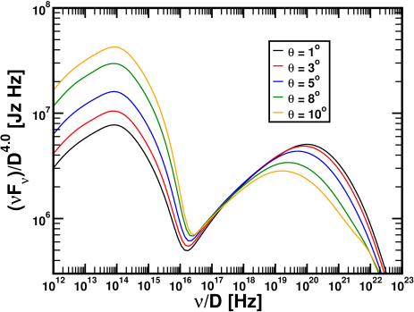
Figure 5: Left panel: same as left panel of Fig. 4, but dividing the frequencies by ${\cal D}$ and the SED by ${\cal D}^{3}$. Right panel: same as right panel of Fig. 4, but normalizing the SED by ${\cal D}^{4}$.

3.3 Strongly magnetized models

The third model family considers the strongly magnetized models where $\sigma_{L}=1$ and $\sigma_{R}=0.1$. The left panel of Fig. 6 shows the dependence of the average spectra on $\Delta g$. Strongly magnetized models in moderately relativistic flows (i.e., having moderate values of $\Gamma_{R}$) dramatically suppress the IC spectral component. However, with increasing values of $\Delta g$ the IC component broadens in frequency range and grows moderately. Another remarkable fact of strongly magnetized models is that for $\Delta g>1.0$ the synchrotron spectrum ceases to be a parabolic, single-peaked curve and becomes a more complex curve where the contributions from the FS and the RS are separated, since the peak frequencies of the synchrotron radiation produced at the FS and at the RS differ by two or three orders of magnitude. The reason is the strong magnetic field in the emitting regions: magnetization in the shocked regions increases proportionally to their compression factors $r_{f}$ and $r_{r}$, respectively (see Eq. 3 in Appendix A), i.e. the shocked regions are even more magnetically dominated than the initial shells. In Table 4 we see that the electrons in the reverse shock of the strongly magnetized models are fast-cooling. In fact, for $\Delta g\gtrsim 1.5$ the injected electron spectrum is almost mono-energetic. In these models the lower cutoff $\gamma_{1r}$ is about a factor of $30$ larger than $\gamma_{1f}$. Since the synchrotron maximum of the fast-cooling electrons is determined by the lower cutoff, the synchrotron spectrum of the RS peaks at a frequency which is $(\gamma_{1f}/\gamma_{1r})^{2}\approx 10^{3}$ times higher than that of the FS. This can be seen in left panel of Fig. 6, where dashed and dot-dashed lines show the respective spectra of the RS and FS of the model S-G10-D2.0-T5.

The dominance of the EIC component for $\Gamma_{R}\gtrsim 20$ and $\nu\gtrsim 10^{21}$ Hz appears to be a property tightly related to the increment of $\Gamma_{R}$ (right panel of Fig. 6). In this case, the EIC component “replicates” the synchrotron peak associated to the forward shock of the collision, modulated by the Klein-Nishina cut-off for large values of $\Gamma_{R}$. Because of this effect, progressively larger values of $\Gamma_{R}$ increase the Compton dominance, i.e. the trend is to recover the standard double-hump structure of the SED as $\Gamma_{R}$ rises. We have tested that for $\Gamma_{R}=50\mbox{ and }100$, the IC spectral component becomes almost monotonic and concave (Fig. 7). For $\Gamma_{R}\gtrsim 50$, the SED becomes akin to that of models with moderate or low shell magnetization, but the IC spectrum displays a plateau rather than a maximum. As the Lorentz factor increases ($\Gamma_{R}\gtrsim 50$), our models form a flat spectrum in the soft X-ray band rather than a minimum between two concave regions. We note that the spectrum of the $\Gamma_{R}=100$ model displays very steep rising spectrum flanking the IC contribution because we have fixed a value of the microphysical parameter $a_{\rm acc}=10^{6}$. Smaller values of such parameter tend to broaden significantly both the IC and the synchrotron peak (Böttcher & Dermer, 2010, see e.g.,). Hence, we foresee that a suitable combination of microphysical and kinematical parameters would recover a more “standard” double-hump structure.

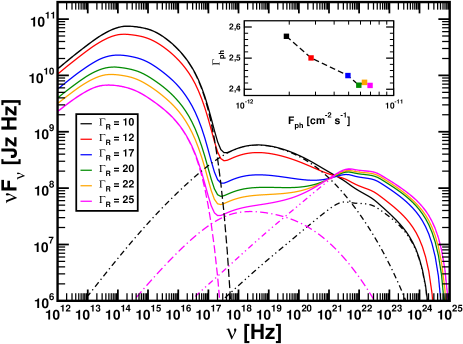
Figure 6: Left panel: same as left panel of Fig. 2, but for the strongly magnetized models S-G10-T5, i.e., $\sigma_{L}=1$ and $\sigma_{R}=0.1$. For the cases $\Delta g=0.5,2.0$ we show the reverse and forward shock contributions to their spectra in dashed and dot-dashed lines, respectively. While at small values of $\Delta g$ the contribution of the RS dominates fully the spectrum, at larger values of $\Delta g$ the FS contribution has increased relative to the RS one, and is an order of magnitude stronger than the former one in the case of the model with $\Delta g=0.5$. This also explains a second (higher) peak in the synchrotron domain, as well as a flattening in the $\gamma$-ray band. Right panel: same as right panel of Fig. 3, but for strongly magnetized models S-D1.0-T5.

$\Delta g$	$\Gamma$	$r_{r}$	$\displaystyle{\frac{B_{r}}{1{\rm G}}}$	$\displaystyle{\frac{Q_{r,11}}{{\rm cm}^{-3}{\rm s}^{-1}}}$	$\displaystyle{\frac{\gamma_{1r}}{10^{2}}}$	$\displaystyle{\frac{\gamma_{2r}}{10^{4}}}$	$\displaystyle{\frac{t^{\prime}_{crr}}{10^{3}{\rm s}}}$	$\displaystyle{\frac{\gamma_{cr}}{\gamma_{1r}}}$	$r_{f}$	$\displaystyle{\frac{B_{f}}{1{\rm G}}}$	$\displaystyle{\frac{Q_{f,11}}{{\rm cm}^{-3}{\rm s}^{-1}}}$	$\displaystyle{\frac{\gamma_{1f}}{10^{2}}}$	$\displaystyle{\frac{\gamma_{2f}}{10^{4}}}$	$\displaystyle{\frac{t^{\prime}_{crf}}{10^{3}{\rm s}}}$	$\displaystyle{\frac{\gamma_{cf}}{\gamma_{1f}}}$
$0.5$	$12.7$	$1.26$	$53.51$	$0.11$	$0.66$	$0.64$	$34.6$	$0.12$	$1.89$	$51.57$	$3.30$	$1.91$	$0.65$	$37.5$	$0.04$
$0.7$	$12.8$	$1.46$	$54.72$	$1.03$	$2.29$	$0.63$	$34.1$	$0.03$	$1.93$	$52.68$	$4.20$	$2.14$	$0.64$	$36.7$	$0.04$
$1.0$	$13.0$	$1.75$	$55.84$	$7.33$	$7.25$	$0.62$	$33.6$	$0.01$	$1.98$	$53.90$	$5.45$	$2.41$	$0.63$	$35.8$	$0.03$
$1.5$	$13.2$	$2.22$	$56.63$	$68.00$	$26.38$	$0.62$	$32.9$	$0.003$	$2.02$	$55.22$	$7.14$	$2.73$	$0.63$	$34.8$	$0.03$
$2.0$	$13.3$	$2.67$	$56.82$	$112900.75$	$61.68$	$0.62$	$32.5$	$0.001$	$2.05$	$56.03$	$8.39$	$2.94$	$0.62$	$34.3$	$0.02$

Table 4: Same as Table 2, but for models S-G10-T5. Note that the $Q_{r,11}$ for $\Delta g=2.0$ is much larger than $Q_{r,11}$ of the other models because $\gamma_{1r}$ is very close to $\gamma_{2r}$.

We also find that the SED of strongly magnetized models is very sensitive to relatively small variations of magnetization between colliding shells. To show such a variety of phenomenologies, we display in Fig. 8 the SEDs of the families S1-G10-T5 (left panel) and S2-G10-T5, right panel, i.e., considering only the variations in the SED induced by a change in $\Delta g$. The three families of strongly magnetized models only have differences in magnetization within a factor 10. Clearly, when the faster shell is less magnetized than the slower one (the case of the S2-family), the models recover a more typical double-hump structure, closer to that found in actual observations. We note that for contribution to the SED of the forward shock in the S2-family is either non-existing, because these models do not form a FS or, if a FS forms, it is very weak (see dashed lines in the right panel of Fig. 8.

For completeness, we consider how the SED changes when varying the viewing angle (Fig. 9). In these models, increasing $\theta$ lowers the total emitted flux all over the spectral range under consideration. The Compton dominance for $\theta\mathbin{\lower 3.0pt\hbox{$\hbox to0.0pt{\raise 5.0pt\hbox{$\char 60\relax$}\hss}\mathchar 29208\relax$}}8^{\circ}$ remains constant. To explain this behavior, we shall note that fixing both $\Gamma_{R}$ and $\Delta g$, increasing $\theta$ is equivalent to decrease the Doppler factor ${\cal D}$. Theoretically, it is known that the beaming pattern of a relativistically moving blob of electrons that Thompson-scatters photons from an external isotropic radiation field changes as ${\cal D}^{4+\alpha}$ ($\alpha$ being the spectral index of the radiation), while the beaming pattern of radiation emitted isotropically in the blob frame (e.g., by synchrotron and SSC processes), changes as ${\cal D}^{3+\alpha}$ (Dermer, 1995). Left and right panels in Fig. 10 show the spectra from Fig. 9 normalized to ${\cal D}^{3}$ and ${\cal D}^{4}$, respectively. Thus, we expect that the reduction of the Doppler factor results in a larger suppression of the IC part of the SED, only if it is dominated by the EIC contribution, as compared with the dimming of the synchrotron component. In the models at hand (S-G10-D1.0), the IC spectrum is dominated by the SSC component, and thus, reducing $\theta$ simply decreases the overall luminosity.

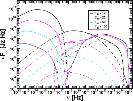
Figure 7: Same as Fig. 6, bur for high $\Gamma_{R}$ cases. For each model the synchrotron, SSC and EIC contributions are shown using dashed, dot-dashed and dot-dot-dashed lines, respectively.

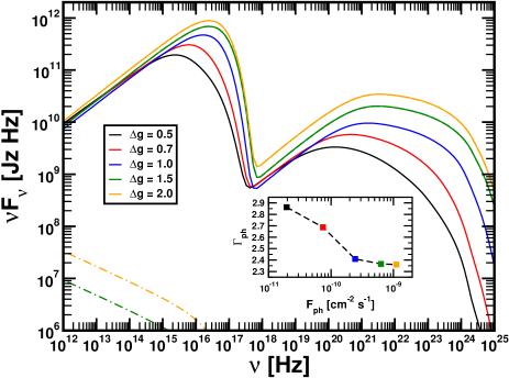
Figure 8: Left: Same as the left panel of Fig. 6 for the family S1-G10-T5. Right: Same as the left panel of Fig. 6 for the family S2-G10-T5. In the S2-family, the forward shock is either non-existing (for $\Delta g\lesssim 1.5$) or extremely weak. We add in the figure the contribution to the spectrum of the forward shocks of the models with $\Delta g=1.5,2$. Note the difference in the stencil of the vertical axis with respect to the left panel.

Figure 9: Same as Fig. 4, but for strongly magnetized models S-G10-D1.0.

Figure 10: Left panel: same as Fig. 9, but normalizing the SED by ${\cal D}^{3}$. Right panel: same as Fig. 4, but normalizing the SED by ${\cal D}^{4}$.

4 Discussion and conclusions

We have extended the survey of parameters started in MA12 for the internal shocks scenario by computing the multi-wavelength, time-dependent emission for several model families chiefly characterized by the magnetization of the colliding shells. In this section we provide a discussion and a summary of our results.

4.1 Intrinsic parameters and emission

In what follows, we consider the effect that changes in intrinsic jet parameters (magnetization, $\Delta g$ and $\Gamma_{R}$) have on the observed emission.

4.1.1 Influence of the magnetic field

As was discussed in Sec. 6.1 of MA12, the main signature of high magnetization is a drastic decrease of the SSC emission due to a much smaller number density of scattering electrons (Eq. 1). As will be stated in Sec. 4.1.3, this decrease can be offset by increasing the bulk Lorentz factor (at a cost of decreasing the overall luminosity). However, extremely relativistic models (from a kinematical point of view), tend to form plateaus rather than clear maxima in the synchrotron and IC regimes, and display relatively small values of $\Gamma_{\rm ph}$. Indeed, the photon spectral index manifest itself as a good indicator of the flow magnetization. Values of $\Gamma_{\rm ph}\gtrsim 2.6$ result in models where the flow magnetization is $\sigma\simeq 10^{-2}$, while either strongly or weakly magnetized shell collisions yield $\Gamma_{\rm ph}\lesssim 2.5$. The observed degeneracy we have found in the case of strongly magnetized and very high Lorentz factor shells is a consequence of the fact that either raising the magnetization or the bulk Lorentz factor, the emitting plasma enters in the ultrarelativistic regime. Which of the two parameters determines most the final SED, depends on the precise magnitudes of $\sigma$ and $\Gamma$.

Another way to correlate magnetization with observed properties can be found representing the Compton dominance $A_{C}$ as a function of the ratio of IC-to-synchrotron peak frequencies $\nu_{IC}/\nu_{syn}$ (see App. B). Models with intermediate or low magnetization occupate a range of $A_{C}$ roughly compatible with observations, while the strongly magnetized models tend to have values of $A_{C}$ hardly compatible with those observed in actual sources, unless collisions in blazars happen at much larger Lorentz factors than currently inferred (see Sect. 4.3).

4.1.2 Influence of $\Delta g$

$\Delta g$ is a parameter which indicates the magnitude of the velocity variations in the jet. From the average spectra shown in the left panels of Figs. 2, 3 and 6 we see that the increase of $\Delta g$ leads to the increase of the Compton dominance parameter (see also Fig. 11), the effect being more important for either weakly or moderately magnetized models than for strongly magnetized ones (for which the Compton dominance is almost independent of $\Delta g$, or even $A_{C}$ decreases for large values of that parameter). Furthermore, the total amount of emitted radiation also increases with increasing $\Delta g$, as is expected from the dynamic efficiency study (Mimica & Aloy, 2010), and confirmed by the radiative efficiency study of MA12. Finally, for low values of $\Delta g$ the EIC emission is either dominant or comparable to the SSC one, while SSC becomes dominant at higher $\Delta g$.

Looking at the physical parameters in the emitting regions (Tables 2, 3 and 4), we see that the increase in $\Delta g$ leads to the increase in the compression factor $r_{f}$ and $r_{r}$ of the FS and RS. The effect is strongest for the weakly magnetized models. This increase has as a consequence the increase in the number density of electrons injected at both, the FS and the RS. A similar argument can be made for the magnetic fields in the emitting regions, since the magnetic field undergoes the shock compression as well (see Appendix A).

In the insets of left panels of Figs. 2, 3 and 6 we see that in $\gamma$-rays the increase of $\Delta g$ generally reflects in the increase of the photon flux and a decrease of the spectral slope $\Gamma_{\rm ph}$. Because of the sensitivity of the photon spectral index in the $\gamma-$ray band, we foresee that the change in $\Gamma_{\rm ph}$ can be a powerful observational proxy for the actual values of $\Delta g$ and a distinctive feature of magnetized flows. Comparing equivalent weakly (Fig. 2; left) and moderately magnetized models (Fig. 3; left), we observe that the maximum $\Gamma_{\rm ph}$ as a function of $\Delta g$ increases by $\sim 15\%$ due to the increase in magnetization, and the value of $\Delta g$ for which the maximum $\Gamma_{\rm ph}$ occurs also grows, at the same time that $F_{\rm ph}$ decreases by a factor of 50.

We have also found that sufficiently large values of $\Delta g$ tend to produce a double-peaked structure in the synchrotron dominated part of the SED. When the relative difference of Lorentz factors grows above $\sim 1.5$, the contributions arising from the FS and the RS shocks peak at different times, the RS contribution lagging behind the FS contribution and being more intense, and occurring at larger frequencies than the latter. The reason for this phenomenology can be found looking at Tab.  4 and noting that $\gamma_{1r}$ becomes very large and comparable to $\gamma_{2r}$ for $\Delta g\mathbin{\lower 3.0pt\hbox{$\hbox to0.0pt{\raise 5.0pt\hbox{$\char 62\relax$}\hss}\mathchar 29208\relax$}}1.5$. For these models $\gamma_{1r}\gg\gamma_{1f}$ and the frequency of the RS spectral peak is almost $10^{3}$ times larger than the frequency of the FS spectral peak. The effect is the flattening of the synchrotron spectrum, or even an appearance of a second peak. This trend is even more clear when the magnetization of the shells is increased, so that the most obvious peak in the UV domain happens for strongly magnetized models (compare the left panels of Figs. 2, 3 and 6). The observational consequences of the appearance of this peak are discussed below (Sect. 4.3).

4.1.3 Influence of $\Gamma_{R}$

$\Gamma_{R}$ is the parameter which determines the bulk Lorentz factor of the jet flow, to a large extent. From Eq. 1 we see that the increase in $\Gamma_{R}$ leads to a decrease of the number density in the shells, a trend which is seen in the right panels of Figs. 2, 3 and 6, since it reduces the emitted flux. Another effect is the decrease in dominance of SSC over EIC as $\Gamma_{R}$ increases. A related feature is the flattening of the $\gamma$-ray spectrum (see figure insets). A consequence of the increasing importance of the EIC is the shifting of the IC spectral maximum to higher frequencies, until the Klein-Nishina limit is reached. For moderately magnetized models (right panel of Fig. 3) the IC maximum becomes independent of $\Gamma_{R}$.

The IC emission in the strongly magnetized models (right panel of Fig. 6) is dominated by SSC for low values of $\Gamma_{R}$. However, as $\Gamma_{R}$ is increased, the higher-frequency EIC component becomes ever more luminous. While none of the models in Fig. 6 reproduces the prototype double-peaked structure of blazar spectra, the increase of the EIC component with $\Gamma_{R}$ indicates that perhaps larger values of $\Gamma_{R}$ might produce a blazar-like spectrum. We have shown in Fig. 7 that the average spectra for strongly magnetized models where $\Gamma_{R}$ is allowed to grow up to $100$ display again a double-peaked spectrum, albeit with a much lower luminosity than the models with lower bulk Lorentz factors.

4.1.4 External radiation field

In this work we did not consider the sources of external radiation in such a detail as was recently done by e.g. Ghisellini & Tavecchio (2009). These authors show that, for a more realistic modeling of the external radiation field, the IC component might be dominating the emission even for a jet with $\sigma\simeq 0.1$. We note, however, that the difference between their and our approach is that we model the magnetohydrodynamics of the shell collision, while they concentrate on more accurately describing the external fields. In our model the magnetic field not only influences the cooling timescales of the emitting particles, but also the shock crossing timescales, making direct comparison difficult, especially for $\sigma\gtrsim 1$ where the dynamics changes substantially (see, e.g., MA12).

In our models, we take a monochromatic external radiation field with a frequency $\nu_{\rm ext}$ in the near infrared band, and with an energy density $u_{\rm ext}$ that tries to mimic, in a simple manner, the emission from a dusty torus or the emission from the broad line region. More complex modeling, such as that introduced by Giommi et al. (2012) can be incorporated in our analysis, at the cost of increasing the number of parameters in our set up.

4.2 The effect of the observing angle

Increasing $\theta$ results in a Doppler deboosting of the collision region and a significant reduction of the observed flux. The decrease of the flux comes along with a moderate decrease of $\Gamma_{\rm ph}$ explained by the different scaling properties with the Doppler factor of the SSC and EIC contributions to the SED. From theoretical grounds, one expects that the synchrotron and SSC contributions to the SED scale as ${\cal D}^{3}$ for, while ${\cal D}^{4}$ is the correct scaling for the EIC spectral component. Such a theoretical inference is based on assuming a moving spherical blob of relativistic particles. In our case, instead a blob we have a pair of distinct cylindrical regions moving towards the observer. The practical consequence of such a morphological difference is that the synchrotron radiation is roughly emitted isotropically, and thus, it scales as ${\cal D}^{3}$ (left panels of Figs. 5 and 10), but the IC contributions are no longer isotropic and thus do not scale either as ${\cal D}^{3}$ nor as ${\cal D}^{4}$. The effect is exacerbated when strong magnetizations are considered (compare the right panels of Figs. 5 and 10).

4.3 Comparison with observations

It has been found in several blazar sources that their SEDs have more than two peaks. Particularly, in some cases a peak frequency of $\sim 10^{15}~{}\mathrm{Hz}$ (e.g., Lichti et al., 1995; Pian et al., 1999) is seen (a UV bump), which is assumed to come purely from the optically thick accretion disk (OTAD) and from the Broad Line Region (BLR). In recent works, thermal radiation from both OTAD and BLR are considered separately in order to classify blazars (Giommi et al., 2012; Giommi et al., 2013). In the present work, we have shown that a peak in the UV band can arise by means of non-thermal and purely internal jet dynamics. This “non-thermal” blue bump is due to the contribution to the SED of the synchrotron radiation from the reverse shock in a collision of shells with a sufficiently large relative Lorentz factor (see left panels of Figs. 2,  3 and 6). We suggest that such a secondary peak in the UV domain is an alternative explanation for the thermal origin of the UV bump. In Giommi et al. (2012), the prototype sources displayed in their Fig. 1 all have synchrotron and IC components of comparable luminosity. In our case, the strength of the UV peak is larger for the models possessing the strongest magnetic fields. In such models, the IC part of the spectrum is strongly suppressed and, thus, they are not compatible with observations. However, moderate magnetization models display synchrotron and IC components of similar luminosity. In addition, an increase in the relative Lorentz factor of the interacting shells produces UV bumps which are more obvious and with peaks shifted to the far UV. According to Giommi et al. (2012), the spectral slope at frequencies below the UV-bump ranges from $\alpha_{\rm r-BlueBump}\sim 0.4$ to $\sim 0.95$. We cannot directly compute such slope from our data, since we have limited ourselves to compute the SED above $10^{12}\,$Hz. However, we find compatibility between our models and observations from comparison of the spectral slope at optical frequencies, where it is smaller than in the whole range $[5\,{\rm GHz},\nu_{\rm BlueBump}]$. Extrapolating the data from our models, values $\Delta g\gtrsim 1.5$ combined with shell magnetizations $\sigma\simeq 10^{-3}$ could accomodate UV bumps with peak frequencies and luminosities in the range pointed out by current blazar observations.

It has to be noted that the intergalactic medium absorption at frequencies between $\sim 3\times 10^{15}\,$Hz and $\sim 3\times 10^{17}\,$Hz is extremely strong, and is not incorporated into our models. Such an extrinsic suppression of the emitted radiation will impose a (redshift-dependent) upper limit to the position of the observed UV peak, below the intrinsic reverse shock synchrotron peaks of our moderately and strongly magnetized models (see e.g., orange line in the left panel of Fig. 6 which peaks at $\sim 10^{17}\,$Hz). In other words, due to the absorption we expect the observed RS synchrotron peak of such a spectrum to appear at UV frequencies (instead of in X-rays), thus providing an alternative explanation for the UV bump.

The current observational picture shows that there are two types of blazar populations with notably different properties. Among other, type defining, properties that are different in BL Lacs and in FSRQ objects we find that their respective synchrotron peak frequencies $\nu_{syn}$ are substantially different. BL Lacs have synchrotron peaks shifted to high frequencies, in some cases above $10^{18}\,$Hz (e.g., Mkn 501). In contrast, FSRQs are strongly peaked at low energies (the mean synchrotron frequency peak is $\bar{\nu}_{syn}\simeq 10^{13.1}$; Giommi et al. 2012).

For the typically assumed or inferred values of the Lorentz factor in blazars (namely, $\Gamma<30$), the locus of models with different magnetizations is different in the $A_{C}$ vs $\nu_{syn}$ graph (Fig. 11). While weakly magnetized models display $A_{C}\gtrsim 3$, the most magnetized ones occupy a region $A_{C}\lesssim 0.1$. In between ($0.1\lesssim A_{C}\lesssim 3$) we find the models with moderate magnetizations ($\sigma\simeq 10^{-2}$). Moreover, we can classify the weakly magnetized models as IC dominated with synchrotron peak in the IR band. According to observations (Finke, 2013; Giommi et al., 2012), this region is occupied by FSRQs, while the moderately magnetized cases fall into the area compatible with data from BL Lacs.

Strongly magnetized models are outside of the observational regime. However, the quite obvious separation of the locus of sources with different magnetizations is challenged when very large values of the slowest shell Lorentz factor ($\Gamma_{R}\gtrsim 30$) are considered. The path followed by models of the family S-D1.0-T5 (red dash-dotted line in the lower part of Fig. 11), heads towards the region of the graph filled by the weakly magnetized models as $\Gamma_{R}$ is increased. This increase of $A_{C}$ corresponds to the fact we have already pointed before: there is a degeneracy between increasing magnetization and increasing Lorentz factor (Fig. 7). Higher values of $\Gamma_{R}$ yield more luminous EC components, making that strongly magnetized models recover the typical SED of blazars, tough with a much smaller flux than unmagnetized models.

Comparing our Fig. 11 with Fig. 5 of Finke (2013), we find that the Compton dominance is a good measurable parameter to correlate the magnetization of the shells with the observed spectra. Moderately magnetized models are located in the region where some BL Lacs are found, namely, with $0.1\lesssim A_{C}\lesssim 1$ and $10^{14}\,{\rm Hz}\lesssim\nu_{syn}\lesssim 10^{16}\,$Hz. We also find that models with high and uniform magnetization ($\sigma_{L}=\sigma_{R}=0.1$; S1-G10-T5 family), and large values of the relative Lorentz factor $\Delta g\gtrsim 1$ (dot-dot-dashed lines in Fig. 11 and orange lines and symbols in Fig. 12), may account for BL Lacs having peak synchrotron frequencies in excess of $10^{16}\,$Hz and $A_{C}\lesssim 0.1$. There is, however, a region of the parameter space which is filled by X-ray peaked synchrotron blazars with $0.1\lesssim A_{C}\lesssim 1$ that we cannot easily explain unless seemingly extreme values $\Delta g\gtrsim 2$ are considered. We point out that the most efficient way of shifting $\nu_{syn}$ towards larger values is increasing $\Delta g$. Such a growth of $\nu_{syn}$ comes with an increase in the Compton dominance, as is found observationally for FSRQ sources (Finke, 2013). Comparatively, varying $\Gamma_{R}$ drives moderate changes in $\nu_{syn}$, unless extreme values $\Gamma_{R}\gtrsim 50$ are considered. We must also take into account that the synchrotron peak frequency is determined by the high-Lorentz factor cut-off $\gamma_{2}$. Most of our models display values $\gamma_{2}\gtrsim 10^{4}$ in the emitting (shocked) regions. For comparison, in Finke (2013) $\gamma_{2}=10^{6}$ is fixed for all his models. The small values of $\gamma_{2}$ in our shell collisions are due to the microphysical parameters we are using, in particular, our choice of the shock acceleration efficiency $a_{\rm acc}$, which was motivated by Böttcher & Dermer (2010). For the models and parameters picked up by Böttcher & Dermer (2010), they find that neither the peak synchrotron frequency, nor the peak flux were sensitively dependent on the choice of $a_{\rm acc}$ (if the power-law Lorentz factor index $q>2$). However, $\gamma_{2}$ shows the same dependence on $a_{\rm acc}$ than on the magnetic field strength: $\gamma_{2}\simeq 4.6\times 10^{7}(a_{\rm acc}B[{\rm G}])^{-0.5}$. In practice, thus, we find a degeneracy in the dependence on both $a_{\rm acc}$ and $B$ for our models.

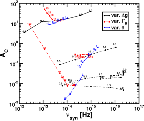
Figure 11: Compton dominance $A_{C}$ as a function of the synchrotron peak frequency $\nu_{\rm syn}$ for the three families of models corresponding to collisions of the three kinds of magnetized shells. We also display the Compton dominance for the families of strongly magnetized models S1 and S2. The different lines are drawn to show the various trends when considering models where we vary a single parameter and keep the rest constant. The variation induced by the change in $\Delta g$, $\Gamma_{R}$ and $\theta$ is shown with black, red and blue lines, respectively. The numbers denote the value of the varied parameter and the line type is associated to the magnetization, corresponding the solid, dashed and dot-dashed lines to weakly, moderately and strongly magnetized shells, respectively. Double-dotted-dashed and dotted-double-dashed lines correspond to the additional models of the families S1-G10-T5 and S2-G10-T5, respectively.

Considering the location of the strongly magnetized models with $\sigma_{L}=1$, and $\sigma_{R}=0.1$ in the $A_{C}$ vs $\nu_{syn}$ graph (Fig. 11), they appear as only marginally compatible with the observations of Finke (2013) , where almost all sources have $A_{C}>10^{-2}$. since in such models is difficult to obtain $A_{C}>10^{-2}$, unless the microphysical parameters of the emitting region are changed substantially (e.g., lowering $a_{\rm acc}$). This seems to indicate that strongly magnetized models with sensitively different magnetizations of the colliding shells (in our case there is a factor 10 difference between the magnetization of the faster and of the slower shell) are in the limit of compatibility with observations, and that even larger magnetizations are banned by data of actual sources. MA12 found that the combination $\sigma_{L}=1$, $\sigma_{R}=0.1$, brings the maximum dynamical efficiency in shell collisions ($\sim 13\%$), and that has been the reason to explore the properties of such models here. Models with large and uniform magnetization $\sigma_{L}=\sigma_{R}=0.1$ display a dynamical efficiency $\sim 10\%$, quite close to the maximum one for a single shell collision, and clearly bracket better the observations in the $A_{C}$ vs $\nu_{syn}$ plane.

The family of S2-models with $\sigma_{L}=0.1$, $\sigma_{R}=1$ is complementary to the S-family, but in the former case, only a RS exists, since the FS turns into a forward rarefaction (MA12), if $\Delta g\lesssim 1.5$. These models possess a larger Compton dominance ($10^{-2}\lesssim A_{C}\lesssim 4\times 10^{-2}$) than those of the S-family (Fig. 11), and their locus in the $F_{\rm ph}$ vs $\Gamma_{\rm ph}$ plane (Fig.12; green line and symbols) is much more compatible with observations. Since the synchrotron emission of the S2-family is only determined by the RS, if $\Delta g\lesssim 1.5$, or dominated by the RS emission if $\Delta g\gtrsim 1.5$, the synchrotron peak tends to be at higher frequencies than in the S and S1 families.

The value of $\Gamma_{\rm ph}$ has also been useful to differentiate observationally between BL Lacs and FSRQs. According to Abdo et al. (2010) the photon index, provides a convenient mean to study the spectral hardness, which is the ratio between the hard sub-band and the soft sub-band (Abdo et al., 2009). In Fig. 12 we compare the values of $\Gamma_{\rm ph}$ computed for our three families of models with actual observations of FSRQs and BL Lacs from the 2LAG catalog (Ackermann et al., 2011). We only represent values of such catalog corresponding to sources with redshifts $0.4\leq z\leq 0.6$, since our models have been computed assuming $z=0.5$. We note that the values of $\Gamma_{\rm ph}$ calculated from fits of the $\gamma-$ray spectra in our models with moderate magnetization (red colored in the figure) fall just above the observed maximum values attained in FSRQs ($\Gamma_{\rm ph,obs}^{\rm FSRQ}\lesssim 2.6$), if the Lorentz factor of the slower shell is $\Gamma_{R}\sim 10$. However, models with moderate magnetization and larger Lorentz factors $\Gamma_{R}\gtrsim 15$ display photon indices fully compatible with FSRQs and photon fluxes in the lower limit set by the technical threshold that prevents Fermi to detect sources with $F_{\rm ph}\lesssim 2\times 10^{-10}\,$photons cm^-2 s^-1. BL Lacs exhibit even flatter $\gamma-$ray spectra than FSRQs, with observed values of the photon index $\Gamma_{\rm ph,obs}^{\rm BLLac}\lesssim 2.4$. Values $\Gamma_{\rm ph}\gtrsim 2$ are on reach of both strongly or weakly magnetized models. Nevertheless, the photon flux of strongly magnetized models falls below the current technical threshold. Being conservative, this under-prediction of the gamma-photon flux could be taken as a hint indicating that only models with small or negligible magnetization can reproduce properly the properties of FSRQs, LBL, and perhaps IBL sources, while HBL and BL Lacs have microphysical properties which differ from the ones parametrized in this work. According to Abdo et al. (2009), the photon index is a quantity that could constrain the emission and acceleration processes that may be occurring within the jet that produce the flares at hand. Particularly, we have fixed a number of microphysical parameters ($\epsilon_{B}$, $\epsilon_{e}$, $a_{\rm acc}$, etc.) to typically accepted values, but we shall not disregard that X-ray, synchrotron-peaked sources have different values of the aforementioned microphysical parameters. On the other hand, our values of $\Gamma_{\rm ph}$ are not fully precise, the reason being the approximated treatment of the Klein-Nishina cutoff. Being not so conservative, we may speculate that our current gamma ray detectors cannot observe sources with sufficiently small flux ($F_{\rm ph}\lesssim 3\times 10^{-11}\,$photons cm^-2 s^-1) to discard or confirm that strongly magnetized blazars may exist.

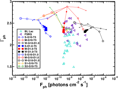
Figure 12: Comparison between our numerical models and those sources (FRSQs and BL Lacs) whose redshift is $0.4\leq z\leq 0.6$ in the 2LAG catalog (Ackermann et al., 2011). The size of the symbols associated to our models grows as the parameter which is varied does. For instance, in the case of models M-G10-D1.0, the smaller values of $\theta$ correspond to the smaller red circles in the plot.

4.4 Conclusions and future work

In the standard model, the SEDs of FSRQs and BL Lacs can be fit by a double parabolic component with maxima corresponding to the synchrotron and to the inverse Compton peaks. We have shown that the SEDs of FSRQs and BL Lacs strongly depends on the magnetization of the emitting plasma. Our models predict a more complex phenomenology than is currently supported by the observational data. In a conservative approach this would imply that the observations restrict the probable magnetization of the colliding shells that take place in actual sources to, at most, moderate values (i.e., $\sigma\lesssim 10^{-1}$), and if the magnetization is large, with variations in magnetization between colliding shells which are smaller than a factor $\sim 10$. However, we have also demonstrated that if the shells Lorentz factor is sufficiently large (e.g., $\Gamma_{R}\gtrsim 50$), magnetizations $\sigma\simeq 1$ (Fig. 7) are also compatible with a doble hump. Therefore, we cannot completely discard the possibility that some sources are very ultrarelativistic both in a kinematically sense and regarding its magnetization.

We find that FSRQs have observational properties on reach of models with negligible or moderate magnetic fields. The scattering of the observed FSRQs in the $A_{C}$ vs $\nu_{syn}$ plane, can be explained by both variations of the intrinsic shell parameters ($\Delta g$ and $\Gamma_{R}$ most likely), and of the extrinsic ones (the orientation of the source). BL Lacs with moderate peak synchrotron frequencies $\nu_{syn}\lesssim 10^{16}\,$Hz and Compton dominance parameter $0.1\gtrsim A_{C}\gtrsim 1$ display properties that can be reproduced with models with moderate and uniform magnetization ($\sigma_{L}=\sigma_{R}=10^{-2}$). HBL sources can be partly accommodated within our model if the magnetization is relatively large and uniform ($\sigma_{L}=\sigma_{R}=10^{-1}$) or if the magnetization of the faster colliding shell is a bit smaller than that of the slower one ($\sigma_{L}=10^{-1},\sigma_{R}=1$). We therefore find that a fair fraction of the blazar sequence can be explained in terms of the intrinsically different magnetization of the colliding shells.

We observe that the change in the photon spectral index ($\Gamma_{\rm ph}$) in the $\gamma-$ray band can be a powerful observational proxy for the actual values of the magnetization and of the relative Lorentz factor of the colliding shells. Values $\Gamma_{\rm ph}\gtrsim 2.6$ result in models where the flow magnetization is $\sigma\sim 10^{-2}$, whereas strongly magnetized shell collisions ($\sigma>0.1$) as well as weakly magnetized models may yield $\Gamma_{\rm ph}\lesssim 2.6$.

The EIC contribution to the SED has been included in a very simplified way in this paper. We plan to improve on this item by considering more realistic background field photons as in, e.g., Giommi et al. (2012). We expect that including seed photons in a wider frequency range will modify the IC spectrum of strongly magnetized models or of models with low-to-moderate magnetization, but large bulk Lorentz factor. Finally, the microphysical parameters characterizing the emitting plasma have been fixed in this manuscript. In a follow up paper, we will explore the sensitivity of the results (particularly in moderately to highly magnetized models) to variations of the most significant microphysical parameters (e.g., $a_{\rm acc},\epsilon_{B},\epsilon_{e}$, etc).

Appendix A Magnetization in the shocked regions

In an one-dimensional Riemann problem in RMHD the quantity ${\cal B}:=B^{\prime}/\rho$ is constant across shocks and rarefactions (e.g., Romero et al., 2005), where $B^{\prime}$ and $\rho$ are the comoving magnetic field and the fluid density, respectively. The magnetization is defined as

$$\sigma:=\displaystyle{\frac{B^{{}^{\prime}2}}{4\pi\rho c^{2}}}\,,$$ (2)

and can also be written as $\sigma={\cal B}^{2}\rho/(4\pi c^{2})$.

We point out that the inertial mass-density in a cold magnetized plasma is $\rho(1+\sigma)\Gamma^{2}$. This means that the plasma can become ultrarelativistic if either $\sigma\gg 1$ or $\Gamma\gg 1$, since in both cases the inertial mass-density becomes much larger than the rest-mass density $\rho$.

The density in the shocked region can be written as $\rho_{s}=r\rho_{0}$, where $r$ is the compression ratio and $\rho_{0}$ is the density in the unshocked region. Assuming that in the unshocked region the magnetization is $\sigma_{0}$ and using the fact that ${\cal B}$ is a constant we have for the magnetization in the shocked region:

$$\sigma_{S}=\displaystyle{\frac{{\cal B}^{2}\rho_{S}}{4\pi c^{2}}}=\displaystyle{\frac{{\cal B}^{2}r\rho_{0}}{4\pi c^{2}}}=r\sigma_{0}\,.$$ (3)

As can be seen from Eq. 3, the magnetization increases linearly with the shock compression factor.

Appendix B Relation between Compton dominance and $F_{\rm IC}/F_{\rm syn}$

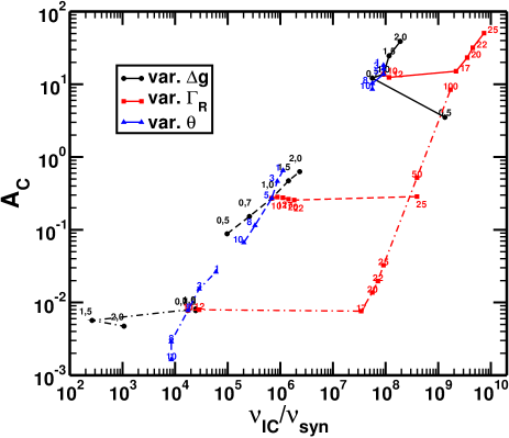
Figure 13: Left: Compton dominance, $A_{C}$, as a function of $\nu_{IC}/\nu_{syn}$. Right: Same as the left panel, but replacing $\nu_{IC}/\nu_{syn}$ by the ratio of peak fluxes $F_{\rm IC}/F_{\rm syn}$. The models and the lines in this figure as the same as in Fig. 11.

In Fig. 13 (left) we present a plot of the Compton dominance parameter as a function of the ratio of peak frequencies $\nu_{IC}/\nu_{syn}$, since these properties can be directly measured from observations. The models under consideration in this work separate according to their respective magnetization. As expected, the lower Compton dominance happens for strongly magnetized models (dot-dashed lines in the figure), while the weakly magnetized shell collisions display the larger $A_{C}$. According to $A_{C}$, there is a factor of more than ten in Compton dominance when considering shells with magnetizations $\sigma\sim 10^{-2}$, as compared with basically unmagnetized models. We also note that models with varying orientation are shifted along diagonal lines in the plot (blue lines in Fig. 13). This is also the case for families of models in which we vary $\Gamma_{R}$ above a threshold (magnetization dependent) such that the IC spectrum is dominated by the EIC contribution (red lines in Fig. 13). If the IC spectrum is dominated by the SSC contribution, changing $\Gamma_{R}$ yields a horizontal displacement in the plot. Models with varying $\Delta g$ display a similar drift as those in which $\theta$ is changed in the case of the moderately magnetized shell collisions. The trend is not so well defined in case of weakly magnetized models, and for strongly magnetized models (S-G10-T5), the Compton dominance is rather insensitive to $\Delta g$, though lower values of $\Delta g$ yield larger values of $\nu_{IC}/\nu_{syn}$.

To study the global trends of the models, MA12 studied the parameter space spanned by the ratio of the IC and synchrotron peak frequencies and the ratio of the IC and synchrotron fluences. In this section we show that the latter ratio, which we denote by $F_{\rm IC}/F_{\rm syn}$ has a very tight correlation with the Compton dominance parameter $A_{C}$, defined as the ratio of the peak IC and peak synchrotron luminosity, as can be seen from Figure 13 (right). This means that either $A_{C}$ or $F_{\rm IC}/F_{\rm syn}$ can be used interchangeably for the purpose of our parametric study.

References

- Abdo et al. (2009) Abdo A. A., Ackermann M., Ajello M., Atwood W. B., Axelsson M., Baldini L., Ballet J., et al. B., 2009, ApJ, 700, 597
- Abdo et al. (2010) Abdo A. A., Ackermann M., Ajello M. Atwood W. B., Axelsson M., Baldini L., Ballet J., Barbiellini G., et al. 2010, ApJ, 710, 1271
- Ackermann et al. (2011) Ackermann M., Ajello M., Allafort A., Antolini E., Atwood W. B., Axelsson M., Baldini L., Ballet J., Barbiellini G., Bastieri D., Bechtol K., Bellazzini R., Berenji B., Blandford R. D., Bloom E. D., et a l., 2011, ApJ, 743, 171
- Aloy & Mimica (2008) Aloy M. A., Mimica P., 2008, ApJ, 681, 84
- Bošnjak et al. (2009) Bošnjak Ž., Daigne F., Dubus G., 2009, A&A, 498, 677
- Böttcher & Dermer (2010) Böttcher M., Dermer C., 2010, ApJ, 711, 445
- Böttcher & Dermer (2002) Böttcher M., Dermer C. D., 2002, ApJ, 564, 86
- Chen et al. (2011) Chen X., Fossati G., Liang E. P., Böttcher M., 2011, MNRAS, 416, 2368
- Daigne et al. (2011) Daigne F., Bošnjak Ž., Dubus G., 2011, A&A, 526, A110
- Daigne & Mochkovitch (1998) Daigne F., Mochkovitch R., 1998, MNRAS, 296, 275
- Dermer (1995) Dermer C. D., 1995, ApJL, 446, L63
- Fan et al. (2004) Fan Y. Z., Wei D. M., Zhang B., 2004, MNRAS, 354, 1031
- Finke (2013) Finke J. D., 2013, ApJ, 763, 134
- Fossati et al. (1998) Fossati G., Maraschi L., Celotti A., Comastri A., Ghisellini G., 1998, MNRAS, 299, 433
- Ghisellini et al. (1998) Ghisellini G., Celotti A., Fossati G., Maraschi L., Comastri A., 1998, MNRAS, 301, 451
- Ghisellini & Tavecchio (2009) Ghisellini G., Tavecchio F., 2009, MNRAS, 397, 985
- Giommi et al. (2013) Giommi P., Padovani P., Polenta G., 2013, ArXiv e-prints
- Giommi et al. (2012) Giommi P., Padovani P., Polenta G., Turriziani S., D’Elia V., Piranomonte S., 2012, MNRAS, 420, 2899
- Giommi et al. (2012) Giommi P., Polenta G., Lähteenmäki A., Thompson D. J., Capalbi M., Cutini S., Gasparrini D., González-Nuevo J., et al. 2012, A&A, 541, A160
- Joshi & Böttcher (2011) Joshi M., Böttcher M., 2011, ApJ, 727, 21
- Kardashev (1962) Kardashev N. S., 1962, SvA, 6, 317
- Kino et al. (2004) Kino M., Mizuta A., Yamada S., 2004, ApJ, 611, 1021
- Kobayashi et al. (1997) Kobayashi S., Piran T., Sari R., 1997, ApJ, 490, 92
- Lichti et al. (1995) Lichti G. G., Balonek T., Courvoisier T. J.-L., Johnson N., McConnell M., McNamara B., von Montigny C., Paciesas W., Robson E. I., Sadun A., Schalinski C., Smith A. G., Staubert R., Steppe H., Swanenburg B. N., Turner M. J. L., et al. 1995, A&A, 298, 711
- Mimica (2004) Mimica P., 2004, Ph.D Thesis- Ludwig-Maximilian-Universität-München, 159 pages
- Mimica & Aloy (2010) Mimica P., Aloy M. A., 2010, MNRAS, 401, 525
- Mimica & Aloy (2012) Mimica P., Aloy M. A., 2012, MNRAS, 421, 2635
- Mimica et al. (2007) Mimica P., Aloy M. A., Müller E., 2007, A&A, 466, 93
- Mimica et al. (2004) Mimica P., Aloy M. A., Müller E., Brinkmann W., 2004, A&A, 418, 947
- Mimica et al. (2005) Mimica P., Aloy M. A., Müller E., Brinkmann W., 2005, A&A, 441, 103
- Pian et al. (1999) Pian E., Urry C. M., Maraschi L., Madejski G., McHardy I. M., Koratkar A., Treves A., Chiappetti L., Grandi P., Hartman R. C., Kubo H., Leach C. M., Pesce J. E., Imhoff C., Thompson R., Wehrle A. E., 1999, ApJ, 521, 112
- Rees & Meszaros (1994) Rees M. J., Meszaros P., 1994, ApJL, 430, L93
- Romero et al. (2005) Romero R., Marti J., Pons J. A., Ibáñez J. M., Miralles J. A., 2005, JFM, 544, 323
- Spada et al. (2001) Spada M., Ghisellini G., Lazzati D., Celotti A., 2001, MNRAS, 325, 1559
- Urry & Padovani (1995) Urry C. M., Padovani P., 1995, PASP, 107, 803
- Zacharias & Schlickeiser (2010) Zacharias M., Schlickeiser R., 2010, A&A, 524, A31