MLI: An API for Distributed Machine Learning

Abstract

MLI is an Application Programming Interface designed to address the challenges of building Machine Learning algorithms in a distributed setting based on data-centric computing. Its primary goal is to simplify the development of high-performance, scalable, distributed algorithms. Our initial results show that, relative to existing systems, this interface can be used to build distributed implementations of a wide variety of common Machine Learning algorithms with minimal complexity and highly competitive performance and scalability.

I Introduction

The recent success stories of machine learning (ML) driven applications have created an increasing demand for scalable ML solutions. Nonetheless, ML researchers often prefer to code their solutions in statistical computing languages such as MATLAB or R, as these languages allow them to code in fewer lines using syntax that resembles high-level pseudocode. MATLAB and R allow researchers to avoid low-level implementation details, leading to quickly developed prototypes that are often sufficient for small scale exploration. However, these prototypes are typically ad-hoc, non-robust, and non-scalable implementations. In contrast, industrial implementations of these solutions often require a relatively heavy amount of development effort and are difficult to change once implemented.

This disconnect between these ad-hoc scripts and the growing need for scalable ML, in particular systems that leverage the increasingly pervasive cloud computing architecture, has spurred the development of several distributed systems for ML. Initial attempts at such systems exposed a restricted set of low-level primitives for development, e.g., MapReduce [1] or graph-based [2, 3] interfaces. The resulting systems are indeed significantly faster and more scalable than MATLAB or R scripts. They also tend to be much less accessible to ML researchers, as ML algorithms do not always naturally fit into the exposed low-level primitives, and moreover, efficient use of these primitives requires a fairly advanced knowledge of the underlying distributed system.

Subsequent attempts at distributed systems have exposed high-level interfaces that compile down to low-level primitives. These systems abstract away much of the communication and parallelization complexity inherent in distributed ML implementations. Although these systems can in theory obtain excellent performance, they are quite difficult to implement in practice, as they either heavily rely on optimizers to effectively transform high-level code into efficient distributed implementations [4, 5], or utilize pattern matching techniques to identify regions that can be replaced by low-level implementations [6]. The need for fast ML algorithms has also led to the development of highly specialized systems for ML using a restricted set of algorithms [7, 8], with varying degrees of scalability.

Given the accessibility issues of low-level systems and the implementation issues of the high-level systems, ML researchers have yet to widely adopt any of the existing systems. Indeed, ML researchers, both in academic and industrial environments, often rely on system programmers to translate the prototypes of their novel, and often subtle, algorithmic insights into scalable and robust implementations. Unfortunately, there is often a ‘loss in translation’ during this process; small misinterpretation and/or minor errors are unavoidable and can significantly impact the quality of the algorithm. Furthermore, due to the randomized nature of many ML algorithms, it is not always straightforward to construct appropriate test-cases and discover these bugs.

Figure 1: Landscape of existing development platforms for ML.

In this paper, we present a novel API for ML, called MLI, to bridge this gap between prototypes and industry-grade ML software. We provide abstractions that simplify ML development in comparison to pure MapReduce and graph-based primitives, while nonetheless allowing developers control of the communication and parallelization patterns of their algorithms, thus obviating the need for a complex optimizer. With MLI, we aim to be in the top right corner of Figure 1, by providing a development environment that is nearly on par with the usability of MATLAB or R, while matching the scalability of and approaching the walltime of low-level distributed systems. We make the following contributions in this work:

MLI: We show how MLI-supported high-level ML abstractions naturally target common ML problems related to data loading, feature extraction, model training and testing.

Usability: We demonstrate that implementing ML algorithms written against MLI yields concise, readable code, comparable to MATLAB or R.

Scalability: We implement MLI on Spark [11], a cluster computing system designed for iterative computation in a large scale distributed setting. Our results with logistic regression and matrix factorization illustrate that MLI/Spark vastly outperforms Mahout and matches the scaling properties of specialized, low-level systems (Vowpal Wabbit, GraphLab), with performance within a small constant factor.

II Related work

The widespread application of ML techniques has inspired the development of new ML platforms with focuses ranging from productivity to scalability. In this section we review a few of the representative projects. It is worth nothing that in many cases MLI is inspired and guided by these earlier efforts.

Systems like MATLAB and R pioneered high-productivity numerical computing. By combining high-level languages tailored to application domains with intuitive interfaces and interactive interpreted execution, these systems have redefined the way scientists and statisticians interact with data. From the database community, projects like MADLib [12] and Hazy [13] have tried to expose ML algorithms in the context of well established systems. Alternatively, projects like Weka [14], scikit-learn [15] and Google Predict [16] have sought to expose a library of ML tools in an intuitive interface. However, none of these systems focus on the challenges of scaling ML to the emerging distributed data setting.

High productivity tools have struggled to keep up with the growing computational, bandwidth, and storage demands of modern large-scale ML. Although both MATLAB and R now provide limited support for multi-core and distributed scaling, they adopt the traditional process centric approach and are not well suited for large-scale distributed data-centric workloads [17, 18]. In the R community, efforts have been made to run R on data-centric runtimes like Hadoop [19], but to our knowledge none have obtained widespread adoption.

Early efforts to develop more scalable tools and APIs for ML focused on specific applications. Systems like liblinear [20], Vowpal Wabbit [8], and Shogun [7] initially focused on linear models, online learning, and kernel methods, respectively. Others, like MLPack [21], started to develop entire collections of learning algorithms optimized for multicore architectures. These efforts lead to highly efficient systems for specialized tasks, but do not directly simplify the design and implementation of new scalable ML methods, and most are not well-suited to distributed learning.

Various methods have leveraged MapReduce platforms like Hadoop to develop distributed ML libraries. Mahout [1] does not simplify the design and development of new ML methods, and its reliance on HDFS to store and communicate intermediate state makes it poorly suited for iterative algorithms. SystemML [4] introduces a low-level algebra which it then compiles to MapReduce jobs. This algebra exposes the opportunity for advanced optimization, but also complicates the system, and SystemML also suffers from Hadoop’s limitations on iterative computation.

Others have sought to generalize the MapReduce computational model. Systems like DryadLinq [22] and Hyracks [23] can efficiently execute complex distributed data-flow operations and express full relational algebras. However, these systems expose low-level APIs and require the ML expert to recast their algorithms as dataflow operators. In contrast, GraphLab [3] is well suited to certain types of ML tasks, its low-level API and focus on graphs makes it challenging to apply to more traditional ML problems. Alternatively, OptiML [6] and SEJITS [24] provide higher level embedded DSLs capable of expressing both graph and matrix operations and compiling those operations down to hardware accelerated routines. Both rely on pattern matching to find regions of code which can be mapped to efficient low-level implementations. Unfortunately, finding common patterns can be challenging in rapidly evolving disciplines like machine learning.

III MLI

With MLI, we introduce mild constraints on the computational model in order to promote the design and implementation of user-friendly, scalable algorithms. Our interface consists of two fundamental objects – MLTable and LocalMatrix – each with its own API. These objects are used by developers to build Optimizers, which in turn are used by Algorithms to produce Models. It should be noted that these APIs are system-independent - that is, they can be implemented in local and distributed settings (Shared Memory, MPI, Spark, or Hadoop). Our first implementation supporting this interface is built on the Spark platform.

These APIs help developers solve several common problems. First, MLTable assists in data loading and feature extraction. While other systems [8, 1, 3, 2] require data to be imported in custom formats, MLTable allows users to load their data in an unstructured or semi-structured format, apply a series of transformations, and subsequently train a model. LocalMatrix provides linear algebra operations on subsets of the fully featurized dataset. By breaking the full dataset into row-wise partitions of the original dataset and operating locally on those partitions, we give the developer access to higher level programming primitives while still allowing them to control the communication that takes place between nodes and reason about the computational complexity of their algorithms.

As part of MLI, we also pre-define a set of common interfaces for Optimization, Algorithms, and Models to encourage code reuse and to ensure a consistent external system interface. In the remainder of this section we describe these abstractions in more detail.

III-A MLTable

MLTable is an object which provides a familiar table-like interface to a developer, and is designed to mimic a SQL table, an R data.frame, or a MATLAB Dataset Array. The basic MLTable API is illustrated in Figure A1. An MLTable is a collection of rows, each of which conforms to the table’s column schema. Each column is of a particular type, optionally has a name, and can be of the following basic types: String, Integer, Boolean, and Scalar (floating point numeric data). Importantly, any cell in the table can be “Empty” and this is represented with a special value. The table interface, which should be familiar to many developers, supports common operations like relational joins, unions, and projections - as well as map and reduce operations on rows which follow similar semantics to other MapReduce systems.

Additionally, tables support batch operations on partitions of the data, which enable parallel data-local operation on multiple data items. While ML algorithms primarily expect numerical data as input, we expose MLTable as an interface for processing the semi-structured, mixed type data that are present in real-world applications, and transforming this raw data into feature vectors for model training. Given this interface, we are able to load structured data into an MLTable, and then apply a series of transformations to the data in parallel to produce input that is suitable for a ML algorithm. By supporting common data integration tasks out of the box in a straightforward and consistent manner, we significantly decrease the amount of time spent during data preparation and feature extraction.

Once data is featurized, it can be cast into an MLNumericTable, which is a convenience type that most ML algorithms will expect as input. The MLNumericTable interface is the same as MLTable, but it guarantees that all columns are numeric, and by convention each row will be treated as a single feature vector.

An example of an end-to-end text clustering pipeline using MLTable is shown in Figure A2. This pipeline consists of nGrams() computation on the raw text input data and subsequent tfIdf() feature extraction. We then perform K-means clustering on the resulting features to produce an output model. This model could be used to make recommendations or as input to downstream analytical processing.

III-B LocalMatrix

At their core, many ML algorithms are concisely expressed using linear algebra operations. For example, the update step in stochastic gradient descent for generalized linear models such as logistic regression, linear regression, etc. involves computing the gradient of a weight vector with respect to a test class and a training point. In the case of logistic regression, this is ultimately the dot product of two vectors, (or a matrix/vector multiplication in the case of mini-batch SGD), followed by a vector/vector subtraction.

LocalMatrix provides these linear algebra primitives but on partitions of data. The partitions of the data presented to the developer are typically automatically determined by the system. That is, we require programmers to develop algorithms such that all operations can be performed locally and later combined via global reduce operations. This re-assembles to a large degree the shared nothing principle from distributed computing and often leads to highly scalable algorithms. We also considered exposing globally distributed linear algebra operations, but explicitly decided against it primarily because global operators would hide the computational complexity and communication overhead of performing these operations. Instead, by offering linear algebra on subsets (i.e., partitions) of the data, we provide developers with a high level of abstraction while encouraging them to reason about efficiency.

Aside from the semantic difference that operations are performed on individual partitions, LocalMatrix is designed to resemble a matrix in MATLAB, R, or most other numerical programming environments. It supports indexing by rows, columns, or slices of each. A LocalMatrix also supports Matrix-Matrix and Matrix-Scalar algebraic operations, and common linear algebra routines like matrix inversion.

III-C Optimization, Models, and Algorithms

In addition to MLTable and LocalMatrix, we provide additional interfaces called Optimizer, Algorithm, and Model.

Many models cannot be solved via closed form solutions, and even when closed-form solutions exist, the computational complexity of these solutions often increases super-linearly with data size, as in the case with basic linear regression. As a result, various optimization techniques are used to converge to an approximate solution while iterating over the data. We treat optimization as a first class citizen in our API, and the system is built to support new optimizers. We refer the reader to our reference implementation for Stochastic Gradient Descent in Figure A4.

Finally, we encourage developers to implement their algorithms using the Algorithm interface, which should return a model as specified by the Model interface. An algorithm implementing the Algorithm interface is a class with a train() method that accepts data and hyperparameters as input, and produces a Model. A Model is an object which makes predictions. In the case of a classification model, this would be a predicted class given a new example point. In the case of a collaborative filtering model, this might be recommendations for an existing user in the system. Both interfaces are rather simple, but crucially help to provide one common interface for developers (and to the MLbase system as a whole).

IV Examples

To evaluate the design claims made in the earlier sections, we evaluate MLI as well as competing ML systems on two representative real-world problems, namely binary classification and matrix factorization. When implementing algorithms against MLI, we chose Spark as our first platform because it is well-suited for computationally intensive, iterative jobs on large datasets that are characteristic of large ML workloads. Moreover, many large-scale ML systems, e.g,  [8, 3] do not emphasize fault tolerance. In contrast, Spark’s resilience properties, due to automatic data replication and computation lineage, are quite attractive in a distributed environments where automatic recovery from node failure is a necessity. Given our choice to build on top of Spark, it was natural for the first implementation of our API to be in Scala.

Our experiments illustrate three attractive features about MLI. First, we show that MLI yields concise and readable code. In the interest of space, here we compare the code length for comparable implementations of algorithms in MATLAB and MLI in the Appendix. Second, we argue that MLI supports a wide variety of algorithms. Although we focus on two problem settings, these examples demonstrate wide-ranging functionality of MLI and in fact naturally extend to a diverse group of ML algorithms, e.g., linear SVMs, linear regression, and (L1, L2, elastic net)-regularized variants therein, simply by changing the expression of the gradient function (and adding a proximal operator in the case of L1-regularization). Third, we demonstrate that the implementations written against MLI are performant and scalable. We present performance results comparing execution times of various systems on our two examples. We further present extensive strong and weak scalability results. Both sets of results show that the implementations in MLI match the scalability of low-level distributed systems with performance within a small constant factor.

System Lines of Code MLI 55 Vowpal Wabbit 721 MATLAB 11
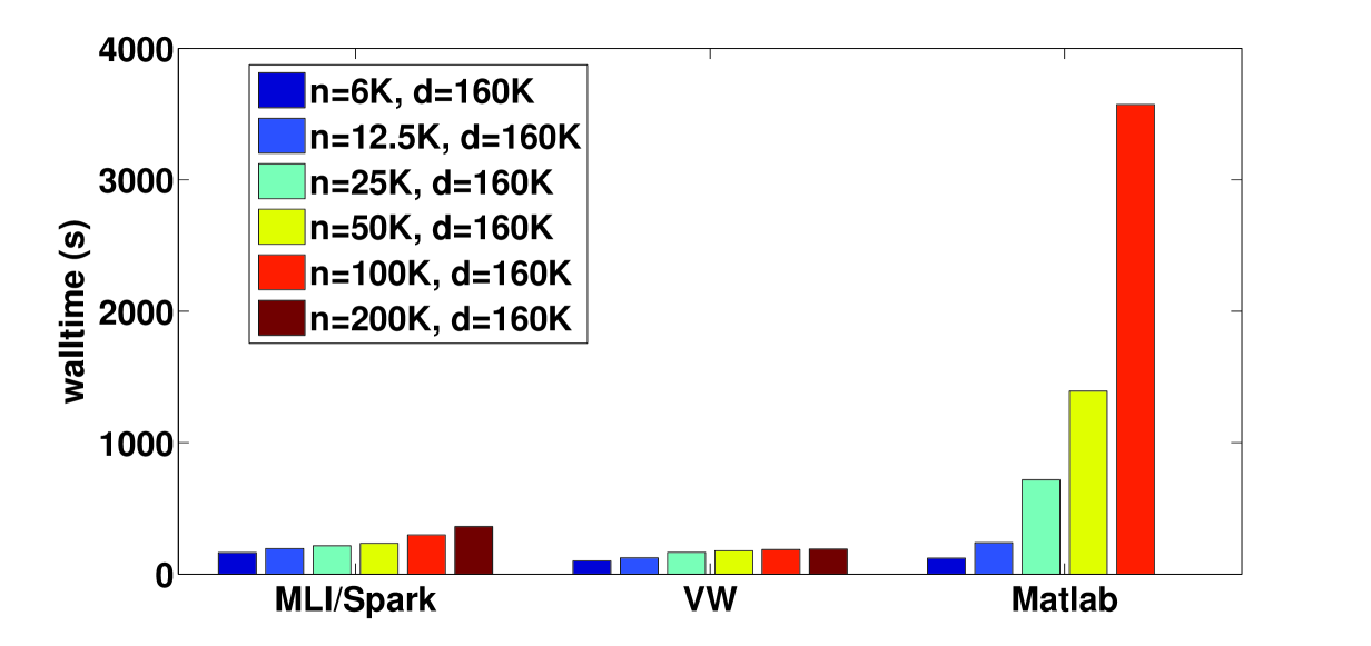
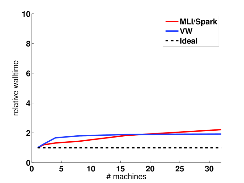
(a)	(b)	(c)

Figure 2: Logistic regression experiments. (a) Lines of code. (b) Execution time for weak scaling. (c) Weak scaling.

IV-A Binary Classification: Logistic Regression

Let $X\in\mathbb{R}^{n\times d}$ be a dataset of $n$ points with $d$ features, $x_{i}\in\mathbb{R}^{d}$ be the $i$th data point, and define $y\in\{0,1\}^{n}$ as the corresponding set of binary labels. Logistic regression is a canonical classification algorithm. The optimal parameter vector $w^{*}\in\mathbb{R}^{d}$ can be found by minimizing the negative likelihood function, $f(w)=-\log p(X|w)$. Taking the gradient of the negative log likelihood, we have:

$$\nabla f=\sum_{i=1}^{n}\bigg{[}\big{(}\sigma(w^{\top}x_{i})-y_{i}\big{)}x_{i}\bigg{]}\,,$$ (1)

where $\sigma(x)=1/(1+\operatorname{exp}\mathopen{}\mathclose{{}\left(-x}\right))$ is the logistic sigmoid function. Gradient descent (GD) is a standard first-order iterative method to solve for $w^{*}$; at the $t$th iteration we move in the direction of the negative gradient with step size controlled by a learning rate, $\eta$, i.e., we set $w_{t+1}=w_{t}-\eta\nabla f$. Stochastic gradient descent (SGD) involves approximating the sum in Equation 1 by a single summand.

Experimental Setup and Data

We run both strong and weak scaling experiments on 1, 2, 4, 8, 16, and 32 machines. All are Amazon m2.4xlarge EC2 instances with 68GB of RAM and 8 virtual cores running in the us1-east region. They are configured using the default Spark 0.7.0 AMI and are running a recent version of Spark and Hadoop 1.0.4. We compare our system to the latest version of Vowpal Wabbit (VW) running on the same cluster, and MATLAB running on a similarly configured (single node) machine. We do not compare against Mahout for these experiments because its implementation of Logistic Regression via SGD is very communication intensive, and we feel that this implementation would not provide a fair comparison for Mahout.

We run our weak scaling experiments on a training set of up to approximately 200GB of featurized ImageNet [25] data where each image is represented with 160K dense features, yielding approximately 200K images total for the 32-node experiment. The number of input points used is proportional to the number of nodes in the cluster for the experiment. We further note that this experiment only represents approximately 20% of the full ImageNet dataset. While we were able to train a full classifier using our system in approximately 2.5 hours, the preprocessing required to prepare the data for VW on the full set of data was too onerous to complete the experiment. In our strong scaling experiments, we train on 5% of this base data for the same number of nodes.

Implementation

We have implemented logistic regression via SGD. To approximate the algorithm used in VW [26] we run SGD locally on each partition before averaging parameters globally. We note, however, that there are several alternative methods to implement SGD on top of MLI. Implementing Logistic Regression in MLI is as simple as defining the form of the gradient function and calling the SGD Optimizer with that function. Additionally, the code that implements StochasticGradientDescent is both short and fairly interpretable.

Algorithmically, our implementation is identical to VW, with one meaningful difference, namely aggregating results across worker nodes after each round. VW uses an “AllReduce” communication primitive to build an aggregation tree when averaging together model parameters after each iteration. It then uses the same tree to broadcast these results back to workers. In contrast, we take a more traditional MapReduce approach and average all parameters at the cluster’s master node at each iteration, then broadcast the parameters to each node using a one-to-many broadcast. As the number of machines increases, VW’s approach is theoretically more efficient from the perspective of communication and parallelizes better with respect to computation. In practice, we see comparable scaling results as more machines are added.

In MATLAB, we implement gradient descent instead of SGD, as gradient descent requires roughly the same number of numeric operations as SGD but does not require an inner loop to pass over the data. It can thus be implemented in a ‘vectorized’ fashion, which leads to a significantly more favorable runtime. We show MATLAB’s performance here as a reference for training a model on a similarly sized dataset on a single multicore machine.

Results

In our weak scaling experiments (Figures 2b, 2c), we can see that our clustered system begins to outperform MATLAB at even moderate levels of data, and while MATLAB runs out of memory and cannot complete the experiment on the 200K point dataset, our system finishes in less than 10 minutes. Moreover, the highly specialized VW is on average 35% faster than our system, and never twice as fast. These times do not include time spent preparing data for input input for VW, which was significant, but we expect that these would be a one-time cost in a production environment.

From the perspective of strong scaling our solution which is presented in the Appendix actually outperforms VW in raw time to train a model on a fixed dataset size when using 16 and 32 machines, and exhibits better strong scaling properties, much closer to the gold standard of linear scaling for these algorithms. We are unsure whether this is due to our simpler (broadcast/gather) communication paradigm, or some other property of the system.

System Lines of Code MLI 35 GraphLab 383 Mahout 865 MATLAB-Mex 124 MATLAB 20
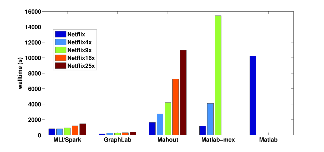
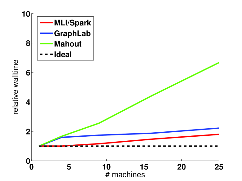
(a)	(b)	(c)

Figure 3: ALS experiments. (a) Lines of code. (b) Execution time for weak scaling. (c) Weak scaling.

IV-B Collaborative Filtering: Alternating Least Squares

Matrix factorization is a technique used in recommender systems to predict user-product associations. Let $M\in\mathbb{R}^{m\times n}$ be some underlying matrix and suppose that only a small subset, $\Omega(M)$, of its entries are revealed. The goal of matrix factorization is to find low-rank matrices $U\in\mathbb{R}^{m\times k}$ and $V\in\mathbb{R}^{n\times k}$, where $k\ll n,m$, such that $M\approx UV^{T}$. Commonly, $U$ and $V$ are estimated using the following bi-convex objective:

$$\min_{U,V}\sum_{(i,j)\in\Omega(M)}(M_{ij}-U_{i}^{T}V_{j})^{2}+\lambda(||U||_{F}^{2}+||V||_{F}^{2})\,.$$ (2)

Alternating least squares (ALS) is a widely used method for matrix factorization that solves (2) by alternating between optimizing $U$ with $V$ fixed, and $V$ with $U$ fixed, using a well-known closed-form solution at each step [27].

Experimental Setup and Data

We test both strong and weak scaling experiments using 1, 4, 9, 16, and 25 machines with the same specifications as in our previous experiments. We run our weak scaling experiments on a training set of up to approximately 50 GB of collaborative filtering data. This data is created by repeatedly tiling the Netflix collaborative filtering dataset. This allows us to maintain the sparsity structure of the dataset, and increase the number of parameters in a fixed manner. For weak scaling, the size of the dataset is proportional to the number of machines used in the cluster for the experiment. Thus, when running the largest experiment on 25 machines, we use a dataset that is 25x the size of the Netflix dataset. In our strong scaling experiments, we trained on 9x the Netflix dataset, changing only the number of machines.

For both strong and weak scaling experiments, we keep the following parameters fixed. We run ALS for 10 iterations, use a rank of 10, and set $\lambda=.01$. We do not calculate training error or testing error for timing purposes, but note that ALS methods from all systems achieved comparable error rates at the end of 10 iterations.

Implementation

We implement ALS by updating the rows of $U$ or $V$ in parallel across machines, and then broadcasting the factors to each machine after each update. We distribute both the matrix $M$ and a transposed version of this matrix across machines in order to quickly access relevant ratings. Our reference implementation makes use of several features of MLI, including support for CSR-compressed sparse representations of matrices, several linear algebra primitives, and heavy use of MLTable functionality. Linear algebra methods such as matrix transpose, matrix multiplication, and solving linear systems are supported. LocalMatrix also supports important access methods, such as the nonZeroIndices, which returns the nonzero column indices for a given row.

We compare our system to the latest versions of Mahout and GraphLab on the same cluster, and MATLAB running on a similarly configured machine. In addition, we test a version of ALS in MATLAB using mex, an interface that allows MATLAB to call directly into C++/Fortran routines. Comparing MLI to these other implementations, we see that the MLNumericTable and LocalMatrix objects provide convenient abstractions for patterns, thus resulting in concise code. Indeed, Figure A9 shows that our implementation is about the same length as the MATLAB code, while Figure 3(a) shows the stark comparison in code length in comparison to Mahout and GraphLab.

Results

In our weak scaling experiments for ALS (Figures 3b, 3c), we see that our system outperforms MATLAB and the highly-optimized MATLAB-Mex, at even moderate levels of data. Both MATLAB and MATLAB-Mex run out of memory before successfully running the 16x or 25x Netflix datasets. We remain within 4x of the highly specialized system GraphLab, and maintain a similar scaling pattern. We outperform Mahout both in terms of total execution time for each run and scaling across cluster size.

We see similarly promising results with our strong scaling experiments as illustrated in the Appendix - with MATLAB running out of memory before completing on the 9x Netflix dataset, and GraphLab outperforming MLI by less than a factor of 4x.

IV-C Configuration Considerations

Although we ran all of our experiments on comparable or identical hardware, different software systems varied drastically in terms of ease of installation, configuration, and executing code.

Vowpal Wabbit

To use VW in cluster mode, users must carefully partition their datasets into equally sized compressed files of training data, where the total number of files should equal the number of map tasks that the user desires to use concurrently on the cluster. Although VW uses Hadoop Streaming to launch cluster tasks, it eschews the traditional MapReduce paradigm in favor of AllReduce. To support this new communication primitive, it must open a side-channel TCP socket between map tasks to communicate incremental results. The combination leads to a failure-prone system as well as difficulty in data preparation.

Mahout

Mahout is fairly easy to set up on an already existing Hadoop cluster, and its input file formats are reasonably close to our own. However, in order to run Mahout effectively on problems larger than the traditional Netflix dataset, the user must take great care to tune job memory configuration parameters correctly to ensure that jobs complete in a performant manner.

GraphLab

While GraphLab performed very well in our speed and scalability tests, it was rather difficult to set up and integrate with an existing cluster with distributed data stored in HDFS. In order to set up GraphLab, users must configure their clusters with MPI, download, build and install GraphLab and its required dependencies, and manually copy the software to each machine on the cluster. If a single input matrix will not fit into memory, it must be stored and loaded as multiple separate files. This complicates preprocessing and requires developers to take extra steps depending on their problem sizes.

MLI and Spark

Setting up and configuring our system built on MLI and Spark is comparatively easy. Launching a well configured cluster required a single command, and our software ships with all its dependencies listed in SBT, and can be compiled and run on a cluster simply by setting a few environment variables and running one Scala program. New algorithms can be easily added to the system as new Scala classes, and driver programs are easily generated based on examples in the existing library.

V Conclusion

We have presented MLI, an API for building scalable distributed machine learning algorithms. We have shown that its components, MLTable and LocalMatrix, are useful primitives for data loading and transformation as well as data-local linear algebra operations. We have shown how these primitives can be used to code two fairly different but representative algorithms. We evaluated these algorithms in terms of both ease-of-development and computational performance, based on an implementation of MLI against Spark, comparing our system with several existing ones. Our results show that we can provide ML developers the tools to construct high performance distributed ML algorithms without onerous programming complexity. MLI is a foundational layer in our larger efforts with MLbase, a system designed to simplify large-scale ML.

Operation	Arguments	Returns	Semantics
project	Seq[Index]	MLTable	Select a subset of columns from a table.
union	MLTable	MLTable	Concatenate two tables with identical schemas.
filter	MLRow $\Rightarrow$ Bool	MLTable	Select a subset of rows from a data table given a functional predicate.
join	MLTable, Seq[Index]	MLTable	Inner join of two tables based on a sequence of shared columns.
map	MLRow $\Rightarrow$ MLRow	MLTable	Apply a function to each row in the table.
flatMap	MLRow $\Rightarrow$ TraversableOnce[MLRow]	MLTable	Apply a function to each row, producing 0 or more rows as output.
reduce	Seq[MLRow] $\Rightarrow$ MLRow	MLTable	Combine all rows in a table using an associative, commutative reduce function.
reduceByKey	Int, Seq[MLRow] $\Rightarrow$ MLRow	MLTable	Combine all rows in a table using an associative, commutative reduce function on a key-by-key basis where a key column is the first argument.
matrixBatchMap	LocalMatrix $\Rightarrow$ LocalMatrix	MLNumericTable	Execute a batch function on a local partition of the data. Output matrices are concatenated to form a new table.
numRows	None	Long	Returns number of rows in the table.
numCols	None	Long	Returns the number of columns in the table.

Figure A1: MLTable API Illustration. This table captures core operations of the API and is not exhaustive.

⬇

6 def main(args: Array[String]) {

7 val mc = new MLContext("local")

8

9 //Read in table from file on HDFS.

10 val rawTextTable = mc.textFile(args(0))

11

12 //Run feature extraction on the raw text - get the top 30000 bigrams.

13 val featurizedTable = tfIdf(nGrams(rawTextTable, n=2, top=30000))

14

15 //Cluster the data using K-Means.

16 val kMeansModel = KMeans(featurizedTable, k=50)

17 }

Figure A2: Loading, featurizing, and learning clusters on a corpus of Text Data.

Family	Example Uses	Returns	Semantics
Shape	dims(mat), mat.numRows, mat.numCols	Int or (Int,Int)	Matrix dimensions.
Composition	matA on matB, matA then matB	Matrix	Combine two matrices row-wise or column-wise.
Indexing	mat(0,??), mat(10,10), mat(Seq(2,4), 1)	Matrix or Scalar	Select elements or sub-matrices.
Reverse Indexing	mat(0,??).nonZeroIndices	Seq[Index]	Find indices of non-zero elements.
Updating	mat(1,2) = 5, mat(1, Seq(3,10)) = matB	None	Assign values to elements or sub-matrices.
Arithmetic	matA + matB, matA - 5, matA / matB	Matrix	Element-wise arithmetic between matrices and scalars or matrices.
Linear Algebra	matA times matB, matA dot matB, matA.transpose, matA.solve(v), matA.svd, matA.eigen, matA.rank	Matrix or Scalar	Basic and extended linear algebra support.

Figure A3: LocalMatrix API Illustration

⬇

1function w = log_reg(X, y, maxiter, learning_rate)

2 [n, d] = size(X);

3 w = zeros(d,1);

4 for iter = 1:maxiter

5 grad = X’␣*␣(sigmoid(X␣*␣w)␣-␣y);

6␣␣␣␣w␣=␣w␣-␣learning_rate␣*␣grad;

7␣␣end

8end

9

10%␣applies␣sigmoid␣function␣component-wise␣on␣the␣vector␣x

11function␣s␣=␣sigmoid(x)

12␣␣s␣=␣1␣./␣(1␣+␣exp(-1␣.*␣x));

13end

⬇

20object LogisticRegressionAlgorithm extends NumericAlgorithm[LogisticRegressionParameters] {

21

22 def defaultParameters() = LogisticRegressionParameters()

23

24 def sigmoid(z: Double): Double = 1.0/(1.0 + math.exp(-1.0*z))

25

26 def train(data: MLNumericTable, params: LogisticRegressionParameters): LogisticRegressionModel = {

27 val d = data.numCols-1

28

29 def gradient(vec: MLVector, w: MLVector): MLVector = {

30 val x = MLVector(vec.slice(1,vec.length))

31 x times (sigmoid(x dot w) - vec(0))

32 }

33

34 //Run gradient descent on the data.

35 val optParams = StochasticGradientDescentParameters(

36 wInit = MLVector.zeros(d),

37 grad = gradient,

38 learningRate = params.learningRate)

39 val weights =StochasticGradientDescent(data, optParams)

40

41 new LogisticRegressionModel(data.toMLTable, params, weights)

42 }

43}

⬇

5

6object StochasticGradientDescent extends MLOpt with Serializable {

7

8 def apply(data: MLNumericTable, params: StochasticGradientDescentParameters): MLVector = {

9 var weights = wInit

10 val n = data.numRows

11 var i = 0

12

13 //Main loop of SGD. Calls local SGD and averages parameters.

14 while(i < params.maxIter) {

15 weights = data.matrixBatchMap(localSGD(_, weights, params.learningRate, params.grad)).reduce(_ plus _) over data.partitions.length

16 i+=1

17 }

18 weights

19 }

20

21 def localSGD(data: LocalMatrix, weights: MLVector, lambda: Double, gradientFunction: (MLVector, MLVector) => MLVector): LocalMatrix = {

22 var localWeights = weights

23 for (i <- data.toMLVectors) {

24 //Compute the gradient and update the model.

25 val grad = gradientFunction(i, loc)

26 localWeights = localWeights minus (grad times lambda)

27 }

28 localWeights

29 }

30}

Figure A4: Logistic Regression Code in MATLAB (top) and MLI (middle, bottom).

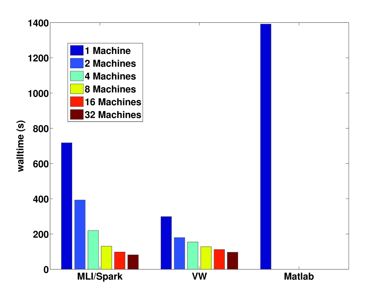
Figure A5: Execution time for strong scaling for logistic regression.

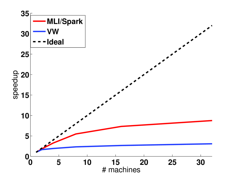
Figure A6: Strong scaling for logistic regression

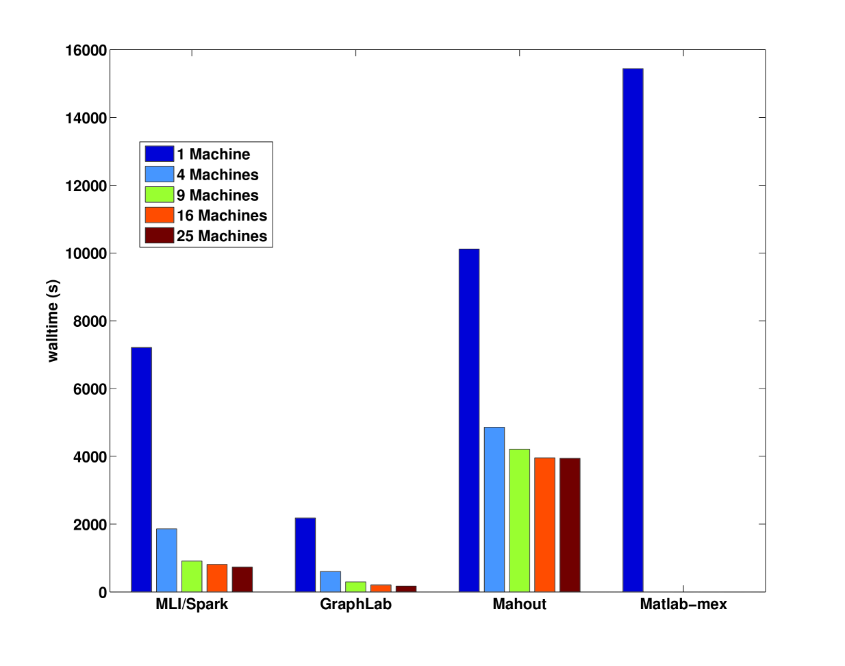
Figure A7: Execution time for strong scaling for ALS.

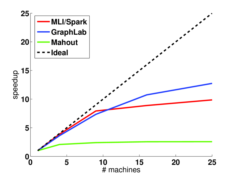
Figure A8: Strong scaling for ALS

⬇

22function [U, V] = ALS_matlab(M, U, V, k, lambda, maxiter)

23

24 % Initialize variables

25 [m,n] = size(M);

26 lambI = lambda * eye(k);

27 for q = 1:m

28 Vinds{q} = find(M(q,:) ~= 0);

29 end

30 for q=1:n

31 Uinds{q} = find(M(:,q) ~= 0);

32 end

33

34 % ALS main loop

35 for iter=1:maxiter

36 parfor q=1:m

37 Vq = V(Vinds{q},:);

38 U(q,:) = (Vq’*Vq␣+␣lambI)␣\␣(Vq’␣*␣M(q,Vinds{q})’);

39␣␣␣␣end

40␣␣␣␣parfor␣q=1:n

41␣␣␣␣␣␣Uq␣=␣U(Uinds{q},:);

42␣␣␣␣␣␣V(q,:)␣=␣(Uq’*Uq␣+␣lambI)␣\␣(Uq’␣*␣M(Uinds{q},q));

43␣␣␣␣end

44␣␣end

45end

⬇

9object BroadcastALS {

10 def train(trainData: MLTable, k: Int, lambda: Double,

11 maxIter: Int): (LocalMatrix, LocalMatrix) = {

12 val ctx = trainData.context

13 val m = trainData.numRows

14 val n = trainData.numCols

15 val trainDataTrans = trainData.transpose

16 val lambI = LocalMatrix.eye(k) * lambda

17 // Initialize U and V matrices randomly

18 val U0 = LocalMatrix.rand(m, k)

19 val V0 = LocalMatrix.rand(n, k)

20 (0 until maxIter).foldLeft((U0, V0))((UV, iterNum) => {

21 val U = UV._1

22 val V = UV._2

23 // Broadcast V

24 val V_b = ctx.broadcast(V)

25 // Update U matrix

26 val newU = computeFactor(trainData, V_b, lambI)

27 // Broadcast U

28 val U_b = ctx.broadcast(newU)

29 // Update V matrix

30 val newV = computeFactor(trainDataTrans, U_b, lambI)

31 (newU, newV)

32 })

33 }

34

35 def computeFactor(trainData: MLTable, fixedFactor: Broadcast[LocalMatrix],

36 lambI: LocalMatrix): LocalMatrix = {

37 trainData.map(localALS(_, fixedFactor.value, lambI)).toLocalMatrix

38 }

39

40 def localALS(trainDataPart: MLRow, Y: LocalMatrix, lambI: LocalMatrix) = {

41 val tuple = trainDataPart.tuple

42 val Yq = Y.getRows(tuple.nonZeroIndices)

43 val resultMat = ((Yq.transpose times Yq) + lambI).solve(Yq.transpose times tuple.nonZeroProjection)

44 resultMat.toVector

45 }

46}

Figure A9: Matrix Factorization via ALS code in MATLAB (top) and MLI (bottom).

References

- [1] “Apache mahout,” http://mahout.apache.org/.
- [2] Y. Low et al., “Graphlab: A new framework for parallel machine learning,” in UAI, 2010.
- [3] J. E. Gonzalez et al., “Powergraph: distributed graph-parallel computation on natural graphs,” in OSDI, 2012.
- [4] A. Ghoting et al., “Systemml: Declarative machine learning on mapreduce,” in ICDE, 2011, pp. 231–242.
- [5] Y. Bu et al., “Scaling datalog for machine learning on big data,” CoRR, vol. abs/1203.0160, 2012.
- [6] A. K. Sujeeth et al., “Optiml: An implicitly parallel domain-specific language for machine learning,” in ICML, 2011.
- [7] “SHOGUN,” http://shogun-toolbox.org/page/home/.
- [8] “Vowpal wabbit,” http://hunch.net/~vw/.
- [9] A. Talwalkar et al., “Mlbase: A distributed machine learning wrapper,” in NIPS Big Learning Workshop, 2012.
- [10] T. Kraska et al., “Mlbase: A distributed machine-learning system,” in CIDR, 2013.
- [11] M. Zaharia et al., “Resilient distributed datasets: A fault-tolerant abstraction for in-memory cluster computing,” in NSDI, 2012.
- [12] J. M. Hellerstein et al., “The madlib analytics library or mad skills, the sql,” in PVLDB, 2012.
- [13] A. Kumar, F. Niu, and C. Ré, “Hazy: Making it easier to build and maintain big-data analytics,” 2013.
- [14] “Weka,” http://www.cs.waikato.ac.nz/ml/weka/.
- [15] “Scikit learn,” http://scikit-learn.org.
- [16] “Google Prediction API,” https://developers.google.com/prediction/.
- [17] Venkataraman et al., “Presto: distributed machine learning and graph processing with sparse matrices,” in EuroSys, 2013.
- [18] “Matlab distributed computing server,” http://www.mathworks.com/products/distriben/.
- [19] “R for hadoop,” http://www.revolutionanalytics.com/products/r-for-hadoop.php.
- [20] R.-E. Fan et al., “Liblinear: A library for large linear classification,” JMLR, vol. 9, pp. 1871–1874, 2008.
- [21] R. R. Curtin et al., “MLPACK: A Scalable C++ Machine Learning Library,” in NIPS Big Learning Workshop, 2011.
- [22] Y. Yu et al., “DryadLINQ: A System for General-Purpose Distributed Data-Parallel Computing Using a High-Level Language.” OSDI, 2008.
- [23] V. R. Borkar et al., “Hyracks: A flexible and extensible foundation for data-intensive computing,” in ICDE, 2011.
- [24] B. Catanzaro et al., “Sejits: Getting productivity and performance with selective embedded jit specialization,” 2009.
- [25] J. Deng, W. Dong, R. Socher, L.-J. Li, K. Li, and L. Fei-Fei, “ImageNet: A Large-Scale Hierarchical Image Database,” in CVPR09, 2009.
- [26] “Cluster parallel learning. [with vowpal wabbit],” https://github.com/JohnLangford/vowpal_wabbit/wiki/Cluster_parallel.pdf.
- [27] Y. Koren et al., “Matrix factorization techniques for recommender systems,” Computer, vol. 42, no. 8, pp. 30–37, 2009.