The overlap in glassy systems

Abstract

In this paper I will consider many of the various definitions of the overlap and of its probability distribution that have been introduced in the literature starting from the original papers of Edwards and Anderson; I will present also some of the most recent results on the probability distribution of the local overlap in spin glasses. These quantities are related to the fluctuation dissipation relations both in their local and in their global versions.

1 Introduction

A fundamental step forward in the history of spin glasses is represented by the papers of Edwards and Anderson of 1975 [1]. There are many ideas in these papers that have formed the leitmotive of the research of the subsequent years: the use of the replica method, the mean field equations, the overlap order parameter. In their approximate solution of the thermodynamics of spin glasses EA introduced the almost simplest three dimensional model Hamiltonian the Edward Anderson model: it t captures the essential ingredients of quenched disorder and frustration. In spin glasses the Edward Anderson model (and its later modifications) plays the same role of the Ising model in the study of ferromagnetism: this model became a standard both for the theoretical analysis and for the numerical simulations.

In this paper I will concentrate on the definition of the overlap and it subsequent evolution. I will show how this simple and deep theoretical tool has been used in order to obtain information in quite diverse situations and how during its evolution it has acquired a multitude of facets.

In section two I will recall the original definition of the overlap, I will show how it can be extended to the case where replica symmetry is broken and many finite volume pure states are present and how the probability distribution of the overlap controls the value of the free energy in the mean field approximation.

In section three I will show how the various definitions of the overlap are related to the various definitions of the magnetic susceptibility. The magnetic susceptibility may be defined in different ways and different definitions lead different values when replica symmetry is broken, as happens in experiments.

In section four I will show how a thermodynamically stable definition of the probability distribution of the overlap is possible, i.e. how to define some functions $\tilde{P}(q)$ such that they do not fluctuate from system to system and they coincide with the ensemble average of the sample dependent probability distribution function of the overlap. Two different approaches may be used: the study of the partition function in presence of a small random magnetic field and the introduction of generalized susceptivities as the response to many spin perturbations. The generalization of this last approach leads to the introduction of the probability distribution of a site dependent overlap.

Finally in the last section before the conclusions the generalized fluctuation dissipation relations are introduced. Their relations with the overlap distribution are elucidated both for the global case and for the local case. These last relations are particularly interesting as far as they lead to the prediction that in an aging system the effective temperature is site independent.

2 The original definition of the overlap

2.1 Only one state

Let us firstly recall some of the essential ideas in the Edwards and Anderson papers. We first introduce the Edwards Anderson model: the spins are defined on a regular lattice (e.g. in three dimensions on simple cubic lattice); their interaction is only among the nearest neighbours pairs:

$$H_{J}[\sigma]=\sum_{i,k}J_{i,k}\sigma_{i}\sigma_{j}+h\sum_{i}\sigma_{i}\ ,$$ (1)

where the sum is over nearest neighbours on a lattice, the $J_{i,k}$ independently random interactions chosen from a characteristic distribution, and the $\sigma$ are classical vector spins (the simplest model, that has been the subject of most subsequent work, is the Ising analogue of the this model). This model is now universally known as the Edwards-Anderson model and is the paradigm for spin glass theory. The model is not generally soluble exactly and Edwards and Anderson used approximate mean field and variational methods in their analysis to obtain a new type of phase transition.

Edwards and Anderson chose the distribution $P(J)$ to be Gaussian centred at zero, presumably to have just a single characteristic scale (the standard deviation), to exclude any possibility of periodic order, and to take advantage of the simplicity of Gaussian integrals. In others version of the model, $J_{i,k}$ take the values $\pm 1$ with equal probability: this change in the distribution of the $J_{i,k}$ does not change the behaviour of the model at least not a too low temperature (some minor changes may be present in the low temperature limit).

The finite volume free energy is defined in the usual way:

$$F_{J}=-{\ln(Z_{J})\over\beta V}\ ,$$ (2)

$$Z_{J}=\sum_{\{\sigma\}}\exp(-\beta H_{J}[\sigma])\ .$$

In the infinite volume limit $F_{J}$ becomes $J$ independent (with probability 1) and will be denoted by $F$. The value of $F$ in the infinite volume limit can also be computed by first averaging over the $J$ (generally speaking this average will be denoted by a bar) and later sending the volume to infinity:

$$F=\lim_{V\to\infty}\overline{F_{J}}\ .$$ (3)

Now we would like to define an order parameter in the same way as in the ferromagnetic case. Also if we suppose that at low temperature there is a spontaneous magnetization $m_{i}$, it is difficult to mimic the steps that are used to define a global magnetization in the ferromagnetic case. In this case the magnetization density can be written as

$$m={\sum_{i}g_{i}m_{i}\over V}={\sum_{i}g_{i}\langle\sigma_{i}\rangle\over V}\ ,$$ (4)

where $V$ is the volume and $g_{i}$ is the ground state (i.e. the lowest energy state), that in the ferromagnetic case is given by $g_{i}=1$.

A similar definition of the order parameter in spin glasses presents two difficulties:

• Also in the case with Gaussian couplings $J$, where there is no accidental degeneracy of the ground states, it is not evident that the magnetization at finite temperature should points in the same direction of the ground state, that is the zero temperature magnetizations (this statement is likely wrong due to chaos in temperature).

• Also if the previous difficulty were not present, the computation of the ground state configuration is not a simple task and no simple formulae are available.

The proposal of Edward Anderson was to use the magnetizations themselves instead of the $g$’s. This may looks strange, but is leads to quite reasonable formulae:

$$q_{EA}={\sum_{i}m_{i}^{2}\over V}={\sum_{i}\langle\sigma_{i}\rangle^{2}\over V}\ .$$ (5)

The previous equation can also be written as

$$q_{EA}={\sum_{i}\langle\sigma_{i}\tau_{i}\rangle\over V}\ ,$$ (6)

where now we consider a system composed by two identical copies (replicas or clones) of the original system ($\sigma$ and $\tau$) with a total Hamiltonian that is equal to

$$H_{J}[\sigma,\tau]=H_{J}[\sigma]+H_{J}[\tau]\ .$$ (7)

The quantity

$$q[\sigma,\tau]={\sum_{i}\sigma_{i}\tau_{i}\over V}$$ (8)

is the overlap of the two replicas and the Edwards Anderson order parameter can be written as

$$q_{EA}=\langle q[\sigma,\tau]\rangle$$ (9)

2.2 Many states

If there are multiple states, as it is usual when there is a spontaneous magnetization, one must be careful: in the previous formulae the value of $q_{EA}$ could depend on the state where the variables $\sigma$ and $\tau$ live. In order to get an handle of what may happen in this situation, it is heuristically convenient to suppose that the finite volume Gibbs measure may be decomposed (with a good approximation) into the sum of pure finite volume states, i.e.

$$\langle\cdot\rangle=\sum_{\alpha}w_{\alpha}\langle\cdot\rangle_{\alpha}\ .$$ (10)

In this way each state may be characterized by a magnetization $m(i)_{\alpha}$ such that

$$m(i)_{G}\equiv\langle\sigma_{i}\rangle=\sum_{\alpha}w_{\alpha}\langle\sigma_{i}\rangle_{\alpha}=\sum_{\alpha}w_{\alpha}m(i)_{\alpha}\ .$$ (11)

We also define an overlap matrix

$$q_{\alpha,\gamma}={\sum_{i}m(i)_{\alpha}m(i)_{\gamma}\over V}\ .$$ (12)

In principle we could define an $\alpha$ dependent Edward Anderson parameter,

$$q_{EA}(\alpha)={\sum_{i}m(i)_{\alpha}^{2}\over V}=q_{\alpha,\alpha}\ .$$ (13)

As far as all the different states must have the same free energy density one expect that in the infinite volume limit $q_{EA}(\alpha)$ is independent from $\alpha$.

In the definition of $q_{EA}$ we must be careful to compute the magnetization in one of the pure states. If we use the Gibbs magnetization to compute the Edward Anderson parameter, we find a different result. Indeed we have that

$$q_{G}\equiv{\sum_{i}m(i)_{G}^{2}\over V}=\sum_{\alpha,\gamma}w_{\alpha}w_{\gamma}q_{\alpha,\gamma}\ .$$ (14)

For each given sample it is convenient to introduce the function $P_{J}(q)$ defined as the probability distribution of the overlap $q[\sigma,\tau]$ in the two replicas system [3, 4]. This function is well defined and it can be used as starting point of the theory without making reference to the decomposition in finite volume pure states. However if we assume that such a decomposition can be done, we find that

$$P_{J}(q)=\sum_{\alpha,\gamma}w_{\alpha}w_{\gamma}\delta(q-q_{\alpha,\gamma})\ .$$ (15)

It is interesting to note that

$$q_{G}=\int P_{J}(q)q\;dq\ .$$ (16)

In the usual case, i.e. when there is only one phase, the function $P(q)$ has only one delta function. In ferromagnetic cases at zero magnetic field, where two states exist with spontaneous magnetization, the function $P(q)$ is given by

$$P(q)=\frac{1}{2}\delta(q-m^{2})+\frac{1}{2}\delta(q+m^{2})\ .$$ (17)

In systems where there is a global symmetry that change the sign of all the spins, one has $P(q)=P(-q)$ and in order to avoid this duplication of information one usually uses a function $P(q)$ that is restricted only to positive $q$: in this case $P(q)$ takes a value that is twice the original one. If we use this prescription in the ferromagnetic case the function $P(q)$ reduces to a simple delta function. Similar prescription are used in presence of some symmetry.

In the nutshell we can characterize the phase structure of the system by giving the function $P_{J}(q)$ or the set $\Omega$ of all the $w$’s and $q$’s (i.e. $\Omega=\{w_{\alpha},q_{\alpha,\gamma}$). The two descriptions are more or less equivalent and we can easily switch between them.

In the case of spin glasses we expect that the function $P_{J}(q)$ fluctuates from sample to sample and therefore the crucial quantity to know is the probability distribution ${\cal P}[P]$ of the probability $P_{J}(q)$ [5] or equivalently the probability distribution of $\Omega$ (i.e. $\mu(\Omega)$). A crucial role is played by the average

$$P(q)=\overline{P_{J}(q)}\ .$$ (18)

When the ultrametricity condition is satisfied [3], i.e. when

$$q_{\alpha,\gamma}\geq\min(q_{\alpha,\delta},q_{\delta,\gamma})\ \ \ \forall\delta\ ,$$ (19)

if one uses the property of stochastic stability, the knowledge of the function $P(q)$ is sufficient to reconstruct the whole function $\overline{P_{J}(q)}$. In this case the different states of a given sample have a taxonomic hierarchical classification and one usually refers to this situation as the hierarchical or ultrametric approach [3].

2.3 A soluble model

In order to see if the previous construction is not empty it is convenient to consider a soluble model, where explicit computations can be done, i.e. the Sherrington Kirkpatrick model [6], that can be formally obtained as limit of the Edwards Anderson model when the dimensions of the space go to infinity. More precisely this model contains $V$ spins, the Hamiltonian has the same form as in equation (1), with the difference that the sum over $i$ and $k$ runs over all the possible pairs of different spins and the variables $J$’s have zero average and variance $V^{-1}$.

In this model is possible to prove that the function $P(q)$ cannot be a delta function, because this hypothesis leads to contradictions (i.e. negative entropy at low temperature). The real advantage of the model is its solubility, i.e. the possibility of expressing the free energy in a closed form.

If one makes the usual ultrametric hypothesis it is possible by using standard manipulations to compute the free energy as functional of the function $P(q)$. In this way one find [3]

$$F=\max_{P}F_{U}[P]\ ,$$ (20)

where $F_{U}[P]$ has a relatively simple form. In this way one can find an esplicite for the free energy [7]) that has been recently proved to be correct [8].

The ultrametricity hypothesis has never been proved rigorously. In spite of its intricacies it is essentially the simplest possible hypothesis and more complicate ansatz have never been constructed.

Quite recently it was discovered that it is possible to write a simple formula for the free energy as

$$F=\max_{\mu[\Omega]}\int d\mu[\Omega]F[\Omega]\ ,$$ (21)

where $\mu[\Omega]$ is (as before) a probability measure over the $w$’s and the $q$. This result [9] is very interesting: the esplicite form of the function $F[\Omega]$ is somewhat unusual [9] and will not reported here. A detailed computation shows that, if we consider the $\mu_{U}[\Omega]$ that correspond to the ultrametric case, we have

$$\int d\mu_{U}[\Omega]F[\Omega]=F_{U}[P]\$$ (22)

and we recover the well known result [7] that the ultrametric construction provided a lower bound to the free energy.

It is rather likely that ultrametricity is correct (although a rigorous proof is lacking) because it produces the correct value of the free energy. As far as we know that a solution of the variation problem eq.(21) is ultrametric, we have to prove that it essentially unique. It is also possible that the ultrametricity could be proved by a more direct approach [10].

3 The thermodynamic definition of the overlap

The definitions of the overlap presented in the previous sections are nice, but they rely on the decomposition into states, that for a finite volume systems is only approximate and it is very difficult to perform in practice. The fact that the overlap enters in the explicit solution of the Sherrington Kirkpatrick model hints that the overlap is a relevant quantity. It would be very important to define the overlap order parameter in a thermodynamic way.

In the ferromagnetic case this is by far the simplest approach. We add to the usual ferromagnetic interaction a constant magnetic field $\epsilon$ and we compute the $\epsilon$-dependent magnetization $m(\epsilon)$ in the infinite volume limit. Only after the infinite volume limit we send the magnetic field to zero and we find that the spontaneous magnetization $m_{s}$ is given by

$$\lim_{\epsilon\to 0^{\pm}}m(\epsilon)=\pm m_{s}\ .$$ (23)

The homologous definition for spin glasses is given as follows. We consider a system with Hamiltonian

$$H_{J}[\sigma,\tau]=H_{J}[\sigma]+H_{J}[\tau]-\epsilon Vq[\sigma,\tau]\ .$$ (24)

Let define $F(\epsilon)$ as the free energy associated to the previous Hamiltonian.

We can define the $\epsilon$-dependent overlap as the expectation of the overlap computed with this Hamiltonian. It is given by

$$q(\epsilon)=-{\partial F(\epsilon)\over\partial\epsilon}\ .$$ (25)

Exactly in the same way as in the ferromagnetic case we obtain two order parameters:

$$q_{\pm}=\lim_{\epsilon\to 0^{\pm}}q(\epsilon)\ .$$ (26)

We face now the problem of interpreting this two parameters and to give a physical meaning to the event $q_{0}\neq q_{1}$. In a first approximation for small positive $\epsilon$, the $\epsilon$ dependent part of the partition function can be written as

$$\exp(\epsilon V\beta q_{max})\ ,$$ (27)

where $q_{max}=\max_{\alpha,\gamma}q_{\alpha,\gamma}$. The maximum is reached for $\alpha=\gamma$ and in this way we identify $q_{max}$ with $q_{EA}$. We thus find that

$$q_{+}=q_{EA}\equiv q_{max}\ .$$ (28)

On the contrary for small positive $\epsilon$ the $\epsilon$ dependent part of the partition function can be written as

$$\exp(\epsilon\beta Vq_{min})\ ,$$ (29)

where $q_{min}=\min_{\alpha,\gamma}q_{\alpha,\gamma}$. In the same way we find that

$$q_{-}=q_{min}\ .$$ (30)

In presence of a non-zero magnetic field there is no accidental degeneracy present . In usual systems where the equilibrium state is unique, we would have $q_{min}=q_{max}$. On the contrary the unusual situation $q_{min}<q_{max}$ corresponds to the existence of more than one equilibrium state. In this case the expectation value of the overlap is $q_{max}$ for small positive $\epsilon$ and $q_{min}$ for small negative $\epsilon$ and it is discontinuous at $\epsilon=0$.

If we take two replicas, the value of the overlap is $q_{max}$ or $q_{min}$ in the limit of zero external fields (i.e. at $\epsilon=0$) depending if this limit is reached from a positive or a negative value; this phenomenon carries the name of replica symmetry breaking. The origine of this name is the following: if we consider a system with 4 replicas, we could apply a positive field on the overlap of the first two replicas and a negative field on the overlap of the last two replicas. In this way in the limit of zero field, in spite of the permutation symmetry among the four replicas, we find that the expectation values are not symmetric: the overlap of the first two replicas is $q_{max}$ that is different from the overlap of the other two replicas, that is just given by $q_{min}$.

It is possible to define also different overlaps that behaves in a slightly different way. The mostly studied is the so called link (or energy) overlap [11] that is defined as

$$\sum_{i,k}J_{i,k}\sigma(i)\sigma(k)J_{i,k}\tau(i)\tau(k)\ .$$ (31)

The advantage of this overlap is that it is even in the spins and it is invariant under the transformation $\sigma\to-\sigma$.

4 The two susceptibilities

Using the previous definition we can take two different replicas each in the Gibbs ensemble, at $\epsilon=0$ and compute the probability distribution of the overlap. In the most interesting case, where $q_{min}\neq q_{max}$, we are at a first order phase transition point and it is natural that intensive quantities like $q$ fluctuate. For each given instance $J$ of the system we can construct a function $P_{J}(q)$ that represent the fluctuation of this quantity.

Usually at first order transitions the fluctuations of the order parameters are not important. On the contrary here the situation is quite different. This can be seen by studying a crucial quantity like the magnetic susceptibility.

In order to simplify the analysis let us suppose that after we average on the disorder, at different points $i$ and $k$ we have that

$$\overline{\langle\sigma_{i}\sigma_{k}\rangle}=\overline{\langle\sigma_{i}\rangle\langle\sigma_{k}\rangle}=0\ .$$ (32)

This property is valid in a some model of spin glasses: e. g. in the Edwards Anderson model in the limit of zero magnetic field.

A simple computation shows that the average magnetic susceptibility is just given by

$$\chi_{eq}=\beta\int dP(q)(1-q)=\beta(1-q_{G})\ .$$ (33)

Indeed we have that

$$N\chi_{eq}=\beta\sum_{i,k=1,N}\overline{\langle\sigma_{i}\sigma_{k}\rangle-\langle\sigma_{i}\rangle\langle\sigma_{k}\rangle}\ .$$ (34)

The terms with $i\neq k$ do not contribute after the average over the systems (as consequence of eq. (32)) and the only contribution comes from the terms where $i=k$. We finally obtain

$$N\chi=\sum_{i=1,N}\overline{(1-(\langle\sigma_{i}\rangle\ )^{2}}=N\beta\left(\overline{1-\sum_{\alpha,\gamma}w_{\alpha}w_{\gamma}q_{\alpha,\gamma}}\right)\ .$$ (35)

It is interesting to note that we can also write

$$\chi=\beta(1-q_{EA})+N^{-1}\beta\sum_{\alpha,\gamma}w_{\alpha}w_{\gamma}(M_{\alpha}-M_{\gamma})^{2}$$ (36)

where $M_{\alpha}$ is the total magnetization is the state $\alpha$

$$M_{\alpha}=\sum_{i}\langle\sigma(i)\rangle_{\alpha}$$ (37)

The first term (i.e. $\chi_{LR}\equiv\beta(1-q_{EA})$) has a very simple interpretation: it is the susceptibility if we restrict the average inside one state and it is usually called the linear response susceptibility. The second term,

$$\chi_{irr}\equiv\beta\sum_{\alpha,\gamma}w_{\alpha}w_{\gamma}(q_{EA}-q_{\alpha,\gamma})\ ,$$ (38)

has a more complex physical origine: when we increase the magnetic field, the states with higher magnetization become more likely than the states with lower magnetization and this effect contributes to the increase in the magnetization. However the time to jump to a state to an other state is very high (it is strictly infinite in the infinite volume limit if non linear effects are neglected) and this effect produces the separation of time scales relevant for $\chi_{LR}$ and $\chi_{eq}$.

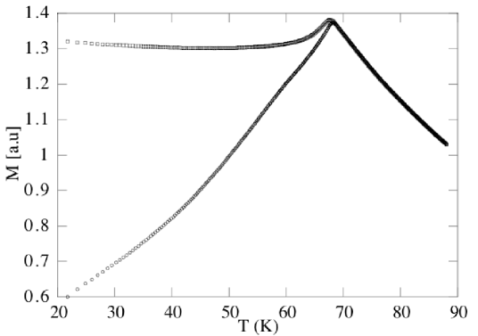
Figure 1: The experimental results for the FC (field cooled) and the ZFC (zero field cooled) magnetisation (higher and lower curve respectively) vs. temperature in a spin glass sample ($Cu_{87}Mn_{13.5}$) for a very small value of the magnetic field $H$ =1 Oe (taken from [12]). For a such a low field non linear effects can be neglected and the magnetization is proportional to the susceptibility.

If we look to real systems (e.g. spin glasses) both susceptibilities are experimentally observable.

• The first susceptibly ($\chi_{LR}$) is the susceptibly that you measure if you add an very small magnetic field at low temperature. The field should be small enough in order to neglect non-linear effects. In this situation, when we change the magnetic field, the system remains inside a given state and it is not forced to jump from a state to an other state: we measure the ZFC (zero field cooled) susceptibility, and we obtain the linear response susceptibility.

• The second susceptibility ($\chi$) can be approximately measured doing a cooling in presence of a small field: in this case the system has the ability to chose the state that is most appropriate in presence of the applied field. This susceptibility, the so called FC (field cooled) susceptibility is nearly independent from the temperature and corresponds to $\chi_{eq}$.

Therefore one can identify $\chi_{LR}$ and $\chi_{eq}$ with the ZFC susceptibility and with the FC susceptibility respectively. The experimental plot of the two susceptibilities is shown in fig. (1). They are clearly equal in the high temperature phase while they differ in the low temperature phase.

The difference among the two susceptibilities is a crucial signature of replica symmetry breaking and, if it an equilibrium phenomenon, can explained only in this framework. This phenomenon is due to the fact that a small change in the magnetic field pushes the system in a slightly metastable state, that may decay only with a very long time scale. This may happens only if there are many states that differs one from the other by a very small amount in free energy.

5 Virtual Probabilities

5.1 General considerations

The previous arguments show that the average over the different realizations $J$ of the function $P_{J}(q)$,

$$P(q)=\overline{P_{J}(q)}\ ,$$ (39)

has a deep theoretical interest. Indeed the previous formula for the equilibrium susceptibility reads as

$$\chi_{eq}=\beta(1-\int dqP(q)\;q).$$ (40)

The situation is rather strange. We have seen that we can define $q_{max}$ and $q_{min}$ in a thermodynamic way, i.e. as the response to an external field. The function $P(q)$ must be zero outside the interval $[q_{min}-q_{max}]$, however apparently the previous argument cannot be extended directly to the definition of the whole function $P(q)$. Moreover the function $P_{J}(q)$ fluctuate from sample to sample: why its average over the samples should be of some theoretical importance? If one define a function $P^{\prime}(q)$ in a different way, quite different behaviour can obtained in the infinite volume limit.

One may question why this particular definition of the function $P(q)$ is of theoretical interest. One could argue, with reasons, that only intensive quantities that are independent from the boundary conditions are physically interesting in the infinite volume limit. Order parameters should be computed by differentiating the free energy with respect the appropriate coniugate parameters. However we already know that the first moment of $P(q)$ is related to the magnetic susceptibility. It is natural to guess that by studying more complex susceptibilities one can gather enough information to reconstruct the whole function $P(q)$.

5.2 A first attempt

A first attempt to reconstruct in a thermodynamically way the function $P(q)$ can be found in [14]. We consider the Hamiltonian

$$H[\sigma]=\sum_{i,k}J_{i,k}\sigma_{i}\sigma_{j}+\sum_{i}h_{i}\sigma_{i}\ .$$ (41)

The associated partition function $Z[h]$ depends on the set of the local magnetic fields $h_{i}$. We define the generalized free energy (for positive $\epsilon$) as

$$\Phi(x,\epsilon)=-\lim_{V\to\infty}{\ln\left(\int d\mu[h]Z(\epsilon^{1/2}h)^{x})\right)\over\beta Vx}\ ,$$ (42)

where $d\mu[h]$ is a Gaussian measure: different $h$’s are independent, have zero mean and variance 1.

This definition is rather baroque: it tells us in convoluted way something on the probability distribution of the response of the system to a random magnetic field, but it has the advantage of being a bona fide thermodynamic quantity.

We can define a generalized susceptibility

$$\chi(x)={\partial\Phi(x,\epsilon)\over\partial\epsilon}|_{\epsilon=0^{+}}$$ (43)

It is easy to see that at $x=0$ $\chi(x)$ is the usual susceptibility: $\chi(0)=\chi_{eq}\ .$

It can be argued that for $0<x<1$ we have that

$${d\chi(x)\over dx}=q(x)\ ,$$ (44)

where the function $q(x)$ is defined by the condition

$$\int_{q(x)}^{1}P(q)dq=x\ .$$ (45)

Alternatively the function $q(x)$ can be computed by the condition

$${dx\over dq}=P(q)\ .$$ (46)

Although eq. (44) naturally arises in the replica formalism, its direct interpretation is not evident. By doing an explicit probabilistic computation it was shown in [14] that it is deeply related to the behaviour of the weighs $w_{\alpha}$. Here a discussion of the probabilistic derivation and/or of the probabilistic consequences of eq. (44) would be out of place. It is important to stress that the function $P(q)$, or equivalently $x(q)$ can be computed in a thermodynamic way, i.e. by differentiating the appropriate free energy.

5.3 Generalized susceptibilities

Our aim it to prove that the moments of $P(q)$ are respectively related to the static [15, 16, 17, 18] and the dynamical behaviour [19] of the system when one adds appropriate random perturbations. This approach has the advantage of being much more general; moreover it allows to define all the relevant quantities in the case of single large system (in the infinite volume limit), in the same way as in the previous section, while in the original approach the function $P(q)$ was defined as the probability distribution in an ensemble of different systems, characterized by different realizations of the disorder (i.e. $P(q)=\overline{P_{J}(q)}$). This difference is crucial if we consider the case (like glasses) where no disorder is present .

In the case of spin systems an appropriate perturbation is given by:

$$H_{p}(\sigma)=\sum_{i_{1}<\cdots<i_{p}}^{1,N}K_{i_{1},\ldots,i_{p}}\sigma_{i_{1}}\cdots\sigma_{i_{p}},$$ (47)

where the couplings $K_{i_{1},\ldots,i_{p}}$ are independent Gaussian variables with zero mean and variance $\overline{K_{i_{1},\ldots,i_{p}}^{2}}=p!/(2N^{p-1})$.

One can easily see that the canonical average of $H_{p}$ with the perturbed Hamiltonian

$$H_{\epsilon}=H_{J}+\epsilon H_{p}^{,}$$ (48)

for all values of $\epsilon$, verifies the relation

$$\overline{\langle H_{p}\rangle}=-\beta\epsilon N\left(1-\int dq\;P(q,\epsilon)\,q^{p}\right),$$ (49)

irrespectively of the specific form of $H_{J}$. Here the function $P(q,\epsilon)$ is the probability distribution of the overlap $q$ in the presence of the perturbing term in the Hamiltonian; the average is done over the new couplings $K$ at fixed $H_{J}$. The derivation, involves only an an integration by parts in a finite system.

The previous equation looks strange: the function $P_{J}(q,0)$ depends on the instance of the problem also in the infinite volume limit, while, for $\epsilon\neq 0$, $\langle H_{p}\rangle$ is a thermodynamic quantity shat cannot fluctuate in the infinite volume limit when we change the instance of the system. (at least for generic $\epsilon$). Therefore for a given large system

$$\tilde{P}_{J}(q)\neq P_{J}(q),$$ (50)

where $P_{J}(q)$ is the usual overlap probability distribution computed at $\epsilon=0$, that depends on the instance $J$, while $\tilde{P}_{J}(q)$ is the limit $\epsilon\to 0$ of the function $P_{J}(q,\epsilon)$, the function $P_{J}(q,\epsilon)$ has been computed using eq. 49 and the limit is evaluated outside the cross-over region, i.e. $\epsilon>>V^{1/2}$).

In presence of many equilibrium states, as it happens when replica symmetry is broken, the situation is rather complex. Indeed, a random perturbation reshuffles the weights of the different ergodic components in the Gibbs measure. The principle of stochastic stability [15, 16, 17, 18] assumes that, if consider an appropriate ensemble for the initial random system, we have that

$$\overline{P_{J}(q)}=\tilde{P}(q)\ .$$ (51)

There are cases where stochastic stability trivially fails, i.e. when the original Hamiltonian has an exact symmetry, that is lifted by the perturbation. The simplest case is a spin glass with a Hamiltonian invariant under spin inversion. In this case $P(q)=P(-q)$, since each pure state appears with the same weight as the spin reversed one in the unperturbed Gibbs measure. On the other hand, if we consider $H_{p}$ with odd $p$, this symmetry is lifted. This means that in the $\epsilon\to 0$ limit only half of the states are kept. If the reshuffling of their free energies is indeed random, then we shall have $\tilde{P}(q)=2\theta(q)P(q)\equiv\hat{P}(q)$. The same type of reasoning applies whenever the overlap $q$ transforms according to a representation of the symmetry group of the unperturbed Hamiltonian $H_{0}$. Once the effect of exact symmetries is taken into account, one may expect that, for a large class of systems, the limit function $\tilde{P}(q)$ in the limit of small perturbations tends to the order parameter function $\hat{P}(q)$ of the pure system where the exact symmetries are lifted.

Stochastic stability is nothing but a statement of continuity of various properties of the system at small $\epsilon$. Ordinary systems with symmetry breaking and mean-field spin glasses are examples of stochastically stable systems. In symmetry breaking systems (and in ergodic systems), the equality of $\tilde{P}$ and $\hat{P}$ is immediate, since both functions consist in a single delta function. Thus, the problem of deriving the equality between $\tilde{P}$ and $\hat{P}$, appears only when the coexisting phases are unrelated by symmetry.

Unfortunately, we are not able to characterize the class of stochastically stable systems in general. In particular, we do not know for sure whether short-range spin glass, where our theorem is most interesting, belong to this class. However, stochastic stability has been established rigorously in mean field problems [15, 16, 11].

If one studies more carefully the problems, one finds that stochastic stability has far reaching consequences, e.g.

$$\overline{P_{J}(q_{1})P_{J}(q_{2})}=\frac{2}{3}P(q_{1})P(q_{2})+\frac{1}{3}P(q_{1})\delta(q_{1}-q_{1})\ .$$ (52)

These (and other relations have been carefully numerically verified in also in numerical simulations of three dimensional spin glasses models [2].

5.4 Local overlap

Here we would like to extend the definition of the probability $P(q)$ and to define a site dependent overlap probability distribution $P_{i}(q)$, with properties that recall the global definition.

At this end let us start from a spin glass sample and let us consider $M$ identical copies of our sample: we introduce $N\times M$ $\sigma^{a}_{i}$ variables where $a=1,M$ (eventually we send $M$ to infinity) and $N$ is the (large) size of our sample ($i=1,N$). The Hamiltonian in this Gibbs ensemble is just given by

$$H_{K}(\sigma)=\sum_{a=1,M}H(\sigma^{a})+\epsilon H_{R}[\sigma]\ ,$$ (53)

where $H(\sigma^{a})$ is the Hamiltonian for a fixed choice of the couplings and the $H_{R}[\sigma]$ is a random Hamiltonian that couples the different copies of the system. A possible choice is

$$H_{R}[\sigma]=\sum_{a=1,M;i=1,N}K^{a}_{i}\sigma_{i}^{a}\sigma_{i}^{a+1}\ ,$$ (54)

where the variables $K^{a}_{i}$ are identically distributed independent random Gaussian variables with zero average and variance 1. In this way, if the original system was $d$ dimensional, the new system has $d+1$ dimensional, where the planes are randomly coupled. We can consider other ways to couple the systems (e.g. $H_{R}[\sigma]=\sum_{a,b=1,M;i=1,N}K^{a,b}_{i}\sigma_{i}^{a}\sigma_{i}^{b}$). An other possibility is

$$H_{R}[\sigma]=\sum_{a,b=1,M;i,j=1,N}K^{a,b}_{i,j}\sigma_{i}^{a}\sigma_{j}^{b}\ ,$$ (55)

where the variables $K$ are identically distributed independent random Gaussian variables with zero average and variance $(NM)^{-1}$. As we shall see later the form of $H_{R}$ is not important: its task it to weakly couple the different planes that correspond to different copies of our original system. The first choice eq. (54) is the simplest to visualize and it is the fastest for computer simulations, the last choice eq. (55) is the simplest one to analyze from the theoretical point of view. In the following we do not need to assume a particular choice.

Our central hypothesis is that all intensive self average quantities are smooth function of $\epsilon$ for small $\epsilon$. This hypothesis is a kind of generalization of stochastic stability. According to this hypothesis the dynamical local correlation functions and the response functions will go uniformly in time to the values they have at $\epsilon=0$.

We now consider in the case of non-zero $\epsilon$ two equilibrium configurations $\sigma$ and $\tau$ and let us define for given $K$ the site dependent overlap

$$q_{i}(\sigma,\tau)={\sum_{a=1,M}\sigma^{a}_{i}\tau^{a}_{i}\over M}\ .$$ (56)

We define the $K$ dependent probability distribution $P^{K}_{i}(q)$ as the probability distribution of the previous overlap. If we average over $K$ at fixed $\epsilon$ we can define

$$P^{\epsilon}_{i}(q)=\overline{P^{K}_{i}(q)}\ ,$$ (57)

where the bar denotes the average over $K$. We finally define

$$P_{i}(q)=\lim_{\epsilon\to 0}P^{\epsilon}_{i}(q)\ ,$$ (58)

where the limit $\epsilon\to 0$ is done after the limits $M\to\infty$ and $N\to\infty$ (alternatively we keep $\epsilon M$ and $\epsilon N$ much larger than 1).

Consistency with the usual approach implies that, if define

$$q_{t}={\sum_{i=1,N}q_{i}\over N}\ ,$$ (59)

the probability distribution $P_{t}(q)$ of $q_{t}$ should be self-averaging (i.e. it should be $J$ independent and it should coincide with the function $P(q)$ that is the average over $J$ of $P_{J}(q)$:

$$P_{t}(q)=P_{g}(q)\equiv\overline{P_{J}(q)}\ .$$ (60)

A detailed computation shows that this crucial relation is correct.

6 Fluctuation dissipation relations

6.1 The global Fluctuation Dissipation Relations

The usual equilibrium fluctuation theorem can be formulated as follows. If we consider a pair of conjugated variables (e.g. the magnetic field and the magnetization) the response function and the spontaneous fluctuations of the magnetization are deeply related. Indeed if $R_{eq}(t)$ is the integrated response (i.e. the variation of the magnetization at time $t$ when we add a a magnetic field from time 0 on) and $C_{eq}(t)$ is the correlation among the magnetization at time zero and at time $t$, we have that $R_{eq}(t)=\beta(C_{eq}(0)-C_{eq}(t))$, where $\beta=(kT)^{-1}$ and $3k/2$ is the Boltzmann-Drude constant $\alpha$ ($\alpha$ is the average kinetic energy of an atom at unit absolute temperature).

If we we eliminate the time and we plot parametrically $R_{eq}$ as function of $C_{eq}$ we have that

$$-{dR_{eq}\over dC_{eq}}=\beta\ .$$ (61)

The previous relation can be considered as the definition of the temperature and it is a consequence of the zeroth law of the thermodynamics.

The generalized fluctuation dissipation relations (FDR) can be formulated as follows in an aging system. Let us suppose that the system is carried from high temperature to low temperature at time 0 and it is in an aging regime. We can define a response function $R(t_{w},t)$ as the variation of the magnetization at time $t$ when we add a a magnetic field from time $t_{w}$ on; in the same way $C(t_{w},t)$ is the correlation among the magnetization at time $t_{w}$ and at time $t$. We can define a function $R_{t_{w}}(C)$ if we plot $R(t_{w},t)$ versus $C(t_{w},t)$ by eliminating the time $t$ (in the region $t>t_{w}$ where the response function is different from zero. The FDR state that for large $t_{w}$ the function $R_{t_{w}}(C)$ converge to a limiting function $R(C)$. We can define

$$-{dR\over dC}=\beta X(C)$$ (62)

where $X(C)=1$ for $C>C_{\infty}=\lim_{\to\infty}C_{eq}(t)$, and $X(C)<1$ for $C<C_{\infty}$. The shape of the function $X(C)$ give important information on the free energy landscape of the problem, as discussed at lengthy in the literature.

Using arguments that generalize the stochastic stability arguments to the dynamics [21], it can be shown the function $X(C)$ of the dynamics is related to a similar function defined in the statics. Indeed let us consider the function $x(q)$ (introduced in the previous section) defined as

$$x(q)=\int_{0}^{q}P(q^{\prime})dq^{\prime}\ .$$ (63)

Obviously $x(q)=1$ in the region where $q>q_{EA}$, where $q_{EA}$ is the maximum value of $q$ where the $P(q)$ is different from zero.

The announced relation among the dynamic FDR and the statics quantities is simple

$$X(C)=x(C)\ .$$ (64)

This basic relation can be derived using the principle of stochastic stability that assert that the thermodynamic properties of the system do not change too much if we add a random perturbation to the Hamiltonian.

6.2 The Local Fluctuation Dissipation Relations

There are recent results that indicate that the FDR relation and the static-dynamics connection can be generalized to local variables in systems where a quenched disorder is present and aging is heterogeneous. One can arrive to a local formulation of the fluctuation dissipation theorem, where local dynamical quantities are related to local overlap probability distribution.

For one given sample we can consider the local integrated response function $R_{i}(t_{w},t)$, that is the variation of the magnetization at time $t$ when we add a magnetic field at the point $i$ starting at the time $t_{w}$. In a similar way the local correlation function $C_{i}(t_{w},t)$ is defined to the correlation of among the spin at the point $i$ at different times ($t_{w}$ and $t$). Quite often in system with quenched disorder aging is very heterogenous: the function $C_{i}$ and $R_{i}$ change dramatically from on point to an other.

Local fluctuation dissipation relations (LFDT)

$$-{dR_{i}\over dC_{i}}=\beta X_{i}(C)\ ,$$ (65)

(the function $X_{i}(C)$ has quite strong variations with the site) have been derived analytically doing the appropriate approximations [22] and in simulations [23]. It has also been suggested that in spite of these strong heterogeneity, if we define the effective $\beta^{eff}_{i}$ at time $t$ at the site $i$ as ,

$$-{dR_{i}(t_{w},t)\over dC_{i}(t_{w},t)}=\beta X_{i}(t_{w},t)\equiv\beta^{eff}_{i}(t_{w},t)\ ,$$ (66)

the quantity $\beta^{eff}_{i}$ does not depend on the site. In other words a thermometer coupled to a given site would measure (at a given time) the same temperature independently on the site: different sites are thermometrically indistinguishable.

One can show that these results are general consequences of stochastic stability in an appropriate contest and that there is a local relation among static and dynamics [24]. The result is the following: we start from the local probability distribution of the overlap for a given system at point $i$ (i.e. $P_{i}(q)$), we define the function $x_{i}(q)$ as

$$x_{i}(q)=\int_{0}^{q}P_{i}(q^{\prime})dq^{\prime}\ ,$$ (67)

we show that the static-dynamic connection for local variables is very similar to the one for global variables and it is given by:

$$X_{i}(C)=x_{i}(C)$$ (68)

The property of thermometric indistinguishability of the sites turns out to be a byproduct of this approach: during an aging regime all the sites are characterized by the same effective temperature during the aging regime.

7 Conclusions

We have seen that the overlap, introduced in the original papers by Edwards and Anderson, plays a crucial role in the theory, especially if replica symmetry is spontaneously broken. The properties of the distribution probabilities of the overlap ($P(q)$) has also a fundamental role in the theory: they are the basis for a definition of the functional order parameter that enters in the computation of the free energy and of other thermodynamical relevant quantities.

The principle of stochastic stability has been introduced originally in order to explain same of the properties of the probability distribution of the overlap. It gradually became one of the most important guiding principles in the understanding of the behaviour of disordered systems.

It is possible to give two different alternative definitions of the function ($P(q)$) that are are well defined (they do not fluctuates) for a single system in the thermodynamic limit. The second definition is particularly interesting, because it is related to the dynamical behaviour of the system in off-equilibrium situations and for this reason it is directly connected to the observed experimental violations of the fluctuation dissipation theorem.

It is amazing how a very fundamental idea (the overlap between two configurations) had been so useful and appears in the theory in so many different, but related forms.

References

- [1] Edwards and Anderson, J. Phys F5 (1975) 965; J.Phys. F6,1927 (1976).
- [2] E. Marinari, G. Parisi, F. Ricci-Tersenghi, J. Ruiz-Lorenzo, F. Zuliani J.Stat. Phys. 98, 973 (2000).
- [3] M.Mézard, G.Parisi and M.A.Virasoro, Spin glass theory and beyond, World Scientific (Singapore 1987).
- [4] G.Parisi, Field Theory, Disorder and Simulations, World Scientific, (Singapore 1992).
- [5] G. Parisi, Physica Scripta, 35, 123 (1987).
- [6] D.Sherrington and S.Kirkpatrick, Phys. Rev. Lett., 35, 1792, (1975).
- [7] F.Guerra, Comm. Math. Phys. 233, 1 (2003).
- [8] M. Talagrand, C.R.A.S. 337, 111 (2003).
- [9] M. Aizenman, R. Sims, S. L. Starr An Extended Variational Principle for the SK Spin-Glass Model cond-mat/0306386.
- [10] S. Franz, G. Parisi and M. Virasoro, EuroPhys. Lett. 17, 5 (1992).
- [11] See for example E. Marinari, G. Parisi and J.J. Ruiz-Lorenzo cond-mat/0202500 or P. Contucci Replica equivalence in the Edwards-Anderson model cond-mat/0302500 and references therein.
- [12] C. Djurberg, K. Jonason and P. Nordblad, Magnetic Relaxation Phenomena in a CuMn Spin Glass, cond-mat/9810314.
- [13] D. Ruelle, Commun. Math. Phys. 48, 351 (1988).
- [14] G. Parisi, M. Virasoro J. de Physique I, 50, 3317 (1989)
- [15] F. Guerra, Int. J. Phys. B, 10, 1675 (1997).
- [16] M. Aizenman and P. Contucci, J. Stat. Phys. 92 (1998) 765.
- [17] S. Ghirlanda and F. Guerra, J. Phys. A: Math. Gen. 31 9149 (1998).
- [18] G. Parisi, On the probabilistic formulation of the replica approach to spin glasses, cond-mat/9801081.
- [19] L.F. Cugliandolo and J. Kurchan, Phys. Rev. Lett. 71, 173 (1993); J. Phys. A: Math. Gen. 27, 5749 (1994).
- [20] S. Franz and M. Mézard, Europhys. Lett. 26, 209 (1994).
- [21] S. Franz, M. Mézard, G. Parisi and L. Peliti, Phys. Rev. Lett. 81 1758 (1998).
- [22] E. Castillo, C. Chamon, L. Cugliandolo and M. Kennett, Phys. Rev. Lett. 88, 237201 (2002), Phys.Rev. Lett. 89, 217201 (2002); H.E. Castillo, C. Chamon, L. Cugliandolo, J. L. Iguain and M. Kennett, Spatially heterogeneous ages in glassy dynamics, cond-mat/0211558, cond-mat/0305044.
- [23] A. Montanari and F. Ricci-Tersenghi, A microscopic description of the aging dynamics: fluctuation-dissipation relations, effective temperature and heterogeneities, cond-mat 0207416, Aging dynamics of heterogeneous spin models, cond-mat/0305044.
- [24] G. Parisi, J. Phys. A 36 10773 (2003); Europhys. Lett. 65, 103 (2004).