A brief introduction to modern amplitude methods

Abstract:

I provide a basic introduction to modern helicity amplitude methods, including color organization, the spinor helicity formalism, and factorization properties. I also describe the BCFW (on-shell) recursion relation at tree level, and explain how similar ideas — unitarity and on-shell methods — work at the loop level. These notes are based on lectures delivered at the 2012 CERN Summer School and at TASI 2013.

1 Introduction

Scattering amplitudes are at the heart of high energy physics. They lie at the intersection between quantum field theory and collider experiments. Currently we are in the hadron collider era, which began at the Tevatron and has now moved to the Large Hadron Collider (LHC). Hadron colliders are broadband machines capable of great discoveries, such as the Higgs boson [1], but there are also huge Standard Model backgrounds to many potential signals. If we are to discover new physics (besides the Higgs boson) at the LHC, we will need to understand the old physics of the Standard Model at an exquisitely precise level. QCD dominates collisions at the LHC, and the largest theoretical uncertainties for most processes are due to our limited knowledge of higher order terms in perturbative QCD.

Many theorists have been working to improve this situation. Some have been computing the next-to-leading order (NLO) QCD corrections to complex collider processes that were previously only known at leading order (LO). LO uncertainties are often of order one, while NLO uncertainties can be in the 10–20% range, depending on the process. Others have been computing the next-to-next-to-leading order (NNLO) corrections to benchmark processes that are only known at NLO; most NNLO predictions have uncertainties in the range of 1–5%, allowing precise experimental measurements to be interpreted with similar theoretical precision. Higher-order computations have a number of technical ingredients, but they all require loop amplitudes, one-loop for NLO, and both one- and two-loop for NNLO, as well as tree amplitudes of higher multiplicity.

The usual textbook methods for computing an unpolarized cross section involve squaring the scattering amplitude at the beginning, then summing analytically over the spins of external states, and transforming the result into an expression that only involves momentum invariants (Mandelstam variables) and masses. For complex processes, this approach is usually infeasible. If there are $N$ Feynman diagrams for an amplitude, then there are $N^{2}$ terms in the square of the amplitude. It is much better to calculate the $N$ terms in the amplitude, as a complex number, and then compute the cross section by squaring that number. This approach of directly computing the amplitude benefits greatly from the fact that many amplitudes are much simpler than one might expect from the number of Feynman diagrams contributing to them.

In order to compute the amplitude directly, one has to pick a basis for the polarization states of the external particles. At collider energies, most of these particles are effectively massless: the light quarks and gluons, photons, and the charged leptons and neutrinos (decay products of $W$ and $Z$ bosons). Massless fermions have the property that their chirality and helicity coincide, and their chirality is preserved by the gauge interactions. Therefore the helicity basis is clearly an optimal one for massless fermions, because many matrix elements (the helicity-flip ones) will always vanish.

Around three decades ago, it was realized that the helicity basis was extremely useful for massless vector bosons as well [2]. Many tree-level amplitudes were found to vanish in this basis as well (which could be explained by a secret supersymmetry obeyed by tree amplitudes [3, 4]). Also, the nonvanishing amplitudes were found to possess a hierarchy of simplicity, depending on how much they violated helicity “conservation”. For example, a simple one-term expression for the tree amplitudes for scattering an arbitrary number of gluons with maximal helicity violation (MHV) was found by Parke and Taylor in 1986 [5], and proven recursively by Berends and Giele shortly thereafter [6].

As the first loop computations were performed for gluon scattering in the helicity basis [7, 8], it became apparent that (relative) simplicity of amplitudes could extend to the loop level. One way to maintain the simplicity is to use unitarity [9] to determine loop amplitudes by using tree amplitudes as input. These methods have been refined enormously over the years, and automated in order to handle very complicated processes. They now form an important part of the arsenal for theorists providing NLO results for LHC experiments. Many of the methods are now being further refined and extended to the two-loop level, and within a few years we may see a similar NNLO arsenal come to full fruition.

Besides QCD, unitarity-based methods have also found widespread application to scattering amplitudes for more formal theories, such as ${\cal N}=4$ super-Yang-Mills theory and ${\cal N}=8$ supergravity, just to mention a couple of examples. The more supersymmetry, the greater the simplicity of the amplitudes, allowing analytical results to be obtained for many multi-loop amplitudes (at least before integrating over the loop momentum). These results have helped to expose new symmetries, which have in turn led to other powerful methods for computing in these special theories.

The purpose of these lecture notes is to provide a brief and basic introduction to modern amplitude methods. They are intended for someone who has taken a first course in quantum field theory, but who has never studied these methods before. For someone who wants to go on further and perform research using such methods in either QCD or more formal areas, these notes will be far from sufficient. Fortunately, there are much more thorough reviews available. In particular, methods for one-loop QCD amplitudes have been reviewed in refs. [10, 11, 12, 13]. Also, a very recent and comprehensive article [14] covers much of the material covered here, plus a great deal more, particularly in the direction of methods for multi-loop amplitudes in more formal theories. There are also reviews of basic tree-level organization and properties [15, 16, 17] and of one-loop unitarity [18]. Other reviews emphasize ${\cal N}=4$ super-Yang-Mills theory [19, 20].

These notes are organized as follows. In section 2 we describe trace-based color decompositions for QCD amplitudes. In section 3 we review the spinor helicity formalism, and apply it to the computation of some simple four- and five-point tree amplitudes. In section 4 we use these results to illustrate the universal soft and collinear factorization of gauge theory amplitudes. We also introduce the Parke-Taylor amplitudes, and discuss the utility of spinor variables for describing collinear limits and massless three-point kinematics. In section 5 we explain the BCFW (on-shell) recursion relation for tree amplitudes, and apply it to the Parke-Taylor amplitudes, as well as to a next-to-MHV example. Section 6 discusses the application of generalized unitarity to one-loop amplitudes, and in section 7 we conclude.

2 Color decompositions

In this section we explain how to organize the color degrees of freedom in QCD amplitudes, in order to separate out pieces that have simpler analytic properties. Those pieces have various names in the literature, such as color-ordered amplitudes, dual amplitudes, primitive amplitudes and partial amplitudes. (There is a distinction between primitive amplitudes and partial amplitudes at the loop level, but not at tree level, at least not unless there are multiple fermion lines.)

The basic idea [21, 22, 15, 16] is to reorganize the color degrees of freedom of QCD, in order to eliminate the Lie algebra structure constants $f^{abc}$ found in the Feynman rules, in favor of the generator matrices $T^{a}$ in the fundamental representation of $SU(N_{c})$. Although the gauge group of QCD is $SU(3)$, it requires no extra effort to generalize it to $SU(N_{c})$, and one can often gain insight by making the dependence on $N_{c}$ explicit. Sometimes it is also advantageous (especially computationally) to consider the limit of a large number of colors, $N_{c}\rightarrow\infty$.

Gluons in an $SU(N_{c})$ gauge theory carry an adjoint color index $a=1,2,\ldots,N_{c}^{2}-1$, while quarks and antiquarks carry an $N_{c}$ or $\overline{N}_{c}$ index, $i,{\bar{\jmath}}=1,2,\ldots,N_{c}$. The generators of $SU(N_{c})$ in the fundamental representation are traceless hermitian $N_{c}\times N_{c}$ matrices, $(T^{a})_{i}^{~{}{\bar{\jmath}}}$. For computing color-ordered helicity amplitudes, it’s conventional to normalize them according to $\mathop{\rm Tr}\nolimits(T^{a}T^{b})=\delta^{ab}$ in order to avoid a proliferation of $\sqrt{2}$’s in the amplitudes.

Each Feynman diagram in QCD contains a factor of $(T^{a})_{i}^{~{}{\bar{\jmath}}}$ for each gluon-quark-anti-quark vertex, a group theory structure constant $f^{abc}$ for each pure gluon three-point vertex, and contracted pairs of structure constants $f^{abe}f^{cde}$ for each pure gluon four-vertex. The structure constants are defined by the commutator

$$[T^{a},T^{b}]\ =\ i\sqrt{2}\,f^{abc}\,T^{c}\,.$$ (1)

The internal gluon and quark propagators contract indices together with factors of $\delta_{ab}$, $\delta^{~{}{\bar{\jmath}}}_{i}$. We want to identify all possible color factors for the diagrams, and sort the contributions into gauge-invariant subsets with simpler analytic properties than the full amplitude.

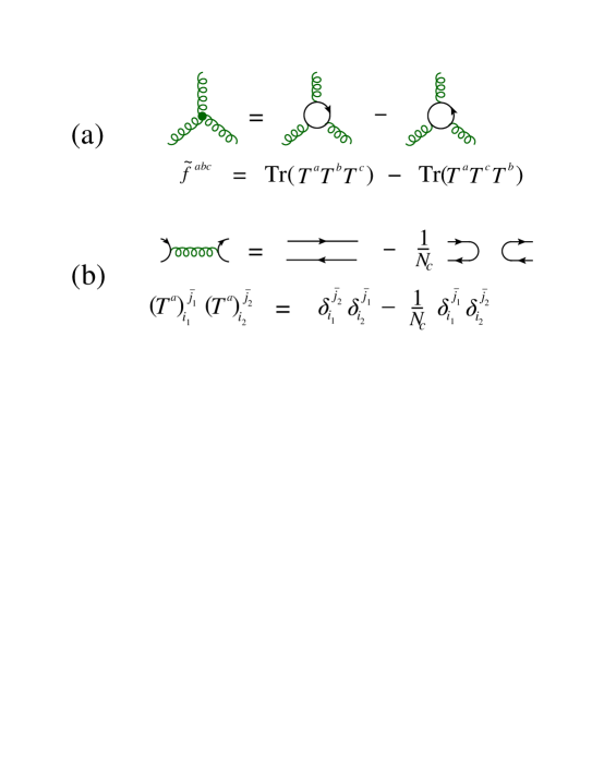
Figure 1: Graphical representation of (a) the identity for eliminating structure constants $f^{abc}$ and (b) the $SU(N_{c})$ Fierz identity for simplifying the resulting traces.

To do this, we first eliminate all the structure constants $f^{abc}$ in favor of the generators $T^{a}$, using

$$\tilde{f}^{abc}\ \equiv\ i\sqrt{2}f^{abc}\ =\ \mathop{\rm Tr}\nolimits\bigl{(}T^{a}T^{b}T^{c}\bigr{)}-\mathop{\rm Tr}\nolimits\bigl{(}T^{a}T^{c}T^{b}\bigr{)},$$ (2)

which follows from the definition (1) of the structure constants. This identity is represented graphically in fig. 1(a), in which curly lines are in the adjoint representation and lines with arrows are in the fundamental representation. After this step, every color factor for a multi-gluon amplitude is a product of some number of traces. Many traces share $T^{a}$’s with contracted indices, of the form $\mathop{\rm Tr}\nolimits\bigl{(}\ldots T^{a}\ldots\bigr{)}\,\mathop{\rm Tr}\nolimits\bigl{(}\ldots T^{a}\ldots\bigr{)}\,\ldots\,\mathop{\rm Tr}\nolimits\bigl{(}\ldots)$. If external quarks are present, then in addition to the traces there will be some strings of $T^{a}$’s terminated by fundamental indices, of the form $(T^{a_{1}}\ldots T^{a_{m}})_{i_{2}}^{~{}{\bar{\imath}}_{1}}$. In order to reduce the number of traces and strings we can apply the $SU(N_{c})$ Fierz identity,

$$(T^{a})_{i_{1}}^{~{}{\bar{\jmath}}_{1}}\,(T^{a})_{i_{2}}^{~{}{\bar{\jmath}}_{2}}\ =\ \delta_{i_{1}}^{~{}{\bar{\jmath}}_{2}}\delta_{i_{2}}^{~{}{\bar{\jmath}}_{1}}-{1\over N_{c}}\,\delta_{i_{1}}^{~{}{\bar{\jmath}}_{1}}\delta_{i_{2}}^{~{}{\bar{\jmath}}_{2}}\,,$$ (3)

where the sum over $a$ is implicit. This identity is illustrated graphically in fig. 1(b).

Equation (3) is just the statement that the $SU(N_{c})$ generators $T^{a}$ form the complete set of traceless hermitian $N_{c}\times N_{c}$ matrices. The $-1/N_{c}$ term implements the tracelessness condition. (To see this, contract both sides of eq. (3) with $\delta^{~{}i_{1}}_{{\bar{\jmath}}_{1}}$.) It is often convenient to consider also $U(N_{c})\ =\ SU(N_{c})\times U(1)$ gauge theory. The additional $U(1)$ generator is proportional to the identity matrix,

$$(T^{a_{U(1)}})_{i}^{~{}{\bar{\jmath}}}\ =\ {1\over\sqrt{N_{c}}}\ \delta_{i}^{~{}{\bar{\jmath}}}\ ;$$ (4)

when this generator is included in the sum over $a$ in eq. (3), the corresponding $U(N_{c})$ result is eq. (3) without the $-1/N_{c}$ term. The auxiliary $U(1)$ gauge field is often referred to as a photon. It is colorless, commuting with $SU(N_{c})$, with vanishing structure constants $f^{a_{U(1)}bc}=0$ for all $b,c$. Therefore it does not couple directly to gluons, although quarks carry charge under it. Real photon amplitudes can be obtained using this generator, after replacing factors of the strong coupling $g$ with the QED coupling $\sqrt{2}e$.

The color algebra can easily be carried out graphically [23], as illustrated in fig. 2. Starting with any given Feynman diagram, one interprets it as just the color factor for the full diagram, after expanding the four-gluon vertices into two three-gluon vertices. Then one makes the two substitutions, eqs. (2) and (3), which are represented diagrammatically in fig. 1. In fig. 2 we use these steps to simplify a sample diagram for five-gluon scattering at tree level. Inserting the rule fig. 1(a) in the three vertices leads to $2^{3}=8$ terms, of which two are shown in the first line. The $SU(N_{c})$ Fierz identity takes the traces of products of three $T^{a}$’s, and systematically combines them into a single trace, $\mathop{\rm Tr}\nolimits\bigl{(}T^{a_{1}}T^{a_{2}}T^{a_{3}}T^{a_{4}}T^{a_{5}}\bigr{)}$, plus all possible permutations, as shown in the second line of the figure. Notice that the $-1/N_{c}$ term in eq. (3) and fig. 1(b) does not contribute here, because the photon does not couple to gluons; that is, $f^{abI}=0$ when $I$ is the $U(1)$ generator. (The $-1/N_{c}$ term only has to be retained when a gluon can couple to a fermion line at both ends.)

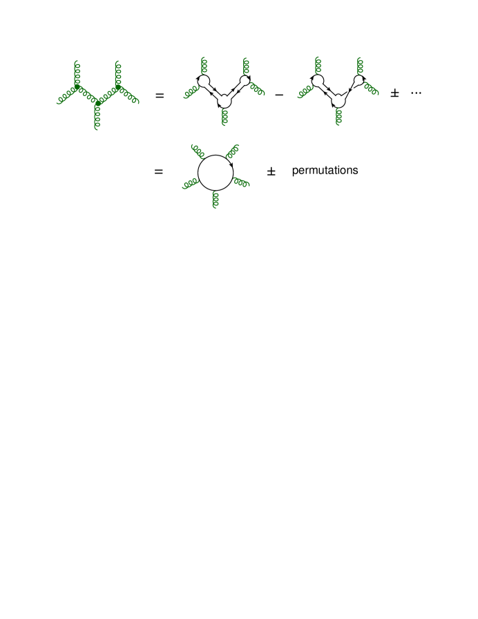
Figure 2: Graphical illustration of reducing the color factor for a five-gluon Feynman diagram to a single color trace.

From fig. 2 it is clear that any tree diagram for $n$-gluon scattering can be reduced to a sum of “single trace” terms, in which the generators $T^{a_{i}}$ corresponding to the external gluons have different cyclic orderings. The color decomposition of the the $n$-gluon tree amplitude [21] is,

$${\cal A}^{\rm tree}_{n}(\{k_{i},\lambda_{i},a_{i}\})\ =\ g^{n-2}\hskip-3.69885pt\sum_{\sigma\in S_{n}/Z_{n}}\hskip-3.69885pt\mathop{\rm Tr}\nolimits(T^{a_{\sigma(1)}}\ldots T^{a_{\sigma(n)}})\ A_{n}^{\rm tree}(\sigma(1^{\lambda_{1}}),\ldots,\sigma(n^{\lambda_{n}})).$$ (5)

Here $g$ is the gauge coupling ($g^{2}/(4\pi)=\alpha_{s}$), $k_{i},\lambda_{i}$ are the gluon momenta and helicities, and $A_{n}^{\rm tree}(1^{\lambda_{1}},\ldots,n^{\lambda_{n}})$ are the partial amplitudes, which contain all the kinematic information. $S_{n}$ is the set of all permutations of $n$ objects, while $Z_{n}$ is the subset of cyclic permutations, which preserves the trace; one sums over the set $S_{n}/Z_{n}$ in order to sweep out all cyclically-inequivalent orderings in the trace. We write the helicity label for each particle, $\lambda_{i}=\pm$, as a superscript.

The real work is in calculating the independent partial amplitudes $A_{n}^{\rm tree}$. However, they are simpler than the full amplitude because they are color-ordered: they only receive contributions from diagrams with a particular cyclic ordering of the gluons. This feature reduces the number of singularities they can contain. Tree amplitudes contain factorization poles, when a single intermediate state goes on its mass shell in the middle of the diagram. The momentum of the intermediate state is the sum of a number of the external momenta. In the color-ordered partial amplitudes, those momenta must be cyclically adjacent in order to produce a pole. For example, the five-point partial amplitudes $A_{5}^{\rm tree}(1^{\lambda_{1}},2^{\lambda_{2}},3^{\lambda_{3}},4^{\lambda_{4}},5^{\lambda_{5}})$ can only have poles in $s_{12}$, $s_{23}$, $s_{34}$, $s_{45}$, and $s_{51}$, and not in $s_{13}$, $s_{24}$, $s_{35}$, $s_{41}$, or $s_{52}$, where $s_{ij}\equiv(k_{i}+k_{j})^{2}$. Similarly, at the loop level, only the channels made out of sums of cyclically adjacent momenta will have unitarity cuts (as well as factorization poles). The number of cyclically-adjacent momentum channels grows much more slowly than the total number of channels, as the number of legs increases. Later we will use factorization properties to construct tree amplitudes, so defining partial amplitudes with a minimal number of factorization channels will simplify the construction.

Although we have mainly considered the pure-gluon case, color decompositions can be found for generic QCD amplitudes. Another simple case is the set of tree amplitudes ${\bar{q}}qgg\ldots g$ with two external quarks, which can be reduced to single strings of $T^{a}$ matrices,

$${\cal A}^{\rm tree}_{n}\ =\ g^{n-2}\sum_{\sigma\in S_{n-2}}(T^{a_{\sigma(3)}}\ldots T^{a_{\sigma(n)}})_{i_{2}}^{~{}{\bar{\jmath}}_{1}}A_{n}^{\rm tree}(1_{\bar{q}}^{\lambda_{1}},2_{q}^{\lambda_{2}},\sigma(3^{\lambda_{3}}),\ldots,\sigma(n^{\lambda_{n}})),$$ (6)

where numbers without subscripts refer to gluons. Color decompositions for tree amplitudes with more than two external quarks can be found in ref. [15].

The same ideas also work at the loop level [24]. For example, at one loop, the same graphical analysis leads to a color decomposition for pure-gluon amplitudes which contains two types of terms:

• single-trace terms, of the form $N_{c}\,\mathop{\rm Tr}\nolimits(T^{a_{1}}\ldots T^{a_{n}})$ plus permutations, which contain an extra factor of $N_{c}$ and dominate for large $N_{c}$, and

• double-trace terms, of the form $\mathop{\rm Tr}\nolimits(T^{a_{1}}\ldots T^{a_{m}})\mathop{\rm Tr}\nolimits(T^{a_{m+1}}\ldots T^{a_{n}})$ plus permutations, whose contribution to the color-summed cross section is suppressed by at least a factor of $1/N_{c}^{2}$ with respect to the leading-color terms.

Quark loops lead to contributions of the first type, but with an over all factor of the number of light quark flavors, $n_{f}$, replacing the factor of $N_{c}$.

After we have computed all of the partial amplitudes, the parton model requires us to construct the squared amplitude, averaged over the colors of the initial-state partons, and summed over the final-state colors. Using the above color decompositions, and applying Fierz identities again, this color-summed cross section can be expressed in terms of the partial amplitudes. The color factors that appear can be computed graphically. Take a single trace structure of the type shown in fig. 2, and glue the $n$ gluon lines to a second trace structure from the conjugate amplitude, which may have a relative permutation. Then apply the Fierz identity in fig. 1(b) to remove the gluon lines and reduce the resulting “vacuum” color graph to powers of $N_{c}$. (A closed loop for an arrowed line gives a factor of $\mathop{\rm Tr}\nolimits(1)=N_{c}$.)

In this way you can show that the color-summed cross section for $n$-gluon scattering,

$$d\sigma^{\rm tree}\ \propto\ \sum_{a_{i}=1}^{N_{c}^{2}-1}|{\cal A}^{\rm tree}_{n}(\{k_{i},a_{i}\})|^{2}\,,$$ (7)

takes the form,

$$d\sigma^{\rm tree}\ \propto\ N_{c}^{n}\bigg{\{}\sum_{\sigma\in S_{n}/Z_{n}}\Bigl{|}A_{n}^{\rm tree}(\sigma(1),\sigma(2),\ldots,\sigma(n))\Bigr{|}^{2}+{\cal O}(1/N_{c}^{2})\biggr{\}}\,.$$ (8)

In other words, the leading-color contributions come from gluing together two trace structures with no relative permutation, which gives rise to a planar vacuum color graph. Any relative permutation leads to a nonplanar graph, and its evaluation results in at least two fewer powers of $N_{c}$. Of course these subleading-color terms can be worked out straightforwardly as well. Another way of stating eq. (8) is that, up to $1/N_{c}^{2}$-suppressed terms, the differential cross section can be written as a sum of positive terms, each of which has a definite color flow. This description is important for the development of parton showers, which exploit the pattern of radiating additional soft gluons from these color-ordered pieces of the cross section.

3 The spinor helicity formalism

3.1 Spinor variables

Now we turn from color to spin. That is, we ask how to organize the spin quantum numbers of the external states in order to simplify the calculation. The answer is that the helicity basis is a very convenient one for most purposes. In high-energy collider processes, almost all fermions are ultra-relativistic, behaving as if they were massless. Massless fermions that interact through gauge interactions have a conserved helicity, which we can exploit by computing in the helicity basis. Although vector particles like photons and gluons do not have a conserved helicity, it turns out that the most helicity-violating processes one can imagine are zero at tree level (due to a hidden supersymmetry that relates boson and fermion amplitudes). Also, the nonzero amplitudes are ordered in complexity by how much helicity violation they have; we will see that the so-called maximally helicity violating (MHV) amplitudes are the simplest, the next-to-MHV are the next simplest, and so on.

A related question is, what are the right kinematic variables for scattering amplitudes? It is traditional to use the four-momenta, $k_{i}^{\mu}$, and especially their Lorentz-invariant products, $s_{ij}=(k_{i}+k_{j})^{2}$, as the basic kinematic variables. However, all the particles in the Standard Model — except the Higgs boson — have spin, and for particles with spin, there is a better choice of variables. Just as we rewrote the color factors for $SU(N_{c})$ adjoint states ($f^{abc}$) in terms of those associated with the smaller fundamental representation of $SU(N_{c})$ ($T^{a}$), we should now consider trading the Lorentz vectors $k_{i}^{\mu}$ for kinematic quantities that transform under a smaller representation of the Lorentz group.

The only available smaller representation of the Lorentz group is the spinor representation, which for massless vectors can be two-dimensional (Weyl spinors). So we trade the four-momentum $k_{i}^{\mu}$ for a pair of spinors,

$$k_{i}^{\mu}\quad\qquad\Rightarrow\quad\qquad u_{+}(k_{i})\equiv|i^{+}\rangle\equiv\lambda_{i}^{\alpha}\,,\qquad u_{-}(k_{i})\equiv|i^{-}\rangle\equiv\lambda_{i}^{\dot{\alpha}}\,.$$ (9)

Here $u_{+}(k_{i})=\textstyle{1\over 2}(1+\gamma_{5})u(k_{i})$ is a right-handed spinor written in four-component Dirac notation, and $\lambda_{i}^{\alpha}$ is its two-component version, $\alpha=1,2$. Similarly, $u_{-}(k_{i})=\textstyle{1\over 2}(1-\gamma_{5})u(k_{i})$ is a left-handed spinor in Dirac notation, and $\tilde{\lambda}_{i}^{\alpha}$ is the two-component version, $\dot{\alpha}=1,2$. We also give the “ket” notation that is often used. The massless Dirac equation is satisfied by these spinors,

$$\not{\hbox{\kern-2.3pt$k$}}_{i}u_{\pm}(k_{i})\ =\ \not{\hbox{\kern-2.3pt$k$}}_{i}|i^{\pm}\rangle\ =\ 0.$$ (10)

There are also negative-energy solutions $v_{\pm}(k_{i})$, but for $k_{i}^{2}=0$ they are not distinct from $u_{\mp}(k_{i})$. The undotted and dotted spinor indices correspond to two different spinor representations of the Lorentz group.

We would like to build some Lorentz-invariant quantities out of the spinors, which we can do using the antisymmetric tensors $\varepsilon^{\alpha\beta}$ and $\varepsilon^{\dot{\alpha}\dot{\beta}}$. We define the spinor products,

$$\left\langle i\,j\right\rangle\ \equiv \ \varepsilon^{\alpha\beta}(\lambda_{i})_{\alpha}(\lambda_{j})_{\beta}\ =\ \bar{u}_{-}(k_{i})u_{+}(k_{j}),$$ (11)

$$\left[i\,j\right]\ \equiv \ \varepsilon^{\dot{\alpha}\dot{\beta}}(\tilde{\lambda}_{i})_{\dot{\alpha}}(\lambda_{j})_{\dot{\beta}}\ =\ \bar{u}_{+}(k_{i})u_{-}(k_{j}),$$ (12)

where we give both the two- and four-component versions.

Recall the form of the positive energy projector for $m=0$:

$$u_{+}(k_{i})\bar{u}_{+}(k_{i})\ =\ |i^{+}\rangle\,\langle i^{+}|\ =\ \textstyle{1\over 2}(1+\gamma_{5})\not{\hbox{\kern-2.3pt$k$}}_{i}\,\textstyle{1\over 2}(1-\gamma_{5}).$$ (13)

In two-component notation, this relation becomes, using the explicit form of the Pauli matrices,

$$(\lambda_{i})_{\alpha}(\tilde{\lambda}_{i})_{\dot{\alpha}}\ =\ k_{i}^{\mu}(\sigma_{\mu})_{\alpha\dot{\alpha}}\ =\ (\not{\hbox{\kern-2.3pt$k$}}_{i})_{\alpha\dot{\alpha}}\ =\ \left(\begin{matrix}k_{i}^{t}+k_{i}^{z}&k_{i}^{x}-ik_{i}^{y}\\ k_{i}^{x}+ik_{i}^{y}&k_{i}^{t}-k_{i}^{z}\\ \end{matrix}\right).$$ (14)

Note that the determinant of this $2\times 2$ matrix vanishes, $\det(\not{\hbox{\kern-2.3pt$k$}}_{i})=k_{i}^{2}=0$, which is consistent with its factorization into a column vector $(\lambda_{i})_{\alpha}$ times a row vector $(\tilde{\lambda}_{i})_{\dot{\alpha}}$.

Also note that if the momentum vector $k_{i}^{\mu}$ is real, then complex conjugation is equivalent to transposing the matrix $\not{\hbox{\kern-2.3pt$k$}}_{i}$, which via eq. (14) corresponds to exchanging the left- and right-handed spinors, $(\tilde{\lambda}_{i})_{\dot{\alpha}}\leftrightarrow(\lambda_{i})_{\alpha}$. In other words, for real momenta, a chirality flip of all spinors (which could be induced by a parity transformation) is the same as complex conjugating the spinor products,

$$\left[i\,j\right]\ =\ \left\langle i\,j\right\rangle^{\ast}\,.$$ (15)

If we contract eq. (14) with $(\sigma^{\nu})^{\dot{\alpha}\alpha}$, we find that we can reconstruct the four-momenta $k_{i}^{\mu}$ from the spinors,

$$\langle i^{+}|\gamma^{\mu}|i^{+}\rangle\ \equiv\ (\tilde{\lambda}_{i})_{\dot{\alpha}}(\sigma^{\mu})^{\dot{\alpha}\alpha}(\lambda_{i})_{\alpha}\ =\ 2k_{i}^{\mu}\,.$$ (16)

Using the Fierz identity for Pauli matrices,

$$(\sigma^{\mu})_{\alpha\dot{\alpha}}(\sigma_{\mu})^{\dot{\beta}\beta}\ =\ 2\delta_{\alpha}^{\beta}\delta_{\dot{\alpha}}^{\dot{\beta}}\,,$$ (17)

we can similarly reconstruct the momentum invariants from the spinor products,

$$2k_{i}\cdot k_{j}\,=\,\frac{1}{2}(\tilde{\lambda}_{i})_{\dot{\alpha}}(\sigma^{\mu})^{\dot{\alpha}\alpha}(\lambda_{i})_{\alpha}(\tilde{\lambda}_{j})_{\dot{\beta}}(\sigma_{\mu})^{\dot{\beta}\beta}(\lambda_{j})_{\beta}\,=\,(\lambda_{i})_{\alpha}(\lambda_{j})^{\alpha}(\tilde{\lambda}_{j})_{\dot{\alpha}}(\tilde{\lambda}_{i})^{\dot{\alpha}}\,,$$ (18)

or

$$s_{ij}\ =\ \left\langle i\,j\right\rangle\left[j\,i\right]\,.$$ (19)

For real momenta, we can combine eqs. (15) and (19) to see that the spinor products are complex square roots of the momentum-invariants,

$$\left\langle i\,j\right\rangle=\sqrt{s_{ij}}e^{i\phi_{ij}}\,,\qquad\left[i\,j\right]=\sqrt{s_{ij}}e^{-i\phi_{ij}}\,,$$ (20)

where $\phi_{ij}$ is some phase. We will see later that this complex square-root property allows the spinor products to capture perfectly the singularities of amplitudes as two massless momenta become parallel (collinear). This fact is one way of understanding why helicity amplitudes can be so compact when written in terms of spinor products.

We collect here some useful spinor product identities:

$$\hbox{anti-symmetry}:\quad\left\langle i\,j\right\rangle=-\left\langle j\,i\right\rangle,\quad\left[i\,j\right]=-\left[j\,i\right],\quad\left\langle i\,i\right\rangle=\left[i\,i\right]=0,$$ (21)

$$\hbox{squaring}:\quad\left\langle i\,j\right\rangle\left[j\,i\right]=s_{ij},$$ (22)

$$\hbox{momentum\ conservation}:\quad\sum_{j=1}^{n}\left\langle i\,j\right\rangle\left[j\,k\right]=0$$ (23)

$$\hbox{Schouten}:\quad\left\langle i\,j\right\rangle\left\langle k\,l\right\rangle-\left\langle i\,k\right\rangle\left\langle j\,l\right\rangle=\left\langle i\,l\right\rangle\left\langle k\,j\right\rangle.$$ (24)

Note also that the massless Dirac equation in two-component notation follows from the antisymmetry of the spinor products:

$$(\not{\hbox{\kern-2.3pt$k$}}_{i})_{\dot{\alpha}\alpha}(\lambda_{i})^{\alpha}\ =\ (\tilde{\lambda}_{i})_{\dot{\alpha}}\left\langle i\,i\right\rangle\ =\ 0.$$ (25)

Finally, for numerical evaluation it is useful to have explicit representations of the spinors,

$$(\lambda_{i})_{\alpha}=\left(\begin{matrix}\sqrt{k_{i}^{t}+k_{i}^{z}}\\ \frac{k_{i}^{x}+ik_{i}^{y}}{\sqrt{k_{i}^{t}+k_{i}^{z}}}\\ \end{matrix}\right)\,,\qquad(\tilde{\lambda}_{i})_{\dot{\alpha}}=\left(\begin{matrix}\sqrt{k_{i}^{t}+k_{i}^{z}}\\ \frac{k_{i}^{x}-ik_{i}^{y}}{\sqrt{k_{i}^{t}+k_{i}^{z}}}\\ \end{matrix}\right)\,,$$ (26)

which satisfy eqs. (14) and (15).

We would like to have the same formalism describe amplitudes that are related by crossing symmetry, i.e., by moving various particles between the initial and final states. In order to keep everything on a crossing-symmetric footing, we define the momenta as if they were all outgoing, so that initial-state momenta are assigned the negative of their physical momenta. Then momentum conservation for an $n$-point process takes the crossing symmetric form,

$$\sum_{i=1}^{n}k_{i}^{\mu}=0.$$ (27)

We also label the helicity as if the particle were outgoing. For outgoing particles this label is the physical helicity, but for incoming particles it is the opposite. Because of this, whenever we look at a physical pole of an amplitude, and assign helicities to an intermediate on-shell particle, the helicity assignment will always be opposite for amplitudes appearing on two sides of a factorization pole. The same consideration will apply to particles crossing a cut, at the loop level.

3.2 A simple four-point example

Let’s illustrate spinor-helicity methods with the simplest scattering amplitude of all, the one for electron-positron annihilation into a massless fermion pair, say a pair of quarks, for which the single Feynman diagram is shown in fig. 3. This amplitude is related by crossing symmetry to the amplitude for electron-quark scattering at the core of deep inelastic scattering, and by time reversal symmetry to the annihilation of a quark and anti-quark into a pair of leptons, i.e. the Drell-Yan reaction.

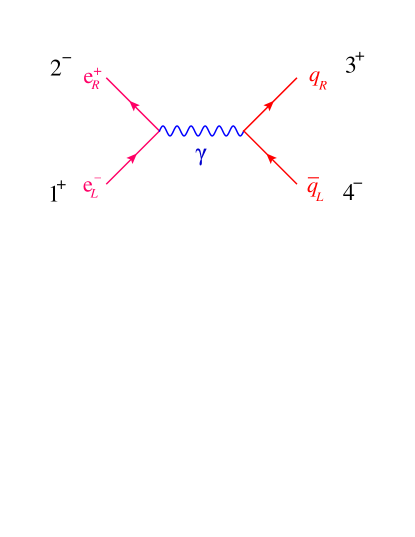
Figure 3: The one Feynman diagram for $e^{-}e^{+}\rightarrow q{\bar{q}}$. Particles are labeled with $L$ and $R$ subscripts for left- and right-handed particles. We also give in black the numerical, all-outgoing labeling convention.

We take all the external states to be helicity eigenstates, choosing first to consider,

$$e_{L}^{-}(-k_{1})e_{R}^{+}(-k_{2})\rightarrow q_{R}(k_{3}){\bar{q}}_{L}(k_{4})\,.$$ (28)

Note that we have assigned momenta $-k_{1}$ and $-k_{2}$ to the incoming states, so that momentum conservation takes the crossing-symmetric form,

$$k_{1}+k_{2}+k_{3}+k_{4}=0.$$ (29)

In the all-outgoing helicity labeling convention, the incoming left-handed electron is labeled as if it were an outgoing right-handed positron (positive-helicity $\bar{e}$), and similarly for the incoming right-handed positron (labeled as a negative-helicity $e$). We label the amplitude with numerals $i$ standing for the momenta $k_{i}$, subscripts to identify the type of particle (if it is not a gluon), and superscripts to indicate the helicity. Thus the amplitude for reaction (28) is denoted by

$${\cal A}_{4}^{\rm tree}(1_{\bar{e}}^{+},2_{e}^{-},3_{q}^{+},4_{\bar{q}}^{-})\equiv{\cal A}_{4}\,.$$ (30)

As discussed above, we first strip off the color factors, as well as any other coupling factors. In this case the color factor is a trivial Kronecker $\delta$ that equates the quark colors. We define the color-stripped amplitude $A_{4}$ by

$${\cal A}_{4}=(\sqrt{2}e)^{2}Q_{e}Q_{q}\delta_{i_{3}}^{{\bar{\imath}}_{4}}\,A_{4}\,,$$ (31)

where $e$ is the electromagnetic coupling, obeying $e^{2}/(4\pi)=\alpha_{\rm QED}$, and $Q_{e}$ and $Q_{q}$ are the electron and quark charges. The factor of $(\sqrt{2}e)^{2}$ arises because it is convenient to normalize the color-stripped amplitudes so that there are no $\sqrt{2}$ factors for QCD. In this normalization, the substitution $g\rightarrow\sqrt{2}e$ is required in the prefactor for each QED coupling. A corresponding $(1/\sqrt{2})^{2}$ goes into the Feynman rule for $A_{4}$.

The usual Feynman rules for the diagram in fig. 3 give

$$A_{4} = \frac{i}{2s_{12}}\overline{v_{-}}(k_{2})\gamma^{\mu}u_{-}(k_{1})\overline{u_{+}}(k_{3})\gamma_{\mu}v_{+}(k_{4})$$ (32)

$$= \frac{i}{2s_{12}}(\sigma^{\mu})_{\alpha\dot{\alpha}}(\lambda_{2})^{\alpha}(\tilde{\lambda}_{1})^{\dot{\alpha}}(\sigma_{\mu})^{\dot{\beta}\beta}(\tilde{\lambda}_{3})_{\dot{\beta}}(\lambda_{4})_{\beta}\,,$$

where we have switched to two-component notation in the second line. Now we apply the Fierz identity for Pauli matrices, eq. (17), obtaining

$$A_{4}\ =\ \frac{i}{s_{12}}(\lambda_{2})^{\alpha}(\tilde{\lambda}_{1})^{\dot{\alpha}}(\lambda_{4})_{\alpha}(\tilde{\lambda}_{3})_{\dot{\alpha}}\ =\ i\,\frac{\left\langle 2\,4\right\rangle\left[1\,3\right]}{s_{12}}\,,$$ (33)

after using the definitions (11) and (12) of the spinor products $\left\langle i\,j\right\rangle$ and $\left[i\,j\right]$.

According to eqs. (22) and (15), the spinor products are square-roots of the momentum invariants, up to a phase. Because $s_{24}=s_{13}$ for massless four-point kinematics, we can rewrite eq. (33) as

$$A_{4}\ =\ i\,\frac{\left\langle 2\,4\right\rangle\left[1\,3\right]}{s_{12}}\ =\ e^{i\phi}\frac{s_{13}}{s_{12}}\ =\ -\frac{e^{i\phi}}{2}(1-\cos\theta)\,,$$ (34)

where $\phi$ is some phase angle, and $\theta$ is the center-of-mass scattering angle. From this formula, we can check the helicity suppression of the amplitude in the forward scattering limit, $A_{4}\rightarrow 0$ as $\theta\rightarrow 0$. The amplitude vanishes in this limit because of angular-momentum conservation: the initial angular momentum along the $e_{L}^{-}$ direction is $(-\textstyle{1\over 2})-\textstyle{1\over 2}=-1$, while the final angular momentum is $\textstyle{1\over 2}-(-\textstyle{1\over 2})=+1$. At $\theta=\pi$, the spins line up and there is no suppression.

The result (33) for $A_{4}$ is in a mixed representation, containing both the “holomorphic” (right-handed) spinor product $\left\langle 2\,4\right\rangle$ and the “anti-holomorphic” (left-handed) spinor product $\left[1\,3\right]$. However, we can multiply top and bottom by $\left\langle 1\,3\right\rangle$, and use the squaring relation (22), $s_{13}=s_{24}$ and momentum conservation (23) to rewrite it as,

$$A_{4}=i\,\frac{\left\langle 2\,4\right\rangle\left[1\,3\right]}{s_{12}}=i\,\frac{\left\langle 2\,4\right\rangle\left[1\,3\right]\left\langle 1\,3\right\rangle}{\left\langle 1\,2\right\rangle\left[2\,1\right]\left\langle 1\,3\right\rangle}=-i\,\frac{\left\langle 2\,4\right\rangle\left[2\,4\right]\left\langle 2\,4\right\rangle}{\left\langle 1\,2\right\rangle\left[2\,4\right]\left\langle 4\,3\right\rangle}=i\,\frac{{\left\langle 2\,4\right\rangle}^{2}}{\left\langle 1\,2\right\rangle\left\langle 3\,4\right\rangle}\,.$$ (35)

The latter form only involves the spinors $\left\langle i\,j\right\rangle$. On the other hand, the same identities also allow us to write it in an anti-holomorphic form. In summary, we have

$$A_{4}^{\rm tree}(1_{\bar{e}}^{+},2_{e}^{-},3_{q}^{+},4_{\bar{q}}^{-})=i\,\frac{{\left\langle 2\,4\right\rangle}^{2}}{\left\langle 1\,2\right\rangle\left\langle 3\,4\right\rangle}=i\,\frac{{\left[1\,3\right]}^{2}}{\left[1\,2\right]\left[3\,4\right]}\,.$$ (36)

It turns out that $A_{4}^{\rm tree}(1_{\bar{e}}^{+},2_{e}^{-},3_{q}^{+},4_{\bar{q}}^{-})$ is the first in an infinite series of “maximally helicity violating” (MHV) amplitudes, containing these four fermions along with $(n-4)$ additional positive-helicity gluons or photons. All of these MHV amplitudes, containing exactly two negative-helicity particles, are holomorphic. (We will compute one of them in a little while.) But $A_{4}^{\rm tree}(1_{\bar{e}}^{+},2_{e}^{-},3_{q}^{+},4_{\bar{q}}^{-})$ is also the first in an infinite series of $\overline{\rm MHV}$ amplitudes, containing these four fermions along with $(n-4)$ additional negative-helicity gluons or photons. All the $\overline{\rm MHV}$ amplitudes are anti-holomorphic; in fact, they are the parity conjugates of the MHV amplitudes. As a four-point amplitude, eq. (36) has a dual life, belonging to both the MHV and the $\overline{\rm MHV}$ series. The same phenomenon occurs for other classes of amplitudes, including the $n$-gluon MHV amplitudes (the Parke-Taylor amplitudes [5]) and their $\overline{\rm MHV}$ conjugate amplitudes, which we will encounter shortly.

So far we have only computed one helicity configuration for $e^{+}e^{-}\rightarrow q{\bar{q}}$. There are 16 configurations in all. However, the helicity of massless fermions is conserved when they interact with gauge fields, or in the all-outgoing labeling, the positron’s helicity must be the opposite of the electron’s, and the antiquark’s helicity must be the opposite of the quark’s. So there are only $2\times 2=4$ nonvanishing helicity configurations. They are all related by parity (P) and by charge conjugation (C) acting on one of the fermion lines. For example, C acting on the electron line exchanges labels 1 and 2, which can also be interpreted as flipping the helicities of particles 1 and 2, taking us from eq. (36) to

$$A_{4}^{\rm tree}(1_{\bar{e}}^{-},2_{e}^{+},3_{q}^{+},4_{\bar{q}}^{-})=-i\,\frac{{\left\langle 1\,4\right\rangle}^{2}}{\left\langle 1\,2\right\rangle\left\langle 3\,4\right\rangle}\,.$$ (37)

Parity flips all helicities and conjugates all spinors, $\left\langle i\,j\right\rangle\rightarrow\left[i\,j\right]$, taking us from eq. (36) to

$$A_{4}^{\rm tree}(1_{\bar{e}}^{-},2_{e}^{+},3_{q}^{-},4_{\bar{q}}^{+})=i\,\frac{{\left[2\,4\right]}^{2}}{\left[1\,2\right]\left[3\,4\right]}\,.$$ (38)

Combining the two operations leads to

$$A_{4}^{\rm tree}(1_{\bar{e}}^{+},2_{e}^{-},3_{q}^{-},4_{\bar{q}}^{+})=-i\,\frac{{\left[1\,4\right]}^{2}}{\left[1\,2\right]\left[3\,4\right]}\,.$$ (39)

Of course eqs. (37), (38) and (39) can all be rewritten in the conjugate variables as well.

The scattering probability, or differential cross section, is proportional to the square of the amplitude. Squaring a single helicity amplitude would give the cross section for fully polarized incoming and outgoing particles. In QCD applications, we rarely have access to the spin states of the partons. Hadron beams are usually unpolarized, so the incoming quarks and gluons are as well. The outgoing quarks and gluons shower and fragment to produce jets of hadrons, wiping out almost all traces of final-state parton helicities. In other words, we need to construct the unpolarized cross section, by summing over all possible helicity configurations. (The different helicity configurations do not interfere with each other.) For our $e^{+}e^{-}\rightarrow q{\bar{q}}$ example, we need to sum over the four nonvanishing helicity configurations, after squaring the tree-level helicity amplitudes. The result, omitting the overall coupling and flux factors, is

$$\frac{d\sigma}{d\cos\theta}\ \propto\ \sum_{\rm hel.}|A_{4}|^{2}\ = \ 2\,\biggl{\{}\biggl{|}\frac{{\left\langle 2\,4\right\rangle}^{2}}{\left\langle 1\,2\right\rangle\left\langle 3\,4\right\rangle}\biggr{|}^{2}+\biggl{|}\frac{{\left\langle 1\,4\right\rangle}^{2}}{\left\langle 1\,2\right\rangle\left\langle 3\,4\right\rangle}\biggr{|}^{2}\biggr{\}}$$

$$= \ 2\,\frac{s_{24}^{2}+s_{14}^{2}}{s_{12}^{2}}$$

$$= \ \frac{1}{2}\Bigl{[}(1-\cos\theta)^{2}+(1+\cos\theta)^{2}\Bigr{]}$$

$$= \ 1+\cos^{2}\theta.$$ (40)

We used the fact that the amplitudes related by parity are equal up to a phase, in order to only exhibit two of the four nonzero helicity configurations explicitly.

For a simple process like $e^{+}e^{-}\rightarrow q{\bar{q}}$, helicity amplitudes are overkill. It would be much faster to use the textbook method of computing the unpolarized differential cross section directly, by squaring the amplitude for generic external spinors and using Casimir’s trick of inserting the positive energy projector for the product of two spinors, summed over spin states. The problem with this method is that the computational effort scales very poorly when there a large number of external legs $n$. The number of Feynman diagrams grows like $n!$, so the number of separate interferences between diagrams in the squared amplitude goes like $(n!)^{2}$. That is why all modern methods for high-multiplicity scattering processes compute amplitudes, not cross sections, for some basis of external polarization states. For massless particles, this is usually the helicity basis. After computing numerical values for the helicity amplitudes at a given phase-space point, the cross section is constructed from the helicity sum.

3.3 Helicity formalism for massless vectors

Next we consider external massless vector particles, i.e. gluons or photons. Spinor-helicity techniques began in the early 1980s with the recognition [2] that polarization vectors for massless vector particles with definite helicity could be constructed from a pair of massless spinors, as follows:

$$(\varepsilon_{i}^{+})_{\mu}=\varepsilon_{\mu}^{+}(k_{i},q) = \frac{\left\langle\smash{q}{\vphantom{1}}^{-}\right|{\gamma_{\mu}}\left|\smash{i}{\vphantom{1}}^{-}\right\rangle}{\sqrt{2}\left\langle q\,i\right\rangle}\,,\qquad(\varepsilon_{i}^{-})_{\mu}=\varepsilon_{\mu}^{-}(k_{i},q)=-\frac{\left\langle\smash{q}{\vphantom{1}}^{+}\right|{\gamma_{\mu}}\left|\smash{i}{\vphantom{1}}^{+}\right\rangle}{\sqrt{2}\left[q\,i\right]}\,,$$ (41)

$$(\not{\hbox{\kern-2.3pt$\varepsilon$}}_{i}^{+})_{\alpha\dot{\alpha}}=\,\not{\hbox{\kern-2.3pt$\varepsilon$}}_{\alpha\dot{\alpha}}^{+}(k_{i},q) = \sqrt{2}\frac{\lambda_{q}^{\alpha}\tilde{\lambda}_{i}^{\dot{\alpha}}}{\left\langle q\,i\right\rangle}\,,\qquad\ \ \ (\not{\hbox{\kern-2.3pt$\varepsilon$}}_{i}^{-})_{\alpha\dot{\alpha}}=\,\not{\hbox{\kern-2.3pt$\varepsilon$}}_{\alpha\dot{\alpha}}^{-}(k_{i},q)=-\sqrt{2}\frac{\tilde{\lambda}_{q}^{\dot{\alpha}}\lambda_{i}^{\alpha}}{\left[q\,i\right]}\,,$$ (42)

where we have also given the $2\times 2$ matrix version, from contracting with a $\sigma$ matrix and using the Fierz identity (17). Here $k_{i}^{\mu}$ is the gluon momentum and $q^{\mu}$ is an additional massless vector called the reference momentum, whose associated two-component left- and right-handed spinors are $\tilde{\lambda}_{q}^{\dot{\alpha}}$ and $\lambda_{q}^{\alpha}$. Using the massless Dirac equation,

$$\not{\hbox{\kern-2.3pt$k$}}_{i}|i^{\pm}\rangle\ =\ 0\ =\ \not{\hbox{\kern-2.3pt$q$}}|q^{\pm}\rangle\,,$$ (43)

we see that the polarization vectors (41) obey the required transversality with respect the gluon momentum,

$$\varepsilon_{i}^{\pm}\cdot k_{i}=0\,.$$ (44)

As a bonus, it also is transverse with respect to $q$: $\varepsilon_{i}^{\pm}\cdot q=0$.

The second form (42) for the polarization vector shows that $\not{\hbox{\kern-2.3pt$\varepsilon$}}_{i}^{+}$ produces a state with helicity $+1$, because it contains two complex conjugate spinors with momentum $k_{i}$ in the numerator and denominator. These two spinors pick up opposite spin-$1/2$ phases under an azimuthal rotation about the $k_{i}$ axis,

$$\tilde{\lambda}_{i}^{\dot{\alpha}}\rightarrow e^{i\phi/2}\tilde{\lambda}_{i}^{\dot{\alpha}}\,,\qquad\lambda_{i}^{\alpha}\rightarrow e^{-i\phi/2}\lambda_{i}^{\alpha}\,,$$ (45)

so the ratio transforms like helicity $+1$,

$$\not{\hbox{\kern-2.3pt$\varepsilon$}}_{i}^{+}\propto\frac{\tilde{\lambda}_{i}^{\dot{\alpha}}}{\lambda_{i}^{\alpha}}\ \rightarrow\ e^{i\phi}\not{\hbox{\kern-2.3pt$\varepsilon$}}_{i}^{+}\,.$$ (46)

There is a freedom to choose different reference vectors $q_{i}$ for each of the external states $i$. This freedom is the residual on-shell gauge invariance, that amplitudes should be unchanged when the polarization vector is shifted by an amount proportional to the momentum. A judicious choice of the reference vectors can greatly simplify a Feynman diagram computation by causing many diagrams to vanish. However, we won’t be doing many Feynman diagram computations, just the one in the next subsection, of a five-point amplitude. In this case, there are only two diagrams, one of which we will make vanish through a choice of $q$.

3.4 A five-point amplitude

In this subsection we compute one of the next simplest helicity amplitudes, the one for producing a gluon along with the quark-antiquark pair in $e^{+}e^{-}$ annihilation. This amplitude contributes to three-jet production in $e^{+}e^{-}$ annihilation, and to the next-to-leading order corrections to deep inelastic scattering and to Drell-Yan production, in the crossed channels.

We compute the amplitude for the helicity configuration

$$e_{L}^{-}(-k_{1})e_{R}^{+}(-k_{2})\rightarrow q_{R}(k_{3})g_{R}(k_{4}){\bar{q}}_{L}(k_{5})\,,$$ (47)

namely

$${\cal A}_{5}^{\rm tree}(1_{\bar{e}}^{+},2_{e}^{-},3_{q}^{+},4^{+},5_{\bar{q}}^{-})\equiv{\cal A}_{5}\,.$$ (48)

Again we strip off the color and charge factors, defining

$${\cal A}_{5}=(\sqrt{2}e)^{2}g\,Q_{e}Q_{q}(T^{a_{4}})_{i_{3}}^{{\bar{\imath}}_{5}}\,A_{5}\,,$$ (49)

where $A_{5}$ is constructed from the two Feynman diagrams in fig. 4.

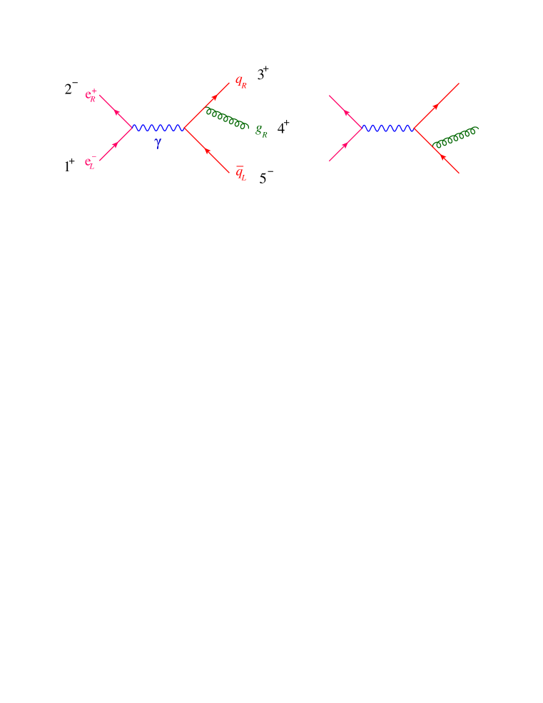
Figure 4: The two Feynman diagrams for $e^{-}e^{+}\rightarrow qg{\bar{q}}$.

Recall that in the evaluation of the four-point amplitude (33), after applying the Fierz identity related to the photon propagator, the two external fermions with the same (outgoing) helicity had their spinors contracted together, generating factors of $\left\langle 2\,4\right\rangle$ and $\left[1\,3\right]$. In the two diagrams in fig. 4, the same thing happens for the quark or anti-quark that does not have a gluon emitted off it, generating a factor of $\left\langle 2\,5\right\rangle$ in the first diagram and $\left[1\,3\right]$ in the second one. On the other spinor string, we have to insert a factor of the off-shell fermion propagator and the gluon polarization vector, giving

$$A_{5}=-i\,\frac{\left\langle 2\,5\right\rangle}{s_{12}}\frac{\left\langle\smash{1}{\vphantom{1}}^{+}\right|{(\not{\hbox{\kern-2.3pt$k$}}_{3}+\not{\hbox{\kern-2.3pt$k$}}_{4})\not{\hbox{\kern-2.3pt$\varepsilon$}}_{4}^{+}}\left|\smash{3}{\vphantom{1}}^{-}\right\rangle}{\sqrt{2}s_{34}}+i\,\frac{\left[1\,3\right]}{s_{12}}\frac{\left\langle\smash{2}{\vphantom{1}}^{-}\right|{(\not{\hbox{\kern-2.3pt$k$}}_{4}+\not{\hbox{\kern-2.3pt$k$}}_{5})\not{\hbox{\kern-2.3pt$\varepsilon$}}_{4}^{+}}\left|\smash{5}{\vphantom{1}}^{+}\right\rangle}{\sqrt{2}s_{45}}\,.$$ (50)

Inserting the formula (42) for the gluon polarization vector, we obtain

$$A_{5}=-i\,\frac{\left\langle 2\,5\right\rangle}{s_{12}}\frac{\left\langle\smash{1}{\vphantom{1}}^{+}\right|{(\not{\hbox{\kern-2.3pt$k$}}_{3}+\not{\hbox{\kern-2.3pt$k$}}_{4})}\left|\smash{q}{\vphantom{1}}^{+}\right\rangle\left[4\,3\right]}{s_{34}\left\langle q\,4\right\rangle}+i\,\frac{\left[1\,3\right]}{s_{12}}\frac{\left\langle\smash{2}{\vphantom{1}}^{-}\right|{(\not{\hbox{\kern-2.3pt$k$}}_{4}+\not{\hbox{\kern-2.3pt$k$}}_{5})}\left|\smash{4}{\vphantom{1}}^{-}\right\rangle\left\langle q\,5\right\rangle}{s_{45}\left\langle q\,4\right\rangle}\,.$$ (51)

Now we choose the reference momentum $q=k_{5}$ in order to make the second graph vanish,

$$A_{5}=-i\,\frac{\left\langle 2\,5\right\rangle}{s_{12}}\frac{\left\langle\smash{1}{\vphantom{1}}^{+}\right|{(\not{\hbox{\kern-2.3pt$k$}}_{3}+\not{\hbox{\kern-2.3pt$k$}}_{4})}\left|\smash{5}{\vphantom{1}}^{+}\right\rangle\left[4\,3\right]}{s_{34}\left\langle 5\,4\right\rangle}=-i\,\frac{\left\langle 2\,5\right\rangle\left[1\,2\right]\left\langle 2\,5\right\rangle\left[4\,3\right]}{\left\langle 1\,2\right\rangle\left[2\,1\right]\left\langle 3\,4\right\rangle\left[4\,3\right]\left\langle 4\,5\right\rangle}=i\,\frac{{\left\langle 2\,5\right\rangle}^{2}}{\left\langle 1\,2\right\rangle\left\langle 3\,4\right\rangle\left\langle 4\,5\right\rangle}\,,$$ (52)

where we used momentum conservation (23) and a couple of other spinor-product identities to simplify the answer to its final holomorphic form,

$$A_{5}(1_{\bar{e}}^{+},2_{e}^{-},3_{q}^{+},4^{+},5_{\bar{q}}^{-})=i\,\frac{{\left\langle 2\,5\right\rangle}^{2}}{\left\langle 1\,2\right\rangle\left\langle 3\,4\right\rangle\left\langle 4\,5\right\rangle}\,.$$ (53)

(As an exercise in spinor-product identities, verify eq. (53) for other choices of $q$.)

Next we will study the behavior of $A_{5}$ in various kinematic limits, which will give us insight into the generic singular behavior of QCD amplitudes.

4 Soft and collinear factorization

In this section, we use the five-point amplitude (53) to verify some universal limiting behavior of QCD amplitudes. In the next section, we will use this universal behavior to derive recursion relations for general tree amplitudes.

4.1 Soft gluon limit

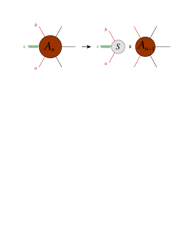
Figure 5: Factorization of a QCD amplitude when a soft gluon $s$ is emitted between the hard partons $a$ and $b$.

First consider the limit that the gluon momentum $k_{4}$ in eq. (53) becomes soft, i.e. scales uniformly to zero, $k_{4}\rightarrow 0$. In this limit, we can factorize the amplitude into a divergent piece that depends on the energy and angle of the emitted gluon, and a second piece which is the amplitude omitting that gluon:

$$A_{5}(1_{\bar{e}}^{+},2_{e}^{-},3_{q}^{+},4^{+},5_{\bar{q}}^{-})=i\,\frac{{\left\langle 2\,5\right\rangle}^{2}}{\left\langle 1\,2\right\rangle\left\langle 3\,4\right\rangle\left\langle 4\,5\right\rangle} = \frac{\left\langle 3\,5\right\rangle}{\left\langle 3\,4\right\rangle\left\langle 4\,5\right\rangle}\times i\,\frac{{\left\langle 2\,5\right\rangle}^{2}}{\left\langle 1\,2\right\rangle\left\langle 3\,5\right\rangle}$$ (54)

$$\rightarrow {\cal S}(3,4^{+},5)\times A_{4}(1_{\bar{e}}^{+},2_{e}^{-},3_{q}^{+},5_{\bar{q}}^{-})\,.$$

The soft factor (or eikonal factor) is given more generally by,

$${\cal S}(a,s^{+},b)=\frac{\left\langle a\,b\right\rangle}{\left\langle a\,s\right\rangle\left\langle s\,b\right\rangle}\,,\qquad{\cal S}(a,s^{-},b)=-\frac{\left[a\,b\right]}{\left[a\,s\right]\left[s\,b\right]}\,,$$ (55)

where $s$ labels the soft gluon, and $a$ and $b$ label the two hard partons that are adjacent to it in the color ordering.

Although we have only inspected the soft limit of one amplitude, the more general result is,

$$A_{n}^{\rm tree}(1,2,\ldots,a,s^{\pm},b,\ldots,n)\buildrel k_{s}\rightarrow 0\over{\relbar\mskip-0.5mu\joinrel\mskip-0.5mu\relbar\mskip-0.5mu\joinrel\longrightarrow}\ {\cal S}(a,s^{\pm},b)\times A_{n-1}^{\rm tree}(1,2,\ldots,a,b,\ldots,n)\,.$$ (56)

This factorization is depicted in fig. 5. The $(n-1)$-point amplitude on the right-hand side is that obtained by just deleting the soft-gluon $s$ in the $n$-point amplitude. The soft factor is universal: it does not depend on whether $a$ and $b$ are quarks or gluons; it does not care about their helicity; and it does not even depend on the magnitude of their momenta, just their angular direction (as one can see by rescaling the spinor $\lambda_{a}$ in eq. (55)). The spin independence arises because soft emission is long-wavelength, and intrinsically classical. Because of this, we can pretend that the external partons $a$ and $b$ are scalars, and compute the soft factor simply from two Feynman diagrams, from emission off legs $a$ and $b$. We can use the scalar QED vertex in the numerator, while the (singular) soft limit of the adjacent internal propagator generates the denominator:

$${\cal S}(a,s^{+},b)=-\frac{\sqrt{2}\varepsilon_{s}^{+}(q)\cdot k_{a}}{2k_{a}\cdot k_{s}}+\frac{\sqrt{2}\varepsilon_{s}^{+}(q)\cdot k_{b}}{2k_{b}\cdot k_{s}}=\frac{\left\langle a\,q\right\rangle}{\left\langle s\,q\right\rangle\left\langle a\,s\right\rangle}-\frac{\left\langle b\,q\right\rangle}{\left\langle s\,q\right\rangle\left\langle b\,s\right\rangle}=\frac{\left\langle a\,b\right\rangle}{\left\langle a\,s\right\rangle\left\langle s\,b\right\rangle}\,,$$ (57)

using the Schouten identity (24) in the last step.

4.2 Collinear limits

Next consider the limit of the $e^{+}e^{-}\rightarrow qg\bar{q}$ amplitude (53) as the quark momentum $k_{3}\equiv k_{a}$ and the gluon momentum $k_{4}\equiv k_{b}$ become parallel, or collinear. This limit is singular because the intermediate momentum $k_{P}\equiv k_{a}+k_{b}$ is going on shell in the collinear limit:

$$k_{P}^{2}=2k_{a}\cdot k_{b}\buildrel a\parallel b\over{\relbar\mskip-0.5mu\joinrel\mskip-0.5mu\relbar\mskip-0.5mu\joinrel\longrightarrow}0.$$ (58)

We also need to specify the relative longitudinal momentum fractions carried by partons $a$ and $b$,

$$k_{a}\approx zk_{P}\,,\qquad k_{b}\approx(1-z)k_{P}\,,$$ (59)

where $0<z<1$. This relation implies, thanks to eq. (26), that the spinors obey similar relations with square roots:

$$\lambda_{a}\approx\sqrt{z}\,\lambda_{P}\,,\qquad\lambda_{b}\approx\sqrt{1-z}\,\lambda_{P}\,,$$ (60)

$$\tilde{\lambda}_{a}\approx\sqrt{z}\,\tilde{\lambda}_{P}\,,\qquad\tilde{\lambda}_{b}\approx\sqrt{1-z}\,\tilde{\lambda}_{P}\,,$$ (61)

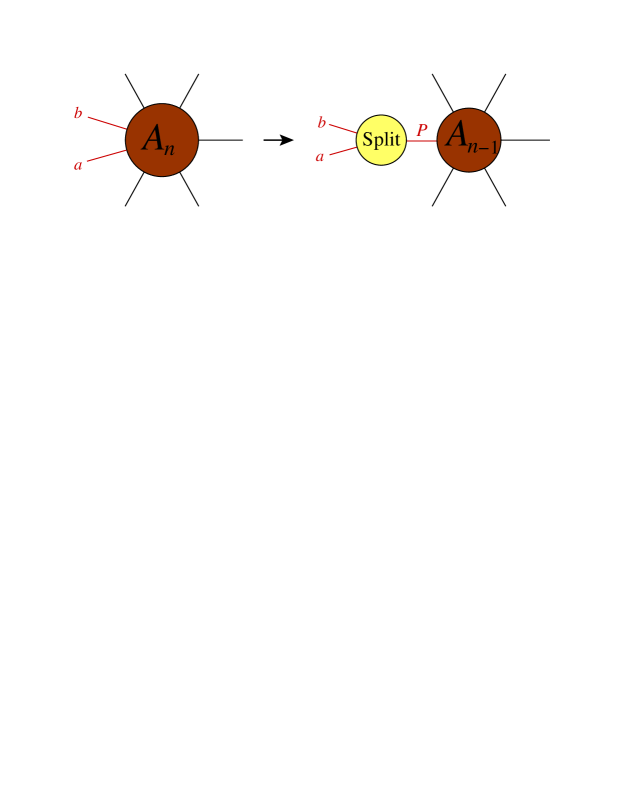
Figure 6: Factorization of a QCD amplitude when two color-adjacent partons $a$ and $b$ become collinear.

Inserting eq. (60) into eq. (53), we find that

$$A_{5}(1_{\bar{e}}^{+},2_{e}^{-},3_{q}^{+},4^{+},5_{\bar{q}}^{-})=i\,\frac{{\left\langle 2\,5\right\rangle}^{2}}{\left\langle 1\,2\right\rangle\left\langle 3\,4\right\rangle\left\langle 4\,5\right\rangle} \approx \frac{1}{\sqrt{1-z}\left\langle 3\,4\right\rangle}\times i\,\frac{{\left\langle 2\,5\right\rangle}^{2}}{\left\langle 1\,2\right\rangle\left\langle P\,5\right\rangle}$$

$$\rightarrow \mathop{\rm Split}\nolimits_{-}(3_{q}^{+},4_{g}^{+};z)\times A_{4}(1_{\bar{e}}^{+},2_{e}^{-},P_{q}^{+},5_{\bar{q}}^{-})\,.$$

Here we have introduced the splitting amplitude $\mathop{\rm Split}\nolimits_{-\lambda_{P}}(a^{\lambda_{a}},b^{\lambda_{b}};z)$, which governs the general collinear factorization of tree amplitudes depicted in fig. 6,

$$A_{n}^{\rm tree}(\ldots,a^{\lambda_{a}},b^{\lambda_{b}},\ldots)\buildrel a\parallel b\over{\relbar\mskip-0.5mu\joinrel\mskip-0.5mu\relbar\mskip-0.5mu\joinrel\longrightarrow}\ \sum_{\lambda_{P}=\pm}\mathop{\rm Split}\nolimits_{-\lambda_{P}}(a^{\lambda_{a}},b^{\lambda_{b}};z)\,A_{n-1}^{\rm tree}(\ldots,P^{\lambda_{P}},\ldots)\,.$$ (63)

In contrast to the soft factor, the splitting amplitude depends on whether $a$ and $b$ are quarks or gluons, and on their helicity. It also includes a sum over the helicity $\lambda_{P}$ of the intermediate parton $P$. (Note that the labeling of $\lambda_{P}$ is reversed between the $(n-1)$-point tree amplitude and the splitting amplitude, because we apply the all-outgoing helicity convention to the splitting amplitude as well.) The $(n-1)$-point tree amplitude on the right-hand side of eq. (63) is found by merging the two partons, according to the possible splittings in QCD: $g\rightarrow gg$, $g\rightarrow q\bar{q}$, $\bar{q}\rightarrow\bar{q}g$ and (in this case) $q\rightarrow qg$. For the splitting amplitude $\mathop{\rm Split}\nolimits_{-}(a_{q}^{+},b_{g}^{+};z)$ entering eq. (LABEL:A5coll34), quark helicity conservation implies that only one of the two intermediate helicities survives. For intermediate gluons, both signs of $\lambda_{P}$ can appear in general. As in the case of the soft limit, the four-point amplitude $A_{4}$ is found by relabeling eq. (36).

One can also extract from eq. (53) the splitting amplitude for the case that the (anti)quark and gluon have the opposite helicity, by taking the collinear limit $4\parallel 5$. The two results can be summarized as:

$$\mathop{\rm Split}\nolimits_{-}(q^{+},g^{+}) = \frac{1}{\sqrt{1-z}\left\langle q\,g\right\rangle}\,,\qquad\mathop{\rm Split}\nolimits_{-}(q^{+},g^{-})=-\frac{z}{\sqrt{1-z}\left[q\,g\right]}\,,$$ (64)

$$\mathop{\rm Split}\nolimits_{-}(g^{+},{\bar{q}}^{+}) = \frac{1}{\sqrt{z}\left\langle g\,{\bar{q}}\right\rangle}\,,\qquad\mathop{\rm Split}\nolimits_{-}(g^{-},{\bar{q}}^{+})=-\frac{1-z}{\sqrt{z}\left[g\,{\bar{q}}\right]}\,.$$ (65)

where the other cases (including some not shown, with opposite quark helicity) are related by parity or charge conjugation.

Collinear singularities in the initial state give rise to the DGLAP evolution equations for parton distributions. In fact, the splitting amplitudes are essentially the square root of the (polarized) Altarelli-Parisi splitting probabilities which are the kernels of the DGLAP equations. That is, the $z$ dependence of the splitting amplitudes, after squaring and summing over the helicities $\lambda_{a}$, $\lambda_{b}$ and $\lambda_{P}$, reproduces the splitting probabilities. For example, one can reconstruct the correct $z$-dependence of the $q\rightarrow qg$ splitting probabilities $P_{qq}(z)$ using eq. (64), squaring and summing over the gluon helicity:

$$P_{qq}(z)\ \propto\ \left(\frac{1}{\sqrt{1-z}}\right)^{2}+\left(\frac{z}{\sqrt{1-z}}\right)^{2}\ =\ \frac{1+z^{2}}{1-z}\,,$$ (66)

while $P_{gq}(z)$ is given by exchanging $z\leftrightarrow 1-z$. Equation (66) omits the $\delta(1-z)$ term from virtual gluon emission, but its coefficient can be inferred from quark number conservation.

4.3 The Parke-Taylor amplitudes

In the all-outgoing helicity convention, one can show that the pure-gluon amplitudes for which all the gluon helicities are the same, or at most one is different from the rest, vanish for any $n\geq 4$:

$$A_{n}^{\rm tree}(1^{\pm},2^{+},\ldots,n^{+})=0.$$ (67)

(Cyclic symmetry allows us to move a single negative-helicity gluon to leg 1.) This result can be proven directly by noticing that the tree amplitude contains $n$ different polarization vectors, contracted together with at most $n-2$ momenta (because there are at most $n-2$ cubic vertices in any Feynman graph, each of which is linear in the momentum). Therefore every term in every tree amplitude contains at least one polarization vector contraction of the form $\varepsilon_{i}\cdot\varepsilon_{j}$. Inspecting the form of the polarization vectors in eq. (41), we see that like-helicity contractions, $\varepsilon_{i}^{+}(q_{i})\cdot\varepsilon_{j}^{+}(q_{j})$, vanish if $q_{i}=q_{j}$, while opposite helicity contractions, $\varepsilon_{i}^{-}(q_{i})\cdot\varepsilon_{j}^{+}(q_{j})$, vanish if $q_{i}=k_{j}$ or $q_{j}=k_{i}$. To show that $A_{n}^{\rm tree}(1^{+},2^{+},\ldots,n^{+})$ vanishes, we can just choose all reference momenta to be the same, $q_{i}=q$. To show that $A_{n}^{\rm tree}(1^{-},2^{+},\ldots,n^{+})$ vanishes, we can choose $q_{i}=k_{1}$ for $i>1$ and $q_{1}=k_{2}$, for example. It is also possible to prove eq. (67) using the fact that tree-level $n$-gluon amplitudes are the same in QCD as in a supersymmetric theory [4], and so they obey Ward identities for supersymmetric scattering amplitudes [3].

The remarkable simplicity of gauge-theory scattering amplitudes is encapsulated by the Parke-Taylor [5] amplitudes for the MHV $n$-gluon amplitudes, in which exactly two gluons, $j$ and $l$, have opposite helicity from the rest:

$$A_{jl}^{\rm MHV}\ \equiv\ A_{n}^{\rm tree}(1^{+},\ldots,j^{-},\ldots,l^{-},\ldots,n^{+})\ =\ i\,{{\left\langle j\,l\right\rangle}^{4}\over\left\langle 1\,2\right\rangle\cdots\left\langle n\,1\right\rangle}\ .$$ (68)

One of the reasons these amplitudes are so simple is that they have no multi-particle poles — no factors of $1/(k_{m}+k_{m+1}+\cdots+k_{p})^{2}\equiv 1/P^{2}$ for $p>m+1$. Why is that? A multi-particle pole would correspond to factorizing the scattering process into two subprocesses, each with at least four gluons,

$$A_{n}^{\rm tree}(\ldots)\ \buildrel P^{2}\rightarrow 0\over{\relbar\mskip-0.5mu\joinrel\mskip-0.5mu\relbar\mskip-0.5mu\joinrel\longrightarrow}\ A_{n-k+1}(\ldots,P^{\lambda_{P}},\ldots)\frac{i}{P^{2}}A_{k+1}(\ldots,(-P)^{-\lambda_{P}},\ldots)\,,\quad 3\leq k\leq n-3,$$ (69)

In the MHV case, there are two negative-helicity gluons among the arguments “$\ldots$” of the two tree amplitudes on the right-hand side of eq. (69), plus one more for either $P$ or $(-P)$ (but not both). That’s three negative-helicity gluons to be distributed among two tree amplitudes. However, eq. (67) says that both trees need at least two negative helicities to be nonvanishing, for a minimum of four required. Hence the multiparticle poles must all vanish, due to insufficiently many negative helicities. As we’ll see in section 6, similar arguments control the structure of loop amplitudes as well.

We have found that the MHV amplitudes have no multi-particle factorization poles, consistent with eq. (68). Their principal singularities are the soft and collinear limits. It’s easy to check that the soft limit (56) is satisfied by the MHV amplitudes in eq. (68). It’s also simple to verify that the collinear behavior (63) is obeyed, and to extract the $g\rightarrow gg$ splitting amplitudes,

$$\mathop{\rm Split}\nolimits_{-}(a^{+},b^{+}) = \frac{1}{\sqrt{z(1-z)}\left\langle a\,b\right\rangle}\,,\quad\mathop{\rm Split}\nolimits_{+}(a^{-},b^{+})=\frac{z^{2}}{\sqrt{z(1-z)}\left\langle a\,b\right\rangle}\,,$$

$$\mathop{\rm Split}\nolimits_{+}(a^{+},b^{-}) = \frac{z^{2}}{\sqrt{z(1-z)}\left\langle a\,b\right\rangle}\,,\quad\mathop{\rm Split}\nolimits_{+}(a^{+},b^{+})=0\,,$$ (70)

plus their parity conjugates. The last relation in eq. (70) must hold for consistency, because otherwise the collinear limit of an MHV amplitude (which has no multi-particle poles) could generate a next-to-MHV amplitude with three negative helicities (which generically does have such poles). It’s a useful exercise to reconstruct the unpolarized $g\rightarrow gg$ splitting probabilities $P_{gg}(z)$ from eq. (70) by squaring and summing over all helicity configurations.

A closely related series of MHV amplitudes to the pure-glue ones are those with a single external $q\bar{q}$ pair and $(n-2)$ gluons. In this case helicity conservation along the fermion line forces either the quark or antiquark to have negative helicity. Using charge conjugation, we can pick it to be the antiquark. Referring to the color decomposition (6), the partial amplitudes for which all gluons have the same helicity vanish identically,

$$A_{n}^{\rm tree}(1_{\bar{q}}^{-},2_{q}^{+},3^{+},4^{+},\ldots,n^{+})=0,$$ (71)

while the MHV ones with exactly one negative-helicity gluon (leg $i$) take the simple form,

$$A_{n}^{\rm tree}(1_{\bar{q}}^{-},2_{q}^{+},3^{+},\ldots,i^{-},\ldots,n^{+})\ =\ i\,{{\left\langle 1\,i\right\rangle}^{3}\left\langle 2\,i\right\rangle\over\left\langle 1\,2\right\rangle\cdots\left\langle n\,1\right\rangle}\,.$$ (72)

It’s easy to see that the absence of multi-particle poles in eq. (68), whether for intermediate gluons or quarks, again follows from the vanishing relations (67) and (71), and simple counting of negative helicities. However, the relation between the pure-glue MHV amplitudes $A_{1i}^{{\rm tree},{\rm MHV}}$ in eq. (68) and the quark-glue ones (72) is much closer than that, as they differ only by a factor of $\left\langle 2\,i\right\rangle/\left\langle 1\,i\right\rangle$. These relations follow from supersymmetry Ward identities [3, 4, 15, 16].

4.4 Spinor magic

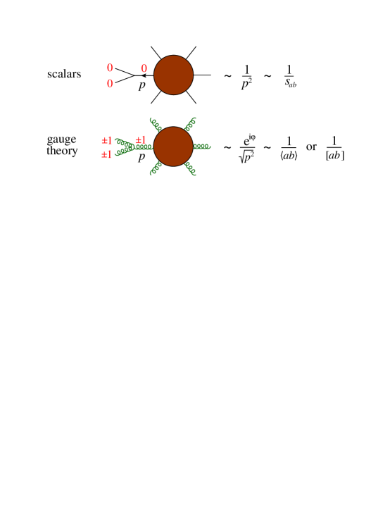
Figure 7: In gauge theory, an angular-momentum mismatch lessens the singular behavior from $1/p^{2}$ to $1/\sqrt{p^{2}}$, and introduces an azimuthally-dependent phase, both of which are captured by the spinor products.

All of the splitting amplitudes contain denominator factors of either $\left\langle a\,b\right\rangle$ or its parity conjugate $\left[a\,b\right]$. From eq. (20), we see that the collinear singularity is proportional to the square root of the momentum invariant that is vanishing, times a phase. This phase varies as the two collinear partons are rotated in the azimuthal direction about their common axis. Both the square root and the phase behavior follow from angular momentum conservation in the collinear limit. Figure 7 illustrates the difference between scalar $\phi^{3}$ theory and gauge theory. In scalar $\phi^{3}$ theory, no spin angular momentum is carried by either the external scalars or the intermediate one. Thus there is no violation of angular-momentum conservation along the collinear axis. Related to this, the three-vertex shown carries no momentum dependence, and the collinear pole is determined solely by the scalar propagator to be $\sim 1/s_{ab}$ in the limit that legs $a$ and $b$ become parallel.

In contrast, in every collinear limit in massless gauge theory, angular momentum conservation is violated by at least one unit. In the pure-glue case shown in fig. 7, the intermediate physical gluon must be transverse and have helicity $\pm 1$, but this value is never equal to the sum of the two external helicities: $\pm 1\pm 1=\pm 2$ or 0. The helicity mismatch forces the presence of orbital angular momentum, which comes from the momentum dependence in the gauge-theory three-vertex. It suppresses the amplitude in the collinear limit, from $1/s_{ab}$ to $1/\sqrt{s_{ab}}$, similarly to the vanishing of $A_{4}$ in eq. (34) in the limit $\theta\rightarrow 0$. The helicity mismatch also generates the azimuthally-dependent phase. The sign of the mismatch, by $\pm 1$ unit, is correlated with whether the splitting amplitude contains $1/\left\langle a\,b\right\rangle$ or $1/\left[a\,b\right]$, since these spinor products acquire opposite phases under an azimuthal rotation.

In summary, the spinor products are the perfect variables for capturing the collinear behavior of massless gauge theory amplitudes, simply due to angular-momentum considerations. Because collinear singularities dictate many of the denominator factors that should appear in the analytic representations of amplitudes, we can now understand more physically why the spinor product representation can lead to such compact analytic results.

4.5 Complex momenta, spinor products and three-point kinematics

There is another reason the spinor products are essential for modern amplitude methods, and that is to make sense out of massless three-point scattering. If we use only momentum invariants, then the three-point kinematics, defined by

$$k_{1}^{\mu}+k_{2}^{\mu}+k_{3}^{\mu}=0,\qquad k_{1}^{2}=k_{2}^{2}=k_{3}^{2}=0,$$ (73)

is pathological. For example, $s_{12}=(k_{1}+k_{2})^{2}=k_{3}^{2}=0$, and similarly every momentum invariant $s_{ij}$ vanishes. If the momenta are real, then eq. (20) implies that all the spinor products vanish as well, $\left\langle i\,j\right\rangle=\left[i\,j\right]=0$. It is easy to see that for real momenta the only solutions to eq. (73) consist of strictly parallel four-vectors, which is another way of seeing why all dot products and spinor products must vanish.

However, if the momenta are complex, there is a loophole: The conjugation relation (15), $\left[i\,j\right]=\left\langle i\,j\right\rangle^{\ast}$, does not hold, although the relation (19), $s_{ij}=\left\langle i\,j\right\rangle\left[j\,i\right]$, is still true. Therefore we can have some of the spinor products be nonzero, even though all the momentum invariants vanish, $s_{ij}=0$. There are two chirally conjugate solutions:

1. $\tilde{\lambda}_{1}\propto\tilde{\lambda}_{2}\propto\tilde{\lambda}_{3}\quad\Rightarrow\quad$all $\left[i\,j\right]=0$ while all $\left\langle i\,j\right\rangle\neq 0$.

2. $\lambda_{1}\propto\lambda_{2}\propto\lambda_{3}\quad\Rightarrow\quad$all $\left\langle i\,j\right\rangle=0$ while all $\left[i\,j\right]\neq 0$.

The proportionality of the two-component spinors causes the corresponding spinor products to vanish. There are no continuous variables associated with the three-point process, so one should think of the kinematical region as consisting of just two points, which are related to each other by parity.

For the first choice of kinematics, MHV three-point amplitudes such as

$$A_{3}^{\rm tree}(1^{-},2^{-},3^{+})=i\frac{{\left\langle 1\,2\right\rangle}^{4}}{\left\langle 1\,2\right\rangle\left\langle 2\,3\right\rangle\left\langle 3\,1\right\rangle}$$ (74)

make sense and are nonvanishing. $\overline{\rm MHV}$ three-point amplitudes such as

$$A_{3}^{\rm tree}(1^{+},2^{+},3^{-})=-i\frac{{\left[1\,2\right]}^{4}}{\left[1\,2\right]\left[2\,3\right]\left[3\,1\right]}$$ (75)

are nonvanishing for the second type of kinematics. When the MHV three-point amplitudes are nonvanishing, the $\overline{\rm MHV}$ ones vanish, and vice versa.

It’s important to note that the splitting amplitudes defined in section 4.2 correspond to approximate three-point kinematics with real momenta, whereas the three-point amplitudes (74) and (75) correspond to exact three-point kinematics with complex momenta. They are similar notions, but not exactly the same thing.

5 The BCFW recursion relation for tree amplitudes

5.1 General formula

The idea behind the derivation of the BCFW recursion relation [25] is that tree-level amplitudes are plastic, or continuously deformable, analytic functions of the scattering momenta. Therefore, it should be possible to reconstruct amplitudes for generic scattering kinematics from their behavior in singular limiting kinematics. In these singular regions, amplitudes split, or factorize, into two causally disconnected amplitudes with fewer legs, connected by a single intermediate state, which can propagate an arbitrary distance because it is on its mass shell.

Multi-leg amplitudes depend on many variables, and multi-variable complex analysis can be tricky. However, BCFW considered a family of on-shell tree amplitudes, $A_{n}(z)$, depending on a single complex parameter $z$ which shifts some of the momenta. (We drop the “tree” superscript here for convenience.) This family explores enough of the singular kinematical configurations to allow recursion relations to be derived for the original amplitude at $z=0$, $A_{n}=A_{n}(0)$. There have since been many generalizations of this approach, leading to different types of recursion relations. The BCFW momentum shift only affects two of the momenta, say legs $n$ and $1$. The shift can be defined using the spinor variables as,

$$\tilde{\lambda}_{n} \rightarrow \hat{\tilde{\lambda}}_{n}=\tilde{\lambda}_{n}-z\tilde{\lambda}_{1}\,,\qquad\lambda_{n}\rightarrow\lambda_{n}\,,$$

$$\lambda_{1} \rightarrow \hat{\lambda}_{1}=\lambda_{1}+z\lambda_{n}\,,\qquad\tilde{\lambda}_{1}\rightarrow\tilde{\lambda}_{1}\,,$$ (76)

where hatted variables indicate variables after the shift. This particular shift is called the $[n,1\rangle$ shift, because it only affects the spinor products involving the left-handed spinor $\tilde{\lambda}_{n}$ and the right-handed spinor $\lambda_{1}$.

The shift (76) can also be expressed in terms of momentum variables,

$$\hat{\not{\hbox{\kern-2.3pt$k$}}}_{1}(z)\ = \ (\lambda_{1}+z\lambda_{n})\,\tilde{\lambda}_{1}\ =\ \lambda_{1}\tilde{\lambda}_{1}+z\lambda_{n}\tilde{\lambda}_{1}\,,$$

$$\hat{\not{\hbox{\kern-2.3pt$k$}}}_{n}(z)\ = \ \lambda_{n}\,(\tilde{\lambda}_{n}-z\tilde{\lambda}_{1})\ =\ \lambda_{n}\tilde{\lambda}_{n}-z\lambda_{n}\tilde{\lambda}_{1}\,,$$ (77)

which makes clear that momentum conservation holds for any value of $z$, because

$$\hat{k}_{1}^{\mu}(z)+\hat{k}_{n}^{\mu}(z)=k_{1}^{\mu}+k_{n}^{\mu}\,.$$ (78)

Also, since both $\hat{\not{\hbox{\kern-2.3pt$k$}}}_{1}(z)$ and $\hat{\not{\hbox{\kern-2.3pt$k$}}}_{n}(z)$ in eq. (77) can be factorized as $2\times 2$ matrices into row vectors times column vectors, their determinants vanish. Then, according to the discussion around eq. (14), they remain on shell,

$$\hat{k}_{1}^{2}(z)=\hat{k}_{n}^{2}(z)=0.$$ (79)

We can give a physical picture of the direction of the momentum shift by first writing $\hat{k}_{1}^{\mu}(z)=k_{1}^{\mu}+zv^{\mu}$, $\hat{k}_{n}^{\mu}(z)=k_{1}^{\mu}-zv^{\mu}$. Requiring eq. (79) for all $z$ implies that $v\cdot k_{1}=v\cdot k_{n}=v^{2}=0$. If we go to a Lorentz frame in which the spatial components of $k_{1}$ and $k_{n}$ are both along the $z$ direction, then we see that $v^{\mu}$ must be a null vector in the space-like transverse $(x,y)$ plane. This is only possible if $v^{\mu}$ is a complex vector. It’s easy to see that $v^{\mu}=\tfrac{1}{2}\left\langle\smash{1}{\vphantom{1}}^{+}\right|{\gamma^{\mu}}\left|\smash{n}{\vphantom{1}}^{+}\right\rangle$ satisfies the required orthogonality relations.

The function $A_{n}(z)$ depends meromorphically on $z$. If it behaves well enough at infinity, then we can use Cauchy’s theorem to relate its behavior at $z=0$ (the original amplitude) to its residues at finite values of $z$ (the factorization singularities). If $A_{n}(z)\rightarrow 0$ as $z\rightarrow\infty$, then we have,

$$0=\frac{1}{2\pi i}\oint_{C}dz\frac{A_{n}(z)}{z}=A_{n}(0)+\sum_{k}{\rm Res}\biggl{[}\frac{A_{n}(z)}{z}\biggr{]}\bigg{|}_{z=z_{k}}\,,$$ (80)

where $C$ is the circle at infinity, and $z_{k}$ are the locations of the factorization singularities in the $z$ plane. (See fig. 8.) These poles occur when the amplitude factorizes into a subprocess with momenta $(\hat{k}_{1},k_{2},\ldots,k_{k},-\hat{K}_{1,k})$, where $\hat{K}_{1,k}(z_{k})=\hat{k}_{1}(z_{k})+k_{2}+\cdots+k_{k}$ must be on shell. This information lets us write a simple equation for $z_{k}$,

$$0=\hat{K}^{2}_{1,k}(z_{k})=(\hat{k}_{1}(z_{k})+k_{2}+\cdots+k_{k})^{2}=(z_{k}\lambda_{n}\tilde{\lambda}_{1}+K_{1,k})^{2}=z_{k}\left\langle\smash{n}{\vphantom{1}}^{-}\right|{\not{\hbox{\kern-2.3pt$K$}}_{1,k}}\left|\smash{1}{\vphantom{1}}^{-}\right\rangle+K^{2}_{1,k}\,,$$ (81)

where $K_{1,k}=k_{1}+k_{2}+\cdots+k_{k}$. The solution to eq. (81) is

$$z_{k}=-\frac{K^{2}_{1,k}}{\left\langle\smash{n}{\vphantom{1}}^{-}\right|{\not{\hbox{\kern-2.3pt$K$}}_{1,k}}\left|\smash{1}{\vphantom{1}}^{-}\right\rangle}\,.$$ (82)

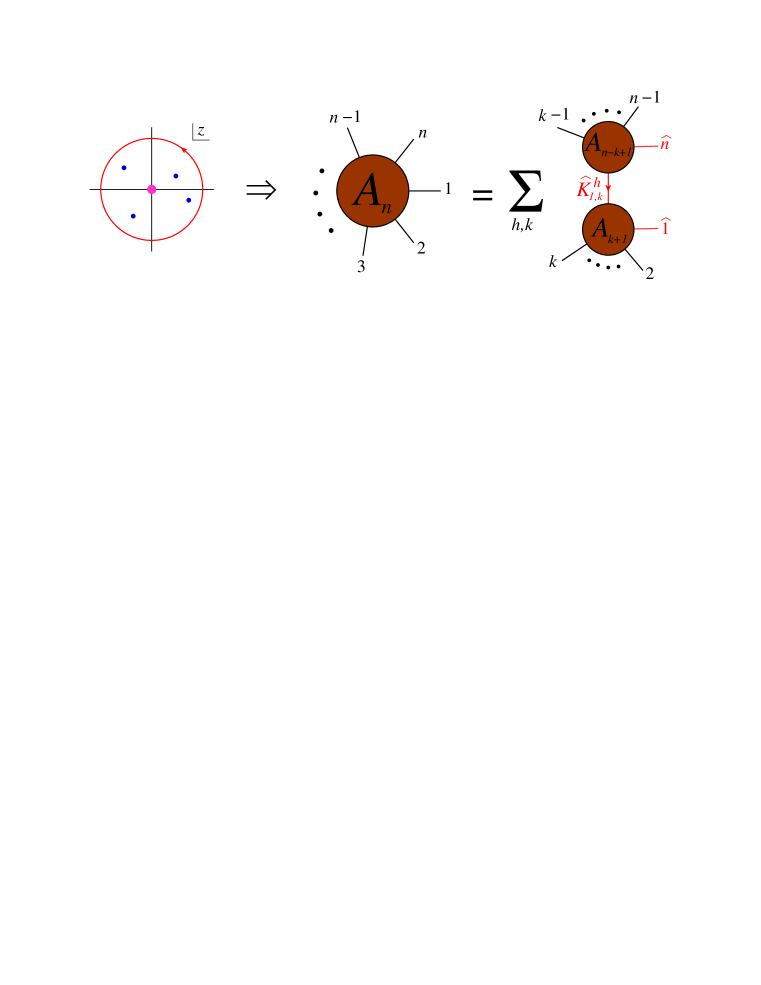
Figure 8: Illustration of how Cauchy’s theorem leads to the BCFW recursion relation. The magenta dot represents the residue at the origin; the blue dots the residues at $z_{k}$. In the recursion relation, the red lines carry complex, shifted momenta.

We also have to compute the residue of $A(z)/z$ at $z=z_{k}$. To do that we use eq. (69), which also holds for three-point factorizations in complex kinematics. The singular factor in the denominator that produces the residue is

$$zP^{2}(z)=z\hat{K}^{2}_{1,k}(z)\approx z_{k}\left\langle\smash{n}{\vphantom{1}}^{-}\right|{\not{\hbox{\kern-2.3pt$K$}}_{1,k}}\left|\smash{1}{\vphantom{1}}^{-}\right\rangle(z-z_{k})\approx-K_{1,k}^{2}\,(z-z_{k}).$$ (83)

Thus after taking the residue it contributes a factor of the corresponding scalar propagator, $i/K_{1,k}^{2}$, evaluated for the original unshifted kinematics where it is nonsingular.

Solving eq. (80) for $A_{n}(0)$ then gives the final BCFW formula [25],

$$A_{n}(1,2,\ldots,n)=\sum_{h=\pm}\sum_{k=2}^{n-2}A_{k+1}(\hat{1},2,\ldots,k,-\hat{K}_{1,k}^{-h})\frac{i}{K_{1,k}^{2}}A_{n-k+1}(\hat{K}_{1,k}^{h},k+1,k+2,\ldots,n-1,\hat{n}),$$ (84)

where the hat in the $k^{\rm th}$ term indicates that the shifted momentum is to be evaluated for $z=z_{k}$, and $h=\pm$ labels the sign of the helicity of the intermediate state carrying (complex) momentum $\hat{K}_{1,k}$. The sum is over the $n-3$ ordered partitions of the $n$ momenta into two sets, with at least a three-point amplitude on the left ($k\geq 2$) and also on the right ($k\leq n-2$). The recursion relation is depicted in fig. 8.

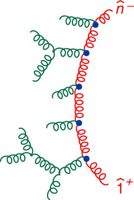
Figure 9: Large $z$ dependence of a generic Feynman diagram, for the $[n^{-},1^{+}\rangle$ momentum shift. Only the red gluons carry the large momentum.

In order to finish the proof of eq. (84), we need to show that $A_{n}(z)$ vanishes as $z\rightarrow\infty$. We will do so for the case that leg $n$ has negative helicity and leg $1$ has positive helicity, the so-called $[-,+\rangle$ case. This case can be demonstrated using Feynman diagrams [25]. The cases $[+,+\rangle$ and $[-,-\rangle$ also vanish at infinity, but the proof is slightly more involved. The case $[+,-\rangle$ diverges at infinity, so it should not be used as the basis for a recursion relation. Consider the large $z$ behavior of the generic Feynman diagram shown in fig. 9. Only the red gluons carry the large momentum proportional to $zv^{\mu}$. The red propagators contribute factors of the form

$$\frac{1}{\hat{K}_{1,k}^{2}(z)}=\frac{1}{K_{1,k}^{2}+z\left\langle\smash{n}{\vphantom{1}}^{-}\right|{\not{\hbox{\kern-2.3pt$K$}}_{1,k}}\left|\smash{1}{\vphantom{1}}^{-}\right\rangle}\sim\frac{1}{z}\,,\qquad\hbox{as }z\rightarrow\infty.$$ (85)

Yang-Mills vertices are (at worst) linear in the momentum, so they contribute a factor of $z$ per vertex. There is one more vertex than propagator, so the amplitude scales like $z^{+1}$ before we take into account the external polarization vectors. For the $[-,+\rangle$ case, they scale like,

$$\not{\hbox{\kern-2.3pt$\varepsilon$}}_{n}^{-}(q)\propto\frac{\lambda_{n}\tilde{\lambda}_{q}}{\left[n\,q\right]}\propto\frac{1}{z}\,,\qquad\not{\hbox{\kern-2.3pt$\varepsilon$}}_{1}^{+}(q)\propto\frac{\tilde{\lambda}_{1}\lambda_{q}}{\left\langle 1\,q\right\rangle}\propto\frac{1}{z}\,.$$ (86)

The two factors of $1/z$, combined with the factor of $z$ from the internal part of the diagram, mean that every Feynman diagram falls off like $1/z$, so $A_{n}(\infty)=0$ for the $[-,+\rangle$ shift.

It is easy to see that flipping either helicity in eq. (86) results in a polarization vector that scales like $z$ instead of $1/z$, invalidating the argument based on Feynman diagrams. However, it is possible to show [26] using the background field method that the $[+,+\rangle$ and $[-,-\rangle$ cases are actually just as well behaved as the $[-,+\rangle$ case, also falling off like $1/z$. In contrast, the $[+,-\rangle$ case does diverge like $z^{3}$, as suggested by the above diagrammatic argument.

5.2 Application to MHV

Next we apply the BCFW recursion relation to prove the form of the Parke-Taylor amplitudes (68), inductively in the number of legs $n$. For convenience, we will use cyclicity to put one of the two negative helicities in the $n^{\rm th}$ position,

$$A_{jn}^{\rm MHV}\ \equiv\ A_{n}^{\rm tree}(1^{+},2^{+},\ldots,j^{-},\ldots,(n-1)^{+},n^{-})\ =\ i\,\frac{{\left\langle j\,n\right\rangle}^{4}}{\left\langle 1\,2\right\rangle\cdots\left\langle n\,1\right\rangle}\,.$$ (87)

First we note that the middle terms in the sum over $k$ in eq. (84), with $3\leq k\leq n-3$ all vanish. That’s because they correspond to the multi-particle pole factorizations considered in eq. (69), with at least a four-point amplitude on each side of the factorization pole, and vanish according to the discussion below eq. (69), by counting negative helicities.

The case $k=n-2$ also vanishes. If $j=n-1$, then it vanishes because $A_{k+1}$ can have at most one negative helicity. If $j<n-1$, then we must have $h=+$ so that $A_{k+1}$ is non-vanishing, and then the three-point amplitude $A_{n-k+1}$ is of type $(+,+,-)$. This amplitude, given in eq. (75), can be nonvanishing when the three right-handed spinors $\lambda_{i}$ ($i=K,n-1,n$) are proportional (the second choice of three-point kinematics). However, we have shifted the left-handed spinor $\tilde{\lambda}_{n}$, not the right-handed one, and it is easy to check that the three-point configuration we arrived at is the one for which three left-handed spinors $\tilde{\lambda}_{i}$ are proportional. For this choice $A_{n-k+1}$ vanishes.

The only nonvanishing contribution is from $k=2$. We assume $j>2$ for simplicity. Since we have shifted $\lambda_{1}$, the three right-handed spinors $\lambda_{i}$ ($i=K,1,2$) must be proportional, which allows the following three-point amplitude to be non-vanishing:

$$A_{3}(\hat{1}^{+},2^{+},-\hat{K}^{-})=-i\frac{{\left[\hat{1}\,2\right]}^{4}}{[\hat{1}\,2][2\,(-\hat{K})][(-\hat{K})\,\hat{1}]}=+i\frac{{\left[1\,2\right]}^{3}}{[2\,\hat{K}][\hat{K}\,1]}\,,$$ (88)

where $\hat{K}=\hat{K}_{1,2}$. We removed the hats on 1 in the second step, since $\tilde{\lambda}_{1}$ is not shifted. There are also two factors of $i$ from reversing the sign of $\hat{K}$ in the spinor products.

The other amplitude appearing in the $k=2$ term in eq. (84) is evaluated using induction on $n$ and eq. (87):

$$A_{n-1}(\hat{K}^{+},3^{+},\ldots,j^{-},\ldots,n^{-}) = i\,\frac{{\left\langle j\,\hat{n}\right\rangle}^{4}}{\langle\hat{K}\,3\rangle\left\langle 3\,4\right\rangle\cdots\left\langle n-1,\,\hat{n}\right\rangle\langle\hat{n}\,\hat{K}\rangle}$$ (89)

$$= i\,\frac{{\left\langle j\,n\right\rangle}^{4}}{\langle\hat{K}\,3\rangle\left\langle 3\,4\right\rangle\cdots\left\langle n-1,\,n\right\rangle\langle n\,\hat{K}\rangle}\,,$$

where we can again remove the hats on $n$ because $\lambda_{n}$ is unshifted.

Combining the three factors in the $k=2$ term in the BCFW formula (eq. (84)) gives

$$A_{jn}^{\rm MHV}=-i\frac{{\left\langle j\,n\right\rangle}^{4}}{\langle\hat{K}\,3\rangle\left\langle 3\,4\right\rangle\cdots\left\langle n-1,\,n\right\rangle\langle n\,\hat{K}\rangle}\frac{1}{s_{12}}\frac{{\left[1\,2\right]}^{3}}{[2\,\hat{K}][\hat{K}\,1]}\,.$$ (90)

One can combine the $\hat{K}$-containing factors into $\langle n\,\hat{K}\rangle[\hat{K}\,2]$ and $\langle 3\,\hat{K}\rangle[\hat{K}\,1]$. At this point, we would normally need the value of $z_{k}$ to proceed. From eq. (82), it is

$$z_{2}=-\frac{s_{12}}{\left\langle\smash{n}{\vphantom{1}}^{-}\right|{(1+2)}\left|\smash{1}{\vphantom{1}}^{-}\right\rangle}=-\frac{\left\langle 1\,2\right\rangle\left[2\,1\right]}{\left\langle n\,2\right\rangle\left[2\,1\right]}=-\frac{\left\langle 1\,2\right\rangle}{\left\langle n\,2\right\rangle}\,.$$ (91)

However, the evaluation of the $\hat{K}$-containing strings in this case, where

$$\hat{\not{\hbox{\kern-2.3pt$K$}}}=\hat{\not{\hbox{\kern-2.3pt$K$}}}_{1,2}(z_{2})=\not{\hbox{\kern-2.3pt$k$}}_{1}+\not{\hbox{\kern-2.3pt$k$}}_{2}+z_{2}\lambda_{n}\tilde{\lambda}_{1}\,,$$ (92)

does not actually require the value of $z_{2}$:

$$\langle n\,\hat{K}\rangle[\hat{K}\,2] = \left\langle\smash{n}{\vphantom{1}}^{-}\right|{(1+2)}\left|\smash{2}{\vphantom{1}}^{-}\right\rangle+z_{2}\left\langle n\,n\right\rangle\left[1\,2\right]=\left\langle n\,1\right\rangle\left[1\,2\right]\,,$$

$$\langle 3\,\hat{K}\rangle[\hat{K}\,1] = \left\langle\smash{3}{\vphantom{1}}^{-}\right|{(1+2)}\left|\smash{1}{\vphantom{1}}^{-}\right\rangle+z_{2}\left\langle 3\,n\right\rangle\left[1\,1\right]=\left\langle 3\,2\right\rangle\left[2\,1\right]\,.$$ (93)

Inserting these results into eq. (90) gives

$$A_{jn}^{\rm MHV} = -i\frac{{\left\langle j\,n\right\rangle}^{4}{\left[1\,2\right]}^{3}}{(\left\langle 1\,2\right\rangle\left[2\,1\right])(\left[1\,2\right]\left\langle 2\,3\right\rangle)(\left\langle n\,1\right\rangle\left[1\,2\right])\left\langle 3\,4\right\rangle\cdots\left\langle n-1,\,n\right\rangle}$$ (94)

$$= i\frac{{\left\langle j\,n\right\rangle}^{4}}{\left\langle 1\,2\right\rangle\left\langle 2\,3\right\rangle\cdots\left\langle n-1,\,n\right\rangle\left\langle n\,1\right\rangle}\,,$$

completing the induction and proving the Parke-Taylor formula.

5.3 An NMHV application

Now we know all the MHV pure-gluon tree amplitudes with exactly two negative helicities, and by parity, all the $\overline{\rm MHV}$ amplitudes with exactly two positive helicities. The first gluonic amplitude which is not zero or one of these is encountered for six gluons, with three negative and three positive helicities, the next-to-MHV case. In fact, there are three inequivalent cases (up to cyclic permutations and reflection symmetries):

$$A_{6}(1^{+},2^{+},3^{+},4^{-},5^{-},6^{-}),\quad A_{6}(1^{+},2^{+},3^{-},4^{+},5^{-},6^{-}),\quad A_{6}(1^{+},2^{-},3^{+},4^{-},5^{+},6^{-}).$$ (95)

One can use a simple group theory relation known as the $U(1)$ decoupling identity to rewrite the third configuration in terms of the first two [15, 16].

Here we will give a final illustration of the BCFW recursion relation by computing the first of the amplitudes in eq. (95). (The other two are almost as simple to compute.) We again use the $[n^{-},1^{+}\rangle$ shift, for $n=6$. The $k=3$ term vanishes in this case because $A_{k+1}=A_{4}(\hat{1}^{+},2^{+},3^{+},-\hat{K}_{1,3}^{-h})=0$. The $k=2$ and $k=4$ terms are related by the following parity symmetry:

$$1\rangle\leftrightarrow 6],\quad 2\rangle\leftrightarrow 5],\quad 3\rangle\leftrightarrow 4],\quad 4\rangle\leftrightarrow 3],\quad 5\rangle\leftrightarrow 2],\quad 6\rangle\leftrightarrow 1].$$ (96)

For the $k=2$ term, using $z_{2}$ from eq. (91), we have the kinematical identities (where again $\hat{K}=\hat{K}_{1,2}$),

$$\hat{\not{\hbox{\kern-2.3pt$K$}}} = \not{\hbox{\kern-2.3pt$k$}}_{1}+\not{\hbox{\kern-2.3pt$k$}}_{2}-\frac{\left\langle 1\,2\right\rangle}{\left\langle 6\,2\right\rangle}|6\rangle[1|\,,$$ (97)

$$|\hat{1}] = |1]\,,$$ (98)

$$|\hat{6}] = |6]+\frac{\left\langle 1\,2\right\rangle}{\left\langle 6\,2\right\rangle}|1]\,.$$ (99)

The $k=2$ BCFW diagram is

$$T_{2} \equiv A_{3}(\hat{1}^{+},2^{+},-\hat{K}_{1,2}^{-})\frac{i}{s_{12}}A_{5}(\hat{K}_{1,2}^{+},3^{+},4^{-},5^{-},\hat{6}^{-})$$ (100)

$$= \frac{i}{s_{12}}\frac{{\left[\hat{1}\,2\right]}^{3}}{[2\,\hat{K}][\hat{K}\,1]}\frac{[\hat{K}\,3]^{3}}{\left[3\,4\right]\left[4\,5\right]\left[5\,\hat{6}\right][\hat{6}\,\hat{K}]}$$

$$= \frac{i}{s_{12}}\frac{{\left[1\,2\right]}^{3}}{([2\,\hat{K}]\langle\hat{K}\,6\rangle)(\langle 6\,\hat{K}\rangle[\hat{K}\,1])}\frac{(\langle 6\,\hat{K}\rangle[\hat{K}\,3])^{3}}{\left[3\,4\right]\left[4\,5\right]\left[5\,\hat{6}\right]([\hat{6}\,\hat{K}]\langle\hat{K}\,6\rangle)}\,.$$

Using eqs. (97) and (99), we can derive the identities,

$$\langle 6\,\hat{K}\rangle\bigl{[}\hat{K}\,a\bigr{]} = \left\langle\smash{6}{\vphantom{1}}^{-}\right|{(1+2)}\left|\smash{a}{\vphantom{1}}^{-}\right\rangle\,,$$

$$\left[5\,\hat{6}\right] = \left[5\,6\right]+\frac{\left\langle 1\,2\right\rangle\left[5\,1\right]}{\left\langle 6\,2\right\rangle}=\frac{\left\langle\smash{2}{\vphantom{1}}^{-}\right|{(6+1)}\left|\smash{5}{\vphantom{1}}^{-}\right\rangle}{\left\langle 6\,2\right\rangle}\,,$$

$$\bigl{[}\hat{6}\,\hat{K}\bigr{]}\langle\hat{K}\,6\rangle = \left\langle\smash{6}{\vphantom{1}}^{+}\right|{(1+2)}\left|\smash{6}{\vphantom{1}}^{+}\right\rangle+s_{12}=s_{612}\,,$$ (101)

where $s_{612}=(k_{6}+k_{1}+k_{2})^{2}$. Inserting these identities into eq. (100) for $T_{2}$, we have

$$T_{2}=i\,\frac{{\left\langle\smash{6}{\vphantom{1}}^{-}\right|{(1+2)}\left|\smash{3}{\vphantom{1}}^{-}\right\rangle}^{3}}{\left\langle 6\,1\right\rangle\left\langle 1\,2\right\rangle\left[3\,4\right]\left[4\,5\right]\,s_{612}\,\left\langle\smash{2}{\vphantom{1}}^{-}\right|{(6+1)}\left|\smash{5}{\vphantom{1}}^{-}\right\rangle}\,.$$ (102)

We can use the parity symmetry (96) to obtain the $k=4$ term. The final result for the six-point NMHV amplitude is,

$$A_{6}(1^{+},2^{+},3^{+},4^{-},5^{-},6^{-}) = i\,\frac{{\left\langle\smash{6}{\vphantom{1}}^{-}\right|{(1+2)}\left|\smash{3}{\vphantom{1}}^{-}\right\rangle}^{3}}{\left\langle 6\,1\right\rangle\left\langle 1\,2\right\rangle\left[3\,4\right]\left[4\,5\right]\,s_{612}\,\left\langle\smash{2}{\vphantom{1}}^{-}\right|{(6+1)}\left|\smash{5}{\vphantom{1}}^{-}\right\rangle}$$ (103)

$$\hskip-11.38092pt\hbox{}+i\,\frac{{\left\langle\smash{4}{\vphantom{1}}^{-}\right|{(5+6)}\left|\smash{1}{\vphantom{1}}^{-}\right\rangle}^{3}}{\left\langle 2\,3\right\rangle\left\langle 3\,4\right\rangle\left[5\,6\right]\left[6\,1\right]\,s_{561}\,\left\langle\smash{2}{\vphantom{1}}^{-}\right|{(6+1)}\left|\smash{5}{\vphantom{1}}^{-}\right\rangle}\,.$$

It’s worth comparing the analytic form of this result to that found in the 1980’s [22],

$$A_{6}(1^{+},2^{+},3^{+},4^{-},5^{-},6^{-}) = i\,\frac{(\left[1\,2\right]\left\langle 4\,5\right\rangle\left\langle\smash{6}{\vphantom{1}}^{-}\right|{(1+2)}\left|\smash{3}{\vphantom{1}}^{-}\right\rangle)^{2}}{s_{61}s_{12}s_{34}s_{45}s_{612}}$$

$$\hskip-11.38092pt\hbox{}+i\,\frac{(\left[2\,3\right]\left\langle 5\,6\right\rangle\left\langle\smash{4}{\vphantom{1}}^{-}\right|{(2+3)}\left|\smash{1}{\vphantom{1}}^{-}\right\rangle)^{2}}{s_{23}s_{34}s_{56}s_{61}s_{561}}$$

$$\hskip-11.38092pt\hbox{}+i\,\frac{s_{123}\left[1\,2\right]\left[2\,3\right]\left\langle 4\,5\right\rangle\left\langle 5\,6\right\rangle\left\langle\smash{6}{\vphantom{1}}^{-}\right|{(1+2)}\left|\smash{3}{\vphantom{1}}^{-}\right\rangle\left\langle\smash{4}{\vphantom{1}}^{-}\right|{(2+3)}\left|\smash{1}{\vphantom{1}}^{-}\right\rangle}{s_{12}s_{23}s_{34}s_{45}s_{56}s_{61}}\,.$$

Although the new form has only one fewer term, it represents the physical singularities in a cleaner fashion. For example, in the collinear limit $3\parallel 4$, eq. (103) makes manifest the $1/\left\langle 3\,4\right\rangle$ and $1/\left[3\,4\right]$ singularities, which correspond to the two different intermediate gluon helicities that contribute in this collinear channel, as the six-point NMHV amplitude factorizes on both the MHV and $\overline{\rm MHV}$ five-point amplitudes, $A_{5}(1^{+},2^{+},P^{\pm},5^{-},6^{-})$. On the other hand, each term of eq. (5.3) behaves like the product of these two singularities, since $1/s_{3,4}=-1/(\left\langle 3\,4\right\rangle\left[3\,4\right])$. Hence there are large cancellations between the three terms in this channel. Such cancellations can lead to large losses in numerical precision due to round-off errors, especially in NLO calculations which typically evaluate tree amplitudes repeatedly close to the collinear poles.

On the other hand, eq. (103) contains a spurious singularity that eq. (5.3) does not, as $\left\langle\smash{2}{\vphantom{1}}^{-}\right|{(6+1)}\left|\smash{5}{\vphantom{1}}^{-}\right\rangle\rightarrow 0$. This can happen, for example, whenever $k_{6}+k_{1}$ is a linear combination of $k_{2}$ and $k_{5}$. (In the collision $2+5\rightarrow 6+1+3+4$, such a configuration is reached if the vectors $k_{6}+k_{1}$ and $k_{3}+k_{4}$ have no component transverse to the beam axis defined by $k_{2}$ and $k_{5}$; that is, if $k_{6}+k_{1}$ is a linear combintation of $k_{2}$ and $k_{5}$.) It’s called a spurious singularity because the amplitude should evaluate to a finite number there, but individual terms blow up. However, these singularities tend to have milder consequences, as long as they appear only to the first power, as they do here. That’s because the amplitude is not particularly large in this region, so in the evaluation of an integral containing it by importance-sampling, it is rare to come close enough to the surface where $\left\langle\smash{2}{\vphantom{1}}^{-}\right|{(6+1)}\left|\smash{5}{\vphantom{1}}^{-}\right\rangle$ vanishes that round-off error is a problem. Different choices of BCFW shifts lead to different spurious singularities, so one can always check the value of $\left\langle\smash{2}{\vphantom{1}}^{-}\right|{(6+1)}\left|\smash{5}{\vphantom{1}}^{-}\right\rangle$ and use a different shift if it is too small.

In general, the BCFW recursion relation leads to very compact analytic representations for tree amplitudes. The relative simplicity with respect to previous analytic approaches becomes much more striking for seven or more external legs. A closely related set of recursion relations for ${\cal N}=4$ super-Yang-Mills theory [27] have been solved in closed form for an arbitrary number of external legs [28]. These solutions can also be used to compute efficiently a wide variety of QCD tree amplitudes [29]. There are other ways to compute tree amplitudes, in particular, off-shell recursion relations based on the Dyson-Schwinger equations, such as the Berends-Giele recursion relations [6]. At very high multiplicities, these can be numerically even more efficient than the BCFW recursion relations. Nevertheless, the idea behind the BCFW recursion relations, that amplitudes can be reconstructed from their analytic behavior, carries over to the loop level, as we’ll now discuss.

6 Generalized unitarity and loop amplitudes

Ordinary unitarity is merely the statement that the scattering matrix $S$ is a unitary matrix, $S^{\dagger}S=1$. Usually we split off a forward-scattering part by writing $S=1+iT$, leading to $(1-iT^{\dagger})(1+iT)=1$, or

$${\rm Disc}\,T=T^{\dagger}T\,,$$ (105)

where ${\rm Disc}(x)=2\,{\rm Im}(x)$ is the discontinuity across a branch cut. This equation can be expanded order-by-order in perturbation theory. For example, the four- and five-gluon scattering amplitudes in QCD have the expansions,

$$T_{4} = g^{2}T_{4}^{(0)}+g^{4}T_{4}^{(1)}+g^{6}T_{4}^{(2)}+\ldots,$$ (106)

$$T_{5} = g^{3}T_{5}^{(0)}+g^{5}T_{5}^{(1)}+g^{7}T_{5}^{(2)}+\ldots,$$ (107)

where $T_{n}^{(L)}$ is the $L$-loop $n$-gluon amplitude. Inserting these expansions into eq. (105) for the four-point amplitude and collecting the coefficients at order $g^{2}$, $g^{4}$ and $g^{6}$, respectively, we find that,

$${\rm Disc}\,T_{4}^{(0)} = 0\,,$$ (108)

$${\rm Disc}\,T_{4}^{(1)} = T_{4}^{(0)\,\dagger}T_{4}^{(0)}\,,$$ (109)

$${\rm Disc}\,T_{4}^{(2)} = T_{4}^{(0)\,\dagger}T_{4}^{(1)}+T_{4}^{(1)\,\dagger}T_{4}^{(0)}+T_{5}^{(0)\,\dagger}T_{5}^{(0)}\,.$$ (110)

On the right-hand sides of these equations, there is an implicit discrete sum over the types and helicities of the intermediate states which lie between the two $T$ matrices, and there is a continuous integral over the intermediate-state phase space.

The first equation (generalized to more legs) simply states that tree amplitudes have no branch cuts. The second equation, eq. (109), states that the discontinuities of one-loop amplitudes are given by the products of tree amplitudes, where the intermediate state always consists of two particles that are re-scattering, the so-called two-particle cuts. The third equation, eq. (110), states that the discontinuities of two-loop amplitudes are of two types: two-particle cuts where one of the two amplitudes is a one-loop amplitude rather than a tree amplitude, and three-particle cuts involving the product of higher-multiplicity tree amplitudes.

Although there is a lot of information in eqs. (109) and (110), there are two more observations which lead to even more powerful conclusions. The first observation is that the above unitarity relations are derived assuming real momenta (and positive energies) for both the external states and the intermediate states appearing on the right-hand sides. The intermediate momenta on the right-hand sides can be thought of as particular values of the loop momenta implicit on the left-hand side, momenta that are real and on the particles’ mass shell. Given what we have learned so far about the utility of complex momenta at tree level, it is natural to try to solve the on-shell conditions for the loop momenta for complex momenta as well. Such solutions are referred to as generalized unitarity [30].

Secondly, because unitarity is being applied perturbatively, we might as well make use of other the properties of perturbation theory, namely that a Feynman diagram expansion exists. We don’t need to use the actual values of the Feynman diagrams, but it is very useful to know that such an expansion exists, because we can represent the loop amplitudes as a linear combination of a basic set of Feynman integrals, called master integrals, multiplied by coefficient functions. The idea of the unitarity method [9] is that the information from (generalized) unitarity cuts can be compared with the cuts of this linear combination, in order to determine all of the coefficient functions. If all possible integral coefficients can be determined, then the amplitude itself is completely determined. This approach avoids the need to use dispersion relations to reconstruct full amplitudes from their branch cuts, which is often necessary in the absence of a perturbative expansion.

In the rest of this section, we will sketch a useful hierarchical procedure for determining one-loop amplitudes from generalized unitarity. This method, and variations of it, have been implemented both analytically, and even more powerfully, numerically. The latter implementation has made it possible to compute efficiently one-loop QCD amplitudes of very high multiplicity, far beyond what was imaginable a decade ago. The availability of such loop amplitudes has broken a bottleneck in NLO QCD computations, particularly for processes at hadron colliders such as the LHC, leading to the “NLO revolution.”

6.1 The plastic loop integrand

Before carrying out the loop integration, the integrand of a one-loop amplitude depends on the external momenta $k_{1},k_{2},\ldots,k_{n}$ and on the loop momentum $\ell$. Just as at tree level, this function can develop poles as the various momenta are continued analytically. Suppose we hold the external momenta fixed and just vary $\ell$. One kind of singularity that can appear is the ordinary two-particle cut represented by eq. (109). Let’s first generalize this equation to the case of an $n$-gluon one-loop amplitude, and specialize it to the case of a color-ordered loop amplitude $A_{n}^{\rm 1\!-\!loop}$ — the coefficient of the leading-color single-trace color structure discussed in section 2.

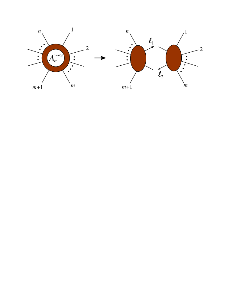
Figure 10: Ordinary unitarity viewed as a factorization property of the loop integrand.

Consider the discontinuity in the channel $s_{12\ldots m}=(k_{1}+k_{2}+\cdots k_{m})^{2}$, which is illustrated in fig. 10. The unitarity relation that generalizes eq. (109) is

$${\rm Disc}|_{s_{12\ldots m}}A_{n}^{\rm 1\!-\!loop}(k_{1},k_{2},\ldots,k_{n})$$ (112)

$$= (2\pi)^{2}\!\sum_{h_{i}}\int\frac{d^{D}\ell_{1}}{(2\pi)^{D}}\;\delta^{(+)}(\ell_{1}^{\mu})A_{m+2}^{\rm tree}(-\ell_{1}^{-h_{1}},k_{1},\ldots,k_{m},\ell_{2}^{h_{2}})\,,$$

$$\hskip 73.97733pt\hbox{}\times\delta^{(+)}(-\ell_{2}^{\mu})A_{n-m+2}^{\rm tree}(-\ell_{2}^{-h_{2}},k_{m+1},\ldots,k_{n},\ell_{1}^{h_{1}})$$

where $\ell_{2}=\ell_{1}-(k_{1}+k_{2}+\cdots k_{m})$. The delta function $\delta^{(+)}(k^{\mu})=\Theta(k^{0})\delta(k^{2})$ enforces that the intermediate states are on shell with real momenta and positive energies. The sum over intermediate helicities may also include different particle types, for example, both gluons and quarks in an $n$-gluon QCD loop amplitude. The two delta functions reduce the loop momentum integral to an integral over the two-body phase space for on-shell momenta $\ell_{1}$ and $-\ell_{2}$.

Another way of stating eq. (112), which allows us to generalize it, is that for a given set of external momenta $k_{i}$, there is a family of loop momenta $\ell\equiv\ell_{1}$ that solve the dual constraints $\ell_{1}^{2}=\ell_{2}^{2}=0$. On this solution set the loop integrand, which can be pictured as the annular blob shown in fig. 10, factorizes into the product of two tree amplitudes,

$$\frac{i}{\ell_{1}^{2}}A_{m+2}^{\rm tree}(-\ell_{1}^{-h_{1}},k_{1},\ldots,k_{m},\ell_{2}^{h_{2}})\frac{i}{\ell_{2}^{2}}A_{n-m+2}^{\rm tree}(-\ell_{2}^{-h_{2}},k_{m+1},\ldots,k_{n},\ell_{1}^{h_{1}})\,,$$ (113)

in much the same way that a tree amplitude factorizes on a single multi-particle pole, eq. (69).

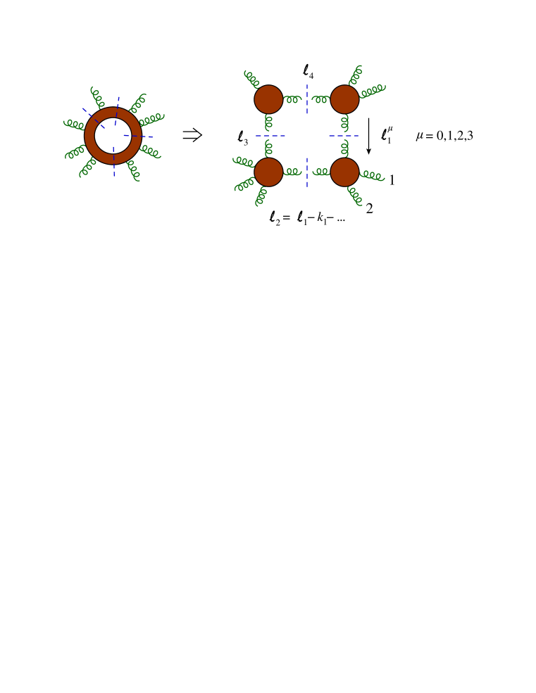
Figure 11: A quadruple cut pinches the loop integrand down into the product of four tree amplitudes, connected cyclicly around the loop.

In this picture of the plastic loop integrand, we need not impose positivity of the energies of the intermediate states, and the loop momenta can even be complex. This opens up the possibility of more general solutions, where more than two lines are cut. If we think of the loop momentum $\ell^{\mu}$ as four-dimensional, then for generic kinematics we can cut not just two lines, but up to four. The reason the maximum is four is that each cut imposes a new equation of the form $(\ell-K_{i})^{2}=0$ for some combination of external momenta $K_{i}$. At four cuts the number of equations equals the number of unknowns — the four components of $\ell^{\mu}$. Hence a fifth cut condition is impossible to satisfy (unless the kinematical configuration of the external momenta is an exceptional, degenerate one). Figure 11 shows how the quadruple cut of a generic one-loop integrand squeezes it at four locations, so that it becomes proportional to the product of four tree amplitudes. Two of the momenta of each tree amplitude are identified with the cut loop momenta, denoted by $\ell_{1},\ell_{2},\ell_{3},\ell_{4}$, and the rest are drawn from the external momenta for the loop amplitude.

6.2 The quadruple cut

The quadruple cut [31] is special because the solution set is discrete. Let’s write the four cut loop momenta as

$$\ell_{1},\qquad\ell_{2}=\ell_{1}-K_{1},\qquad\ell_{3}=\ell_{2}-K_{2},\qquad\ell_{4}=\ell_{3}-K_{3}=\ell_{1}+K_{4},$$ (114)

where the $K_{i}$ are sums of the $n$ external momenta satisfying $K_{1}+K_{2}+K_{3}+K_{4}=0$. From fig. 11 it is clear that the $K_{i}$ correspond to some partition of the $n$ cyclicly ordered momenta into four contiguous sets. We can rewrite the four quadratic cut conditions,

$$\ell_{1}^{2}=\ell_{2}^{2}=\ell_{3}^{2}=\ell_{4}^{2}=0,$$ (115)

by taking the differences $\ell_{i}^{2}-\ell_{i+1}^{2}=0$, so that three of the conditions are linear,

$$\ell_{1}^{2}=0,\qquad 2\ell_{1}\cdot K_{1}=K_{1}^{2},\qquad 2\ell_{2}\cdot K_{2}=K_{2}^{2},\qquad 2\ell_{3}\cdot K_{3}=K_{3}^{2}.$$ (116)

Because the three linear equations can be solved uniquely, we generically expect two discrete solutions for the loop momentum $\ell_{1}$, denoted by $\ell_{1}^{\pm}$. The other three quantities $\ell_{i}^{\pm}$ are uniquely determined from $\ell_{1}^{\pm}$ by shifting it by the appropriate external momenta.

Figure 12: Decomposition of a generic one-loop amplitude $A_{n}^{\rm 1\!-\!loop}$ into basis integrals multiplied by kinematical coefficients: scalar box integrals with coefficients $d_{i}$, scalar triangles with coefficients $c_{i}$, scalar bubbles with coefficients $b_{i}$, and the rational part $R_{n}$. The dots between the external lines indicate that one or several external legs may emanate from each vertex. If there are massive internal propagators, then tadpole integrals also appear; in the massless case such integrals vanish.

What information does the quadruple cut reveal? To answer this question, we rely on a systematic decomposition of the one-loop amplitude for an arbitrary $n$-point amplitude, which is shown diagramatically in fig. 12. The amplitude can be written as a linear combination of certain basis integrals, multiplied by kinematical coefficients. The only loop integrals that appear are scalar integrals with four, three and two internal propagator lines, which are usually called box, triangle and bubble integrals, respectively. They are given in dimensional regularization, with $D=4-2\epsilon$, by

$${\cal I}_{4}(K_{1},K_{2},K_{3},K_{4}) = \mu^{2\epsilon}\int{d^{4-2\epsilon}\ell\over(2\pi)^{4-2\epsilon}}{1\over\ell^{2}(\ell-K_{1})^{2}(\ell-K_{1}-K_{2})^{2}(\ell+K_{4})^{2}}\,,$$ (117)

$${\cal I}_{3}(K_{1},K_{2},K_{3}) = \mu^{2\epsilon}\int{d^{4-2\epsilon}\ell\over(2\pi)^{4-2\epsilon}}{1\over\ell^{2}(\ell-K_{1})^{2}(\ell+K_{3})^{2}}\,,$$ (118)

$${\cal I}_{2}(K) = \mu^{2\epsilon}\int{d^{4-2\epsilon}\ell\over(2\pi)^{4-2\epsilon}}{1\over\ell^{2}(\ell-K)^{2}}\,,$$ (119)

where the $K_{i}$ are the sums of external momenta emanating from each corner. The coefficients of these integrals are $d_{i}$, $c_{i}$ and $b_{i}$, where $i$ labels all the inequivalent partitions of the $n$ external momenta into 4, 3 and 2 sets, respectively. There is also a rational part $R_{n}$, which cannot be detected using cuts with four-dimensional cut loop momenta; we will return to this contribution later.

The decomposition in fig. 12 holds in dimensional regularization, assuming that the external (observable) momenta are all four-dimensional, and neglecting the ${\cal O}(\epsilon)$ terms. It also requires the internal propagators to be massless; if there are internal propagators for massive particles, then tadpole (one-propagator) integrals will also appear. The result seems remarkable at first sight, since one-loop Feynman diagrams with five or more external legs attached to the loop will generically appear, and these diagrams would seem likely to generate pentagon and higher-point integrals. However, it is possible to systematically reduce such integrals down to linear combinations of scalar boxes, triangles and bubble integrals [32, 33, 34].

The reduction formulas are fairly technical, but here we don’t need to know the formulas, just that the reduction is possible. Heuristically, the reason it is possible to avoid all pentagon and higher-point integrals is the same reason that there is no quintuple cut when the loop momentum is in four dimensions: there are more equations in the quintuple cut conditions than there are unknowns. If the scalar pentagon integral had a quintuple cut, it would not be possible to reduce it to a linear combination of box integrals. The fact that it can be done [32] exploits the four-dimensionality of the loop momenta to expand the loop momenta in terms of the four linearly-independent external momenta of the pentagon. In dimensional regularization, the relation of ref. [32] has a correction term [33], and the pentagon integral has a quintuple cut, because the loop momentum is no longer four-dimensional. However, because of the “small” volume of the extra $-2\epsilon$ dimensions, the correction term is of ${\cal O}(\epsilon)$.

Returning to the quadruple cut, we see that a second special feature of it is that only one of the integrals in fig. 12 survives, for a given quadruple cut. First of all, none of the triangle and bubble terms can survive, because those integrals do not even have four propagators available to cut. There are many possible box integrals, for a large number of external legs, but each one box integral is in one-to-one correspondence with a different quadruple cut; both are characterized by the same partition of the cyclicly ordered momenta into four contiguous sets, or clusters. The momentum flowing out at each corner of the box must match the cluster momenta $\{K_{1},K_{2},K_{3},K_{4}\}$ corresponding to the quadruple cut (115). For this solution, we match the left- and right-hand sides of fig. 12 and learn [31] that

$$d_{i}=\frac{1}{2}\Bigl{(}d_{i}^{+}+d_{i}^{-}\Bigr{)},$$ (120)

where the superscripts $\pm$ refer to the two discrete solutions for the loop momentum, and $d_{i}^{\pm}$ are given by the product of four tree amplitudes, as in fig. 11,

$$d_{i}^{\pm}=A_{1}^{\rm tree}(\ell^{\pm})A_{2}^{\rm tree}(\ell^{\pm})A_{3}^{\rm tree}(\ell^{\pm})A_{4}^{\rm tree}(\ell^{\pm}),$$ (121)

with

$$A_{i}^{\rm tree}(\ell)\equiv A^{\rm tree}(-\ell_{i},k^{(i)}_{1},\ldots,k^{(i)}_{p_{i}},\ell_{i+1}).$$ (122)

Here the external momenta $\{k^{(i)}_{1},\ldots,k^{(i)}_{p_{i}}\}$ are the elements of the cluster $K_{i}$, $i=1,2,3,4$, i.e. $\sum_{j=1}^{p_{i}}k^{(i)}_{j}=K_{i}$. These formulae are very easy to evaluate, either analytically or in an automated code, and they are numerically very stable.

It’s possible to solve analytically for the cut loop momenta $\ell_{i}^{\pm}$ for generic values of the $K_{i}$; the solution involves a quadratic formula [31]. If just one of the external legs is massless, however, say $K_{1}=k_{1}$, then the solutions collapse to a simpler form [35, 36]:

$$(\ell_{1}^{\pm})^{\mu}={\left\langle\smash{1^{\mp}}\vphantom{1}\right|{{\raise 0.91666pt\hbox to9.20833pt{\hss/\hss}\hbox to0.0pt{\hss$K$}}_{2}{\raise 0.91666pt\hbox to9.20833pt{\hss/\hss}\hbox to0.0pt{\hss$K$}}_{3}{\raise 0.91666pt\hbox to9.20833pt{\hss/\hss}\hbox to0.0pt{\hss$K$}}_{4}\gamma^{\mu}}\left|\smash{1^{\pm}}{\vphantom{1}}\right\rangle\over 2\left\langle\smash{1^{\mp}}\vphantom{1}\right|{{\raise 0.91666pt\hbox to9.20833pt{\hss/\hss}\hbox to0.0pt{\hss$K$}}_{2}{\raise 0.91666pt\hbox to9.20833pt{\hss/\hss}\hbox to0.0pt{\hss$K$}}_{4}}\left|\smash{1^{\pm}}{\vphantom{1}}\right\rangle}\,,\hskip 56.9055pt(\ell_{2}^{\pm})^{\mu}=-{\left\langle\smash{1^{\mp}}\vphantom{1}\right|{\gamma^{\mu}{\raise 0.91666pt\hbox to9.20833pt{\hss/\hss}\hbox to0.0pt{\hss$K$}}_{2}{\raise 0.91666pt\hbox to9.20833pt{\hss/\hss}\hbox to0.0pt{\hss$K$}}_{3}{\raise 0.91666pt\hbox to9.20833pt{\hss/\hss}\hbox to0.0pt{\hss$K$}}_{4}}\left|\smash{1^{\pm}}{\vphantom{1}}\right\rangle\over 2\left\langle\smash{1^{\mp}}\vphantom{1}\right|{{\raise 0.91666pt\hbox to9.20833pt{\hss/\hss}\hbox to0.0pt{\hss$K$}}_{2}{\raise 0.91666pt\hbox to9.20833pt{\hss/\hss}\hbox to0.0pt{\hss$K$}}_{4}}\left|\smash{1^{\pm}}{\vphantom{1}}\right\rangle}\,,$$

$$(\ell_{3}^{\pm})^{\mu}={\left\langle\smash{1^{\mp}}\vphantom{1}\right|{{\raise 0.91666pt\hbox to9.20833pt{\hss/\hss}\hbox to0.0pt{\hss$K$}}_{2}\gamma^{\mu}{\raise 0.91666pt\hbox to9.20833pt{\hss/\hss}\hbox to0.0pt{\hss$K$}}_{3}{\raise 0.91666pt\hbox to9.20833pt{\hss/\hss}\hbox to0.0pt{\hss$K$}}_{4}}\left|\smash{1^{\pm}}{\vphantom{1}}\right\rangle\over 2\left\langle\smash{1^{\mp}}\vphantom{1}\right|{{\raise 0.91666pt\hbox to9.20833pt{\hss/\hss}\hbox to0.0pt{\hss$K$}}_{2}{\raise 0.91666pt\hbox to9.20833pt{\hss/\hss}\hbox to0.0pt{\hss$K$}}_{4}}\left|\smash{1^{\pm}}{\vphantom{1}}\right\rangle}\,,\hskip 56.9055pt(\ell_{4}^{\pm})^{\mu}=-{\left\langle\smash{1^{\mp}}\vphantom{1}\right|{{\raise 0.91666pt\hbox to9.20833pt{\hss/\hss}\hbox to0.0pt{\hss$K$}}_{2}{\raise 0.91666pt\hbox to9.20833pt{\hss/\hss}\hbox to0.0pt{\hss$K$}}_{3}\gamma^{\mu}{\raise 0.91666pt\hbox to9.20833pt{\hss/\hss}\hbox to0.0pt{\hss$K$}}_{4}}\left|\smash{1^{\pm}}{\vphantom{1}}\right\rangle\over 2\left\langle\smash{1^{\mp}}\vphantom{1}\right|{{\raise 0.91666pt\hbox to9.20833pt{\hss/\hss}\hbox to0.0pt{\hss$K$}}_{2}{\raise 0.91666pt\hbox to9.20833pt{\hss/\hss}\hbox to0.0pt{\hss$K$}}_{4}}\left|\smash{1^{\pm}}{\vphantom{1}}\right\rangle}\,.\hskip 28.45274pt$$ (123)

It’s easy to see that eq. (115) is satisfied by eq. (123); that is, each of the four vectors $(\ell_{i}^{\pm})^{\mu}$ squares to zero. For example, the evaluation of $(\ell_{1}^{\pm})^{\mu}(\ell_{1}^{\pm})_{\mu}$ proceeds using the Fierz identity and is proportional to $\left\langle 1\,1\right\rangle=0$. The corresponding algebra for $(\ell_{3}^{\pm})^{2}$ involves $\left\langle\smash{1^{\mp}}\vphantom{1}\right|{{\raise 0.91666pt\hbox to9.20833pt{\hss/\hss}\hbox to0.0pt{\hss$K$}}_{2}{\raise 0.91666pt\hbox to9.20833pt{\hss/\hss}\hbox to0.0pt{\hss$K$}}_{2}}\left|\smash{1^{\pm}}{\vphantom{1}}\right\rangle=K_{2}^{2}\left\langle 1\,1\right\rangle=0$.

We also have to show that momentum conservation is satisfied, namely,

$$\ell_{2}-\ell_{3}=K_{2}\,,\qquad\ell_{3}-\ell_{4}=K_{3}\,,\qquad\ell_{4}-\ell_{1}=K_{4}\,.$$ (124)

The first equation is

$$(\ell_{2}^{\pm}-\ell_{3}^{\pm})^{\mu}=-{\left\langle\smash{1^{\mp}}\vphantom{1}\right|{\{\gamma^{\mu},{\raise 0.91666pt\hbox to9.20833pt{\hss/\hss}\hbox to0.0pt{\hss$K$}}_{2}\}{\raise 0.91666pt\hbox to9.20833pt{\hss/\hss}\hbox to0.0pt{\hss$K$}}_{3}{\raise 0.91666pt\hbox to9.20833pt{\hss/\hss}\hbox to0.0pt{\hss$K$}}_{4}}\left|\smash{1^{\pm}}{\vphantom{1}}\right\rangle\over 2\left\langle\smash{1^{\mp}}\vphantom{1}\right|{{\raise 0.91666pt\hbox to9.20833pt{\hss/\hss}\hbox to0.0pt{\hss$K$}}_{2}{\raise 0.91666pt\hbox to9.20833pt{\hss/\hss}\hbox to0.0pt{\hss$K$}}_{4}}\left|\smash{1^{\pm}}{\vphantom{1}}\right\rangle}=-K_{2}^{\mu}{\left\langle\smash{1^{\mp}}\vphantom{1}\right|{(-{\raise 0.97221pt\hbox to5.52084pt{\hss/\hss}\hbox to0.0pt{\hss$k$}}_{1}-{\raise 0.91666pt\hbox to9.20833pt{\hss/\hss}\hbox to0.0pt{\hss$K$}}_{2}-{\raise 0.91666pt\hbox to9.20833pt{\hss/\hss}\hbox to0.0pt{\hss$K$}}_{4}){\raise 0.91666pt\hbox to9.20833pt{\hss/\hss}\hbox to0.0pt{\hss$K$}}_{4}}\left|\smash{1^{\pm}}{\vphantom{1}}\right\rangle\over\left\langle\smash{1^{\mp}}\vphantom{1}\right|{{\raise 0.91666pt\hbox to9.20833pt{\hss/\hss}\hbox to0.0pt{\hss$K$}}_{2}{\raise 0.91666pt\hbox to9.20833pt{\hss/\hss}\hbox to0.0pt{\hss$K$}}_{4}}\left|\smash{1^{\pm}}{\vphantom{1}}\right\rangle}=K_{2}^{\mu}\,,$$ (125)

and the other equations work the same way.

Shortly, we will compute an explicit example of a nontrivial, nonzero coefficient of a box integral using the quadruple cut. However, it’s worth noting first that many box coefficients for massless QCD amplitudes vanish identically. In fact, the vanishing of large sets of box coefficients can be established simply by counting negative helicities. Consider, for example, the one-loop NMHV amplitude in massless QCD whose quadruple cut is shown on the left side of fig. 13. This quadruple cut can be used to compute the coefficient of a four-mass box integral. We call it a four-mass box because the momentum $K_{i}$ flowing out at each corner is the sum of at least two massless external particle momenta; hence $K_{i}$ is a massive four-vector. (In contrast, the right side of fig. 13 shows a quadruple cut for a three-mass box integral, because the lower right tree amplitude emits a single external momentum $m$.)

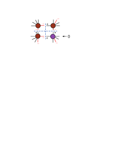
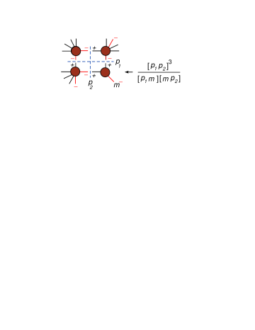
Figure 13: The left quadruple cut shows that the coefficients of all four-mass box integrals vanish for one-loop NMHV amplitudes. The right quadruple cut shows that the three-mass box coefficients do not vanish.

We denote negative-helicity legs by red lines and an explicit $(-)$ in the figure. The external black lines are all positive helicity. The upper left tree amplitude in the example has no external negative helicities. Because tree amplitudes with 0 or 1 negative helicity vanish, according to eq. (67), the two internal (cut) lines emanating from this upper left blob must carry negative helicity. On the opposite side of their respective cuts, they carry positive helicity. If the lower left and upper right tree amplitudes have one negative external helicity, as shown, then they must each send a negative helicity state toward the purple blob. This tree amplitude carries the third external negative helicity, but no other negative helicity emanates from it, so it vanishes, causing the vanishing of the corresponding four-mass box coefficient.

We gave this argument specifically for the case that all three negative-helicity particles were emitted from different corners of the box. It’s easy to see that the vanishing does not actually depend on where the negative helicities are located. It’s simply a reflection of the fact that there are four tree amplitudes, all with more than three legs, so there must be at least $4\times 2=8$ negative helicities among the external and cut legs. However, each cut has exactly one negative helicity, and there are three negative external helicities, for a total of $4+3=7$. Since $7<8$, the NMHV four-mass box coefficients always vanish. This counting argument fails as soon as one of the corner momenta becomes massless, as is appropriate for the three-mass cut shown on the right side of fig. 13. With the right (second) type of complex kinematics discussed in section 4.5, the three-point tree amplitude with helicity configuration $({+}{+}{-})$ is nonvanishing, as shown in the figure. Hence this three-mass box coefficient is nonvanishing. There is a single quadruple-cut helicity configuration and a single choice of sign for the kinematical configuration (123) that contributes in the particular case shown.

Using the same counting argument, we can see that one-loop MHV amplitudes, with two external negative helicities, contain neither four-mass, nor three-mass, box integrals. The two-mass box integrals can be divided into two types, “easy”, in which the two massive corners are diagonally opposite, and “hard”, in which they are adjacent to each other. One can show that the hard two-mass boxes always vanish as well. (This proof can be done with the help of a triple cut which puts the two massless corners into one of the three trees. Then the counting of negative helicities is analogous to the four-mass NMHV example, except that one needs $3\times 2=6$ negative helicities, and one has only $3+2=5$ available.)

As an aside, consider the one-loop amplitudes of the form $A_{n}^{\rm 1\!-\!loop}(1^{\pm},2^{+},\ldots,n^{+})$, for which the corresponding tree amplitudes vanished according to eq. (67). A similar counting exercise shows that they have no cuts at all: no quadruple, triple, or ordinary two-particle cuts. They are nonvanishing (at least in a non-supersymmetric theory like QCD), but they are forced to be purely rational functions of the external kinematics [37].

6.3 A five-point MHV box example

In the remainder of this section, we will compute one of the box coefficients for the five-gluon QCD amplitude $A_{5}^{\rm 1\!-\!loop}(1^{-},2^{-},3^{+},4^{+},5^{+})$, the one in which the two negative helicity legs, 1 and 2, are clustered into a massive leg (as also reviewed in ref. [10]). The quadruple cut for this box coefficient is shown in fig. 14. Inspecting the figure, starting with the lower-left tree amplitude, it is clear that there is a unique assignment of internal helicities. Also, this assignment of helicities forbids quarks (or scalars) from propagating in the loop; the tree amplitudes for two spin $1/2$ fermions (or two scalars) and two identical helicity gluons vanish (see eq. (71) for the fermion case). Therefore this box coefficient receives contributions only from the gluon loop, and is the same in QCD as in gauge theories with different matter content (such as ${\cal N}=4$ super-Yang-Mills theory).

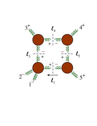
Figure 14: The quadruple cut for one of the box coefficients for the five-gluon amplitude with helicity configuration $({-}{-}{+}{+}{+})$.

Now that we have identified which four tree amplitudes are to be multiplied together, the next task is to determine the cut loop momentum. In particular, let’s work out $\ell_{4}$, the loop momentum just before the massless external leg 4. We can use eq. (123), but since leg 1 was massless there, we should relabel the momenta in that equation according to:

$$\ell_{1}^{\pm}\rightarrow\ell_{4}^{\pm}\,,\quad k_{1}\rightarrow k_{4}\,,\quad K_{2}\rightarrow k_{5}\,,\quad K_{3}\rightarrow k_{1}+k_{2}\,,\quad K_{4}\rightarrow k_{3}\,.$$ (126)

Then the first equation in (123) becomes,

$$(\ell_{4}^{\pm})^{\mu}={\left\langle\smash{4^{\mp}}\vphantom{1}\right|{5(1+2)3\gamma^{\mu}}\left|\smash{4^{\pm}}{\vphantom{1}}\right\rangle\over 2\left\langle\smash{4^{\mp}}\vphantom{1}\right|{53}\left|\smash{4^{\pm}}{\vphantom{1}}\right\rangle}=-{\left\langle\smash{4^{\mp}}\vphantom{1}\right|{543\gamma^{\mu}}\left|\smash{4^{\pm}}{\vphantom{1}}\right\rangle\over 2\left\langle\smash{4^{\mp}}\vphantom{1}\right|{53}\left|\smash{4^{\pm}}{\vphantom{1}}\right\rangle}=-{\left\langle\smash{5^{\pm}}\vphantom{1}\right|{43\gamma^{\mu}}\left|\smash{4^{\pm}}{\vphantom{1}}\right\rangle\over 2\left\langle\smash{5^{\pm}}\vphantom{1}\right|{3}\left|\smash{4^{\pm}}{\vphantom{1}}\right\rangle}\,.$$ (127)

Which sign should we use? The sign is dictated by the helicity assignments in the three-point amplitudes. Because the upper-right tree is of type $({-}{-}{+})$, and is constructed from right-handed spinors, the three left-handed spinors should be proportional. In particular, $\tilde{\lambda}_{\ell_{4}}\propto\tilde{\lambda}_{4}$, which tells us that we should take the lower sign in eq. (127), so that

$$\ell_{4}^{\mu}=(\ell_{4}^{-})^{\mu}=\frac{1}{2}\frac{\left\langle 4\,5\right\rangle}{\left\langle 3\,5\right\rangle}\left\langle\smash{3}{\vphantom{1}}^{-}\right|{\gamma^{\mu}}\left|\smash{4}{\vphantom{1}}^{-}\right\rangle\,.$$ (128)

Now we can multiply together the four tree amplitudes, and use eqs. (120) and (121) (with $d_{i}^{+}=0$) to get for the “$(12)$” box coefficient,

$$d_{(12)} = \frac{1}{2}A_{4}^{\rm tree}(-\ell_{1}^{+},1^{-},2^{-},\ell_{3}^{+})A_{3}^{\rm tree}(-\ell_{3}^{-},3^{+},\ell_{4}^{+})A_{3}^{\rm tree}(-\ell_{4}^{-},4^{+},\ell_{5}^{-})A_{3}^{\rm tree}(-\ell_{5}^{+},5^{+},\ell_{1}^{-})$$ (129)

$$= \frac{1}{2}\frac{\left\langle 1\,2\right\rangle^{3}}{\left\langle 2\,\ell_{3}\right\rangle\left\langle\ell_{3}\,(-\ell_{1})\right\rangle\left\langle(-\ell_{1})\,1\right\rangle}\frac{\left[3\,\ell_{4}\right]^{3}}{\left[\ell_{4}\,(-\ell_{3})\right]\left[(-\ell_{3})\,3\right]}\frac{\left\langle\ell_{5}\,(-\ell_{4})\right\rangle^{3}}{\left\langle 4\,\ell_{5}\right\rangle\left\langle(-\ell_{4})\,4\right\rangle}\frac{\left[(-\ell_{5})\,5\right]^{3}}{\left[5\,\ell_{1}\right]\left[\ell_{1}\,(-\ell_{5})\right]}$$

$$= -\frac{1}{2}\frac{\left\langle 1\,2\right\rangle^{3}\left\langle\smash{3}{\vphantom{1}}^{+}\right|{\ell_{4}\ell_{5}}\left|\smash{5}{\vphantom{1}}^{-}\right\rangle^{3}}{\left\langle\smash{2}{\vphantom{1}}^{-}\right|{\ell_{3}}\left|\smash{3}{\vphantom{1}}^{-}\right\rangle\left\langle\smash{4}{\vphantom{1}}^{-}\right|{\ell_{4}\ell_{3}\ell_{1}}\left|\smash{5}{\vphantom{1}}^{-}\right\rangle\left\langle\smash{1}{\vphantom{1}}^{-}\right|{\ell_{1}\ell_{5}}\left|\smash{4}{\vphantom{1}}^{+}\right\rangle}\,.$$

To get to the last step in eq. (129), we combined spinor products into longer strings using the replacement $|\ell_{i}\rangle[\ell_{i}|\rightarrow{\raise 0.04889pt\hbox to6.09596pt{\hss/\hss}\hbox to0.0pt{\hss$\ell_{i}$}}$, but we did not need to use any other properties of the $\ell_{i}$. In the next step it is convenient to use momentum conservation, i.e. $\ell_{1}=\ell_{4}-k_{4}-k_{5}$, $\ell_{3}=\ell_{4}+k_{3}$ and $\ell_{5}=\ell_{4}-k_{4}$, as well as $\ell_{i}^{2}=0$, to replace,

$$\left\langle\smash{3}{\vphantom{1}}^{+}\right|{\ell_{4}\ell_{5}}\left|\smash{5}{\vphantom{1}}^{-}\right\rangle \rightarrow -\left\langle\smash{4}{\vphantom{1}}^{-}\right|{\ell_{4}}\left|\smash{3}{\vphantom{1}}^{-}\right\rangle\left\langle 4\,5\right\rangle\,,$$ (130)

$$\left\langle\smash{2}{\vphantom{1}}^{-}\right|{\ell_{3}}\left|\smash{3}{\vphantom{1}}^{-}\right\rangle \rightarrow \left\langle\smash{2}{\vphantom{1}}^{-}\right|{\ell_{4}}\left|\smash{3}{\vphantom{1}}^{-}\right\rangle\,,$$ (131)

$$\left\langle\smash{4}{\vphantom{1}}^{-}\right|{\ell_{4}\ell_{3}\ell_{1}}\left|\smash{5}{\vphantom{1}}^{-}\right\rangle \rightarrow \left\langle\smash{4}{\vphantom{1}}^{-}\right|{\ell_{4}3(\ell_{4}-k_{4})}\left|\smash{5}{\vphantom{1}}^{-}\right\rangle=-\left\langle\smash{4}{\vphantom{1}}^{-}\right|{\ell_{4}}\left|\smash{3}{\vphantom{1}}^{-}\right\rangle\left\langle 3\,4\right\rangle\left[4\,5\right]\,,$$ (132)

$$\left\langle\smash{1}{\vphantom{1}}^{-}\right|{\ell_{1}\ell_{5}}\left|\smash{4}{\vphantom{1}}^{+}\right\rangle \rightarrow -\left\langle 1\,5\right\rangle\left\langle\smash{4}{\vphantom{1}}^{-}\right|{\ell_{4}}\left|\smash{5}{\vphantom{1}}^{-}\right\rangle\,.$$ (133)

In eq. (132) we also used the fact that $\left\langle 3\,\ell_{4}\right\rangle=0$, given that both $\ell_{4}$ and $k_{3}$ emanate from a $({+}{+}{-})$ three-point amplitude.

Making these replacements in eq. (129), and then Fierzing in $\ell_{4}^{\mu}\propto\left\langle\smash{3}{\vphantom{1}}^{-}\right|{\gamma^{\mu}}\left|\smash{4}{\vphantom{1}}^{-}\right\rangle$ from eq. (128), gives,

$$d_{(12)} = \frac{1}{2}\frac{\left\langle 1\,2\right\rangle^{3}\left\langle\smash{4}{\vphantom{1}}^{-}\right|{\ell_{4}}\left|\smash{3}{\vphantom{1}}^{-}\right\rangle^{2}\left[4\,5\right]^{3}}{\left\langle\smash{2}{\vphantom{1}}^{-}\right|{\ell_{4}}\left|\smash{3}{\vphantom{1}}^{-}\right\rangle\left\langle 3\,4\right\rangle\left[4\,5\right]\left\langle 1\,5\right\rangle\left\langle\smash{4}{\vphantom{1}}^{-}\right|{\ell_{4}}\left|\smash{5}{\vphantom{1}}^{-}\right\rangle}$$ (134)

$$= -\frac{1}{2}\frac{\left\langle 1\,2\right\rangle^{3}s_{34}s_{45}}{\left\langle 2\,3\right\rangle\left\langle 3\,4\right\rangle\left\langle 4\,5\right\rangle\left\langle 5\,1\right\rangle}$$

$$= \frac{i}{2}s_{34}s_{45}\,A_{5}^{\rm tree}(1^{-},2^{-},3^{+},4^{+},5^{+})\,.$$

For completeness, we give the formula for the one-mass box integral multiplying this coefficient. It is defined in eq. (117) and has the Laurent expansion in $\epsilon$,

$${\cal I}_{4}^{(12)} = {-2i\,c_{\Gamma}\over s_{34}s_{45}}\biggl{\{}-{1\over\epsilon^{2}}\biggl{[}\biggl{(}{\mu^{2}\over-s_{34}}\biggr{)}^{\epsilon}+\biggl{(}{\mu^{2}\over-s_{45}}\biggr{)}^{\epsilon}-\biggl{(}{\mu^{2}\over-s_{12}}\biggr{)}^{\epsilon}\biggr{]}$$ (135)

$$\hskip 34.14322pt+\mathop{\rm Li}\nolimits_{2}\biggl{(}1-{s_{12}\over s_{34}}\biggr{)}+\mathop{\rm Li}\nolimits_{2}\biggl{(}1-{s_{12}\over s_{45}}\biggr{)}+{1\over 2}\ln^{2}\biggl{(}{-s_{34}\over-s_{45}}\biggr{)}+{\pi^{2}\over 6}\biggr{\}}$$

$$\hskip 0.0pt+\ {\cal O}(\epsilon)\,,$$

where the constant $c_{\Gamma}$ is defined by

$$c_{\Gamma}={1\over(4\pi)^{2-\epsilon}}{\Gamma(1+\epsilon)\Gamma^{2}(1-\epsilon)\over\Gamma(1-2\epsilon)}\,.$$ (136)

Interestingly, the result (134) is proportional to the tree amplitude. The coefficients of the four other box integrals (labeled $(23)$, $(34)$, $(45)$ and $(51)$) also have only gluonic contributions for this helicity choice, and their coefficients turn out to be given by cyclic permutations of eq. (134). Hence we have for the gluonic contribution to the one-loop amplitude,

$$\hskip-14.22636ptA_{5}^{\rm 1\!-\!loop}(1^{-},2^{-},3^{+},4^{+},5^{+}) = A_{5}^{\rm tree}(1^{-},2^{-},3^{+},4^{+},5^{+})\,c_{\Gamma}\,\biggl{\{}$$ (137)

$$\hskip 0.0pt-{1\over\epsilon^{2}}\biggl{[}\biggl{(}{\mu^{2}\over-s_{34}}\biggr{)}^{\epsilon}+\biggl{(}{\mu^{2}\over-s_{45}}\biggr{)}^{\epsilon}-\biggl{(}{\mu^{2}\over-s_{12}}\biggr{)}^{\epsilon}\biggr{]}$$

$$\hskip 0.0pt+\mathop{\rm Li}\nolimits_{2}\biggl{(}1-{s_{12}\over s_{34}}\biggr{)}+\mathop{\rm Li}\nolimits_{2}\biggl{(}1-{s_{12}\over s_{45}}\biggr{)}+{1\over 2}\ln^{2}\biggl{(}{-s_{34}\over-s_{45}}\biggr{)}+{\pi^{2}\over 6}$$

$$\hskip 0.0pt+\ \hbox{cyclic permutations}\biggr{\}}$$

$$\hskip 0.0pt+\ \hbox{triangles + bubbles + rational}.$$

If we were computing the amplitude in ${\cal N}=4$ super-Yang-Mills theory, we would be done at this point: One can show that the triangles, bubbles and rational parts all vanish in this theory [9]. In the case of QCD, there is more work to do. In the next subsection we sketch a method [38, 35] for determining the triangle coefficients.

6.4 Triangle coefficients

By analogy, we expect the triangle coefficients to be determined by the triple cut shown in fig. 15(a), and the bubble coefficients by the double cut shown in fig. 15(b). The solution to the three equations defining the triple cut,

$$\ell_{1}^{2}(t)=\ell_{2}^{2}(t)=\ell_{3}^{2}(t)=0,$$ (138)

depends on a single complex parameter $t$. However, the triple cut generically also receives contributions from the box integral terms in fig. 12. The box contributions have to be removed before identifying the coefficient of a given scalar triangle integral. Take any one of the three tree amplitudes in fig. 15(a), and imagine pinching that blob until it splits into two, exposing another loop propagator. This corner of the triple-cut phase space has the form of a box integral contribution. The pinching imposed a fourth cut condition, which has discrete solutions, so it must only occur at discrete values of $t$, say $t_{i}^{\sigma}$ where $i$ labels the different quadruple cuts that sit “above” the given triple cut, and $\sigma=\pm$ labels the two possible discrete solutions.

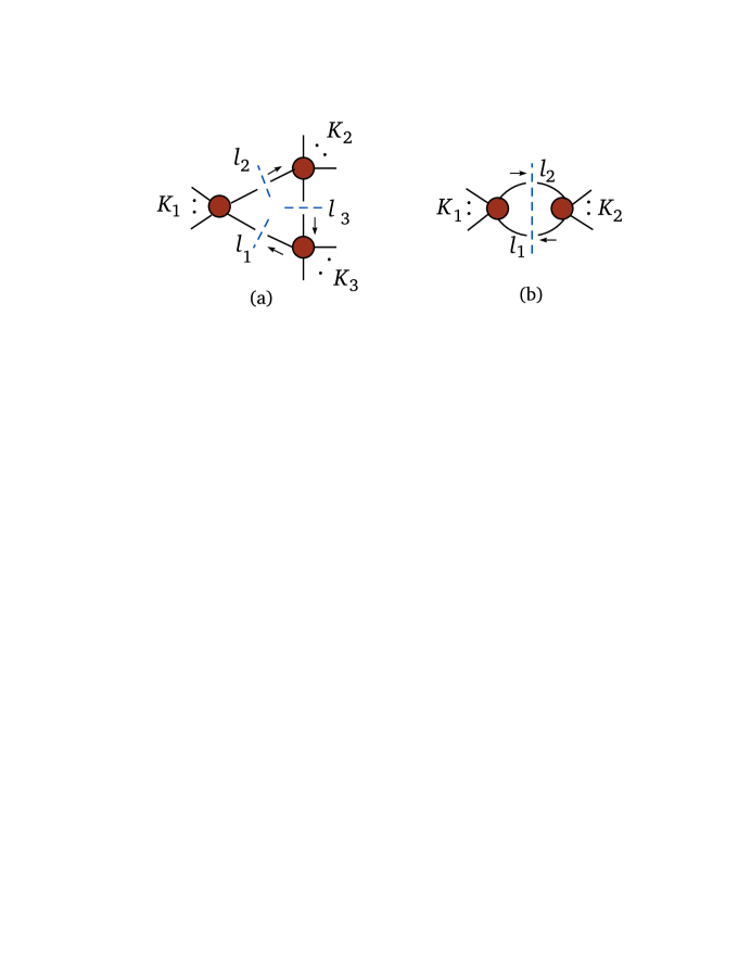
Figure 15: (a) The triple cut and (b) the ordinary double cut used to determine the coefficients of the triangle and bubble integrals. The loop momenta $l_{i}$ are constrained to satisfy on-shell conditions.

The generic form of the triple cut is

$$C_{3}(t) = A^{\rm tree}_{(1)}(-\ell_{1},k_{1},\ldots,k_{p_{1}},\ell_{2})A^{\rm tree}_{(2)}(-\ell_{2},k_{p_{1}+1},\ldots,k_{p_{2}},\ell_{3})A^{\rm tree}_{(3)}(-\ell_{3},k_{p_{2}+1},\ldots,k_{n},\ell_{1})$$ (139)

$$= T_{3}(t)+\sum_{\sigma=\pm}\sum_{i}\frac{d_{i}^{\sigma}}{\xi_{i}^{\sigma}(t-t_{i}^{\sigma})}\,,$$

where $d_{i}^{\sigma}$ are the previously computed box coefficients (121), and $T_{3}(t)$ is the triple cut “cleaned” of all singularities at finite $t$.

The pole locations $t_{i}^{\sigma}$ and the residue factors $\xi_{i}^{\sigma}$ do not depend on the amplitude being calculated, but only on the kinematics of the relevant triple and quadruple cuts. They can be computed from the solution for $\ell_{i}(t)$. For massless internal particles, the solution of eq. (138) is [39, 40, 38]

$$\ell^{\mu}_{1}(t)=\tilde{K}^{\mu}_{1}+\tilde{K}^{\mu}_{3}+\frac{t}{2}\langle\tilde{K}^{-}_{1}|\gamma^{\mu}|\tilde{K}^{-}_{3}\rangle+\frac{1}{2t}\langle\tilde{K}^{-}_{3}|\gamma^{\mu}|\tilde{K}^{-}_{1}\rangle\,,$$ (140)

and, using momentum conservation, $\ell_{2}(t)=\ell_{1}(t)-K_{1}$, $\ell_{3}(t)=\ell_{1}(t)+K_{3}$. Here we have introduced a pair of massless auxiliary vectors $\tilde{K}^{\mu}_{1}$ and $\tilde{K}^{\mu}_{3}$, constructed from $K_{1}$ and $K_{3}$,

$$\tilde{K}^{\mu}_{1}=\gamma\alpha\frac{\gamma K_{1}^{\mu}+S_{1}K^{\mu}_{3}}{\gamma^{2}-S_{1}S_{3}}\,,\hskip 56.9055pt\tilde{K}^{\mu}_{3}=-\gamma\alpha^{\prime}\frac{\gamma K_{3}^{\mu}+S_{3}K_{1}^{\mu}}{\gamma^{2}-S_{1}S_{3}}\,,$$ (141)

where $S_{1}=K_{1}^{2}$, $S_{3}=K_{3}^{2}$, and

$$\alpha=\frac{S_{3}(S_{1}-\gamma)}{S_{1}S_{3}-\gamma^{2}}\,,\qquad\alpha^{\prime}=\frac{S_{1}(S_{3}-\gamma)}{S_{1}S_{3}-\gamma^{2}}\,,\qquad\gamma=\gamma_{\pm}=-K_{1}\cdot K_{3}\pm\sqrt{\Delta}\,,$$ (142)

with

$$\Delta=(K_{1}\cdot K_{3})^{2}-K_{1}^{2}K_{3}^{2}\,.$$ (143)

The coefficient of the scalar triangle integral is the “$t$ independent” part of the triple cut. To be more precise, the quantity $T_{3}(t)$ has no singularities at finite values of $t$ because they are all accounted for by the box contributions shown explicitly in eq. (139). Because this quantity has singularities only at $t=0$ and $t=\infty$, it can be represented as,

$$T_{3}(t)=\sum_{k=-p}^{p}c_{k}t^{k}\,.$$ (144)

The desired quantity, the triangle coefficient, is $c_{0}$. The other terms correspond to tensor triangle integrals that integrate to zero (“spurious terms” in the language of OPP [40]). For renormalizable theories, there are at most three loop momenta in the numerator of triangle integrals, and one can take $p=3$.

One way to isolate $c_{0}$ is from the $t^{0}$ term in the large $t$ limit of $T_{3}(t)$, or of $C_{3}(t)$ itself, since the box contributions go to zero in this limit. This is an effective method for determining $c_{0}$ analytically [38]. For an automated implementation, the $t^{0}$ term is usually subleading as $t\rightarrow\infty$, making it difficult to extract numerically. Instead one can work at finite $t$, and extract $c_{0}$ (and the other $c_{k}$ coefficients) out of the finite sum in eq. (144) by using the discrete Fourier projection,

$$c_{k}={1\over 2p+1}\sum_{j=-p}^{p}\,\Bigl{[}t_{0}e^{2\pi ij/(2p+1)}\Bigr{]}^{-k}\,T_{3}\Bigl{(}t_{0}e^{2\pi ij/(2p+1)}\Bigr{)}\,,$$ (145)

for some choice of $t_{0}$. This approach is very stable numerically [35].

The other $c_{k}$ coefficients are actually needed in the next step, the determination of the bubble coefficients. The double cut depends on two complex parameters. It has singularities corresponding to both triple cuts and quadruple cuts, which can be “cleaned” in a fashion analogous to eq. (139), using the previously computed box and triangle information. Because the triple cut depends on a complex parameter, all of the $c_{k}$ coefficients are required to characterize it. After cleaning the double cut, a double discrete sum analogous to eq. (145) can be used to extract the bubble coefficient. For real cut momenta, the two parameters of the double cut have a simple physical interpretation: they are just the angles $\theta,\phi$ of one of the two intermediate states, in the center of mass frame for the channel being cut. The double discrete sum essentially performs a spherical harmonic expansion (it is slightly different because the intermediate momenta can be treated as complex).

The hierarchical determination of the “cut-constructible” parts of one-loop amplitudes described here [35] is quite similar to the OPP method [40] and to the method described in ref. [41], all of which have been implemented in an automated fashion.

6.5 The rational part

The last remaining part of the amplitude is the rational part $R_{n}$. This component cannot be detected by any unitarity cut in which the cut loop momentum are confined to four dimensions. We have implicitly been assuming throughout this section that the $\ell_{i}$ are four-dimensional. This assumption was very convenient because it allowed us to label the states with four-dimensional helicities, and use all the vanishing relations for the tree amplitudes that enter the four-dimensional cuts. One way to determine the rational part, called $D$-dimensional unitarity [42, 18, 43], is to let the cut momenta have extra-dimensional components, thinking of the $\epsilon$ in $D=4-2\epsilon$ as a negative number. In this approach, there are also nonvanishing quintuple cuts. There are no hexagon cuts because at one loop, all extra-dimensional components of the loop momentum are equivalent; they might as well point in a single, fifth dimension. So there are five components of the loop momentum that can be constrained by generalized cuts. The same kind of hierarchical, automated approach described above can be applied to the $D$-dimensional case [44]. In this case, one does not need to determine every extra-dimensional term in the loop integrand; the measure factor is $d^{-2\epsilon}\ell$, leading to an integral of ${\cal O}(\epsilon)$, unless there are enough factors of the extra-dimensional components, denoted by $\ell_{(-2\epsilon)}^{2}\equiv\mu^{2}$, in the numerator of the loop integrand to generate a compensating factor of $1/\epsilon$. For more details on this method, see the review [13].

A second method for computing the rational part is to apply a BCFW shift to the integrated loop amplitude. This approach can be implemented analytically [10], and numerically [35]. Here we just mention a few salient points. When a complex $z$-dependent shift is applied to a tree amplitude, as in section 5, the result is a meromorphic function of $z$, where the poles correspond to factorization of the tree amplitude into two lower-point amplitudes. When the same shift is applied to a loop amplitude, branch cuts in $z$ are generated, from the logarithms and dilogarithms appearing in the scalar integrals. There are also poles, whose origin from amplitude factorization is similar to the tree-level case. The branch cuts would complicate an analysis of the poles. However, if we have already computed the cut part $C_{n}$, we can consider shifting only the rational part, $R_{n}=A_{n}-C_{n}\rightarrow R_{n}(z)$.

The function $R_{n}(z)$ is meromorphic, so we can contemplate computing $R_{n}(0)$ from Cauchy’s theorem, using an equation analogous to eq. (80), if we know all of its poles and residues. However, $R_{n}(z)$ has two different types of poles. The physical poles are the ones that appear in $A_{n}(z)$, and their residues can be computed from factorization in a similar fashion to tree level. There is a second set of spurious poles. These poles are not poles of $A_{n}(z)$. They come from singularities in kinematical regions where $A_{n}$ is non-singular, but $C_{n}$ and $R_{n}$ separately diverge. (One example of such a region is where $\left\langle\smash{2}{\vphantom{1}}^{-}\right|{(6+1)}\left|\smash{5}{\vphantom{1}}^{-}\right\rangle\rightarrow 0$; see section 5.3.) Becasue $A_{n}(z)$ has no poles, the spurious-pole residues in $R_{n}(z)$ must be the negative those in $C_{n}(z)$. Because the cut part is known and the locations of all the spurious poles are known, the residues of $C_{n}(z)$ are straightforward to compute. For more details on this method, see the review [10].

Within the OPP method [40], the rational part is given by a sum of two terms, called $R_{1}$ and $R_{2}$. The $R_{1}$ part is obtained as a byproduct of the computation of the cut part, by taking into account the extra-dimensional $\mu^{2}$ dependence appearing in the propagator denominators of the dimensionally-regulated loop integrand [45]. The remaining $R_{2}$ terms come from $\mu^{2}$ dependence in the numerator of the loop integrand. As in the $D$-dimensional unitarity method, only a limited set of terms have enough factors of $\mu^{2}$ in the numerator to produce a nonzero rational term. For renormalizable theories, these contributions can be computed for all processes, in terms of a relatively small number of effective two-, three- and four-point vertices [45, 46].

These new, efficient methods have enabled the construction of a variety of automated computer programs for generating one-loop amplitudes, including CutTools [47], BlackHat [35], Rocket [48], SAMURAI [49], NGluon [50], MadLoop [51], HELAC-NLO [52], GoSam [53], Open Loops [54] and Recola [55].

For NLO QCD corrections to collider processes, it is also necessary to consider tree-level processes with one additional parton radiated into the final state, and integrate their cross section over a phase space that contains the soft and collinear singularities discussed in section 4. A variety of efficient, automated methods have been developed recently for performing these phase-space integrals, based on the methods originally developed in refs. [56, 57]. In combination with the one-loop methods sketched here, these methods have led to a variety of NLO QCD results for LHC processes with four, five and even six objects (electroweak particles or jets) in the final state. They have opened up a new avenue for precision theory at hadron colliders, which has proved to be very important for gaining quantitative control over important Standard Model backgrounds, as well as for performing detailed experimental studies of QCD dynamics.

7 Conclusions

In these notes, we have only scratched the surface of modern techniques for computing scattering amplitudes. We covered the general formalism and factorization properties of helicity amplitudes, explored tree-level analyticity and the BCFW recursion relation, and described some of the techniques for using generalized unitarity at one loop. Numerous additional details are required in order to assemble full one loop QCD amplitudes, many of which are discussed in other reviews [10, 11, 12], and in particular the comprehensive review [13].

We did not touch on multi-loop scattering amplitudes at all, but this is an exceedingly rich subject. Amplitudes in ${\cal N}=4$ super-Yang-Mills theory — QCD’s maximally supersymmetric cousin — have been computed using similar ideas, through many loops and for many external legs. Remarkable properties have been found, leading to new approaches. For more in this direction, as well as applications to supergravity, the reader can consult the very recent, authoritative review [14].

The multi-loop applications of unitarity-based methods to QCD are still in their infancy, but they are being developed very rapidly now. For the simplest $2\rightarrow 2$ processes, the principles of generalized unitarity were applied a while ago [58, 59, 60], but not in a way that could be automatically extended to more complicated processes. The latter direction has seen important recent progress [61, 62, 63, 64], but there is still a ways to go before two-loop QCD amplitudes for generic $2\rightarrow 3$ processes will be available. A large part of the problem is not just determining the loop integrand, but evaluating all the loop integrals.

I hope that some of you who have made it this far will be encouraged to explore further, and indeed to push the boundaries of our knowledge about scattering amplitudes and their applications to collider physics as well as other problems.

References

-
[1]
G. Aad et al. [ATLAS Collaboration],
“Observation of a new particle in the search for the Standard Model
Phys. Lett. B 716, 1 (2012)
[arXiv:1207.7214 [hep-ex]];
S. Chatrchyan et al. [CMS Collaboration], “Observation of a new boson at a mass of 125 GeV with the CMS experiment at the LHC,” Phys. Lett. B 716, 30 (2012) [arXiv:1207.7235 [hep-ex]]. -
[2]
P. De Causmaecker, R. Gastmans, W. Troost and T. T. Wu,
“Multiple Bremsstrahlung in gauge theories at high energies.
1. General formalism for quantum electrodynamics,”
Nucl. Phys. B 206, 53 (1982);
F. A. Berends, R. Kleiss, P. De Causmaecker, R. Gastmans, W. Troost and T. T. Wu, “Multiple Bremsstrahlung in gauge theories at high energies. 2. Single Bremsstrahlung,” Nucl. Phys. B 206, 61 (1982);
R. Kleiss and W. J. Stirling, “Spinor techniques for calculating jets,” Nucl. Phys. B 262, 235 (1985);
Z. Xu, D.-H. Zhang and L. Chang, “Helicity amplitudes for multiple Bremsstrahlung in massless nonabelian gauge theories,” Nucl. Phys. B 291, 392 (1987);
R. Gastmans and T.T. Wu, The Ubiquitous Photon: Helicity Method for QED and QCD (Clarendon Press, 1990). -
[3]
M. T. Grisaru, H. N. Pendleton and P. van Nieuwenhuizen,
“Supergravity and the matrix,”
Phys. Rev. D 15, 996 (1977);
M. T. Grisaru and H. N. Pendleton, “Some properties of scattering amplitudes in supersymmetric theories,” Nucl. Phys. B 124, 81 (1977). -
[4]
S. J. Parke and T. R. Taylor,
“Perturbative QCD utilizing extended supersymmetry,”
Phys. Lett. B 157, 81 (1985)
[Erratum-ibid. 174B, 465 (1986)];
Z. Kunszt, “Combined use of the Calkul method and supersymmetry to calculate QCD six-parton processes,” Nucl. Phys. B 271, 333 (1986). - [5] S. J. Parke and T. R. Taylor, “An amplitude for -gluon scattering,” Phys. Rev. Lett. 56, 2459 (1986).
- [6] F. A. Berends and W. T. Giele, “Recursive calculations for processes with gluons,” Nucl. Phys. B 306, 759 (1988).
- [7] Z. Bern and D. A. Kosower, “The computation of loop amplitudes in gauge theories,” Nucl. Phys. B 379, 451 (1992).
- [8] Z. Bern, L. J. Dixon and D. A. Kosower, “One loop corrections to five gluon amplitudes,” Phys. Rev. Lett. 70, 2677 (1993) [hep-ph/9302280].
- [9] Z. Bern, L. J. Dixon, D. C. Dunbar and D. A. Kosower, “One loop -point gauge theory amplitudes, unitarity and collinear limits,” Nucl. Phys. B 425, 217 (1994) [hep-ph/9403226]; “Fusing gauge theory tree amplitudes into loop amplitudes,” Nucl. Phys. B 435, 59 (1995) [hep-ph/9409265].
- [10] Z. Bern, L. J. Dixon and D. A. Kosower, “On-shell methods in perturbative QCD,” Annals Phys. 322, 1587 (2007) [arXiv:0704.2798 [hep-ph]].
- [11] R. Britto, “Loop amplitudes in gauge theories: modern analytic approaches,” J. Phys. A 44, 454006 (2011) [arXiv:1012.4493 [hep-th]].
- [12] “Susy theories and QCD: numerical approaches,” J. Phys. A 44, 454005 (2011) [arXiv:1109.6527 [hep-th]].
- [13] R. K. Ellis, Z. Kunszt, K. Melnikov and G. Zanderighi, “One-loop calculations in quantum field theory: from Feynman diagrams to unitarity cuts,” Phys. Rept. 518, 141 (2012) [arXiv:1105.4319 [hep-ph]].
- [14] H. Elvang and Y.-t. Huang, “Scattering amplitudes,” arXiv:1308.1697 [hep-th].
- [15] M. L. Mangano and S. J. Parke, “Multiparton amplitudes in gauge theories,” Phys. Rept. 200, 301 (1991) [hep-th/0509223].
- [16] L. J. Dixon, “Calculating scattering amplitudes efficiently,” in QCD and beyond, proceedings of TASI ’95 (World Scientific, 1996) [hep-ph/9601359].
- [17] L. J. Dixon, “Scattering amplitudes: the most perfect microscopic structures in the universe,” J. Phys. A 44, 454001 (2011) [arXiv:1105.0771 [hep-th]].
- [18] Z. Bern, L. J. Dixon and D. A. Kosower, “Progress in one-loop QCD computations,” Ann. Rev. Nucl. Part. Sci. 46, 109 (1996) [hep-ph/9602280].
- [19] L. F. Alday and R. Roiban, “Scattering amplitudes, Wilson loops and the string/gauge theory correspondence,” Phys. Rept. 468, 153 (2008) [arXiv:0807.1889 [hep-th]].
- [20] J. M. Drummond, “Hidden simplicity of gauge theory amplitudes,” Class. Quant. Grav. 27, 214001 (2010) [arXiv:1010.2418 [hep-th]].
-
[21]
F. A. Berends and W. Giele,
“The six-gluon process as an example of Weyl-Van Der Waerden
spinor calculus,”
Nucl. Phys. B 294, 700 (1987);
M. L. Mangano, “The color structure of gluon emission,” Nucl. Phys. B 309, 461 (1988). - [22] M. L. Mangano, S. J. Parke and Z. Xu, “Duality and multi-gluon scattering,” Nucl. Phys. B 298, 653 (1988).
-
[23]
G. ’t Hooft,
“A planar diagram theory for strong interactions,”
Nucl. Phys. B 72, 461 (1974);
P. Cvitanović, Group Theory (Nordita, 1984). - [24] Z. Bern and D. A. Kosower, “Color decomposition of one loop amplitudes in gauge theories,” Nucl. Phys. B 362, 389 (1991).
-
[25]
R. Britto, F. Cachazo and B. Feng,
“New recursion relations for tree amplitudes of gluons,”
Nucl. Phys. B 715, 499 (2005)
[hep-th/0412308];
R. Britto, F. Cachazo, B. Feng and E. Witten, “Direct proof of tree-level recursion relation in Yang-Mills theory,” Phys. Rev. Lett. 94, 181602 (2005) [hep-th/0501052]. - [26] N. Arkani-Hamed and J. Kaplan, “On tree amplitudes in gauge theory and gravity,” JHEP 0804, 076 (2008)[arXiv:0801.2385 [hep-th]].
-
[27]
N. Arkani-Hamed, “What is the simplest QFT?,” talk given at the
Paris Workshop Wonders of Gauge Theory and Supergravity,
June 24, 2008;
A. Brandhuber, P. Heslop and G. Travaglini, “A note on dual superconformal symmetry of the ] super Yang-Mills -matrix,” Phys. Rev. D 78, 125005 (2008) [arXiv:0807.4097 [hep-th]];
N. Arkani-Hamed, F. Cachazo and J. Kaplan, “What is the simplest quantum field theory?,” JHEP 1009, 016 (2010) [arXiv:0808.1446 [hep-th]]. - [28] J. M. Drummond and J. M. Henn, “All tree-level amplitudes in SYM,” JHEP 0904, 018 (2009) [arXiv:0808.2475 [hep-th]].
- [29] L. J. Dixon, J. M. Henn, J. Plefka and T. Schuster, “All tree-level amplitudes in massless QCD,” JHEP 1101, 035 (2011) [arXiv:1010.3991 [hep-ph]].
- [30] R. J. Eden, P. V. Landshoff, D. I. Olive, J. C. Polkinghorne, The Analytic -Matrix (Cambridge University Press, 1966).
- [31] R. Britto, F. Cachazo and B. Feng, “Generalized unitarity and one-loop amplitudes in super-Yang-Mills,” Nucl. Phys. B 725, 275 (2005) [hep-th/0412103].
-
[32]
D. B. Melrose,
“Reduction of Feynman diagrams,”
Nuovo Cim. 40, 181 (1965);
W. L. van Neerven and J. A. M. Vermaseren, “Large loop integrals,” Phys. Lett. B 137, 241 (1984);
G. J. van Oldenborgh and J. A. M. Vermaseren, “New algorithms for one loop integrals,” Z. Phys. C 46, 425 (1990). -
[33]
Z. Bern, L. J. Dixon and D. A. Kosower,
“Dimensionally regulated one-loop integrals,”
Phys. Lett. B 302, 299 (1993)
[Erratum-ibid. B 318, 649 (1993)]
[hep-ph/9212308];
“Dimensionally regulated pentagon integrals,” Nucl. Phys. B 412, 751 (1994) [hep-ph/9306240]. -
[34]
J. Fleischer, F. Jegerlehner and O. V. Tarasov,
“Algebraic reduction of one-loop Feynman graph amplitudes,”
Nucl. Phys. B 566, 423 (2000)
[hep-ph/9907327];
T. Binoth, J. P. Guillet and G. Heinrich, “Reduction formalism for dimensionally regulated one-loop -point integrals,” Nucl. Phys. B 572, 361 (2000) [hep-ph/9911342];
G. Duplančić and B. Nižić, “Reduction method for dimensionally regulated one-loop -point Feynman integrals,” Eur. Phys. J. C 35, 105 (2004) [hep-ph/0303184];
A. Denner and S. Dittmaier, “Reduction of one-loop tensor 5-point integrals,” Nucl. Phys. B 658, 175 (2003) [hep-ph/0212259]; “Reduction schemes for one-loop tensor integrals,” Nucl. Phys. B 734, 62 (2006) [hep-ph/0509141]. - [35] C. F. Berger, Z. Bern, L. J. Dixon, F. Febres Cordero, D. Forde, H. Ita, D. A. Kosower and D. Maître, “An automated implementation of on-shell methods for one-loop amplitudes,” Phys. Rev. D 78, 036003 (2008) [arXiv:0803.4180 [hep-ph]].
- [36] K. Risager, “Unitarity and on-shell recursion methods for scattering amplitudes,” arXiv:0804.3310 [hep-th].
- [37] Z. Bern, L. J. Dixon and D. A. Kosower, “The last of the finite loop amplitudes in QCD,” Phys. Rev. D 72, 125003 (2005) [hep-ph/0505055].
- [38] D. Forde, “Direct extraction of one-loop integral coefficients,” Phys. Rev. D 75, 125019 (2007) [arXiv:0704.1835 [hep-ph]].
- [39] F. del Aguila and R. Pittau, “Recursive numerical calculus of one-loop tensor integrals,” JHEP 0407, 017 (2004) [hep-ph/0404120].
- [40] G. Ossola, C. G. Papadopoulos and R. Pittau, “Reducing full one-loop amplitudes to scalar integrals at the integrand level,” Nucl. Phys. B 763, 147 (2007) [hep-ph/0609007].
- [41] R. K. Ellis, W. T. Giele and Z. Kunszt, “A numerical unitarity formalism for evaluating one-loop amplitudes,” JHEP 0803, 003 (2008) [arXiv:0708.2398 [hep-ph]].
-
[42]
Z. Bern and A. G. Morgan,
“Massive loop amplitudes from unitarity,”
Nucl. Phys. B 467, 479 (1996)
[hep-ph/9511336];
Z. Bern, L. J. Dixon, D. C. Dunbar and D. A. Kosower, “One-loop self-dual and super-Yang-Mills,” Phys. Lett. B 394, 105 (1997) [hep-th/9611127]. -
[43]
C. Anastasiou, R. Britto, B. Feng, Z. Kunszt and P. Mastrolia,
“-dimensional unitarity cut method,”
Phys. Lett. B 645, 213 (2007)
[hep-ph/0609191];
R. Britto and B. Feng, “Integral coefficients for one-loop amplitudes,” JHEP 0802, 095 (2008) [0711.4284 [hep-ph]]. -
[44]
W. T. Giele, Z. Kunszt and K. Melnikov,
“Full one-loop amplitudes from tree amplitudes,”
JHEP 0804, 049 (2008)
[arXiv:0801.2237 [hep-ph]];
R. K. Ellis, W. T. Giele, Z. Kunszt and K. Melnikov, “Masses, fermions and generalized -dimensional unitarity,” Nucl. Phys. B 822, 270 (2009) [arXiv:0806.3467 [hep-ph]]. - [45] G. Ossola, C. G. Papadopoulos and R. Pittau, “On the rational terms of the one-loop amplitudes,” JHEP 0805, 004 (2008) [arXiv:0802.1876 [hep-ph]].
-
[46]
P. Draggiotis, M. V. Garzelli, C. G. Papadopoulos and R. Pittau,
“Feynman rules for the rational part of the QCD one-loop amplitudes,”
JHEP 0904, 072 (2009)
[arXiv:0903.0356 [hep-ph]];
M. V. Garzelli, I. Malamos and R. Pittau, “Feynman rules for the rational part of the electroweak one-loop amplitudes,” JHEP 1001, 040 (2010) [Erratum-ibid. 1010, 097 (2010)] [arXiv:0910.3130 [hep-ph]]. - [47] G. Ossola, C. G. Papadopoulos and R. Pittau, “CutTools: A program implementing the OPP reduction method to compute one-loop amplitudes,” JHEP 0803, 042 (2008) [arXiv:0711.3596 [hep-ph]].
-
[48]
W. T. Giele and G. Zanderighi,
“On the numerical evaluation of one-loop amplitudes: the gluonic case,”
JHEP 0806, 038 (2008)
[arXiv:0805.2152 [hep-ph]];
R. K. Ellis, W. T. Giele, Z. Kunszt, K. Melnikov and G. Zanderighi, “One-loop amplitudes for 3 jet production in hadron collisions,” JHEP 0901, 012 (2009) [arXiv:0810.2762 [hep-ph]]. - [49] P. Mastrolia, G. Ossola, T. Reiter and F. Tramontano, “Scattering AMplitudes from Unitarity-based Reduction Algorithm at the Integrand-level,” JHEP 1008, 080 (2010) [arXiv:1006.0710 [hep-ph]].
- [50] S. Badger, B. Biedermann and P. Uwer, “NGluon: A package to calculate one-loop multi-gluon amplitudes,” Comput. Phys. Commun. 182, 1674 (2011) [arXiv:1011.2900 [hep-ph]].
- [51] V. Hirschi, R. Frederix, S. Frixione, M. V. Garzelli, F. Maltoni and R. Pittau, “Automation of one-loop QCD corrections,” JHEP 1105, 044 (2011) [arXiv:1103.0621 [hep-ph]].
- [52] G. Bevilacqua, M. Czakon, M. V. Garzelli, A. van Hameren, A. Kardos, C. G. Papadopoulos, R. Pittau and M. Worek, “HELAC-NLO,” Comput. Phys. Commun. 184, 986 (2013) [arXiv:1110.1499 [hep-ph]].
- [53] G. Cullen, N. Greiner, G. Heinrich, G. Luisoni, P. Mastrolia, G. Ossola, T. Reiter and F. Tramontano, “Automated one-loop calculations with GoSam,” Eur. Phys. J. C 72, 1889 (2012) [arXiv:1111.2034 [hep-ph]].
- [54] F. Cascioli, P. Maierhofer and S. Pozzorini, “Scattering amplitudes with Open Loops,” Phys. Rev. Lett. 108, 111601 (2012) [arXiv:1111.5206 [hep-ph]].
- [55] S. Actis, A. Denner, L. Hofer, A. Scharf and S. Uccirati, “Recursive generation of one-loop amplitudes in the Standard Model,” JHEP 1304, 037 (2013)[arXiv:1211.6316 [hep-ph]].
- [56] S. Frixione, Z. Kunszt and A. Signer, “Three jet cross-sections to next-to-leading order,” Nucl. Phys. B 467, 399 (1996) [hep-ph/9512328].
- [57] S. Catani and M. H. Seymour, “A general algorithm for calculating jet cross sections in NLO QCD,” Nucl. Phys. B 485, 291 (1997) [Erratum-ibid. B 510, 503 (1998)] [hep-ph/9605323].
- [58] Z. Bern, L. J. Dixon and D. A. Kosower, “A two-loop four-gluon helicity amplitude in QCD,” JHEP 0001, 027 (2000) [hep-ph/0001001].
- [59] Z. Bern, A. De Freitas and L. J. Dixon, “Two loop helicity amplitudes for gluon-gluon scattering in QCD and supersymmetric Yang-Mills theory,” JHEP 0203, 018 (2002)[hep-ph/0201161].
- [60] Z. Bern, L. J. Dixon and D. A. Kosower, “Two-loop splitting amplitudes in QCD,” JHEP 0408, 012 (2004)[hep-ph/0404293].
-
[61]
D. A. Kosower and K. J. Larsen,
“Maximal unitarity at two loops,”
Phys. Rev. D 85, 045017 (2012)
[arXiv:1108.1180 [hep-th]];
H. Johansson, D. A. Kosower and K. J. Larsen, “Two-loop maximal unitarity with external masses,” Phys. Rev. D 87, 025030 (2013) [arXiv:1208.1754 [hep-th]]; “Maximal unitarity for the four-mass double box,” arXiv:1308.4632 [hep-th]. -
[62]
S. Badger, H. Frellesvig and Y. Zhang,
“Hepta-cuts of two-loop scattering amplitudes,”
JHEP 1204, 055 (2012)
[arXiv:1202.2019 [hep-ph]];
Y. Zhang, “Integrand-level reduction of loop amplitudes by computational algebraic geometry methods,” JHEP 1209, 042 (2012) [arXiv:1205.5707 [hep-ph]];
S. Badger, H. Frellesvig and Y. Zhang, “A two-loop five-gluon helicity amplitude in QCD,” arXiv:1310.1051 [hep-ph]. - [63] P. Mastrolia, E. Mirabella, G. Ossola and T. Peraro, “Scattering amplitudes from multivariate polynomial division,” Phys. Lett. B 718, 173 (2012) [arXiv:1205.7087 [hep-ph]]; “Integrand-reduction for two-loop scattering amplitudes through multivariate polynomial division,” Phys. Rev. D 87, 085026 (2013) [arXiv:1209.4319 [hep-ph]]; “Multiloop integrand reduction for dimensionally regulated amplitudes,” arXiv:1307.5832 [hep-ph].
- [64] R. H. P. Kleiss, I. Malamos, C. G. Papadopoulos and R. Verheyen, “Counting to one: reducibility of one- and two-loop amplitudes at the integrand level,” JHEP 1212, 038 (2012) [arXiv:1206.4180 [hep-ph]].
- [65] D. Binosi and L. Theussl, “JaxoDraw: a graphical user interface for drawing Feynman diagrams,” Comput. Phys. Commun. 161, 76 (2004) [hep-ph/0309015].
- [66] J. A. M. Vermaseren, “Axodraw,” Comput. Phys. Commun. 83, 45 (1994).