Abstract Phase-space Networks Describing Reactive Dynamics

Abstract

An abstract network approach is proposed for the description of the dynamics in reactive processes. The phase space of the variables (concentrations in reactive systems) is partitioned into a finite number of segments, which constitute the nodes of the abstract network. Transitions between the nodes are dictated by the dynamics of the reactive process and provide the links between the nodes. These are weighted networks, since each link weight reflects the transition rate between the corresponding states-nodes. With this construction the network properties mirror the dynamics of the underlying process and one can investigate the system properties by studying the corresponding abstract network. As a working example the Lattice Limit Cycle (LLC) model is used. Its corresponding abstract network is constructed and the transition matrix elements are computed via Kinetic (Dynamic) Monte Carlo simulations. For this model it is shown that the degree distribution follows a power law with exponent -1, while the average clustering coefficient $c(N)$ scales with the network size (number of nodes) $N$ as $c(N)\sim N^{-\nu},\>\>\nu\simeq 1.46$. The computed exponents classify the LLC abstract reactive network into the scale-free networks. This conclusion corroborates earlier investigations demonstrating the formation of fractal spatial patterns in LLC reactive dynamics due to stochasticity and to the clustering of homologous species. The present construction of abstract networks (based on the partition of the phase space) is generic and can be implemented with appropriate adjustments in many dynamical systems and in time series analysis.

I Introduction

A large variety of natural, technological and social systems which require cooperation between many individual units operate in the form of networks. Depending on the type of exchange between the network nodes, two important network categories are distinguishable: the spatial networks and the social networks barabasi:2006 ; barrat:2008 . Typical spatial networks are the large infrastructure networks, such as the transportation network, the road-map network, the airline and railway networks, electricity distribution network, water-pipe networks, etc barrat:2004 ; vragonic:2005 . Spatial networks are characterised by matter exchange between their nodes. In the same category of spatial networks various biological networks belong, such as the neuron networks, the blood vessels networks, the bronchial tree, the plant root network etc. The second major category is the social networks, which include the Internet, the Facebook, LinkedIn, Twitter, the various societies, the authors network, the actors network etc barrat:2004 ; Yoon:2007 . In social networks information is shared and exchanged between nodes. Both above categories have received considerable attention with numerous publications, including several review papers and books in the past 15 years barabasi:2002 ; dorogovtsev:2008 ; barabasi:2006 ; barrat:2008 .

A third category, which has received less attention is the “state-space” networks or the “phase-space” networks, which account for systems transitting between various states and are often associated with time series lacasa:2009 ; yang:2007 ; dong:2013 . For such systems we can define the corresponding “abstract networks” whose nodes are the different states and whose links are the transitions rates from one state to another. As such, the abstract networks are classified in the class of weighted networks, since the links between the various states/nodes are weighted by the transition probabilities. The current study focuses on the properties of the abstract state network which results from a reactive system, when its continuous phase space is segmented into a discrete number of nodes (network of states).

In previous studies abstract networks which result from the dynamics of symbol sequences with specific applications in DNA sequences, in motif recognition and in chaotic maps have been considered provata:2012 ; latora:2010 . These networks are based on discrete state spaces which consists of finite sequences of symbols. The nodes are identified with finite symbol combinations or with specific motifs, while the links are identified either with proximity provata:2012 or with coexistence latora:2010 of the various motifs. Unlike in the above cases, in the current study the state space (phase space) is continuous. In reactive dynamics where a number of species $n$ is involved, with species concentrations $x_{i}$, $i=1,\cdots n$, the phase space is $n-$dimensional. Normally, the concentration variables are normalised (partial concentrations), and thus $x_{i}$’s are continuous variables which can take values in the range $0\leq x_{i}\leq 1$. Since network theory is based on a finite number of nodes, the $n-$dimensional phase space needs to be appropriately partitioned, as will be discussed in the next section (II).

As working reactive model the Lattice Limit Cycle (LLC) is used. The LLC model belongs to the class of predator-prey systems with the additional features that a) it possesses a stable limit cycle with dissipative global oscillations of the species concentrations at the Mean Filed (MF) level and b) it is lattice compatible, i.e. it can be directly implemented on a lattice conserving the number of lattice sites, without need to modify its dynamics llc:2002 ; provata:2003 ; shabunin:2003 . It is implemented here via Kinetic Monte Carlo (KMC) simulations where stochastic effects and local interactions are taken into account. The lattice KMC realisations of this model give rise to fractal spatial patterns which spontaneously form due to the cooperation of the nonlinearity of the interactions and the spatial restrictions.

The reason for using the LLC model as an example for the construction of the phase space abstract network is the complex fractal patterns which are formed during the system’s evolution and which could give rise to nontrivial transition rates among the nodes of the corresponding abstract network. As it will be shown in the next sections the elements of the transition matrix have a long range distribution and the abstract network belongs to the class of scale free networks.

In the next section we propose and describe the abstract network representation of the reactive processes. In sec. III the general features of the LLC reactive system are recapitulated, both at the MF level and using KMC simulations to account for spatial and stochastic effects. In sec. IV we calculate the abstract network transition matrix, the degree distribution and the average clustering coefficient which demonstrate the network’s scale free character. Finally, we recapitulate the main results in the concluding section and we discuss open problems.

II Abstract Networks of Reactive Dynamical Systems

The term abstract networks in reaction-diffusion systems proposed and developed here should not be confused with the classical field of “Chemical Reaction Networks” which has a long research history, mostly in Theoretical Chemistry martinez:2010 ; leenheer:2007 . In the classical literature scientists refer to a “network of chemical reactions” or to a “Chemical Reaction Network” (CRN) as a finite set of reactions among a finite set of chemical species. In CNRs often the products of one reaction serve as reactants in others. CNRs find multiple applications in Biochemistry and Analytical Chemistry and even in Catalysis kourdis:2010 ; bernal:2011 ; coveney:2012 . The classical CNRs, in their spatial representations, can also serve under certain conditions as a reaction (or reaction-diffusion) system for the construction of the corresponding abstract network as will be described in the sequel.

In the present study we consider an abstract network of nodes, each node being an appropriately chosen segment of the state space of a reaction-diffusion system. Thus the dynamics of the system is mirrored on the transitions of the network from one part of the state space to another. To be more precise, consider a number $n$ of reactants $X_{i}$, $i=1,...n$ involved into a number of reactions. The reactive scheme for the time being needs not to be explicitly written and it can involve any number of reactions; even one reaction is enough for the definition of the abstract network. During the reactive process the various species $X_{i}$ are represented by respective partial concentrations. These partial concentrations change with time and they are denoted with small letters as $x_{i}(t)$, $i=1,...n$. Then the phase space of the system becomes an $n$-dimensional vector space defined as

$$\vec{X}(t)= (x_{1}(t),x_{2}(t),...x_{n}(t)),$$ (1)

$${\rm with}\>\>\>0\leq x_{i}\leq 1$$

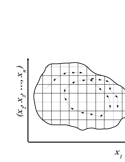
Figure 1: Pictorial representation of the phase space segmented into $n-$dimensional cells. Under the dynamics, the system’s trajectory moves from one cell to another.

The state space vector depends explicitly on time $t$ and the system moves from one point of the phase space to another with time. This motion of the system within the phase space can be used for the creation of the abstract network corresponding to the dynamics. Namely, we partition the phase space into $N$ segments $S_{j}$, $j=1,...N$. These segments are $n-$dimensional cells, as depicted in Fig. 1. For pictorial reasons the dimension corresponding to concentration $x_{1}$ is depicted on the $x-$ axis, while all other dimensions of the phase space $(d=2,\cdots n)$ are shown collapsed on the $y-$axis.

The partition of the phase space allows us to proceed to the definition of the abstract network characteristics. Namely, the phase space cells constitute the nodes of the network, with the dynamics governing the transitions from one node to another. An edge is drawn between two nodes $S_{i}$ and $S_{j}$ if the dynamics lead the system from cell $S_{i}$ to cell $S_{j}$ during one iteration step. The edge between $i$ and $j$ nodes is weighted with the frequency of jumps from cell $S_{i}$ to cell $S_{j}$ during the entire system integration time. The degree $D_{i}$ of the node (cell) $S_{i}$ is defined as the fraction of time that the system spends in space state cell $S_{i}$ and is equal to the sum of weights of all links starting from cell $S_{i}$. In the same spirit the abstract network transition matrix (or adjacency matrix or connectivity matrix) $M_{ij}$ is defined. The matrix element $M_{ij}$ denotes the fraction of transitions from cell $S_{i}$ to cell $S_{j}$ during the system integration. The degree $d_{j}$ of node $j$ can be written as a sum over the transition matrix elements,

$$d_{j}=\sum_{i=1}^{N}M_{ij},\>\>\>\{i,j\}=1,\cdots N.$$ (2)

In general $M_{ij}\neq M_{ji}$ and thus the abstract reactive networks belong to the class of directed networks. Loops (sometimes also called ”self-loops” or ”buckles”) may be present, since the dynamics might keep the system into the same cell after one integration step. In terms of the connectivity matrix elements, the presence of loops means $M_{ii}\neq 0$. In graph theory, graphs which contain loops are often called multigraphs.

In order to study the characteristics of a network quantitative indices are used, which can be computed from the transition matrix $M_{ij}$ . Based on these the network can be categorised in the general categories of random, small world or scaling network, etc. The most widely used properties are the clustering coefficients and the scaling exponents. The total number of nodes (cells) $N$ which cover the phase space is also called network size. The distribution of nodes which carry degree $d$ is denoted by $P(d)$ and describes the fractions of time the trajectory spends in the different parts of the phase space. The quantity $P(d)$ is called the degree distribution. It characterizes the network globally and classifies it to be scale-free if $P(d)$ has power law tails,

$$P(d)\sim d^{-\gamma}.$$ (3)

$\gamma$ is the power law exponent expressing the scale-free nature of the network and it is typically in the range $2<\gamma<3$, although in some cases $\gamma$ may lie outside this interval.

The local clustering coefficient $c_{l}$ describes the local network structure around the specific node $S_{l}$ and is defined as:

$$c_{l}=\frac{\sum_{i,j}M_{li}M_{ij}M_{jl}}{\sum_{i\not=j}M_{li}M_{jl}},\>\>\>\{i,j\}=1,\cdots N.$$ (4)

In Eq. (4) the numerator expresses the total weighted number of closed triangles originating from node $l$, while the denominator gives the maximum number of possible triangles originating on the same node grindrod:2002 ; saramaki:2007 .

The distribution of clustering coefficients $P(c)$ defines another critical exponent $\beta$, which takes a power law form in scale free networks,

$$P(c)\sim c^{-\beta}.$$ (5)

Watts and Strogatz have shown that $P(c)$ is exponentially decaying for random, uncorrelated networks watts:1998 ; ravasz:2003 .

The global clustering coefficient $c(N)$, defined as the average of the local clustering ones, characterises globally the connectivity in the network and in general depends on the size $N$ of the network,

$$c(N)=<c_{l}>=\frac{1}{N}\sum_{l=1}^{N}c_{l}.$$ (6)

$c(N)$ is important in the characterisation of typical networks. In particular, in random uncorrelated networks $c(N)$ decreases as watts:1998

$$c(N)\sim N^{-1}.$$ (7)

In the case of scale-free, highly clustered and complex networks Eq. (7) takes the general form

$$c(N)\sim N^{-\nu}.$$ (8)

It is worth here to understand how the phase space of the system behaves under different dynamical regimes and the form that the corresponding transition matrix takes. Indicative cases are:

1. When the phase state of the system contains a single attracting fixed point, then as $t\to\infty$ all initial states will converge to this attractor.

   $$\lim_{t\to\infty}\vec{X}(t) = \vec{X}_{fix}$$ (9)

   $$= (x_{1,f}(t),x_{2,f}(t),...x_{n,f}(t))$$

   In this case the transition matrix will only contain one single non-zero element, namely, the diagonal element which corresponds to the cell containing the attracting fixed point.

2. When the phase space of the system contains multiple attracting fixed points, then as $t\to\infty$ each initial state will converge to one of these attracting fixed points depending on the position of the state space vector at $t=0$. In this case the transition matrix will contain several scattered non-zero elements at the positions which correspond to the cells containing the attracting fixed points.

3. When the phase space of the system contains attracting periodic orbits (deterministic limit cycle) the state space vector will soon enter in one of those and will continue to move therein, following the orbit. Then only a subpart of the phase space is visited in the long run. The same is true for conservative systems where an infinite number of periodic orbits exist. These specific closed trajectories will be mirrored in the form of the transition matrix.

4. When the phase space of the system contains a chaotic attractor the state space vector eventually enters the attractor, is trapped therein and continues to move only in the area covered by the attractor. In this case also, the structure of the transition matrix and the critical exponents characterise the dynamics of the chaotic trajectory.

It must be noted here that in order to obtain numerically the correct transition matrix one should use very long integration times of the system so that the initial states will be forgotten and their overall contribution to the transition matrix will be negligible.

Although in the former two cases (1 and 2) the structure of the transition matrix is somewhat trivial, the same is not true in the latter two cases. Especially, the case of chaotic attractors should lead to nontrivial transition matrices and critical exponents, and its structure could be compatible with small world or scale free networks.

In the next section the particular reactive dynamics is specified as the Lattice Limit Cycle dynamics and its network characteristics are computed via KMC simulations which take into account spatial restrictions and stochastic effects.

III Working Example: The Lattice Limit Cycle Model

The LLC model has been previously studied and shown to possess many interesting properties: a) it has strong non-linearities of 4-th order, b) it is lattice compatible, in the sense that it can be directly applied on a lattice, without modifications on its dynamics, c) implies single-particle occupancy of a lattice site with the possibility of keeping certain sites empty d) both at the MF level and in the simulations it leads to dissipative oscillations e) gives rise to spatiotemporal pattern formations and fractal structures and f) gives rise to synchronization phenomena llc:2002 ; provata:2003 ; shabunin:2003 ; tsekouras:2006 . Due to its complex but tractable dynamics the LLC is an ideal candidate model for testing the abstract network approach and for studying the various reactive properties in view of the network characteristics.

In the next three subsections we recapitulate the most important features of the LLC model which will be used in the sequel for the study of the reactive abstract network properties.

III.1 The Model

The LLC model involves two types of interacting species (or particles) $X_{1},X_{2}$ and one virtual species $S$. The two interacting species participate in a series of reactions on an underlying surface, while the virtual species $S$ represents the empty surface sites. Without loss of generality, the surface is assumed to have the form of a square lattice of size $L\times L$, containing $L^{2}$ reactive sites. Each site can host at most one particle ( $X_{1}-state$ or $X_{2}-state$), or it can be empty ($S-state$). The reactive scheme is the following:

$$2X_{1}+2X_{2}\stackrel{{\scriptstyle p_{1}}}{{\rightarrow}}3X_{2}+S$$ (10a)

$$S+X_{1}\stackrel{{\scriptstyle p_{2}}}{{\rightarrow}}2X_{1}$$ (10b)

$$X_{2}+S\stackrel{{\scriptstyle p_{3}}}{{\rightarrow}}2S$$ (10c)

Each of the three reactions takes place with corresponding rate $p_{i}$; all rates will be translated into probabilities in the simulation process. The meaning of scheme (10c) is the following: when two particles of type $X_{1}$ are found within reaction distance with two particles of type $X_{2}$ they react with rate (probability) $p_{1}$ and one of the $X_{1}$ turns into $X_{2}$ while the other $X_{1}$ turns into $S$ (desorbs or dies). Likewise, when an empty site $S$ is found within reaction distance with a particle $X_{1}$ it reacts with probability $p_{2}$ and the empty site acquires an $X_{1}$ particle (adsorption). When an $X_{2}$ particle is found within reaction distance with an empty site $S$ it reacts desorbing with probability $p_{3}$. Reactive steps (10b) and (10c) are known in literature as cooperative birth and death processes, respectively.

The LLC scheme represents a non-equilibrium physicochemical process, with adsorption and desorption (or birth-and-death) mechanisms. The system is then considered as open and particles (species) can enter or leave the lattice. In some cases the particles can be immobile on the lattice and only reactions between particles are allowed within a certain distance. A common example is the disease spreading in (immobile) plants sokolov:2007 . In other cases some of the particles maybe mobile and diffuse on the lattice. A common example is the $CO$ oxidation on the surface of $Pt$. In this process $CO$ molecules and atomic oxygen $O$ are adsorbed on the surface site of $Pt$. The $CO$ molecules are highly mobile and diffuse on the lattice, while the $O$ atoms are strongly attached on the surface and they do not move pavlenko:2003 .

It is important to stress here that the realisation of step (10a) is difficult on lattice due to the requirement of simultaneous presence of the four specific particles, (two $X_{1}$ and two $X_{2}$) in the same local neighbourhood. And although at the MF level the dynamics of step (10a) is governed solely by the kinetic constant $p_{1}$, in the lattice realisation the local geometry and connectivity are shown to play an equally crucial role llc:2002 ; tsekouras:2006 . In particular, the dimensionality and type of lattice (square, triangular, cubic etc) is important in the sense that the critical points, the equilibrium states, the fixed points and the amplitude of oscillations depend quantitatively on the lattice type and dimensionality zhdanov:1999 ; provata:2005 ; zhdanov:1992 . However, the qualitative features are common in most lattice types, with the exception of the 1-D lattice, where the reaction scheme (10a) is difficult to be realised due to the restricted local geometry (only two first-neighbour sites for each node of the lattice). That is why, without loss of generality, we have decided to use the square lattice configuration as a substrate and to investigate the properties of the corresponding reactive abstract network.

III.2 Mean Field Equations

Deterministic MF is the traditional approach to reactive dynamics and although it does not describe the processes in detail it gives the general properties and tendencies of the phase space of the system. The MF equations describing the kinetic scheme (10c) are llc:2002 :

$$\frac{dx_{1}}{dt}=-2p_{1}x_{1}^{2}x_{2}^{2}+p_{2}sx_{1}$$ (11a)

$$\frac{dx_{2}}{dt}=p_{1}x_{1}^{2}x_{2}^{2}-p_{3}x_{2}s$$ (11b)

$$\frac{ds}{dt}=p_{1}x_{1}^{2}x_{2}^{2}-p_{2}x_{1}s+p_{3}sx_{2}$$ (11c)

where the small letters $x_{1},\>x_{2}$ and $s$ denote the temporal MF concentrations of the particles $X_{1},\>X_{2}$ and $S$, respectively. It is an inherent property of the system to satisfy the space conservation condition, i.e. that the total number of $X_{1}$, $X_{2}$ particles plus the empty sites $S$ should be conserved. This is also mirrored in the MF conservation condition $x_{1}+x_{2}+s=constant$ which is directly satisfied by the MF Eqs. (11). Customarily, the constant is identified as unity and then the variables $x_{1},\>x_{2},\>s$ are identified with the partial concentrations of the corresponding species. In a further simplification the system (11) is reduced to two equations, by eliminating the variable $s$ via the conservation condition $s=1-x_{1}-x_{2}$ llc:2002 . The reduced nonlinear system, also of 4-th order, reads:

$$\frac{dx_{1}}{dt} = -2p_{1}x_{1}^{2}x_{2}^{2}+p_{2}x_{1}(1-x_{1}-x_{2})$$

$$\frac{dx_{2}}{dt} = p_{1}x_{1}^{2}x_{2}^{2}-p_{3}x_{2}(1-x_{1}-x_{2})$$ (12)

Both original and reduced LLC have 4 fixed points $Q_{i}$, three of which are trivial. In the reduced representation the fixed points are:

$$Q_{1}=(0,0)$$ (13a)

$$Q_{2}=(0,1)$$ (13b)

$$Q_{3}=(1,0)$$ (13c)

$$Q_{4}=\left(\sqrt[3]{\frac{p_{3}^{2}}{p_{1}p_{2}}\left[1+K\right]}+\sqrt[3]{\frac{p_{3}^{2}}{p_{1}p_{2}}\left[1-K\right]},\right.$$

$$\left.\sqrt[3]{\frac{p_{2}^{2}}{8p_{1}p_{3}}\left[1+K\right]}+\sqrt[3]{\frac{p_{2}^{2}}{8p_{1}p_{3}}\left[1-K\right]}\right)$$ (13d)

with constant $K=\sqrt{1+(2p_{3}+p_{2})^{3}/(27p_{1}p_{2}p_{3})}$. While $Q_{i}$, $i=1,2,3$ are saddle fixed points, the stability of $Q_{4}$ is nontrivial. Depending on the parameter values, $Q_{4}$ undergoes a supercritical Hopf bifurcation giving rise to a limit cycle and periodic oscillations of the species concentrations.

The analysis so far refers solely to the deterministic MF description of the LLC, without taking into account spatial restrictions and stochastic effects, which will be briefly recapitulated in the next subsection.

III.3 Classical Kinetic Monte Carlo Simulations

As stated earlier in this study and in previous publications nicolis:1977 ; zhdanov:1999 ; llv:1999 the MF theory describes reactive systems only in the case of well mixed systems when every particle can interact equally with all other particles in the system, independently of their distance and position. Thus MF conditions are only achievable in well-stirred systems and they do not hold in systems where local effects need to be taken into account nicolis:1977 . For systems with spatial restrictions or with local stochastic effects the most detailed method is the probabilistic Master Equation approach, which accounts for all possible transitions of the system from one state to another, taking into account all spatial and stochastic effects. When the number of states is small, the probabilistic Master Equation is very efficient but it becomes intractable for large systems with many details in their spatial architecture. KMC methods are customarily designed to overcome this difficulty. They advance the system dynamics based on probabilistic transitions taking place by comparing the reaction rates with random numbers. The KMC method used here to describe the LLC model assumes single occupancy of every lattice site and interactions between nearest neighbouring sites. The rates are transformed into probabilities by dividing each one of them with the sum of the others. This transformation introduces a rescaling in time, without affecting the qualitative features of the system. Without loss of generality, the lattice here is assumed to be square with cyclic boundary conditions. The algorithm is described by the following steps:

1. A random site $(i,j)$ on the lattice is chosen.

2. If the site $(i,j)$ contains an $X_{1}$ particle and among its first neigbhours one $X_{1}$ particle and two $X_{2}$ particles are found, then the chosen $X_{1}$ particle and the neighbour $X_{1}$ particle are changed to $X_{2}$ and $S$, in random order. This step represents reaction scheme (10a) and takes place with probability $p_{1}$.

3. If the chosen site $(i,j)$ contains an $S$ particle (empty site) and a neighbouring site contains an $X_{1}$ particle, then the chosen site $(i,j)$ adsorbs an $X_{1}$ particle ($S$ is replaced by $X_{1}$) with probability $p_{2}$. This step is a cooperative adsorption or birth event and represents reaction scheme (10b).

4. If the chosen site $(i,j)$ contains an $X_{2}$ particle and a neighbouring site contains an $S$ particle (empty site), then the chosen $X_{2}$ desorbs ($S$ is replaced by $X_{2}$) with probability $p_{3}$. This step is a cooperative desorption or death event and represents reaction scheme (10c).

5. In all other cases the lattice remains unchanged.

6. An Elementary Time Step (ETS) is completed and the algorithm returns to step (1) for a new reaction ETS to start.

The time unit, Monte Carlo Step (MCS) of this process is defined as the number of ETS equal to the total number of lattice sites, i.e. for a square lattice of linear size $L$, $1\>\>MCS=L^{2}\>ETS$. With this definition each lattice site has the chance to react once, on average, in each MCS llc:2002 while at each ETS at most one reactive event takes place.

As shown in previous studies, while the MF dynamics dictates the presence of a limit cycle, after the system passes through a Hopf bifurcation, the reduction of the system on a low dimensional support together with the stochastic noise induced on the dynamics, lead to intermittent oscillations of the species concentrations on the lattice llc:2002 ; provata:2003 ; tsekouras:2006 . In Fig. 2 we present the temporal evolution of the LLC for the working parameter set $p_{1}=0.9585,p_{2}=0.016,p_{3}=0.026$, which lies beyond the Hopf bifurcation point. The black solid line denotes the MF dynamics: after an initial transitory time, the system generates regular cycles whose amplitude depends solely on the parameters $p_{i}$. The thick red line is generated by KMC simulations for the same parameter values and for system size $L\times L=2^{7}\times 2^{7}$. The periods (and frequencies) of the two time series are very close, but the KMC oscillations are irregular and show intermittent bursts. As previously discussed llc:2002 ; tsekouras:2006 the spatial extension of the system together with the limited range of the interactions divide the system into local oscillators which operate out of phase. Intermittent oscillations are observed for finite system sizes due to synchronisation of clusters of oscillators, while for large system sizes oscillations are suppressed due to cancellation of the random phases.

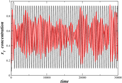
Figure 2: Temporal evolution of the $x_{1}$ concentration in LLC for parameter values $p_{1}=0.9585,p_{2}=0.016,p_{3}=0.026$ and lattice size $L=2^{7}$. The solid black line depicts the MF integration with purely periodic cycles, while the thick red line denotes the KMC simulations with irregular oscillations.

Having briefly recapitulated the detailed dynamics and spatiotemporal evolution of the LLC system we next examine the representation of this dynamics in terms of the corresponding abstract reactive network.

IV Network features of the Lattice Limit Cycle Model

For the realisation of the network it is possible to use an $n=1$ phase space representation, where only the $X_{1}$ (or only the $X_{2}$) species is considered or an $n=2$ representation where both species $X_{1}$ and $X_{2}$ are simultaneously recorded. We first give examples to show that many network features are the same whether we use the $n=1$ or the $n=2$ representation of the system.

Starting with the $n=1$ phase space, $X_{1}$ taken as an example, the phase space is partitioned into $N_{1}$ segments $S_{i}$, $i=1,\cdots N_{1}$ of size $\epsilon_{1}$, where

$$S_{i}=\left[x_{1}^{min}+i\epsilon_{1},x_{1}^{min}+(i+1)\epsilon_{1}\right]$$ (14)

These segments $S_{i}$ are identified as the $N_{1}$ discrete states of the system. In Eq. (14) $x_{1}^{min}$ is the minimum value of the variable $x_{1}$ and $x_{1}^{min}+N_{1}\epsilon_{1}=x_{1}^{max}$. Next, the transitions rates from segment (state) $S_{i}\to S_{j}$ are recorded during the KMC simulations in each Monte Carlo step. Based on these rates the transition matrix $M_{i,j}$ of size $N_{1}\times N_{1}$ can be written. This is the matrix that characterises the abstract network, its adjacency matrix. Since the domain of $x_{1}$ values is equipartinioned, some of the segments might not be visited, due to the dynamics, especially in the case where the $x_{1}-$domain is not fully connected. In this case some rows in the adjacency matrix will have all their elements equal to zero. Independently, the same construction can be designed for the variable $x_{2}$, whose phase space is segmented into $N_{2}$ nodes, while the corresponding adjacency matrix has size $N_{2}\times N_{2}$. Depending on the particular problem $N_{1}$ can be different from, or equal to $N_{2}$.

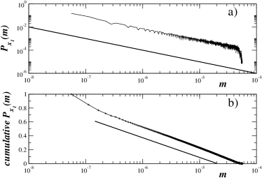
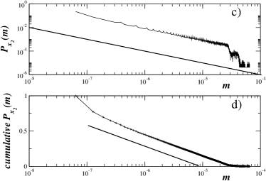
Figure 3: The size distribution of the elements of the transition matrix $M_{i,j}$ in the $n=1$ phase space representations: a) Size distribution of elements related to the variable $x_{1}$. The solid straight line indicates a power power law with exponent -1. b) Cumulative size distribution of elements related to the variable $x_{1}$. The solid line indicates a logarithmic dependence. c) Size distribution of elements related to the variable $x_{2}$. The solid straight line indicates a power power law with exponent -1. b) Cumulative size distribution of elements related to the variable $x_{2}$. The solid line indicates a logarithmic dependence. Parameter values are $p_{1}=0.9585,p_{2}=0.016,p_{3}=0.026$. The system size is $L\times L=2^{8}\times 2^{8}$ and $T=5\cdot 10^{7}$ Monte Carlo iteration steps were computed.

The size distribution of the $M_{i,j}$ elements (transition probabilities) is a very important statistical property of the network and can characterise its type. In Fig. 3a we plot the size distributions $P_{x_{1}}(m)$ which represents the probability that that a matrix element $M_{i,j}$ is in the interval $\left[m,m+dm\right]$ in the $n=1$ phase space representation. The parameter values are chosen as $p_{1}=0.9585,p_{2}=0.016,p_{3}=0.026$ and they are located in the region where intermittent oscillations are observed in the KMC simulations (see Fig. 2). In a double logarithmic scale the size distribution roughly follows a power law decay $P_{x_{1}}(m)\sim m^{-\gamma_{1}}$ with exponent $\gamma_{1}=1$. The value of the exponent $\gamma_{1}$ is further verified from the cumulative distribution shown in Fig. 3b. In a single logarithmic scale ($x-$axis) the cumulative distribution takes a linear form, indicating logarithmic dependence which further points to a power law exponent of the order of $\gamma_{1}=1$ for the original distribution. Similar behaviour is also recorded for the adjacency matrix corresponding to the $x_{2}$ variable. In Fig. 3c the $P_{x_{2}}(m)$ distribution is plotted in a double logarithmic scales. Similarly to Fig. 3a a scaling $\sim m^{-1}$ is followed, while in Fig. 3d the cumulative $P_{x_{2}}(m)$ distribution shows logarithmic dependence. This similar scaling is expected, since the two variables interact feeding each other and describe the dynamics of the same system.

The composite, $n=2$, network representation requires longer matrices since the phase space contains $N_{1}\times N_{2}$ nodes. Then the adjacency matrix has dimensions $N_{1}N_{2}\times N_{1}N_{2}$. In Fig. 4 the size distribution $P_{x_{1}x_{2}}$ of the $n=2$ adjacency matrix is plotted, for the KMC simulations using the working parameter set. The phase space is segmented in $64^{2}\times 64^{2}$ cells, using $N_{1}=N_{2}=64$. For comparison, the solid straight line in the double logarithmic scale represents a power law with exponent $\gamma_{1}=1.08$, which is consistent with the one observed in the $n=1$ representations. This nontrivial nonexponential decay of the size distribution of the transition matrix elements indicates that the abstract network which was constructed from the reactive process is a scale free network.

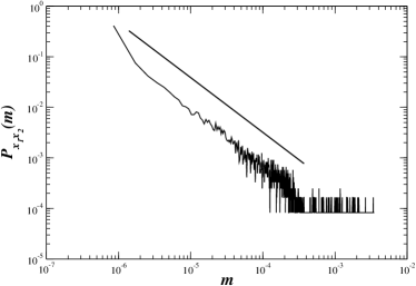
Figure 4: The size distribution of the elements of the composite transition matrix $M_{i,j}$ in the $n=2$ phase space representation. The straight solid line has slope -1.08. Parameter values and system size as in Fig. 3.

The degree distribution of the network nodes presents similar power law features. For the calculation of the degree distribution the $n=2$ representation is used, which accounts for the phase space properties in more detail. Because the degree $d_{j}$ of a specific node $j$ is composed as a sum over the transition matrix elements $M_{ij}$ (see Eq. (2)) and the size distribution of the matrix elements follows a power law then the degree distribution follows the same power law provided that the number of nodes $N$ is large enough. This is a direct consequence of the Generalised Central Limit Theorem which addresses distributions with power law tails. Indeed, in Fig. 5 the cumulative degree distribution of the network nodes is depicted and shows clear linear behaviour in semi-logarithmic scale. This is consistent with a power law degree distribution with exponent $\gamma=1$, as was also observed for the size distribution of the transition matrix elements. Note that if the matrix elements $M_{ij}$ are randomly and uniformly distributed then the degree distribution takes the shape of a noisy Gaussian (for finite size transition matrices).

Small degree distribution exponents, $\gamma<2$, are not unusual in real world phenomena; they have been observed and studied in particular in social networks (e-mail networks, package exchange networks etc.). It expresses the property of some networks where the total number of links or total weight carried by links grows faster than the number of nodes seyed:2006 .

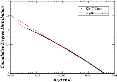
Figure 5: The degree distribution of the network nodes in the $n=2$ phase space representations. Parameter values and system size as in Fig. 3.

The distribution of clustering coefficients $P_{cc}$ also presents power law decay while the distribution $P_{cc}$ in the case of random and uniformly distributed transition matrix elements (links) $M_{ij}$ acquires a (noisy) Gaussian form. To further probe on the scale free properties of the abstract network we calculate the global (average) clustering coefficient as a function of the network size which is represented by the number of network nodes $N$. For simplicity we study the phase spaces of the $x_{1}$ and $x_{2}$ variables separately, to keep the size of the transition matrix to order of $N_{1(2)}\times N_{1(2)}$, for computational convenience. The phase spaces of the variables $x_{1}$ and $x_{2}$ are individually segmented in $N=32,\cdots 4096$ nodes and the corresponding average clustering coefficients $c_{1}(N)$ and $c_{2}(N)$ are computed. Figure 6 depicts the global clustering coefficient $c(N)=\left(c_{1}(N)+c_{2}(N)\right)/2$. In a double logarithmic scale $c(N)$ shows a power law decay with exponent $\nu\sim 1.46$. Similar values of the exponents are calculated for the individual clustering coefficients based on the $x_{1}$ and $x_{2}$ concentrations. Note that the exponent $\nu=1$ characterises random and uncorrelated networks watts:1998 , while the value $\nu=1.46$ computed here for the LLC model further verifies that this system is in the category of scale free networks.

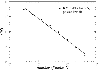
Figure 6: The average clustering coefficient as a function of the network size. Parameter values and system size as in Fig. 3.

The presence of power law exponents in the network representation of the reactive system KMC realisation on low dimensional lattice supports corroborates earlier investigations which demonstrate the formation of fractal patterns in the spatial arrangement of the reactants and products as a result of clustering of homologous particles and of cluster-cluster competition tsekouras:2006 ; sokolov:2007 . As stochastic interactions take place at the borderlines between different clusters these borderlines acquire complex fractal patterns and this spatial complexity, enhanced by the activity dynamics, shapes the form of the transition matrix. Thus the network power law exponents have their origin in the fractal spatial patterns developed as a result of the support restrictions on the dynamics of the reactive process.

V Conclusions

In the current study an abstract network construction is proposed for reactive systems based on the coarse graining of their phase space. The phase space of the reactive system, which is composed by the partial species concentrations, is divided into a numbers of segments which serve as the nodes of the abstract network. As described in sections II and IV, the trajectories which represent the temporal evolutions of the partial concentrations direct the system from one node to the next, determining the jump frequency between the different nodes and thus providing the adjacency matrix. Having the adjacency matrix it is then possible to compute all the network properties such as degree distribution, clustering coefficients, critical exponents and to classify the network as scale free, Erdos-Renyi, Small World etc.

As working example the Lattice Limit Cycle model is used which is an open, far from equilibrium, nonlinear, reactive system involving three reactive species participating in autocatalytic reactions, cooperative desorption and adsorption processes. The system is restricted on a two-dimensional lattice support with single particle lattice occupancy and local nearest neighbour interactions. The temporal evolution proceeds via KMC simulations which introduce stochastic factors in the system’s integration. Although the deterministic dynamics at the MF level predict dissipative oscillations of limit cycle type, the stochastic effects induced by the KMC dynamics lead to intermittent oscillations (with average amplitude depending on the system size) and the formation of spatiotemporal fractal patterns.

It is shown that the abstract phase space network corresponding to this reactive system is scale free and is characterised by a power law degree distribution $P(k)\sim k^{-\gamma}$ with exponent $\gamma\simeq 1$ while the average clustering coefficient $c(N)$ increases with the network size $N$ as $c(N)\sim N^{-\nu},\>\>\nu\simeq 1.46$. The origin of this nontrivial clustering is attributed to the cooperative nature of the reactions which form fractal spatiotemporal patterns on the lattice. The cooperative effect requires the presence of two different particles in adjacent lattice sites in order to react and this gives rise to segregation and to formation of clusters of homologous species. As interactions take place stochastically only in the borders between the clusters, surface roughening takes place producing fractal borderlines. These spontaneously produced fractals are at the origin of the scale free nature of the corresponding abstract phase space network.

The same general idea of abstract phase space networks can be applied to all reactive systems as well as in reaction-diffusion systems. The properties of the corresponding network reflect the spatial distribution of the reactants and together with the dynamics (nonlinearities) of the interactions determine the qualitative and quantitative properties of the network.

The construction of the abstract phase space network was based on the discrete time series which resulted by appropriately coarse graining the phase space of the concentrations variables ($x_{1}(t)$ or/and $x_{2}(t)$) and by following the dynamics as the system’s trajectory crosses from one cell to another in time. The discrete time series was the only information used for the subsequent construction of the abstract network. Equivalently, if a time series $f_{i},\>\>,i=1,...T$ is given, $f$ can be considered as the trajectory of an unknown dynamical system. Network analysis of time series has been the subject of various studies using different constructions of the phase space to study fractional Brownian motion and other processes lacasa:2009 ; yang:2007 ; dong:2013 . In the current LLC study the weighted network construction is based on the calculation of the total number of transitions between nodes and not on the local distances of the nodes on the reconstructed phase space. This way the adjacency matrix elements are calculated as the trajectory travels from node to node in the phase space, provided that the coarse grained time series of the concentrations $x_{i},\>>i=1,\cdots T$ is long enough to be considered as stationary (to have escaped the transient regime). This way any time series which has attained stationarity can be described by an abstract phase space network and the network characteristic exponents mirror the correlations of the time series. It would be interesting to investigate the network characteristics of time series originating from well known dynamical systems, including continuous chaotic flows and discrete maps and to analyse their dependence on the details of the phase space reconstruction.

VI Acknowledgments

The authors would like to thank Dr. G. Boulougouris, Prof. F. Diakonos and Prof. D. J. Frantzeskakis for useful discussions and critical comments. E. P. acknowledges a PhD fellowship from the NCSR “Demokritos”. This research has been co-financed by the European Union (European Social Fund – ESF) and Greek national funds through the Operational Program “Education and Lifelong Learning” of the National Strategic Reference Framework (NSRF) - Research Funding Program: THALES. Investing in knowledge society through the European Social Fund.

References

- (1) A. L. Barabasi, M. Newman and D. J. Watts, The Structure and Dynamics of Networks, Princeton University Press, Princeton, 2006.
- (2) A. Barrat, M. Barthelemy and A. Vespignani, Dynamical Processes on Complex Networks, Cambridge University Press, New York, 2008.
- (3) A. Barrat, M. Barthelemy, R. Pastor-Satorras and A. Vespignani, PNAS,101, 3747-3752 (2004).
- (4) I. Vragovic, E. Louis, A. Diaz-Guilera, Phys. Rev. E 71, 036122 (2005).
- (5) S. Yoon, S. Lee, S. H. Yook and Y. Kim, Phys. Rev. E 75,046114 (2007).
- (6) R. Albert, A. L. Barabasi, Rev. of Modern Physics, 74, 47-97 (2002).
- (7) S. N. Dorogovtsev, A. V. Goltsev, J. F. F. Mendes, Rev. of Modern Physics, 80, 1275-1335 (2008).
- (8) L. Lacasa, B. Luque, J. Luque and J. C. Nuno, Europhys. Lett., 86, 30001 (2009).
- (9) Y. Yang and H. Yang, Physica A, 387, 1381-1386 (2007).
- (10) Y. Dong, W. Huang, Z. Liu and S. Guan, Physica A, 392, 967-973 (2013).
- (11) A. Provata and C. Beck, Phys. Rev. E 86, 046101 (2012).
- (12) R. Sinatra, D. Condorelli and V. Latora, Phys. Rev. Letts., 105, 178702 (2010).
- (13) A. V. Shabunin, F. Baras, A. Provata, Physical Review E, 66, 036219 (2002).
- (14) A. Provata, G. A. Tsekouras, F. Diakonos, D. Frantzeskakis, F. Baras, A. V. Shabunin, V. Astakhov, Fluct. and Noise Letts., 3, L241-L250 (2003).
- (15) A. Shabunin, V. Astakhov, V. Demidov, A. Provata, F. Baras, G. Nicolis, V. Anishchenko, Chaos Solitons & Fractals, 15, 395-405 (2003).
- (16) I. Martinez-Forero, A. Pelaez-López and P. Villoslada PLoS ONE 5, e10823 (2010).
- (17) P. De Leenheer, D. Angeli anc E. D. Sontag, J. Math. Chem., 41, 295-314 (2007). DOI: 10.1007/s10910-006-9075-z
- (18) P.D. Kourdis, R. Steuer and D.A. Goussis, Physica, 239, 1789-1817, (2010).
- (19) A. Bernal and E. Daza, Current Computer-aided Drug Design, 7, 122-132 (2011).
- (20) P.V. Coveney, J. B. Swadling, J. A. D. Wattis and H. C. Greenwell, Chem. Soc. Rev., 41, 5430-5446 (2012).
- (21) P. Grindrod, Phys. Rev. E, 66, 066702 (2002).
- (22) J. Saramaki, M. Kivela, J. -P. Onnela, K. Kaski and J. Kertesz, Phys. Rev. E, 75, 027105 (2007).
- (23) D. J. Watts and S. H. Strogatz, Nature, 393 440-442 (1998).
- (24) E. Ravasz and A. -L. Barabasi, Phys. Rev. E, 67, 026112 (2003).
- (25) G. A. Tsekouras, A. Provata A, Europ. Phys. Jour. B, 52, 107-111 (2006).
- (26) E. B. Postnikov, I. M. Sokolov, Mathematical Biosciences, 208, 205 (2007).
- (27) N. Pavlenko, R. Imbihl, J. W. Evans, D. J. Liu, Phys. Rev. E,68, 016212 (2003).
- (28) V. P. Zhdanov, Physical Review E, 59, 6292 (1999).
- (29) A. Provata and V. K. Noussiou, Physical Review E, 72, 066108 (2005).
- (30) L. V. Lutsevich, O. A. Tkachenko and V. P. Zhdanov Langmuir, 8, 1757-1761 (1992).
- (31) G. Nicolis, I. Prigogine, Self-Organization in Nonequilibrium Systems, Wiley, New York, 1977.
- (32) A. Provata, G. Nicolis, F. Baras, J. Chem. Phys. 110, 8361 (1999).
- (33) H. Seyed-allaei, G. Bianconi and M. Marsili, Phys. Rev. E, 73, 046113 (2006).