Halo/Galaxy Bispectrum with Primordial non-Gaussianity from integrated Perturbation Theory (iPT)

Abstract

We derive a formula for the halo/galaxy bispectrum on the basis of the integrated Perturbation Theory (iPT). In addition to the gravity-induced non-Gaussianity, we consider the non-Gaussianity of the primordial curvature perturbations, and investigate in detail the effect of such primordial non-Gaussianity on the large-scale halo/galaxy bispectrum. In iPT, the effects of primordial non-Gaussianity are wholly encapsulated in the linear (primordial) polyspectra, and we systematically calculate the contributions to the large-scale behaviors arising from the three types of primordial bispectrum (local-, equilateral-, and orthogonal-types), and primordial trispectrum of the local-type non-Gaussianity. We find that the equilateral- and orthogonal-type non-Gaussianities show distinct scale-dependent behaviors which can dominate the gravity-induced non-Gaussianity at very large scales. For the local-type non-Gaussianity, higher-order loop corrections are found to give a significantly large contribution to the halo/galaxy bispectrum of the squeezed shape, and eventually dominate over the other contributions on large scales. A diagrammatic approach based on the iPT helps us to systematically investigate an impact of such higher-order contributions to the large-scale halo/galaxy bispectrum.

I Introduction

Hunting for the primordial non-Gaussianity in cosmological observations has been a focus of attention as a big impact on the cosmology. In March 2013, Planck collaboration has reported tight constraints on the non-linearity parameters which characterize the amplitude of the deviation from pure Gaussian statistics Ade:2013ydc . This result apparently implies that the cosmic microwave background (CMB) anisotropies measured by the Planck mission are very close to Gaussian, and may support the standard scenario of structure formation that the large-scale structure (LSS) of the Universe has emerged from tiny Gaussian fluctuations. Nevertheless, the constraints derived from LSS observations is still limited (e.g., Slosar:2008hx ; Giannantonio:2013uqa ), and at least as a cross check of the CMB results, it is worthwhile to further investigate the validity of this hypothesis precisely and independently from the LSS observations.

It is recently known that large-scale halo/galaxy distributions that trace the LSS provide a distinct information on the primordial non-Gaussianity. In particular, the scale dependence of halo/galaxy bias has been found to be a very powerful probe to search for a primordial non-Gaussianity (e.g., Dalal:2007cu ; Matarrese:2008nc ; Slosar:2008hx ; Giannantonio:2013uqa ). The most striking feature of the scale-dependent bias is that the effect appears even in the halo/galaxy power spectrum, and drastically change its shape and amplitude on large scales. This is in marked contrast to the case of CMB observations, where the fluctuations are still in the linear regime, and hence the bispectrum and other higher-order statistics of the CMB anisotropies are the direct probe of primordial non-Gaussianity.

In this paper, we are particularly interested in the halo/galaxy bispectrum. Notice that the influence of scale-dependent bias also appears in the halo/galaxy bispectrum and other polyspectra. Although the late-time gravitational evolution is known to induce the non-Gaussianity which inevitably dominates the primordial non-Gaussianity on small scales, a characteristic feature of the gravity-induced bispectrum basically differs from the one originating from the primordial non-Gaussianity. Further, due to the scale-dependent bias, the amplitude of halo/galaxy bispectrum may be enhanced, leading to a detectable signal on large scales (see, e.g., Ref. Jeong:2009vd ). In Ref. Sefusatti:2007ih ; Jeong:2009vd ; Sefusatti:2009qh , using the peak formalism and the local bias picture, the authors have derived the analytic expression for halo/galaxy bispectrum. On the other hand, the authors of Ref. Baldauf:2010vn make use of the peak-background split picture, and specifically studied the halo bispectrum in the presence of primordial local-type non-Gaussianity, characterized by the two constant parameters $f_{\rm NL}$ and $g_{\rm NL}$. Numerical study on the halo bispectrum has been also made with cosmological $N$-body simulation (see, e.g., Ref. Nishimichi:2009fs ). Still, however, most of works has restricted their attention to the local-type non-Gaussianity. With advent of high-precision LSS observations such as DES Abbott:2005bi , BigBOSS Schlegel:2011zz , LSST Abell:2009aa , EUCLID Laureijs:2011gra , and HSC/PFS (Sumire) Ellis:2012rn , it is important to give a systematic study on the prediction of bispectrum for various types of primordial non-Gaussianity.

In this paper, we systematically study the effect of the primordial non-Gaussianity on the bispectrum of the halos/galaxies, on the basis of the integrated Perturbation Theory (iPT) Matsubara:2011ck , which helps us to systematically derive a precise formula to connect the halo/galaxy clustering with the initial matter density field Matsubara:2012nc ; Yokoyama:2012az . With the iPT formalism, the non-local biasing effect can be incorporated into the statistical calculation of galaxies and halos in a straightforward manner. Further, in deriviing the effect of the primordial non-Gaussianity on the clustering of the halos, we do not need to introduce the peak-background split picture.

In Ref. Sato:2013qfa , the authors have compared an analytic formula for the correlation function of the halos based on the iPT formalism with numerical $N$-body simulation and found the agreement of those results with a high precision. Based on this formalism, we compute the halo bispectrum in the presence of local-, equilateral-, and orthogonal-type non-Gaussianities. Further, in case of the local-type non-Gaussianity, we include the effect of the primordial trispectrum characterized by two non-linearity parameters, $g_{\rm NL}$ and $\tau_{\rm NL}$. While we mainly present the results of iPT calculation at one-loop order (i.e., next-to-leading order), the two-loop order (i.e., next-to-next-leading order) contributions turns out to be important in several case. We will investigate in detail the impact of such higher-order contributions on the expected bispectrum signal on large scales.

This paper is organized as follows. In Sec. II, we begin by presenting a general formula for the bispectrum of the biased objects, which includes the effect of the primordial bispectrum and trispectrum up to the one-loop order in terms of iPT. Then, in Sec. III, we study in detail the formula for the halo bispectrum and separately consider the local-, equilateral and orthogonal-type non-Gaussianities. In section IV, we investigate the contributions of the higher order loops in terms of iPT. We discuss the comparison with the previous works where the bispectrum is obtained by other approaches and stress the utility of our systematic approach based on the iPT diagrammatic picture in section V. We also investigate the dependences of the redshift and the mass of halos. We devote the final section to summary. We plot the figures of this paper with adopting the best fit cosmological parameters taken from WMAP 9-year data Hinshaw:2012aka .

II Halo/galaxy Bispectrum from integrated Perturbation Theory

In this section, we give the formula for the bispectrum of galaxies and halos, based on the integrated perturbation theory (iPT). As we mentioned in the introduction, advantage of the integrated perturbation theory (iPT) is that the effect of non-local biasing can be incorporated into the statistical calculation of galaxies and halos in a straightforward manner. Ref. Sato:2013qfa has shown that an analytic formula for the correlation function of the halos based on the iPT agrees with $N$-body simulations in a good accuracy. Further, we do not need to introduce the peak-background split picture or peak formalism to derive the effect of the primordial non-Gaussianity in the clustering of the biased objects. Refs. Matsubara:2012nc ; Yokoyama:2012az have shown that the iPT formalism reproduces the previously known results for the scale-dependent bias as limiting cases of a general formula, and thus iPT gives a more general description for the scale-dependent bias.

In Sec. II.1, we first present the general expressions for the bispectrum at the one-loop order. We then derive the expressions of multi-point propagators in the large-scale limit in Sec. II.2, which will be the important building blocks to study the scale-dependent behavior of the bispectrum.

II.1 Bispectrum at one-loop order

We begin by defining the bispectrum of biased objects, $B_{X}$:

$$\langle\delta_{X}({\bf k}_{1})\delta_{X}({\bf k}_{2})\delta_{X}({\bf k}_{3})\rangle\equiv(2\pi)^{3}B_{X}({\bf k}_{1},{\bf k}_{2},{\bf k}_{3})\delta^{(3)}({\bf k}_{1}+{\bf k}_{2}+{\bf k}_{3})~{}.$$ (1)

The quantity $\delta_{X}$ is a Fourier transform of the number density field of the biased objects. In the iPT formalism, the multi-point propagators constitute the building blocks, and the perturbative expansion of the statistical quantities such as power spectrum and bispectrum are made with these propagators and the linear polyspectra. Denoting the $(n+1)$-point propagator of the biased objects by $\Gamma_{X}^{(n)}$, we define Matsubara:2011ck ; Bernardeau:2008fa

$$\Bigl{\langle}{\delta^{n}\delta_{X}({\bf k})\over\delta\delta_{\rm L}({\bf k}_{1})\delta\delta_{\rm L}({\bf k}_{2})\cdots\delta\delta_{\rm L}({\bf k}_{n})}\Bigr{\rangle}=(2\pi)^{3-3n}\delta({\bf k}_{1}+{\bf k}_{2}+\cdots+{\bf k}_{n})\Gamma_{X}^{(n)}({\bf k}_{1},{\bf k}_{2},\cdots,{\bf k}_{n}),$$ (2)

where $\delta_{\rm L}$ represents the (initial) linear density field. The multi-point propagator represents the influence on $\delta_{X}$ due to the infinitesimal variation for the initial density fields $\delta_{\rm L}$ through the non-linear mode coupling. It corresponds to the summation of all the loop contributions which are attached to each external vertex.

In order to discuss the effect of the primordial non-Gaussianity on the bispectrum of the biased objects, we here consider the perturbative expansion up to the one-loop order in iPT, which includes the contributions from the primordial trispectrum. Following the notation in the previous papers Matsubara:2011ck ; Matsubara:2012nc ; Yokoyama:2012az ; Matsubara:2013ofa , the bispectrum of the biased objects is expanded as

$$B_{X}({\bf k}_{1},{\bf k}_{2},{\bf k}_{3})=B_{\rm grav}^{\rm tree}+B_{\rm bis}^{\rm tree}+B_{\rm tris}+B_{\rm grav}^{{\rm loop},1}+B_{\rm grav}^{{\rm loop},2}+B_{\rm bis}^{{\rm loop},1}+B_{\rm bis}^{{\rm loop},2}+B_{\rm bis}^{{\rm loop},3}+\cdots,$$

with

$$B_{\rm grav}^{\rm tree} = \left[\Gamma_{X}^{(1)}({\bf k}_{1})\Gamma_{X}^{(1)}({\bf k}_{2})\Gamma_{X}^{(2)}(-{\bf k}_{1},-{\bf k}_{2})P_{\rm L}(k_{1})P_{\rm L}(k_{2})+2~{}{\rm perms.}\right],$$ (3)

$$B_{\rm bis}^{\rm tree} = \Gamma_{X}^{(1)}({\bf k}_{1})\Gamma_{X}^{(1)}({\bf k}_{2})\Gamma_{X}^{(1)}({\bf k}_{3})B_{\rm L}({\bf k}_{1},{\bf k}_{2},{\bf k}_{3}),$$ (5)

$$B_{\rm tris} = {1\over 2}\Gamma_{X}^{(1)}({\bf k}_{1})\Gamma_{X}^{(1)}({\bf k}_{2})\int{d^{3}p\over(2\pi)^{3}}\Gamma_{X}^{(2)}({\bf p},{\bf k}_{3}-{\bf p})T_{\rm L}({\bf k}_{1},{\bf k}_{2},{\bf p},{\bf k}_{3}-{\bf p})+2~{}{\rm perms.},$$ (7)

$$B_{\rm grav}^{{\rm loop},1} = \int{d^{3}p\over(2\pi)^{3}}\Gamma_{X}^{(2)}({\bf p},{\bf k}_{1}-{\bf p})\Gamma_{X}^{(2)}(-{\bf p},{\bf k}_{2}+{\bf p})\Gamma_{X}^{(2)}(-{\bf k}_{1}+{\bf p},-{\bf k}_{2}-{\bf p})P_{\rm L}(p)P_{\rm L}(|{\bf k}_{1}-{\bf p}|)P_{\rm L}(|{\bf k}_{2}+{\bf p}|),$$ (9)

$$B_{\rm grav}^{{\rm loop},2} = {1\over 2}\Gamma_{X}^{(1)}({\bf k}_{1})P_{\rm L}(k_{1})\int{d^{3}p\over(2\pi)^{3}}\Gamma_{X}^{(2)}({\bf p},{\bf k}_{2}-{\bf p})\Gamma_{X}^{(3)}(-{\bf k}_{1},-{\bf p},-{\bf k}_{2}+{\bf p})P_{\rm L}(p)P_{\rm L}(|{\bf k}_{2}-{\bf p}|)+5~{}{\rm perms.},$$ (11)

$$B_{\rm bis}^{{\rm loop},1} = {1\over 2}\Gamma_{X}^{(1)}({\bf k}_{1})\Gamma_{X}^{(1)}({\bf k}_{2})\int{d^{3}p\over(2\pi)^{3}}\Gamma_{X}^{(3)}(-{\bf k}_{1},{\bf p},-{\bf k}_{2}-{\bf p})P_{\rm L}(k_{1})B_{\rm L}({\bf k}_{2},{\bf p},-{\bf k}_{2}-{\bf p})+5~{}{\rm perms.},$$ (13)

$$B_{\rm bis}^{{\rm loop},2} = {1\over 2}\Gamma_{X}^{(1)}({\bf k}_{1})\Gamma_{X}^{(2)}(-{\bf k}_{1},-{\bf k}_{2})\int{d^{3}p\over(2\pi)^{3}}\Gamma_{X}^{(2)}({\bf p},{\bf k}_{2}-{\bf p})P_{\rm L}(k_{1})B_{\rm L}(-{\bf k}_{2},{\bf p},{\bf k}_{2}-{\bf p})+5~{}{\rm perms.},$$ (15)

$$B_{\rm bis}^{{\rm loop},3} = \Gamma_{X}^{(1)}({\bf k}_{1})\int{d^{3}p\over(2\pi)^{3}}\Gamma_{X}^{(2)}({\bf p},{\bf k}_{2}-{\bf p})\Gamma_{X}^{(2)}(-{\bf p},{\bf k}_{3}+{\bf p})P_{\rm L}(p)B_{\rm L}({\bf k}_{1},{\bf k}_{2}+{\bf p},{\bf k}_{3}-{\bf p})+2~{}{\rm perms.}.$$ (17)

The functions $P_{\rm L}$, $B_{\rm L}$ and $T_{\rm L}$ respectively denote the power-, bi- and tri-spectra of the linear density field, which are defined through

$$\langle\delta_{\rm L}({\bf k}_{1})\delta_{\rm L}({\bf k}_{2})\rangle = (2\pi)^{3}\delta({\bf k}_{1}+{\bf k}_{2})P_{\rm L}(k_{1}),$$ (18)

$$\langle\delta_{\rm L}({\bf k}_{1})\delta_{\rm L}({\bf k}_{2})\delta_{\rm L}({\bf k}_{3})\rangle = (2\pi)^{3}\delta({\bf k}_{1}+{\bf k}_{2}+{\bf k}_{3})B_{\rm L}(k_{1},k_{2},k_{3}),$$ (20)

$$\langle\delta_{\rm L}({\bf k}_{1})\delta_{\rm L}({\bf k}_{2})\delta_{\rm L}({\bf k}_{3})\delta_{\rm L}({\bf k}_{4})\rangle = (2\pi)^{3}\delta({\bf k}_{1}+{\bf k}_{2}+{\bf k}_{3}+{\bf k}_{4})T_{\rm L}(k_{1},k_{2},k_{3},k_{4}).$$ (22)

As we see in the above expression, in the iPT formalism, the bispectrum of the biased objects is expressed in terms of the primordial polyspectra as well as multi-point propagators. Hence, compared with the peak-background split picture, it is straightforward to take into account the effect of various types of the primordial non-Gaussianity whose statistical properties are encapsulated in the primordial polyspectra. Note that the linear density field is related to the primordial curvature perturbations $\Phi$ through the function ${\cal M}(k)$:

$$\delta_{\rm L}(k)={\cal M}(k)\Phi(k);\quad{\cal M}(k)={2\over 3}{D(z)\over D(z_{*})(1+z_{*})}{k^{2}T(k)\over H_{0}^{2}\Omega_{{\rm m}0}},$$ (23)

where $T(k)$, $D(z)$, $H_{0}$ and $\Omega_{{\rm m}0}$ are the transfer function, the linear growth factor, the Hubble parameter at present epoch, and the matter density parameter, respectively. Here $z_{*}$ denotes an arbitrary redshift at the matter-dominated era. With the relation (23), the linear power spectrum is given by

$$P_{\rm L}(k)=\left\{{\cal M}(k)\right\}^{2}P_{\Phi}(k),$$ (24)

with

$$\langle\Phi({\bf k})\Phi({\bf k}^{\prime})\rangle=(2\pi)^{3}\delta({\bf k}+{\bf k}^{\prime})P_{\Phi}(k).$$ (25)

In Fig. 1, diagrammatic representation of each term in Eq. (II.1) is shown. A double solid line connected with a grey circle, and a crossed circle glued to multiple single solid lines respectively indicate the multi-point propagator of biased objects $\Gamma^{(n)}_{X}$, and the correlator of the initial linear density field. As we have mentioned, with the multi-point propagator, all of the loop contributions which are attached to each external vertex are resummed, and the corresponding diagram does not have self-loops.

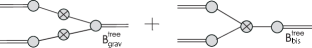
Figure 1: The diagrammatic representation for the bispectrum of the biased objects, $B_{X}$. The contributions up to the one-loop order in iPT are shown. A double solid line connected with a grey circle, and a crossed circle glued to multiple single solid lines represent the multi-point propagator of biased objects $\Gamma^{(n)}_{X}$, and the correlator of the initial linear density field, respectively.

II.2 Multi-point propagators in the large-scale limit

The multi-point propagator $\Gamma_{X}^{(n)}$ is defined as a fully non-perturbative quantity that contains all the important ingredients to describe the non-linear gravitational evolution and galaxy/halo bias properties. It is therefore difficult to evaluate it rigorously, however, for the large scales of our interest, perturbative treatment can work well, and we obtain the simplified expressions  Matsubara:2011ck ; Matsubara:2013ofa . In particular, taking the large-scale limit which means that the scale of interest ($\sim 1/k_{i}$) is much larger than the typical scale of the formation of the collapsed object ($\sim 1/p$ with $p$ being a variable of integration in Eq. (17)), we have

$$\Gamma_{X}^{(1)}({\bf k}) \approx 1+c_{1}^{\rm L}(k),$$ (26)

$$\Gamma_{X}^{(2)}({\bf k}_{1},{\bf k}_{2}) \approx F_{2}({\bf k}_{1},{\bf k}_{2})+\left(1+{{\bf k}_{1}\cdot{\bf k}_{2}\over k_{2}^{2}}\right)c_{1}^{\rm L}({\bf k}_{1})+\left(1+{{\bf k}_{1}\cdot{\bf k}_{2}\over k_{1}^{2}}\right)c_{1}^{\rm L}({\bf k}_{2})+c_{2}^{\rm L}({\bf k}_{1},{\bf k}_{2}),$$ (28)

$$\Gamma_{X}^{(3)}(-{\bf k}_{1},-{\bf p},-{\bf k}_{2}+{\bf p}) \approx -{{\bf k}_{1}\cdot{\bf k}_{3}\over k_{1}^{2}}c_{2}^{\rm L}(-{\bf p},{\bf p})+c_{3}^{\rm L}(-{\bf k}_{1},-{\bf p},-{\bf k}_{2}+{\bf p}),$$ (30)

where $F_{2}$ is the second-order kernel of standard perturbation theory, and we have ignored the contribution of $F_{3}$ to $\Gamma_{X}^{(3)}$. The expression of the kernel $F_{2}$ is given by

$$F_{2}({\bf k}_{1},{\bf k}_{2})={10\over 7}+\left({k_{2}\over k_{1}}+{k_{1}\over k_{2}}\right){{\bf k}_{1}\cdot{\bf k}_{2}\over k_{1}k_{2}}+{4\over 7}\left({{\bf k}_{1}\cdot{\bf k}_{2}\over k_{1}k_{2}}\right)^{2}.$$ (31)

Note that due to the symmetric property of $F_{2}$, we have

$$\Gamma_{X}^{(2)}(-{\bf p},{\bf p}) \approx c_{2}^{\rm L}(-{\bf p},{\bf p}).$$ (32)

In Eq. (30), the quantity $c_{n}^{\rm L}$ is a renormalized bias function defined in Lagrangian space, given by

$$c_{n}^{\rm L}({\bf k}_{1},{\bf k}_{2},\cdots,{\bf k}_{n})=(2\pi)^{3n}\int{d^{3}k^{\prime}\over(2\pi)^{3}}\Biggl{\langle}{\delta^{n}\delta_{X}^{\rm L}({\bf k}^{\prime})\over\delta\delta_{\rm L}({\bf k}_{1})\delta\delta_{\rm L}({\bf k}_{2})\cdots\delta\delta_{\rm L}({\bf k}_{n})}\Biggr{\rangle},$$ (33)

with $\delta_{X}^{\rm L}$ being the number density field of biased objects defined in Lagrangian space.

So far, the derivation of the formulae above is quite general, and Eq. (17), together with the large-scale limit of multipoint propagators (30) with renormalized bias function (33), can be applied to any biased objects in order to study the scale-dependence of the bispectrum. For a quantitative investigation of the large-scale behaviors of the bispectrum, in what follows, we specifically consider the halo clustering, whose statistical properties are well-studied analytically and numerically. In the case of halos, the analytic expressions for the renormalized bias function $c_{n}^{\rm L}$ has been already derived Matsubara:2011ck ; Matsubara:2013ofa , and we can quantitatively predict the amplitude of the halo bispectrum, which will be compared with $N$-body simulations. Since the galaxies mainly form inside the halos, for our interest of the large-scale limit, we expect that qualitatively similar features found in the case of halo bispectrum hold in the case of galaxy bispectrum.

Adopting a simple model of non-local halo bias proposed by Ref. Matsubara:2011ck ; Matsubara:2013ofa , the renormalized bias function for halos with mass $M$ is given by

$$c_{n}^{\rm L}({\bf k}_{1},\cdots,{\bf k}_{n})={A_{n}(M)\over\delta_{c}^{n}}W(k_{1};M)\cdots W(k_{n};M)+{A_{n-1}(M)\sigma_{M}^{n}\over\delta_{c}^{n}}{d\over d\ln\sigma_{M}}\left[{W(k_{1};M)\cdots W(k_{n};M)\over\sigma_{M}^{n}}\right],$$ (34)

where $\delta_{c}(\simeq 1.686)$ is the so-called critical density of the spherical collapse model, $W(k;M)$ is the window function smoothed with the mass scale $M=4\pi\rho R^{3}/3$, and $\sigma_{M}$ is the variance of density fluctuations on the mass scale $M$. Here, a function $A_{n}(M)$ is defined by

$$A_{n}(M)\equiv\sum^{n}_{j=0}{n!\over j!}\delta_{c}^{j}b_{j}^{\rm L}(M),$$ (35)

with $b_{j}^{\rm L}(M)$ being the $n$-th order scale-independent Lagrangian bias parameter which is constructed from the universal mass function as

$$b_{j}^{\rm L}(M)=\left(-\sigma_{M}\right)^{-n}f_{\rm MF}^{-1}{d^{n}\over d\nu^{n}}\left(f_{\rm MF}(\nu)\right).$$ (36)

Throughout the paper, we adopt the fitting formula by Sheth and Tormen Sheth:1999mn for the halo mass function $f_{\rm MF}$, and explicitly compute the halo bispectrum:

$$f_{\rm MF}(\nu)=f_{\rm ST}(\nu)=A(p)\sqrt{{2\over\pi}}\left[1+(q\nu^{2})^{-p}\right]\sqrt{q}\nu e^{-q\nu^{2}/2},$$ (37)

where $\nu=\delta_{c}/\sigma_{M}$, $p=0.3$, $q=0.707$ and the normalization factor $A(p)=\left[1+\Gamma(1/2-p)/(\sqrt{\pi}2^{p})\right]^{-1}$. In Appendix A, we discuss the influence of the different choice of the mass functions on the final result of halo bispectrum. Note finally that in the large scale limit where $k_{1},k_{2},k_{3}\to 0$, the window function and its derivative asymptotically approach $W(k_{i};R)\to 1$ and $dW(k_{i};R)/d\ln\sigma_{M}\to 0$, and hence the renormalized bias function does not have significant scale-dependence.

III Results for each type of primordial non-Gaussianity

Let us now study in detail the formula for bispectrum of the biased objects given by Eq. (17), especially focusing on the case of halos. In what follows, we separately consider the three types of primordial non-Gaussianity; local-, equilateral-, and orthogonal-type characterized by the specific shape of the bispectrum $B_{\rm L}$ and/or trispectrum $T_{\rm L}$.

III.1 Local-type non-Gaussianity

In the primordial local-type non-Gaussianity, the bispectrum and trispectrum of linear matter density field are respectively characterized by

$$B_{\rm L}(k_{1},k_{2},k_{3}) = {\cal M}(k_{1}){\cal M}(k_{2}){\cal M}(k_{3})2f_{\rm NL}\left[P_{\Phi}(k_{1})P_{\Phi}(k_{2})+P_{\Phi}(k_{2})P_{\Phi}(k_{3})+P_{\Phi}(k_{3})P_{\Phi}(k_{1})\right],$$ (38)

and

$$T_{\rm L}(k_{1},k_{2},k_{3},k_{4}) = {\cal M}(k_{1}){\cal M}(k_{2}){\cal M}(k_{3}){\cal M}(k_{4})\Bigl{\{}6g_{\rm NL}\left[P_{\Phi}(k_{1})P_{\Phi}(k_{2})P_{\Phi}(k_{3})+3~{}{\rm perms.}\right]$$ (41)

$$\qquad\qquad\qquad\qquad\qquad\qquad\qquad+{25\over 9}\tau_{\rm NL}\left[P_{\Phi}(k_{1})P_{\Phi}(k_{2})P_{\Phi}(k_{13})+11~{}{\rm perms.}\right]\Bigr{\}},$$

with $k_{ij}=|{\bf k}_{i}+{\bf k}_{j}|$. Here, the constant parameters, $f_{\rm NL}$, $g_{\rm NL}$ and $\tau_{\rm NL}$, are called non-linearity parameters. If one considers the case with single-sourced primordial curvature perturbations characterized by $\Phi=\Phi_{G}+f_{\rm NL}(\Phi_{G}^{2}-\langle\Phi_{G}^{2}\rangle)+g_{\rm NL}\Phi_{G}^{3}$, the non-linearity parameter $\tau_{\rm NL}$ is related to the leading-order one $f_{\rm NL}$ through $\tau_{\rm NL}=36f_{\rm NL}^{2}/25$, which is nothing but the consistency relation. Note that this relation does not hold in general. In cases with multi-sourced curvature perturbations, we obtain the inequality, $\tau_{\rm NL}\geq 36f_{\rm NL}^{2}/25$ Suyama:2007bg ; Suyama:2010uj ; Sugiyama:2011jt ; Bramante:2011zr ; Sugiyama:2012tr . The consistency relation or inequality can be checked with the measurement of both the power spectrum of biased object and cross spectrum between the biased object and the matter density field Yokoyama:2012az (see also Refs.Gong:2011gx ; Nishimichi:2012da ; Baumann:2012bc ; Tseliakhovich:2010kf ; Biagetti:2012xy ; Smith:2010gx ). Below, in evaluating the halo bispectrum, we simply assume that the consistency relation holds, $\tau_{\rm NL}=36f_{\rm NL}^{2}/25$, and present the results.

Substituting the expressions of $P_{\rm L}$, $B_{\rm L}$ and $T_{\rm L}$ into Eq. (17), each term of the bispectrum of the biased objects for the primordial local-type non-Gaussianity is evaluated as follows. Apart from the first term in Eq. (17), the contribution $B_{\rm bis}^{\rm tree}$ becomes

$$B_{\rm bis}^{\rm tree} = 2f_{\rm NL}\Gamma_{X}^{(1)}({\bf k}_{1})\Gamma_{X}^{(1)}({\bf k}_{2})\Gamma_{X}^{(1)}({\bf k}_{3}){\cal M}(k_{1}){\cal M}(k_{2}){\cal M}(k_{3})\biggl{[}P_{\Phi}(k_{1})P_{\Phi}(k_{2})+2~{}{\rm perms.}\biggr{]}.$$ (42)

The third term in Eq. (17), $B_{\rm tris}$, is separately evaluated as:

$$B_{\rm tris} \equiv B_{g_{\rm NL}}+B_{\tau_{\rm NL}},$$

with

$$B_{g_{\rm NL}} = 6g_{\rm NL}\Biggl{\{}\Gamma_{X}^{(1)}({\bf k}_{1})\Gamma_{X}^{(1)}({\bf k}_{2}){\cal M}(k_{1}){\cal M}(k_{2})P_{\Phi}(k_{1})P_{\Phi}(k_{2})$$ (45)

$$\times\int{d^{3}p\over(2\pi)^{3}}\Gamma_{X}^{(2)}({\bf p},{\bf k}_{3}-{\bf p}){\cal M}(p){\cal M}(|{\bf k}_{3}-{\bf p}|)P_{\Phi}(p)\left[1+{1\over 2}\left({P_{\Phi}(|{\bf k}_{3}-{\bf p}|)\over P_{\Phi}(k_{1})}+{P_{\Phi}(|{\bf k}_{3}-{\bf p}|)\over P_{\Phi}(k_{2})}\right)\right]+2~{}{\rm perms.}\Biggr{\}},$$

$$B_{\tau_{\rm NL}} = {25\over 9}\tau_{\rm NL}\Biggl{\{}\Gamma_{X}^{(1)}({\bf k}_{1})\Gamma_{X}^{(1)}({\bf k}_{2}){\cal M}(k_{1}){\cal M}(k_{2})\left[P_{\Phi}(k_{1})+P_{\Phi}(k_{2})\right]P_{\Phi}(k_{3})$$ (57)

$$\qquad\qquad\qquad\times\int{d^{3}p\over(2\pi)^{3}}\Gamma_{X}^{(2)}({\bf p},{\bf k}_{3}-{\bf p}){\cal M}(p){\cal M}(|{\bf k}_{3}-{\bf p}|)P_{\Phi}(p)+2~{}{\rm perms.}\Biggr{\}}$$

$$+{25\over 9}\tau_{\rm NL}\Biggl{\{}\Gamma_{X}^{(1)}({\bf k}_{1})\Gamma_{X}^{(1)}({\bf k}_{2}){\cal M}(k_{1}){\cal M}(k_{2})P_{\Phi}(k_{1})P_{\Phi}(k_{2})$$

$$\qquad\qquad\qquad\times\int{d^{3}p\over(2\pi)^{3}}\Gamma_{X}^{(2)}({\bf p},{\bf k}_{3}-{\bf p}){\cal M}(p){\cal M}(|{\bf k}_{3}-{\bf p}|)P_{\Phi}(|{\bf k}_{1}+{\bf p}|)+2~{}{\rm perms.}\Biggr{\}}$$

$$+{25\over 9}\tau_{\rm NL}\Biggl{\{}\Biggl{[}\Gamma_{X}^{(1)}({\bf k}_{1})\Gamma_{X}^{(1)}({\bf k}_{2}){\cal M}(k_{1}){\cal M}(k_{2})P_{\Phi}(k_{1})\int{d^{3}p\over(2\pi)^{3}}\Gamma_{X}^{(2)}({\bf p},{\bf k}_{3}-{\bf p})$$

$$\qquad\times{\cal M}(p){\cal M}(|{\bf k}_{3}-{\bf p}|)P_{\Phi}(p)P_{\Phi}(|{\bf k}_{3}-{\bf p}|)\left[1+{P_{\Phi}(|{\bf k}_{2}+{\bf p}|)\over 2P_{\Phi}(k_{1})}\right]+({\bf k}_{1}\leftrightarrow{\bf k}_{2})\Biggr{]}+2~{}{\rm perms.}\Biggr{\}}.$$

The remaining one-loop contributions that are linearly proportional to $f_{\rm NL}$ are $B_{\rm bis}^{{\rm loop},1}$, $B_{\rm bis}^{{\rm loop},2}$, and $B_{\rm bis}^{{\rm loop},3}$, which can be respectively recast as

$$B_{\rm bis}^{{\rm loop},1} = 2f_{\rm NL}\Biggl{\{}\Gamma_{X}^{(1)}({\bf k}_{1})\Gamma_{X}^{(1)}({\bf k}_{2})\Biggl{[}P_{\rm L}(k_{1}){P_{\rm L}(k_{2})\over{\cal M}(k_{2})}\int{d^{3}p\over(2\pi)^{3}}\Gamma_{X}^{(3)}(-{\bf k}_{1},-{\bf p},-{\bf k}_{2}+{\bf p})$$ (60)

$$\qquad\qquad\qquad\times{\cal M}(p){\cal M}(|{\bf k}_{2}-{\bf p}|)P_{\Phi}(p)\left(1+{P_{\Phi}(|{\bf k}_{2}-{\bf p}|)\over 2P_{\Phi}(k_{2})}\right)+({\bf k}_{1}\leftrightarrow{\bf k}_{2})\Biggr{]}+2~{}{\rm perms.}\Biggr{\}},$$

$$B_{\rm bis}^{{\rm loop},2} = 2f_{\rm NL}\Biggl{\{}\Gamma_{X}^{(1)}({\bf k}_{1})\Biggl{[}\Gamma_{X}^{(2)}({\bf k}_{1},{\bf k}_{2})P_{\rm L}(k_{1}){P_{\rm L}(k_{2})\over{\cal M}(k_{2})}$$ (64)

$$\times\int{d^{3}p\over(2\pi)^{3}}\Gamma_{X}^{(2)}({\bf p},{\bf k}_{2}-{\bf p}){\cal M}(p){\cal M}(|{\bf k}_{2}-{\bf p}|)P_{\Phi}(p)\left(1+{P_{\Phi}(|{\bf k}_{2}-{\bf p}|)\over 2P_{\Phi}(k_{2})}\right)+({\bf k}_{2}\leftrightarrow{\bf k}_{3})\Biggr{]}+2~{}{\rm perms.}\Biggr{\}},$$

$$B_{\rm bis}^{{\rm loop},3} = f_{\rm NL}\Biggl{\{}\Gamma_{X}^{(1)}({\bf k}_{1}){\cal M}(k_{1})P_{\Phi}(k_{1})\Biggl{[}\int{d^{3}p\over(2\pi)^{3}}\Gamma_{X}^{(2)}({\bf p},{\bf k}_{2}-{\bf p})\Gamma_{X}^{(2)}(-{\bf p},{\bf k}_{3}+{\bf p})P_{\rm L}(p){\cal M}(|{\bf k}_{2}-{\bf p}|){\cal M}(|{\bf k}_{3}+{\bf p}|)$$ (68)

$$\qquad\times\left(P_{\Phi}(|{\bf k}_{2}-{\bf p}|)+P_{\Phi}(|{\bf k}_{3}+{\bf p}|)+{P_{\Phi}(|{\bf k}_{3}+{\bf p}|)P_{\Phi}(|{\bf k}_{2}-{\bf p}|)\over P_{\Phi}(k_{1})}\right)+({\bf k}_{2}\leftrightarrow{\bf k}_{3})\Biggr{]}+2~{}{\rm perms.}\Biggr{\}}.$$

On small scales, the halo/galaxy bispectrum is generically dominated by the non-linearity of gravitational evolution, and the contribution coming from the higher-order loops becomes non-negligible. In this respect, similar to the power spectrum case, large-scales are the only window where the effect of the primordial non-Gaussianity would be significant, giving rise to a detectable signature on the bispectrum. Let us then consider the large-scale limit in which all of the wave numbers $k_{1}$, $k_{2}$, and $k_{3}$ are much smaller than the typical scale of the biased object (halo). In this limit, we obtain the approximate expressions for $B_{g_{\rm NL}}$ and $B_{\tau_{\rm NL}}$:

$$B_{g_{\rm NL}} \approx 6g_{\rm NL}\left[\Gamma_{X}^{(1)}({\bf k}_{1})\Gamma_{X}^{(1)}({\bf k}_{2}){\cal M}(k_{1}){\cal M}(k_{2})P_{\Phi}(k_{1})P_{\Phi}(k_{2})\int{d^{3}p\over(2\pi)^{3}}\Gamma_{X}^{(2)}({\bf p},-{\bf p})P_{\rm L}(p)+2~{}{\rm perms.}\right],$$ (69)

$$B_{\tau_{\rm NL}} \approx {25\over 9}\tau_{\rm NL}\Bigl{\{}\Gamma_{X}^{(1)}({\bf k}_{1})\Gamma_{X}^{(1)}({\bf k}_{2}){\cal M}(k_{1}){\cal M}(k_{2})$$ (75)

$$\qquad\times\left[P_{\Phi}(k_{1})P_{\Phi}(k_{2})+P_{\Phi}(k_{2})P_{\Phi}(k_{3})+P_{\Phi}(k_{3})P_{\Phi}(k_{1})\right]\int{d^{3}p\over(2\pi)^{3}}\Gamma_{X}^{(2)}({\bf p},-{\bf p})P_{\rm L}(p)+2~{}{\rm perms.}\Bigr{\}}$$

$$+{25\over 9}\tau_{\rm NL}\Bigl{\{}\Gamma_{X}^{(1)}({\bf k}_{1})\Gamma_{X}^{(1)}({\bf k}_{2}){\cal M}(k_{1}){\cal M}(k_{2})\left[P_{\Phi}(k_{1})+P_{\Phi}(k_{2})\right]\int{d^{3}p\over(2\pi)^{3}}\Gamma_{X}^{(2)}({\bf p},-{\bf p})P_{\rm L}(p)P_{\Phi}(p)+2~{}{\rm perms.}\Bigr{\}}.$$

Also, the rest of the one-loop contributions is approximately described as

$$B_{\rm grav}^{{\rm loop},1} \approx \int{d^{3}p\over(2\pi)^{3}}\left[\Gamma_{X}^{(2)}({\bf p},-{\bf p})P_{\rm L}(p)\right]^{3},$$ (76)

$$B_{\rm grav}^{{\rm loop},2} \approx {1\over 2}\left[\Gamma_{X}^{(1)}({\bf k}_{1})P_{\rm L}(k_{1})\int{d^{3}p\over(2\pi)^{3}}\Gamma_{X}^{(2)}({\bf p},-{\bf p})\Gamma_{X}^{(3)}(-{\bf k}_{1},-{\bf p},-{\bf k}_{2}+{\bf p})P_{\rm L}(p)^{2}+~{}5~{}{\rm perms.}\right],$$ (78)

$$B_{\rm bis}^{{\rm loop},1} \approx 2f_{\rm NL}\left[\Gamma_{X}^{(1)}({\bf k}_{1})\Gamma_{X}^{(1)}({\bf k}_{2})P_{\rm L}(k_{1}){P_{\rm L}(k_{2})\over{\cal M}(k_{2})}\int{d^{3}p\over(2\pi)^{3}}\Gamma_{X}^{(3)}(-{\bf k}_{1},-{\bf p},-{\bf k}_{2}+{\bf p})P_{\rm L}(p)+5~{}{\rm perms.}\right],$$ (80)

$$B_{\rm bis}^{{\rm loop},2} \approx 2f_{\rm NL}\left[\Gamma_{X}^{(1)}({\bf k}_{1})\Gamma_{X}^{(2)}({\bf k}_{1},{\bf k}_{2})P_{\rm L}(k_{1}){P_{\rm L}(k_{2})\over{\cal M}(k_{2})}\int{d^{3}p\over(2\pi)^{3}}\Gamma_{X}^{(2)}({\bf p},-{\bf p})P_{\rm L}(p)+5~{}{\rm perms.}\right],$$ (82)

$$B_{\rm bis}^{{\rm loop},3} \approx 4f_{\rm NL}\left\{\Gamma_{X}^{(1)}({\bf k}_{1}){P_{\rm L}(k_{1})\over{\cal M}(k_{1})}\int{d^{3}p\over(2\pi)^{3}}\left[\Gamma_{X}^{(2)}({\bf p},-{\bf p})P_{\rm L}(p)\right]^{2}+2~{}{\rm perms.}\right\},$$ (84)

where we have used the fact that $P_{\Phi}(p)/P_{\Phi}(k_{i})\sim k_{i}^{3}/p^{3}\to 0$.

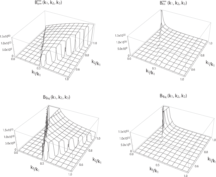
Figure 2: The shapes of $B_{\rm grav}^{\rm tree}$, $B_{\rm bis}^{\rm tree}$, $B_{g_{\rm NL}}$ and $B_{\tau_{\rm NL}}$ as functions of $k_{3}/k_{1}$ and $k_{2}/k_{1}$ in momentum space for $k_{1}=0.005\,h$ Mpc^-1.

As examples of the shape of each contribution in $k$-space, in Fig. 2, we plot $B_{\rm grav}^{\rm tree}$, $B_{\rm bis}^{\rm tree}$, $B_{g_{\rm NL}}$ and $B_{\tau_{\rm NL}}$ for fixed $k_{1}=0.005\,h$ Mpc^-1 . Here, the redshift and the mass scale of halos are set to $z=1.0$ and $M=5\times 10^{13}h^{-1}M_{\odot}$, respectively, and we assume $k_{1}\geq k_{2}\geq k_{3}$ and $k_{3}\geq k_{1}-k_{2}$ because of the triangle condition. In the following discussion, we fix the redshift and the mass scale of halos to be above values. In Discussion V.1, we investigate the redshift and the mass dependences of the halo bispectrum. As shown in this figure, we find that the contributions of the primordial non-Gaussianity become dominant and have large amplitudes in the squeezed limit, while the leading-order effect of gravitational non-linearity appears in an equilateral shape. To clarify the scale-dependence of their contributions, let us introduce the isosceles configuration given by $k\equiv k_{1}=k_{2}=\alpha k_{3}$. A large $\alpha$ corresponds to the squeezed shape. Then, for small $k$ and large $\alpha$, the dominant scale-dependence of each contribution is simply given in terms of $k$ and $\alpha$ as

$$B_{\rm grav}^{\rm tree}\propto k^{2}\alpha^{0},~{}B_{\rm bis}^{\rm tree}\propto k^{0}\alpha^{1},~{}B_{g_{\rm NL}}\propto k^{-2}\alpha^{1},~{}B_{\tau_{\rm NL}} \propto k^{-2}\alpha^{3}.$$ (85)

and

$$B_{\rm grav}^{{\rm loop},1}\propto k^{0}\alpha^{0},~{}B_{\rm grav}^{{\rm loop},2}\propto k^{1}\alpha^{0},~{}B_{\rm bis}^{{\rm loop},1}\propto k^{0}\alpha^{1},~{}B_{\rm bis}^{{\rm loop},2}\propto k^{0}\alpha^{1},~{}B_{\rm bis}^{{\rm loop},3}\propto k^{-1}\alpha^{1},$$ (86)

where we have assumed that the power spectrum of the primordial fluctuations is scale-invariant, that is, $P_{\Phi}(k)\propto k^{-3}$. From the above equations, we find that the contributions from the non-linearity of the gravitational evolution have positive powers of $k$ and they decrease as $k$ decreases. We also see that the contributions from the primordial bispectrum have similar $k$ and $\alpha$-dependences except for $B_{\rm bis}^{{\rm loop},3}$. As we will see later, $B_{\rm bis}^{{\rm loop},3}$ is suppressed on large scales compared with other $B_{\rm bis}$ contributions, and the total contribution from the primordial bispectrum can be simply scaled as $\propto k^{0}\alpha^{1}$. Such scale-dependent behaviors on large scales have been discussed in previous works Sefusatti:2007ih ; Jeong:2009vd ; Sefusatti:2009qh ; Nishimichi:2009fs ; Baldauf:2010vn , and our result is consistent with their results. On the other hand, the contributions from the primordial trispectrum characterized by $g_{\rm NL}$ and $\tau_{\rm NL}$ (i.e., $B_{g_{\rm NL}}$ and $B_{\tau_{\rm NL}}$) have the $k^{-2}$-dependence, and hence we expect that on large scales they become dominant in the halo bispectrum. Moreover, compared with contributions from primordial bispectrum (i.e., $B_{\rm bis}^{\rm tree}$, $B_{\rm bis}^{{\rm loop},1}$, $B_{\rm bis}^{{\rm loop},2}$, and $B_{\rm bis}^{{\rm loop},3}$) and the term $B_{g_{\rm NL}}$, the term $B_{\tau_{\rm NL}}$ has a larger power of $\alpha$, and hence in the squeezed limit ($\alpha\gg 1$), this can dominate the halo bispectrum on large scales.

In left panel of Fig. 3, we plot the contributions $B_{\rm grav}^{\rm tree}$ (black thin dashed line), $B_{\rm bis}^{\rm tree}$ (red thick line), $B_{g_{\rm NL}}$ (blue thick dashed line), and $B_{\tau_{\rm NL}}$ (green thick dotted line), as functions of the wavenumber $k$ with $\alpha=10$. The non-linearity parameters are given by $f_{\rm NL}=10$, $g_{\rm NL}=10^{4}$ and $\tau_{\rm NL}=36f_{\rm NL}^{2}/25$. The asymptotic $k$-dependence expressed in Eq. (85) is found to be realized at $k\lesssim 0.02\,h$ Mpc^-1. With the currently allowed values of the non-linearity parameters, the contributions of the primordial non-Gaussianitiy can dominate the halo bispectrum at $k\lesssim 0.01\,h$ Mpc^-1. On the other hand, At $k\gtrsim 0.02\,h$ Mpc^-1, the scale-dependence of each contribution gradually changes and deviates from the one in Eq. (85). This is simply due to the behavior of the transfer function $T(k)$, and thus the approximation based on the large-scale limit would become invalid at $k\sim 0.1\,h$ Mpc^-1.

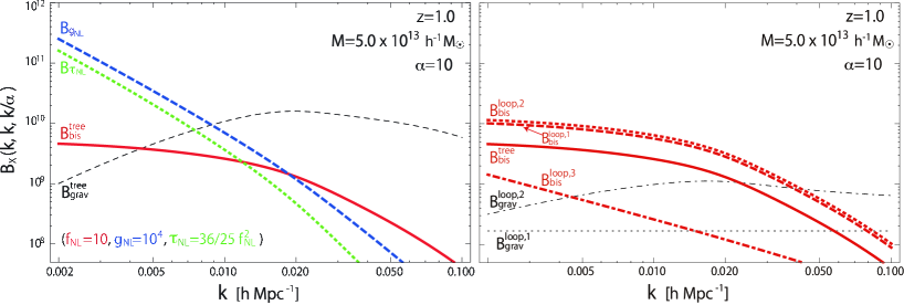
Figure 3: Left panel: Contributions $B_{\rm grav}^{\rm tree}$ (black thin dashed line), $B_{\rm bis}^{\rm tree}$ (red thick line), $B_{g_{\rm NL}}$ (blue thick dashed line), and $B_{\tau_{\rm NL}}$ (green thick dotted line), as functions of the wavenumber $k$ with $\alpha=10$. Right panel: One-loop contributions $B_{\rm grav}^{{\rm loop},1}$ (black thin dotted line), $B_{\rm grav}^{{\rm loop},2}$ (black thin dot-dashed line), $B_{\rm bis}^{{\rm loop},1}$ (red thick dashed line), $B_{\rm bis}^{{\rm loop},2}$ (red thick dotted line), $B_{\rm bis}^{{\rm loop},3}$ (red thick dot-dashed line), and $B_{\rm bis}^{\rm tree}$ (red thick line), as functions of the wavenumber $k$ with $\alpha=10$. Here, we fix the redshift and the mass scale of halos to $z=1.0$ and $M=5\times 10^{13}h^{-1}M_{\odot}$, respectively. The non-linearity parameters are given by $f_{\rm NL}=10$, $g_{\rm NL}=10^{4}$ and $\tau_{\rm NL}=36f_{\rm NL}^{2}/25$.

Right panel of Fig. 3 shows the one-loop contributions, $B_{\rm grav}^{{\rm loop},1}$ (black thin dotted line), $B_{\rm grav}^{{\rm loop},2}$ (black thin dot-dashed line), $B_{\rm bis}^{{\rm loop},1}$ (red thick dashed line), $B_{\rm bis}^{{\rm loop},2}$ (red thick dotted line), $B_{\rm bis}^{{\rm loop},3}$ (red thick dot-dashed line), and $B_{\rm bis}^{\rm tree}$ (red thick line). The results are again plotted as function of the wavenumber $k$ with $\alpha=10$. The one-loop contributions, $B_{\rm bis}^{{\rm loop},1}$ and $B_{\rm bis}^{{\rm loop},2}$, dominate the tree-level contribution, $B_{\rm bis}^{\rm tree}$. This fact has been also addressed by Jeong and Komatsu (2009) Jeong:2009vd , who computed the halo bispectrum on the basis of the peak formalism, taking account of the contribution from the primordial trispectrum.

The reason why the contributions $B_{\rm bis}^{{\rm loop},1}$ and $B_{\rm bis}^{{\rm loop},2}$ become larger than the other one-loop contributions may be explained from the diagrams shown in Fig. 1. Although all the diagrams in iPT are irreducible, the diagram of $B_{\rm bis}^{{\rm loop},3}$ graphically looks similar to $B_{\rm bis}^{\rm tree}$, and connecting two of the three grey circles with linear power spectrum gives $B_{\rm bis}^{{\rm loop},3}$. In similar way, $B_{\rm grav}^{{\rm loop},1}$ and $B_{\rm grav}^{{\rm loop},2}$ can be constructed from the tree diagram $B_{\rm grav}^{\rm tree}$ by adding a power spectrum. We may call them decomposable diagrams. On the other hand, the diagrams $B_{\rm bis}^{{\rm loop},1}$ and $B_{\rm bis}^{{\rm loop},2}$ can not be constructed from the tree diagrams by simply adding a power spectrum. We may call such kind of contributions un-decomposable diagrams. The un-decomposable diagrams in nature involve higher-order correlators of the initial linear density field, and these correlators form a specific type of loops by glueing some of the legs (indicated by solid lines) to a multi-point propagator. In the large-scale limit, their loop integral can be dominated by the contributions of the squeezed limit of the higher-order correlators. Since the local-type non-Gaussianity is known to produce a large primordial bispectrum in the squeezed limit, the un-decomposable diagram can potentially give a significantly large contribution to the halo bispectrum. Indeed, the expressions of $B_{\rm bis}^{{\rm loop},1}$ and $B_{\rm bis}^{{\rm loop},2}$ in the large-scale limit, given in Eq. (84), are mostly dominated by the squeezed limit of $B_{\rm L}$, and the effect of a strong coupling between short- and long-modes results in both the scale-dependence proportional to $\mathcal{M}(k)^{-1}\propto k^{-2}$ and the integral retaining the short-mode contribution that produces a very large amplitude.

Finally, in Fig. 4, we compare the total contribution from the gravitational non-linearity with those from primordial non-Gaussianity. Plotted results are the contributions $B_{\rm grav}(=B_{\rm grav}^{\rm tree}+B_{\rm grav}^{{\rm loop},1}+B_{\rm grav}^{{\rm loop},2})$ (black thin dashed line), $B_{\rm bis}(=B_{\rm bis}^{\rm tree}+B_{\rm bis}^{{\rm loop},1}+B_{\rm bis}^{{\rm loop},2}+B_{\rm bis}^{{\rm loop},3})$ (red thick line), $B_{g_{\rm NL}}$ (blue thick line), and $B_{\tau_{\rm NL}}$ (green thick line), as functions of $\alpha$, fixing the wavenumber to $k=0.007\,h\,{\rm Mpc}^{-1}$. As we saw before, the contributions from the primordial non-Gaussianity become large as increasing $\alpha$, and eventually dominate the halo bispectrum. In particular, in the squeezed limit ($\alpha\gg 1$), the term $B_{\tau_{\rm NL}}$ is found to exceed other non-Gaussian contributions.

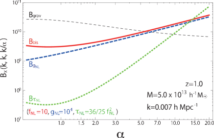
Figure 4: Contributions $B_{\rm grav}(=B_{\rm grav}^{\rm tree}+B_{\rm grav}^{{\rm loop},1}+B_{\rm grav}^{{\rm loop},2})$ (black thin dashed line), $B_{\rm bis}(=B_{\rm bis}^{\rm tree}+B_{\rm bis}^{{\rm loop},1}+B_{\rm bis}^{{\rm loop},2}+B_{\rm bis}^{{\rm loop},3})$ (red thick line), $B_{g_{\rm NL}}$ (blue thick line), and $B_{\tau_{\rm NL}}$ (green thick line), as functions of $\alpha$ with $k=0.007\,h\,{\rm Mpc}^{-1}$. Here, we fix that the redshift $z=1.0$ and the mass scale of halos $M=5\times 10^{13}h^{-1}M_{\odot}$. The non-linearity parameters are given by $f_{\rm NL}=10$, $g_{\rm NL}=10^{4}$ and $\tau_{\rm NL}=36f_{\rm NL}^{2}/25$.

III.2 Equilateral-type non-Gaussianity

Let us next consider the equilateral-type non-Gaussianity, in which the bispectrum of linear density field $B_{\rm L}$ is given by

$$B_{\rm L}({\bf k}_{1},{\bf k}_{2},{\bf k}_{3}) = 6f_{\rm NL}^{\rm equil}{\cal M}(k_{1}){\cal M}(k_{2}){\cal M}(k_{3})\left[-\left(P_{\Phi}(k_{1})P_{\Phi}(k_{2})+2~{}{\rm perms.}\right)\right.$$ (89)

$$\left.-2P_{\Phi}(k_{1})^{2/3}P_{\Phi}(k_{2})^{2/3}P_{\Phi}(k_{3})^{2/3}+\left(P_{\Phi}(k_{1})^{1/3}P_{\Phi}(k_{2})^{2/3}P_{\Phi}(k_{3})+5~{}{\rm perms.}\right)\right].$$

Here, we do not consider the contribution from the ”equilateral”-trispectrum, because its scale dependence strongly depends on the models of generating primordial non-Gaussianity. Also, its exact form is much complicated compared to that of the local-type non-Gaussianity. In fact, there are several works on the estimator for the trispectrum for the CMB temperature fluctuations in the models producing the equilateral-type bispectrum Mizuno:2010by ; Izumi:2011di . We leave the discussion on the contribution from the equilateral-trispectrum to future work.

The tree-level contribution from the primordial bispectrum, $B_{\rm bis}^{\rm tree}$, becomes

$$B_{\rm bis}^{\rm tree} = 6f_{\rm NL}^{\rm equil}\Gamma_{X}^{(1)}({\bf k}_{1})\Gamma_{X}^{(1)}({\bf k}_{2})\Gamma_{X}^{(1)}({\bf k}_{3}){\cal M}(k_{1}){\cal M}(k_{2}){\cal M}(k_{3})\left[-\left(P_{\Phi}(k_{1})P_{\Phi}(k_{2})+2~{}{\rm perms.}\right)\right.$$ (92)

$$\left.-2P_{\Phi}(k_{1})^{2/3}P_{\Phi}(k_{2})^{2/3}P_{\Phi}(k_{3})^{2/3}+\left(P_{\Phi}(k_{1})^{1/3}P_{\Phi}(k_{2})^{2/3}P_{\Phi}(k_{3})+5~{}{\rm perms.}\right)\right].$$

On the other hand, the one-loop contributions, $B_{\rm bis}^{{\rm loop},1}$ and $B_{\rm bis}^{{\rm loop},2}$ include the primordial bispectrum of the specific configuration, $B_{\rm L}({\bf k}_{i},-{\bf p},-{\bf k}_{i}+{\bf p})$. In the large-scale limit $k_{i}/p\ll 1$, the leading-order behavior becomes

$$B_{\rm L}({\bf k}_{i},-{\bf p},-{\bf k}_{i}+{\bf p})\approx 12f_{\rm NL}^{\rm equil}{P_{\rm L}(k_{i})\over{\cal M}(k_{i})}P_{\rm L}(p)\left({k_{i}\over p}\right)^{2}\left[\left({k_{i}\over p}\right)^{-{2\over 3}(n_{s}-1)}-\left({n_{s}-4\over 3}\right)^{2}\mu_{i}^{2}\right].$$ (93)

Here $\mu_{i}\equiv{{\bf k}_{i}\cdot{\bf p}\over k_{i}p}$ and we assume the power-law spectrum, $P_{\Phi}(k)\propto k^{n_{s}-4}$. Also, $B_{\rm bis}^{{\rm loop},3}$ has the primordial bispectrum of the configuration, $B_{\rm L}({\bf k}_{1},{\bf k}_{2}+{\bf p},{\bf k}_{3}-{\bf p})$, which can be reduced to

$$B_{\rm L}({\bf k}_{1},{\bf k}_{2}+{\bf p},{\bf k}_{3}-{\bf p})\approx 12f_{\rm NL}^{\rm equil}{P_{\rm L}(k_{1})\over{\cal M}(k_{1})}P_{\rm L}(p)\left({k_{1}\over p}\right)^{2}\left[\left({k_{1}\over p}\right)^{-{2\over 3}(n_{s}-1)}-\left({n_{s}-4\over 3}\right)^{2}\left({k_{2}^{2}\mu_{2}^{2}+k_{3}^{2}\mu_{3}^{2}\over k_{1}^{2}}\right)\right].$$ (94)

Then, we obtain the scale-dependence for the halo bispectrum induced from the equilateral primordial non-Gaussianity. In the large scale limit, we have

$$B_{\rm bis}^{\rm tree}\propto k^{0}\left({2\alpha-1\over\alpha^{2}}\right),~{}B_{\rm bis}^{{\rm loop},1}\propto k^{2}\alpha^{0},~{}B_{\rm bis}^{{\rm loop},2}\propto k^{2}\alpha^{0},~{}B_{\rm bis}^{{\rm loop},3}\propto k^{1}\alpha^{1}.$$ (95)

Here we simply assume the scale-invariant primordial power spectrum, that is, $n_{s}=1$. Because of the positive powers of $k$, the one-loop contributions from the equilateral-type bispectrum are all suppressed on the large scales, compared to the tree-level contribution.

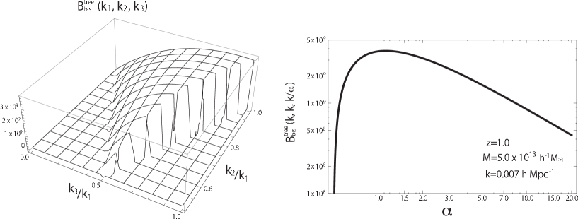
Figure 5: $B_{\rm bis}^{\rm tree}(k_{1},k_{2},k_{3})$ as function of $k_{3}/k_{1}$ and $k_{2}/k_{1}$ for $k_{1}=0.007\,h\,{\rm Mpc}^{-1}$ (left panel), and $B_{\rm bis}^{\rm tree}(k_{1},k_{2},k_{3})$ as a function of $\alpha$ with fixing $k=0.007\,h\,{\rm Mpc}^{-1}$ (right panel) for equilateral-type primordial non-Gaussianity. We take $f_{\rm NL}^{\rm equil}=100$.

Left panel of Fig. 5 shows the shape of $B_{\rm bis}^{\rm tree}(k_{1},k_{2},k_{3})$ in the momentum space, fixing wavenumber $k_{1}$ to $0.007\,h\,{\rm Mpc}^{-1}$, and we assume $k_{1}\geq k_{2}\geq k_{3}$ and $k_{3}\geq k_{1}-k_{2}$ because of the triangle condition. Right panel of Fig. 5 shows the $\alpha$-dependence of $B_{\rm bis}^{\rm tree}(k_{1},k_{2},k_{3})$, for isosceles configuration as $k_{1}=k_{2}=\alpha k_{3}=k$, and we fix the wavenumber $k$ to $0.007\,h\,{\rm Mpc}^{-1}$ and take $f_{\rm NL}^{\rm equil}=100$, which is almost the $2$-$\sigma$ upper bound obtained by Planck collaboration Ade:2013ydc . The amplitude of $B_{\rm bis}^{\rm tree}$ has a peak around $\alpha=1.0$, indicating that the halo bispectrum has equilateral shape in $k_{1},k_{2},k_{3}$ space. Since the contribution from the non-linearity of the gravitational evolution $B_{\rm grav}^{\rm tree}$ also has a peak around $\alpha=1.0$ (see Fig. 2), it seems difficult to distinguish between $B_{\rm bis}^{\rm tree}$ and $B_{\rm grav}^{\rm tree}$ in the case of equilateral-type non-Gaussianity.

However, the $k$-dependence of $B_{\rm bis}^{\rm tree}$ and $B_{\rm grav}^{\rm tree}$ has very distinct feature, as shown in Fig. 6. Here, we plot $B_{\rm grav}^{\rm tree}$ (black dashed line) and $B_{\rm bis}^{\rm tree}$ (red thick line) as a function of $k$, fixing $\alpha$ to unity and taking $f_{\rm NL}^{\rm equil}=100$. For the non-linearity parameter consistent with the current observational limit, we find that $B_{\rm bis}^{\rm tree}$ dominates $B_{\rm grav}^{\rm tree}$ at $k\lesssim 0.003\,h\,{\rm Mpc}^{-1}$. Note that the detectability of the equilateral primordial no-Gaussianity from galaxy survey has been discussed in Ref. Sefusatti:2007ih , which also found the similar scale-dependent behavior. The authors of Ref. Sefusatti:2007ih computed the galaxy bispectrum based on the local bias ansatz. At the tree level, the difference between our formula and the expression in Ref. Sefusatti:2007ih appears in the scale dependence of the term, $(1+{{\bf k}_{1}\cdot{\bf k}_{2}}/k_{1}^{2})c_{2}^{\rm L}$ included in $\Gamma_{X}^{(2)}({\bf k}_{1},{\bf k}_{2})$. This basically comes from the bias prescription which we adopted here Matsubara:2011ck ; Matsubara:2013ofa , and reflects the non-local nature of the halo bias, but it does not produce much difference in the halo bispectrum on large scales.

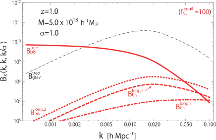
Figure 6: $B_{\rm grav}^{\rm tree}$ (black dashed line), $B_{\rm bis}^{\rm tree}$ (red thick line), $B_{\rm bis}^{{\rm loop},1}$ (red dashed thick line), $B_{\rm bis}^{{\rm loop},2}$ (red dotted thick line), and $B_{\rm bis}^{{\rm loop},3}$ (red dotted-dashed thick line) as a function of $k$ with fixing $\alpha=1.0$ for equilateral-type primordial non-Gaussianity. We take $f_{\rm NL}^{\rm equil}=100$.

In Fig. 6, we also plot the one-loop contributions for the equilateral-type; $B_{\rm grav}^{\rm tree}$ (black dashed line), $B_{\rm bis}^{\rm tree}$ (red thick line), $B_{\rm bis}^{{\rm loop},1}$ (red dashed thick line), $B_{\rm bis}^{{\rm loop},2}$ (red dotted thick line), and $B_{\rm bis}^{{\rm loop},3}$ (red dotted-dashed thick line). The one-loop contributions are all suppressed on large scales as mentioned before. In Ref. Sefusatti:2009qh , the one-loop corrections have been also discussed. The author computed the one-loop contributions with the Eulerian local bias prescription, and mentioned that one of the loop contributions is not negligible even for the equilateral-type non-Gaussianity. In the diagrammatic picture, this corresponds to the loop attached to an external vertex. In our formalism on the basis of iPT, however, such loops are already included in the multi-point propagator as a result of the resummation. Hence such higher-order loop corrections do not appear in our formula.

III.3 Orthogonal-type primordial non-Gaussianity

As the third type of primordial non-Gaussianity, we consider the orthogonal-type non-Gaussianity. The bispectrum of the orthogonal type is defined as

$$B_{\rm L}({\bf k}_{1},{\bf k}_{2},{\bf k}_{3}) = 6f_{\rm NL}^{\rm orth}{\cal M}(k_{1}){\cal M}(k_{2}){\cal M}(k_{3})\left[-3\left(P_{\Phi}(k_{1})P_{\Phi}(k_{2})+2~{}{\rm perms.}\right)\right.$$ (98)

$$\left.-8P_{\Phi}(k_{1})^{2/3}P_{\Phi}(k_{2})^{2/3}P_{\Phi}(k_{3})^{2/3}+3\left(P_{\Phi}(k_{1})^{1/3}P_{\Phi}(k_{2})^{2/3}P_{\Phi}(k_{3})+5~{}{\rm perms.}\right)\right].$$

Then we obtain

$$B_{\rm bis}^{\rm tree} = 6f_{\rm NL}^{\rm orth}\Gamma_{X}^{(1)}({\bf k}_{1})\Gamma_{X}^{(1)}({\bf k}_{2})\Gamma_{X}^{(1)}({\bf k}_{3}){\cal M}(k_{1}){\cal M}(k_{2}){\cal M}(k_{3})\left[-3\left(P_{\Phi}(k_{1})P_{\Phi}(k_{2})+2~{}{\rm perms.}\right)\right.$$ (101)

$$\left.-8P_{\Phi}(k_{1})^{2/3}P_{\Phi}(k_{2})^{2/3}P_{\Phi}(k_{3})^{2/3}+3\left(P_{\Phi}(k_{1})^{1/3}P_{\Phi}(k_{2})^{2/3}P_{\Phi}(k_{3})+5~{}{\rm perms.}\right)\right].$$

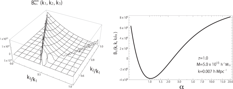
Figure 7: Left panel; $B_{\rm bis}^{\rm tree}(k_{1},k_{2},k_{3})$ as function of $k_{3}/k_{1}$ and $k_{2}/k_{1}$ for $k_{1}=0.007h{\rm Mpc}^{-1}$, Right panel; $B_{\rm bis}^{\rm tree}(k_{1},k_{2},k_{3})$ as a function of $\alpha$ with fixing $k=0.007h{\rm Mpc}^{-1}$, for orthogonal-type primordial non-Gaussianity. We take $f_{\rm NL}^{\rm orth}=-100$.

In Fig. 7, shape of the bispectrum $B_{\rm bis}^{\rm tree}(k_{1},k_{2},k_{3})$ (left) and its $\alpha$-dependence (right) are shown. For the parameter $f_{\rm NL}^{\rm orth}$, we adopt $f_{\rm NL}^{\rm orth}=-100$, consistent with the Planck results at $2$-$\sigma$ level Ade:2013ydc . Right panel shows as increasing $\alpha$, $B_{\rm bis}^{\rm tree}$ starts to decrease and has a negative peak around $\alpha=1.0$, and then turns to increase with positive value toward the squeezed limit ($\alpha\gg 1$). This is in marked contrast to the behaviors in other types of the non-Gaussianity, and may be a very important clue to separately detect the orthogonal-type non-Gaussianity from the halo bispectrum.

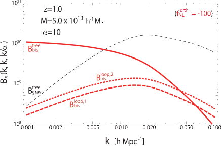
Figure 8: $B_{\rm grav}^{\rm tree}$ (black dashed line), $B_{\rm bis}^{\rm tree}$ (red thick line), $B_{\rm bis}^{{\rm loop},1}$ (red dashed thick line), and $B_{\rm bis}^{{\rm loop},2}$ (red dotted thick line) as a function of $k$ with fixing $\alpha=10$ for orthogonal-type primordial non-Gaussianity. We take $f_{\rm NL}^{\rm orth}=-100$.

Fig. 8 shows the scale-dependence of the halo bispectrum for the orthogonal type non-Gaussianity. In addition to the tree-level contributions, $B_{\rm grav}^{\rm tree}$ (black dashed line) and $B_{\rm bis}^{\rm tree}$ (red thick line), we also plot the one-loop contributions, $B_{\rm bis}^{{\rm loop},1}$ (red dashed thick line) and $B_{\rm bis}^{{\rm loop},2}$ (red dotted thick line) as functions of $k$, fixing $\alpha$ to $10$ and taking $f_{\rm NL}^{\rm orth}=-100$. Here, we do not show the contribution $B_{\rm bis}^{{\rm loop},3}$, because it turns out to be very small. As in the case of equilateral-type non-Gaussianity, the one-loop contributions are much suppressed, and tree-level contributions $B_{\rm bis}^{\rm tree}$ becomes dominant on very large-scales.

III.4 Comparison of total halo bispectrum between three types of primordial non-Gaussianity

Finally, let us compare the overall trend of the total halo bispectrum at the one-loop order between three-types of primordial non-Gaussianity. Fig. 9 shows the total halo bispectrum, $B_{X}(k,k,k/\alpha)$, as function of wavenumber, fixing $\alpha$ to $10$ (left) and $1.0$ (right). While upper panels present the results for the local-type non-Gaussianity with two different parameter set, i.e., $(f_{\rm NL},\,g_{\rm NL})=(10,\,0)$ and $(0,\,10^{4})$, bottom panels plot the halo bispectra for the equilateral- (green) and orthogonal- types (magenta dashed). Here, we assume that the consistency relation, $\tau_{\rm NL}=36f_{\rm NL}^{2}/25$, strictly holds for local-type non-Gaussianity. In each panel, black solid line indicates the result in the absence of the primordial non-Gaussianity, and considers only the contributions from the gravitational non-linearity.

For the non-linearity parameters consistent with current observations, the local-type non-Gaussianity gives the largest signal of the halo bispectrum in the squeezed case at large-scale. A notable point is that even with $\alpha=1.0$, a strong enhancement of the amplitude of bispectrum can be observed, especially in the case of $(f_{\rm NL},\,g_{\rm NL})=(0,\,10^{4})$. The scale-dependence of the halo bispectrum also appears in the cases of the equilateral- and orthogonal-type non-Gaussianities (see bottom panel). Although the effect is rather moderate, at large-scales, the contribution from primordial non-Gaussianity can exceed that from the gravitational non-linearity. Further, as we have seen in Sec. III.3, additionally interesting feature can be seen for the orthogonal-type non-Gaussianity. With a negative non-linearity parameter $f_{\rm NL}^{\rm orth}<0$, the sign of the halo bispectrum eventually flips at large scales for the configuration with $\alpha\sim 1$. This would be unique and important feature to distinguish the non-Gaussian signal from other types of non-Gaussianity.

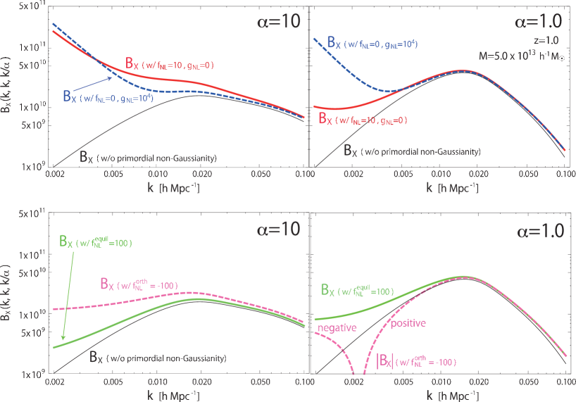
Figure 9: Upper panels: total halo bispectrum, $B_{X}(k,k,k/\alpha)$, for local-type with $\alpha=10$ (left) and $\alpha=1.0$ (right). Black thin line is for the case without any primordial non-Gaussianity, red thick line is for the case with $f_{\rm NL}=10$, $\tau_{\rm NL}=36f_{\rm NL}^{2}/25$ and $g_{\rm NL}=0$, and blue thick dashed line is for the case with $f_{\rm NL}=0$ and $g_{\rm NL}=10^{4}$. Lower panels: total halo bispectrum, $B_{X}(k,k,k/\alpha)$, for equilateral- (green thick line) and orthogonal-types (magenta thick dashed line) with $\alpha=10$ (left) and $\alpha=1.0$ (right). We fix the non-linearity parameters to $f_{\rm NL}^{\rm equil}=100$ and $f_{\rm NL}^{\rm orth}=-100$. In all panels, we fix the redshift and the mass of halos to $z=1.0$ and $M=5\times 10^{13}h^{-1}M_{\odot}$.

IV Impact of higher-order contributions

In the formalism of iPT, the contribution from the primordial non-Gaussianity on the halo bispectrum can be efficiently estimated from the diagrams including the linear (primordial) polyspectra. Increasing the order of perturbations, we can systematically calculate the contributions from higher-order polyspectra. Naively, we expect that higher-loop contributions are generally suppressed on very large scales. As we saw in Sec. III.1, however, one-loop contributions from the local-type non-Gaussianity are found to be non-negligible on large scales, and can eventually dominate the tree-level contributions. This partly implies that the perturbative treatment may not work well in the case of local-type non-Gaussianity, and the contribution from the two-loop order would be also dominant. In this section, focusing on the local-type non-Gaussianity, we study the impact of two-loop contribution on the halo bispectrum.

IV.1 Two-loop contributions from the primordial trispectrum

As we found in Sec. III.1, non-negligible contributions coming from the one-loop corrections are described by the un-decomposable diagrams, which can not be simply constructed from tree-level diagrams by adding a primordial power spectrum (shown in Fig. 1). In this respect, at two-loop order, possible non-negligible contributions may come from the diagrams linearly proportional to the primordial trispectrum or quadratically proportional to the primordial bispectrum. The other contributions linearly proportional to the primordial bispectrum would be certainly suppressed, since they are described as decomposable diagrams.

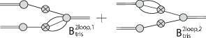
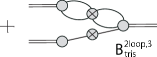
Figure 10: Two loop diagrams linearly proportional to the primordial trispectrum.

Let us first consider the two-loop un-decomposable contributions linearly proportional to the primordial trispectrum. The corresponding diagrams are shown in Fig. 10, each of which are analytically expressed as

$$B_{\rm tris}^{2{\rm loop},1} = {1\over 6}\Biggl{[}\Gamma_{X}^{(1)}({\bf k}_{1})\Gamma_{X}^{(1)}({\bf k}_{2})P_{\rm L}(k_{1})$$ (104)

$$\quad\times\int{d^{3}p_{1}d^{3}p_{2}\over(2\pi)^{6}}\Gamma_{X}^{(4)}(-{\bf k}_{1},{\bf p}_{1},{\bf p}_{2},-{\bf k}_{2}-{\bf p}_{1}-{\bf p}_{2})T_{\rm L}({\bf k}_{2},{\bf p}_{1},{\bf p}_{2},-{\bf k}_{2}-{\bf p}_{1}-{\bf p}_{2})+5~{}{\rm perms.}\Biggr{]},$$

$$B_{\rm tris}^{2{\rm loop},2} = {1\over 6}\Biggl{[}\Gamma_{X}^{(1)}({\bf k}_{1})\Gamma_{X}^{(2)}(-{\bf k}_{1},-{\bf k}_{3})P_{\rm L}(k_{1})$$ (108)

$$\quad\times\int{d^{3}p_{1}d^{3}p_{2}\over(2\pi)^{6}}\Gamma_{X}^{(3)}({\bf p}_{1},{\bf p}_{2},{\bf k}_{3}-{\bf p}_{1}-{\bf p}_{2})T_{\rm L}(-{\bf k}_{3},{\bf p}_{1},{\bf p}_{2},{\bf k}_{3}-{\bf p}_{1}-{\bf p}_{2})+5~{}{\rm perms.}\Biggr{]},$$

$$B_{\rm tris}^{2{\rm loop},3} = {1\over 4}\Biggl{[}\Gamma_{X}^{(1)}({\bf k}_{1})P_{\rm L}(k_{1})\int{d^{3}p_{1}d^{3}p_{2}\over(2\pi)^{6}}\Gamma_{X}^{(2)}({\bf p}_{1},{\bf k}_{2}-{\bf p}_{1})$$ (112)

$$\qquad\qquad\qquad\times\Gamma_{X}^{(3)}({\bf k}_{1},{\bf p}_{2},-{\bf k}_{2}-{\bf p}_{2})T_{\rm L}({\bf p}_{1},{\bf k}_{2}-{\bf p}_{1},{\bf p}_{2},-{\bf k}_{2}-{\bf p}_{2})+5~{}{\rm perms.}\Biggr{]}.$$

In a manner similar to what we did in Sec. III.1, we take the large-scale limit, $k_{i}\to 0$. Then, we have

$$B_{\rm tris}^{2{\rm loop},1} \approx \left(3g_{\rm NL}+{25\over 9}\tau_{\rm NL}\right)\Gamma_{X}^{(1)}({\bf k}_{1})\Gamma_{X}^{(1)}({\bf k}_{2})P_{\rm L}(k_{1}){P_{\rm L}(k_{2})\over{\cal M}(k_{2})}\int{d^{3}p_{1}d^{3}p_{2}\over(2\pi)^{6}}\Bigl{[}-{{\bf k}_{1}\cdot{\bf k}_{3}\over k_{1}^{2}}c_{3}^{\rm L}({\bf p}_{1},{\bf p}_{2},-{\bf p}_{1}-{\bf p}_{2})$$ (115)

$$\qquad\qquad\quad+c_{4}^{\rm L}(-{\bf k}_{1},{\bf p}_{1},{\bf p}_{2},-{\bf p}_{1}-{\bf p}_{2})\Bigr{]}{\cal M}(p_{1}){\cal M}(p_{2}){\cal M}(|{\bf p}_{1}+{\bf p}_{2}|)P_{\Phi}(p_{1})P_{\Phi}(p_{2})+5~{}{\rm perms.},$$

$$B_{\rm tris}^{2{\rm loop},2} \approx \left(3g_{\rm NL}+{25\over 9}\tau_{\rm NL}\right)\Gamma_{X}^{(1)}({\bf k}_{1})\Gamma_{X}^{(2)}(-{\bf k}_{1},-{\bf k}_{3})P_{\rm L}(k_{1}){P_{\rm L}(k_{3})\over{\cal M}(k_{3})}$$ (119)

$$\qquad\times\int{d^{3}p_{1}d^{3}p_{2}\over(2\pi)^{6}}c_{3}^{\rm L}({\bf p}_{1},{\bf p}_{2},-{\bf p}_{1}-{\bf p}_{2}){\cal M}(p_{1}){\cal M}(p_{2}){\cal M}(|{\bf p}_{1}+{\bf p}_{2}|)P_{\Phi}(p_{1})P_{\Phi}(p_{2})+5~{}{\rm perms.},$$

$$B_{\rm tris}^{2{\rm loop},3} \approx 3g_{\rm NL}\Gamma_{X}^{(1)}({\bf k}_{1})P_{\rm L}(k_{1})\Biggl{\{}\int{d^{3}p_{1}\over(2\pi)^{3}}c_{2}^{\rm L}({\bf p}_{1},-{\bf p}_{1})P_{\rm L}(p_{1})$$ (131)

$$\qquad\qquad\times\int{d^{3}p_{2}\over(2\pi)^{3}}\left[-{{\bf k}_{1}\cdot{\bf k}_{3}\over k_{1}^{2}}c_{2}^{\rm L}({\bf p}_{2},-{\bf p}_{2})+c_{3}^{\rm L}(-{\bf k}_{1},{\bf p}_{2},-{\bf p}_{2})\right]P_{\rm L}(p_{2})P_{\Phi}(p_{2})$$

$$+\int{d^{3}p_{1}\over(2\pi)^{3}}c_{2}^{\rm L}({\bf p}_{1},-{\bf p}_{1})P_{\rm L}(p_{1})P_{\Phi}(p_{1})$$

$$\qquad\qquad\times\int{d^{3}p_{2}\over(2\pi)^{3}}\left[-{{\bf k}_{1}\cdot{\bf k}_{3}\over k_{1}^{2}}c_{2}^{\rm L}({\bf p}_{2},-{\bf p}_{2})+c_{3}^{\rm L}(-{\bf k}_{1},{\bf p}_{2},-{\bf p}_{2})\right]P_{\rm L}(p_{2})\Biggr{\}}+5~{}{\rm perms.}$$

$$+{25\over 9}\tau_{\rm NL}\Gamma_{X}^{(1)}({\bf k}_{1})P_{\rm L}(k_{1}){P_{\rm L}(k_{2})\over{\cal M}(k_{2})^{2}}\int{d^{3}p_{1}\over(2\pi)^{3}}c_{2}^{\rm L}({\bf p}_{1},-{\bf p}_{1})P_{\rm L}(p_{1})$$

$$\qquad\qquad\times\int{d^{3}p_{2}\over(2\pi)^{3}}\left[-{{\bf k}_{1}\cdot{\bf k}_{3}\over k_{1}^{2}}c_{2}^{\rm L}({\bf p}_{2},-{\bf p}_{2})+c_{3}^{\rm L}(-{\bf k}_{1},{\bf p}_{2},-{\bf p}_{2})\right]P_{\rm L}(p_{2})+5~{}{\rm perms.}.$$

Here, we used the fact that

$$\Gamma^{(4)}_{X}(-{\bf k}_{1},{\bf p}_{1},{\bf p}_{2},-{\bf k}_{2}-{\bf p}_{1}-{\bf p}_{2})\approx-{{\bf k}_{1}\cdot{\bf k}_{3}\over k_{1}^{2}}c_{3}^{\rm L}({\bf p}_{1},{\bf p}_{2},-{\bf p}_{1}-{\bf p}_{2})+c_{4}^{\rm L}(-{\bf k}_{1},{\bf p}_{1},{\bf p}_{2},-{\bf p}_{1}-{\bf p}_{2}).$$ (132)

From the above expressions, we find

$$B_{\rm tris}^{2{\rm loop},1}\propto k^{0}\alpha^{1},~{}B_{\rm tris}^{2{\rm loop},2}\propto k^{0}\alpha^{1},~{}B_{\rm tris}^{2{\rm loop},3}\propto k^{-2}\alpha^{3}~{}.$$ (133)

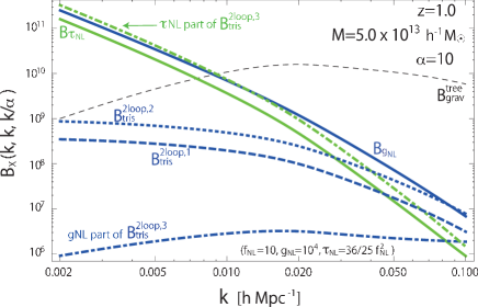
Figure 11: Two-loop contributions from the primordial trispectrum are plotted, which are $B_{\rm tris}^{2{\rm loop},1}$ (blue dashed thick line), $B_{\rm tris}^{2{\rm loop},2}$ (blue dotted thick line), $g_{\rm NL}$ contribution in $B_{\rm tris}^{2{\rm loop},3}$ (blue dot-dashed thick line), and $\tau_{\rm NL}$ contribution in $B_{\rm tris}^{2{\rm loop},3}$ (green dot-dashed thick line), as functions of $k$. We also plot $B_{\rm grav}^{\rm tree}$ (black dashed line), $B_{g_{\rm NL}}$ (blue thick line), and $B_{\tau_{\rm NL}}$ (green thick line) as references. We take $g_{\rm NL}=10^{4}$ and $\tau_{\rm NL}=(36/25)10^{2}$ and fix the redshift, the mass of halos and the squeezing parameter to $z=1.0$, $M=5\times 10^{13}h^{-1}M_{\odot}$, and $\alpha=10$.

In Fig. 11, the three two-loop contributions, $B_{\rm tris}^{2{\rm loop},1}$ (blue dashed thick line), $B_{\rm tris}^{2{\rm loop},2}$ (blue dotted thick line), and $B_{\rm tris}^{2{\rm loop},3}$, are plotted as functions of $k$, fixing $\alpha$ to $10$. For the contribution, $B_{\rm tris}^{2{\rm loop},3}$, we divide it into two pieces, and separately show the contributions proportional to $g_{\rm NL}$ (blue dot-dashed thick line) and $\tau_{\rm NL}$ (green dot-dashed thick line). Then, all the un-decomposable two-loop contributions proportional to $g_{\rm NL}$ turn out to be sub-dominant on large scales, while the term proportional to $\tau_{\rm NL}$ (labeled as $\tau_{\rm NL}$ part of $B_{\rm tris}^{2{\rm loop},3}$) gives a significantly large contribution, which can dominate over the one-loop contribution, $B_{\tau_{\rm NL}}$. This implies that we need to develop at least the two-loop order calculations if one wants to evaluate the contribution of the halo bispectrum linearly proportional to the non-linearity parameter $\tau_{\rm NL}$. As for the case of $g_{\rm NL}$, the one-loop order calculation seems sufficient on large scales.

IV.2 Other two-loop contributions

Consider next the un-decomposable two-loop contributions quadratically proportional to the primordial bispectrum, which are diagrammatically shown in Fig. 12. For local-type non-Gaussianity, the inequality, $\tau_{\rm NL}\geq 36f_{\rm NL}^{2}/25$, generally holds. In the case of equality which we consider here, this implies that the diagrams of the $\mathcal{O}(f_{\rm NL}^{2})$ order are expected to give a significant contribution comparable to the $\tau_{\rm NL}$ contribution, and potentially become dominant on large scales.

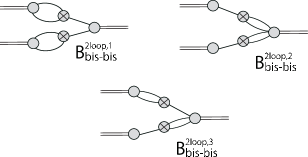
Figure 12: Undecomposable diagrams which are quadratically proportional to the primordial bispectrum.

In the large-scale limit, we approximately have

$$B_{\rm bis-bis}^{2{\rm loop},1} = {1\over 4}\Gamma_{X}^{(2)}({\bf k}_{1},{\bf k}_{2})\int{d^{3}p_{1}d^{3}p_{2}\over(2\pi)^{6}}\Gamma_{X}^{(2)}({\bf p}_{1},{\bf k}_{1}-{\bf p}_{1})\Gamma_{X}^{(2)}({\bf p}_{2},{\bf k}_{2}-{\bf p}_{2})$$ (136)

$$\qquad\qquad\qquad\times B_{\rm L}(-{\bf k}_{1},{\bf p}_{1},{\bf k}_{1}-{\bf p}_{1})B_{\rm L}(-{\bf k}_{2},{\bf p}_{2},{\bf k}_{2}-{\bf p}_{2})+2~{}{\rm perms.}$$

$$\approx 4f_{\rm NL}^{2}\Gamma_{X}^{(2)}({\bf k}_{1},{\bf k}_{2}){P_{\rm L}(k_{1})P_{\rm L}(k_{2})\over{\cal M}(k_{1}){\cal M}(k_{2})}\left[\int{d^{3}p\over(2\pi)^{3}}c_{2}^{\rm L}({\bf p},-{\bf p})P_{\rm L}(p)\right]^{2}+2~{}{\rm perms.},$$ (138)

$$B_{\rm bis-bis}^{2{\rm loop},2} \approx 4f_{\rm NL}^{2}\Gamma_{X}^{(1)}({\bf k}_{1})\Gamma_{X}^{(1)}({\bf k}_{2})\int{d^{3}p_{1}d^{3}p_{2}\over(2\pi)^{6}}c_{4}^{\rm L}({\bf p}_{1},-{\bf p}_{1},{\bf p}_{2},-{\bf p}_{2})P_{\rm L}(p_{1})P_{\rm L}(p_{2}){P_{\rm L}(k_{1})P_{\rm L}(k_{2})\over{\cal M}(k_{1}){\cal M}(k_{2})}+2~{}{\rm perms.},$$ (140)

$$B_{\rm bis-bis}^{2{\rm loop},3} \approx 4f_{\rm NL}^{2}\Gamma_{X}^{(1)}({\bf k}_{1}){P_{\rm L}(k_{1})P_{\rm L}(k_{2})\over{\cal M}(k_{1}){\cal M}(k_{2})}\int{d^{3}p_{1}\over(2\pi)^{3}}c_{2}^{\rm L}({\bf p}_{1},-{\bf p}_{1})P_{\rm L}(p_{1})$$ (144)

$$\times\int{d^{3}p_{2}\over(2\pi)^{3}}\left[-{{\bf k}_{2}\cdot{\bf k}_{3}\over k_{2}^{2}}c_{2}^{\rm L}(-{\bf p}_{2},{\bf p}_{2})+c_{3}^{\rm L}(-{\bf k}_{2},-{\bf p}_{2},{\bf k}_{1}+{\bf p}_{2})\right]P_{\rm L}(p_{2})+5~{}{\rm perms.}~{}.$$

Then, the asymptotic behavior of these contributions becomes

$$B_{\rm bis-bis}^{2{\rm loop},1}\propto k^{-2}\alpha~{},~{}B_{\rm bis-bis}^{2{\rm loop},2}\propto k^{-2}\alpha~{},~{}B_{\rm bis-bis}^{2{\rm loop},3}\propto k^{-2}\alpha~{}.$$ (145)

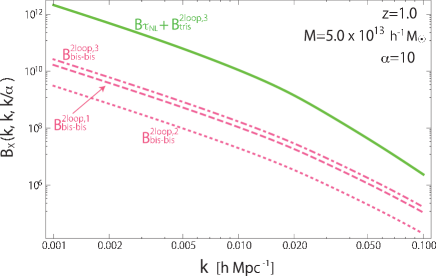
Figure 13: $B_{\tau_{\rm NL}}(k,k,k/\alpha)+B_{\rm tris}^{2{\rm loop},3}(k,k,k/\alpha)$ (green thick line), $B_{\rm bis-bis}^{2{\rm loop},1}$ (magenta dashed line), $B_{\rm bis-bis}^{2{\rm loop},2}$ (magenta dotted line), and $B_{\rm bis-bis}^{2{\rm loop},3}$ (magenta dot-dashed line) as a function of $k$ with fixing $\alpha=10$. We take $f_{\rm NL}^{\rm local}=10$ and $\tau_{\rm NL}=36f_{\rm NL}^{2}/25$.

In Fig. 13, the two-loop contributions given above are plotted as functions of $k$, fixing $\alpha$ to $10$; $B_{\rm bis-bis}^{2{\rm loop},1}$ (magenta dashed), $B_{\rm bis-bis}^{2{\rm loop},2}$ (magenta dotted), and $B_{\rm bis-bis}^{2{\rm loop},3}$ (magenta dot-dashed). For comparison, we also plot the one- and two-loop contributions linearly proportional to $\tau_{\rm NL}$, i.e., $B_{\tau_{\rm NL}}(k,k,k/\alpha)+B_{\rm tris}^{2{\rm loop},3}(k,k,k/\alpha)$ (green thick), assuming $f_{\rm NL}^{\rm local}=10$ and $\tau_{\rm NL}=36f_{\rm NL}^{2}/25$. Then, all the two-loop contributions quadratically proportional to the primordial bispectrum can become sub-dominant, and are well below the $\tau_{\rm NL}$-contribution. The asymptotic behaviors given in Eqs. (85), (133), and (145) indicate that all the contributions shown in Fig. 13 scale as $k^{-2}$, but the terms $B_{\tau_{\rm NL}}$ and $B_{\rm tris}^{2{\rm loop},3}$ have a larger power of $\alpha$, and are proportional to $\alpha^{3}$, which results in a significantly larger amplitude than that of $B_{\rm bis-bis}^{2{\rm loop}}$ by two orders of magnitude.

To sum up, it is not always the case that the higher loop contributions are suppressed compared with the lower loop contributions. In particular, the un-decomposable loop diagrams in the context of iPT would produce dominant contributions in the large-scale halo bispectrum, and hence we need to take into account all of the un-decomposable diagrams in order to precisely evaluate the effect of primordial non-Gaussianity on the halo bispectrum. In doing this, the diagrammatic approach based on the iPT helps us to systematically collect these dominant contributions.

V Discussion

In this section, we discuss several points which have not been yet clarified in previous sections. First, in Sec. V.1, we examine the dependence of redshift and halo mass on the halo bispectrum in the case of local-type non-Gaussianity. In Sec. V.2, to infer the asymptotic behavior of the bispectrum, we give a simple estimate of the scale-dependent behaviors using the diagrammatic approach. Finally, in Sec. V.3, the results of our analysis are compared with those of recent other works.

V.1 Dependence of redshift and mass of halos on the bispectrum

So far, we have set the redshift and the mass scale of halos to $z=1.0$ and $M=5\times 10^{13}h^{-1}M_{\odot}$ as representative values relevant for observations. Here, focusing on the local-type non-Gaussianity and based on the formulae for bispectrum at one-loop order, we discuss the redshift and the mass dependences of the halo bispectrum.

V.1.1 redshift

The redshift dependence of the halo bispectrum is shown in Fig. 14.

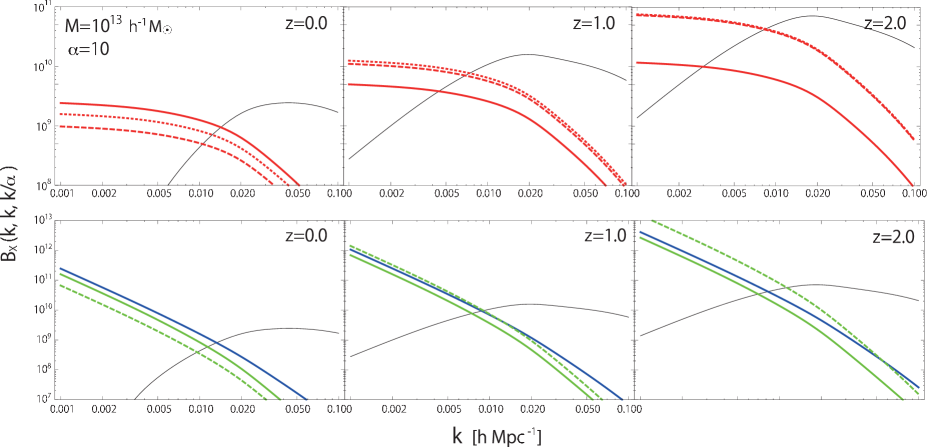
Figure 14: Each contribution of the halo bispectrum, Top - $B_{\rm grav}$ (black), $B_{\rm bis}^{\rm tree}$ (red thick), $B_{\rm bis}^{{\rm loop},1}$ (red thick dashed), and $B_{\rm bis}^{{\rm loop},2}$ (red thick dotted), Bottom - $B_{\rm grav}$ (black), $B_{g_{\rm NL}}$ (blue thick), $B_{\tau_{\rm NL}}$ (green thick), and $B_{\rm tris}^{2{\rm loop},3}$ (green thick dashed) with changing the mass of halo as $z=0.0$ (left), $z=1.0$ (central), and the right for $z=2.0$ (right).

In this figure, we plot each contribution of the halo bispectrum, $B_{\rm grav}$ (black), $B_{\rm bis}^{\rm tree}$ (red thick), $B_{\rm bis}^{{\rm loop},1}$ (red thick dashed), and $B_{\rm bis}^{{\rm loop},2}$ (red thick dotted) in top panels, and $B_{\rm grav}$ (black), $B_{g_{\rm NL}}$ (blue thick), $B_{\tau_{\rm NL}}$ (green thick), and $B_{\rm tris}^{2{\rm loop},3}$ (green thick dashed) in bottom panels. From left to right, we change the redshift as $z=0.0$, $1.0$, and $2.0$. For these redshifts, we have checked that the other contributions are also suppressed. From this figure, we find that the scale-dependence of the halo bispectrum does not change with the redshift, but the most dominant contribution changes. The redshift parameter has an affect on not only the evolution of the density perturbations but also $b_{n}^{\rm L}$. Basically, the density perturbations grow as the redshift parameter decreases. On the other hand, once the mass is fixed, the halo at the higher redshift becomes more highly biased object and it means larger value of $b_{n}^{\rm L}$. As shown in Fig. 14, the halo bispectrum becomes larger at the higher redshift and hence we find that the halo bispectrum seems to have the stronger dependence of the redshift parameter through $b_{n}^{\rm L}$ than the growth function $D(z)$. As for the most dominant contribution, we find for the more highly biased object the higher order loop contribution becomes important. Basically, the higher order loop contribution depends on the higher order scale-independent Lagrangian bias parameter $b_{n}^{\rm L}$ and such higher order $b_{n}^{\rm L}$ tends to become larger for the more highly biased object. Hence, the higher order loop contribution becomes important for the higher redshift, as can be seen in Fig. 14.

V.1.2 mass of the halos

The mass dependence of the halo bispectrum is shown in Fig. 15.

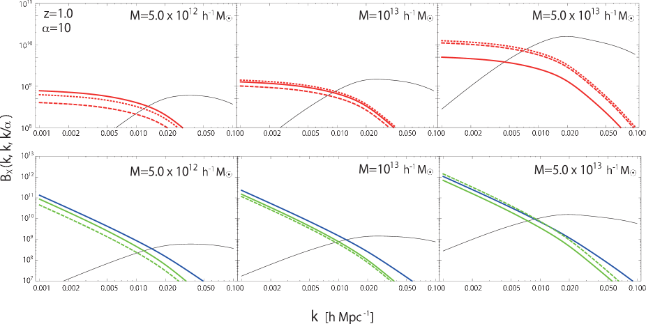
Figure 15: Each contribution of the halo bispectrum, Top - $B_{\rm grav}$ (black), $B_{\rm bis}^{\rm tree}$ (red thick), $B_{\rm bis}^{{\rm loop},1}$ (red thick dashed), and $B_{\rm bis}^{{\rm loop},2}$ (red thick dotted), Bottom - $B_{\rm grav}$ (black), $B_{g_{\rm NL}}$ (blue thick), $B_{\tau_{\rm NL}}$ (green thick), and $B_{\rm tris}^{2{\rm loop},3}$ (green thick dashed) with changing the mass of halo as $M=5.0\times 10^{12}h^{-1}M_{\odot}$ (left), $M=10^{13}h^{-1}M_{\odot}$ (central), and $M=5.0\times 10^{13}h^{-1}M_{\odot}$ (right).

In this figure, we plot each contribution of the halo bispectrum, $B_{\rm grav}$ (black), $B_{\rm bis}^{\rm tree}$ (red thick), $B_{\rm bis}^{{\rm loop},1}$ (red thick dashed), and $B_{\rm bis}^{{\rm loop},2}$ (red thick dotted) in top panels, and $B_{\rm grav}$ (black), $B_{g_{\rm NL}}$ (blue thick), $B_{\tau_{\rm NL}}$ (green thick), and $B_{\rm tris}^{2{\rm loop},3}$ (green thick dashed) in bottom panels. From left to right, we change the mass of halo as $M=5.0\times 10^{12}h^{-1}M_{\odot}$, $10^{13}h^{-1}M_{\odot}$, and $5.0\times 10^{13}h^{-1}M_{\odot}$. As in the discussion about the redshift dependence, we have checked that the other contributions are suppressed, and we also find that the scale-dependence of the halo bispectrum does not change with changing the mass of halo, but the dominant contribution changes. The dependence of the mass of halos is reflected in the scale-independent Lagrangian bias parameter $b_{n}^{\rm L}$, and it becomes larger for the larger mass. As we discussed before, higher order $b_{n}^{\rm L}$ tends to become larger for the larger mass and hence the higher order loop contribution becomes more important for the larger mass of the halos, as can be seen in Fig. 15.

As the result, although which loop contribution dominates in the halo bispectrum on large scales depends on the bias parameter $b_{n}^{\rm L}$, that is, the redshift and the mass of observed halos, we stress that it should be essential to consider both contributions of one and two-loops coming from the primordial trispectrum.

V.2 Asymptotic scale-dependence

The asymptotic scale-dependence is important to find dominant contributions of the halo bispectrum on large scales. In the discussion above, starting with the analytic expression of each diagram, we took the large-scale limit, and have finally derived the formulae for asymptotic scale-dependence. Here, we will argue that using the diagrammatic approach, these formulae can be recovered more easily and systematically.

First consider the simple case, and look at the contribution, $B_{\rm grav}^{\rm tree}$, shown in Fig. 1. This diagram can be graphically divided into two pieces, consisting of linear power spectrum of the biased object, $P_{X}^{\rm lin}$. Thus, we may write it as $B_{\rm grav}^{\rm tree}\propto P_{X}^{\rm lin}\times P_{X}^{\rm lin}$. For scale-invariant primordial fluctuations, the linear power spectrum $P_{X}^{\rm lin}$ is proportional to $k$ on large scales, and we immediately obtain $B_{\rm grav}^{\rm tree}(k_{1},k_{2},k_{3})\propto P_{X}^{\rm lin}(k_{1})\times P_{X}^{\rm lin}(k_{2})+2~{}{\rm perms.}\propto k^{2}\alpha^{0}$, as a dominant contribution on large scales ($k\to 0$) in the squeezed limit ($\alpha\to\infty$).

Similarly, we can also divide the contribution of the diagrams $B_{\rm bis}^{{\rm loop},1}$ and $B_{\rm bis}^{{\rm loop},2}$ in Fig. 1 into two pieces. In this case, a part of the diagram is $P_{X}^{\rm lin}$, but another piece corresponds to the one-loop power spectrum of the biased object, induced by the primordial bispectrum, $P_{X}^{\rm loop}$. It is known in the literature that the local-type primordial bispectrum generates a strong scale-dependence in the bias parameter, which scales as $k^{-2}$. In iPT, the main contribution of this indeed comes from the one-loop power spectrum, and we have $P_{X}^{\rm loop}\propto P_{X}^{\rm lin}/k^{2}\propto k^{-1}$. Hence, we reproduce the asymptotic scale-dependence of $B_{\rm bis}^{{\rm loop},1}$ and $B_{\rm bis}^{{\rm loop},2}$, and we obtain

$$B_{\rm bis}^{{\rm loop},1(2)}(k_{1},k_{2},k_{3})\propto P_{X}^{\rm lin}(k_{1})\times P_{X}^{\rm loop}(k_{2})+2~{}{\rm perms.}\propto k^{0}\alpha,$$

as a dominant contribution on large scales in the squeezed limit. This systematic approach based on the diagrammatic picture can also apply to the other contributions, and we easily find their asymptotic scale-dependences.

V.3 Comparison with other works

Finally, let us compare the results of our analysis with those of the recent works. In Ref. Jeong:2009vd , adopting the Taylor-expansion with local bias ansatz, the authors derived the formula for the halo bispectrum based on the Matarrese-Lucchin-Bonometto (MLB) formalism Matarrese:1986et . MLB formalism is nothing but the peak formalism, and we confirmed that taking the high-peak limit, our formula at the one-loop order reproduces the result in Ref. Jeong:2009vd . In the present paper, we further investigated the two-loop contribution, and found a new dominant contribution from the primordial trispectrum, which has not been considered in Ref. Jeong:2009vd .

As another analytic approach, Ref. Baldauf:2010vn has presented a formula for the halo bispectrum based on the peak-background split picture. The authors particularly examined the case of the single-component non-Gaussianity characterized by the curvature perturbation, $\Phi=\Phi_{G}+f_{\rm NL}(\Phi_{G}^{2}-\langle\Phi_{G}^{2}\rangle)+g_{\rm NL}\Phi_{G}^{3}$. Following Ref. Matsubara:2012nc , and using the cancellation properties of the highest-order parameters in Press-Schechter mass function, we have checked that our formula is consistent with Eq. (5.1) in Ref. Baldauf:2010vn in the large-scale limit. Note that the bispectrum formula in Ref. Baldauf:2010vn additionally includes contributions proportional to $f_{\rm NL}^{3}$ or $f_{\rm NL}^{4}$, for which we did not consider here. As shown in the figures in Ref. Baldauf:2010vn , however, these contributions can become significant only at very much large scales ($k\lesssim 0.002h{\rm Mpc}^{-1}$) in the squeezed isosceles configuration ($\alpha=10$). Ref. Nishimichi:2009fs investigated the halo bispectrum in cosmological $N$-body simulations, and found that the results of their simulations are rather consistent with those predicted by Ref. Jeong:2009vd , and the dominant contribution of bispectrum scales as $f_{\rm NL}^{2}$ in the squeezed limit. Hence, the contributions proportional to $f_{\rm NL}^{3}$ or $f_{\rm NL}^{4}$ might not be relevant for real observations.

Although we do not discuss in detail, we note here that these contributions can be also constructed in the formalism of the iPT. Such contributions come from the primordial higher-order poly-spectra as follows. For the single-sourced case, the primordial higher-order spectra can be simply parameterized by the non-linearity parameter $f_{\rm NL}$. For example, the primordial 5- and 6-point spectra respectively have the dependence of $f_{\rm NL}^{3}$ and $f_{\rm NL}^{4}$. Including such primordial higher-order poly-spectra and considering corresponding undecomposable diagrams, we can recover the same contributions as found in Ref. Baldauf:2010vn . We also find a crude relationship between the contributions from $\tau_{\rm NL}$ and that from $f_{\rm NL}^{3}$ and $f_{\rm NL}^{4}$ as $B_{f_{\rm NL}^{3}}\sim B_{\tau_{\rm NL}}\times(f_{\rm NL}/{\cal M}(k))$ and $B_{f_{\rm NL}^{4}}\sim B_{\tau_{\rm NL}}\times(f_{\rm NL}/{\cal M}(k))^{2}$, where we respectively denote the contributions from $f_{\rm NL}^{3}$ and $f_{\rm NL}^{4}$ as $B_{f_{\rm NL}^{3}}$ and $B_{f_{\rm NL}^{4}}$. From this relation, in order for $B_{f_{\rm NL}^{3}}$ and $B_{f_{\rm NL}^{4}}$ to dominate over $B_{\tau_{\rm NL}}$, we need $k<10^{-3}h{\rm Mpc}^{-1}$ for $f_{\rm NL}=10$. Thus, we stress here that for the accessible scale of observations and with the currently allowed values of non-linearity parameters, one- and two-loop contributions coming from the primordial trispectrum are important for the halo bispectrum.

In Fig. 16, we summarize the consistency between the three analytic formalism for the halo bispectrum in the presence of the primordial non-Gaussianity.

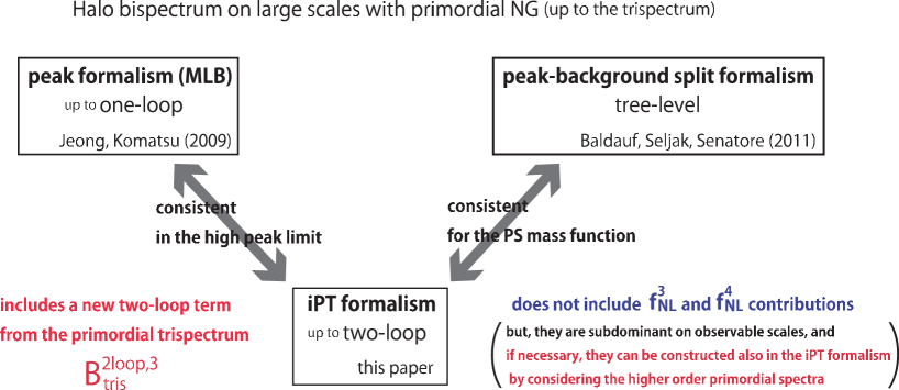
Figure 16: Summary of the consistency between three analytic formalism for the halo bispectrum with the primordial non-Gaussianity.

VI Summary

In this paper, on the basis of the iPT formalism, we have systematically investigated the bispectrum of the biased objects induced by the primordial non-Gaussianity. Basically, our formulae in the case of local-type non-Gaussianity are consistent with those of the previous works. Notable point in the present paper is that we studied the halo bispectrum in the case of not only the local-type, but also the equilateral- and orthogonal-type primordial non-Gaussianity. Further, in case of the local-type, we include the effect of the primordial trispectrum characterized by the two non-linearity parameters, $g_{\rm NL}$ and $\tau_{\rm NL}$. For the local-type non-Gaussianity, the two-loop correction coming from the terms proportional to $\tau_{\rm NL}$, denoted by $B_{\rm tris}^{2{\rm loop},3}$, is found to produce a non-negligible contribution, whose amplitude can become comparable to the dominant one-loop corrections proportional to $f_{\rm NL}^{2}$, denoted by $B_{\tau_{\rm NL}}$. As discussed in the previous section, such non-negligible loop contributions are represented by un-decomposable loop diagrams in the context of iPT, and taking account of such un-decomposable diagrams is rather crucial to precisely investigate the dominant contributions from the primordial non-Gaussianity. We stress here that the diagrammatic approach based on the iPT helps us to systematically collect these dominant contributions. The significance of higher-order contributions in the case of local-type non-Gaussianity is our important findings, and it implies that a much more great impact on the convergence of perturbative expansion is expected in the presence of higher-order primordial polyspectra. This should deserve further investigation, and we need a more clear and physical understanding of our results.

For the current observational upper-bound of the non-linearity parameters, the contributions from the primordial trispectrum would dominate the halo bispectrum on large scales. Taking the typical redshift and the mass of halos in surveys to be $z=1.0$ and $M=5\times 10^{13}h^{-1}M_{\odot}$ respectively, the halo bispectrum with $g_{\rm NL}=10^{4}$ is comparable to the one induced by $\tau_{\rm NL}=36f_{\rm NL}^{2}/25$ with $f_{\rm NL}=10$. In Ref. Sefusatti:2007ih , the authors mentioned that the future galaxy surveys would have a potential to detect $f_{\rm NL}\sim O(10)$, and this is expected to give $g_{\rm NL}<O(10^{4})$. The current observational limit on $g_{\rm NL}$ is about $g_{\rm NL}<O(10^{5})$ and hence the bispectrum of the biased object would be a powerful tool to obtain tighter constraint on $g_{\rm NL}$. For future idealistic wide-field surveys at $z=1$, in which we have a survey volume of $V=10h^{-3}{\rm Gpc}^{3}$ and the observable number density of the halos is $\bar{n}=10^{-4}h^{3}{\rm Mpc}^{-3}$ with typical mass $M=5\times 10^{13}h^{-1}M_{\odot}$, we expect that the detectability is improved to $g_{\rm NL}=O(10^{4})$. It is therefore very interesting to pursue a precise forecast for $g_{\rm NL}$ from the halo/galaxy bispectrum data obtained by the future surveys.

For equilateral- and orthogonal-types of non-Gaussianity, we find that the one-loop corrections are all suppressed and the tree-level calculation is sufficient to investigate the dominant contribution of halo bispectrum. Following the result obtained by Ref. Sefusatti:2007ih , future galaxy surveys can have a potential to obtain a constraint on $f_{\rm NL}^{\rm equil}$ down to $f_{\rm NL}^{\rm equil}<O(50)$, and it is comparable to the constraint obtained from the CMB observations. We expect that such future surveys also give a tight constraint on $f_{\rm NL}^{\rm orth}$. In this paper, we did not consider the contribution from the trispectrum in the cases of equilateral- and orthogonal-types non-Gaussianity, because their scale dependence is strongly dependent of the model generating the primordial non-Gaussianity. Also, the exact form of primordial trispectrum is much more complicated compared to that of the local-type non-Gaussianity. We leave the discussion on the contribution from the equilateral or orthogonal trispectrum to future work. Finally, while the recent cosmological $N$-body simulations suggest that the measured halo bispectrum on large scales is consistent with the previous analytic formulae Ref. Nishimichi:2009fs ; Sefusatti:2011gt ; Baldauf:2010vn , we believe that our formalism is capable of giving much more precise prediction which quantitatively reproduces the simulation results for various types of the primordial non-Gaussianity even on smaller scales. Along the line of this, the detailed comparison with $N$-body simulation is our important next subject.

Appendix A The choice of the mass function

Throughout this paper, we apply the Sheth-Tormen fitting formula as a mass function in the derivation of the scale-independent bias parameter $b_{n}^{\rm L}$. Let us discuss the dependence of the halo bispectrum on the choice of the mass function. For the Press-Schechter (PS) mass function given by

$$f_{\rm MF}(\nu)=f_{\rm PS}(\nu)=\sqrt{2\over\pi}\nu e^{-\nu^{2}/2},$$ (146)

we have the Lagrangian bias parameter as

$$b_{1}^{\rm L}={\nu^{2}-1\over\delta_{c}},~{}b_{2}^{\rm L}={\nu^{4}-3\nu^{2}\over\delta_{c}^{2}},~{}\cdots.$$ (147)

For the high peak formalism (HP) corresponding the large $\nu=\delta_{c}/\sigma_{M}$ limit, we have

$$b_{1}^{\rm L}={\nu^{2}\over\delta_{c}},~{}b_{2}^{\rm L}={\nu^{4}\over\delta_{c}^{2}},~{}b_{3}^{\rm L}={\nu^{6}\over\delta_{c}^{3}},\cdots$$ (148)

The Sheth-Tormen fitting formula (ST) is given by

$$f_{\rm MF}(\nu)=f_{\rm ST}(\nu)=A(p)\sqrt{{2\over\pi}}\left[1+(q\nu^{2})^{-p}\right]\sqrt{q}\nu e^{-q\nu^{2}/2},$$ (149)

and the MICE mass function (MICE) Crocce:2009mg is given by

$$f_{\rm MF}(\nu)=f_{\rm MICE}(\nu)=A_{\rm MICE}\left[\left({\nu\over\delta_{c}}\right)^{a}+b\right]e^{-c\nu^{2}/\delta_{c}^{2}},$$ (150)

with $A_{\rm MICE}(z)=0.58(1+z)^{-0.13}$, $a(z)=1.37(1+z)^{-0.15}$, $b(z)=0.3(1+z)^{-0.084}$, and $c(z)=1.036(1+z)^{-0.024}$. In Fig. 17,

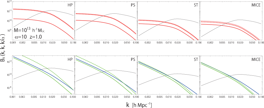
Figure 17: Each contribution of the halo bispectrum, Top - $B_{\rm grav}$ (black), $B_{\rm bis}^{\rm tree}$ (red thick), $B_{\rm bis}^{{\rm loop},1}$ (red thick dashed), and $B_{\rm bis}^{{\rm loop},2}$ (red thick dotted), Bottom - $B_{\rm grav}$ (black), $B_{g_{\rm NL}}$ (blue thick), $B_{\tau_{\rm NL}}$ (green thick), and $B_{\rm tris}^{{\rm loop},3}$ (green thick dashed) with tthe scale-independent bias parameters given by Eq. (148) (HP), and the mass function given by (146) (PS), (149) (ST) and (150) (MICE) from left to right.

we plot each contribution of the halo bispectrum, $B_{\rm grav}$ (black), $B_{\rm bis}^{\rm tree}$ (red thick), $B_{\rm bis}^{{\rm loop},1}$ (red thick dashed), and $B_{\rm bis}^{{\rm loop},2}$ (red thick dotted) in top panels, and $B_{\rm grav}$ (black), $B_{g_{\rm NL}}$ (blue thick), $B_{\tau_{\rm NL}}$ (green thick), and $B_{\rm tris}^{{\rm loop},3}$ (green thick dashed) in bottom panels, with the scale-independent bias parameters given by Eq. (148) (HP), and the mass function given by (146) (PS), (149) (ST) and (150) (MICE) from left to right. For the halo with mass $M=5\times 10^{13}h^{-1}M_{\odot}$ at $z=1.0$, we have $\nu=2.68$. In this figure, we find that the amplitude of the halo bispectrum is also strongly dependent on the choice of the mass function.

References

- (1) P. A. R. Ade et al. [Planck Collaboration], arXiv:1303.5084 [astro-ph.CO].
- (2) A. Slosar, C. Hirata, U. Seljak, S. Ho and N. Padmanabhan, JCAP 0808, 031 (2008) [arXiv:0805.3580 [astro-ph]].
- (3) T. Giannantonio, A. J. Ross, W. J. Percival, R. Crittenden, D. Bacher, M. Kilbinger, R. Nichol and J. Weller, arXiv:1303.1349 [astro-ph.CO].
- (4) N. Dalal, O. Dore, D. Huterer and A. Shirokov, Phys. Rev. D 77, 123514 (2008) [arXiv:0710.4560 [astro-ph]].
- (5) S. Matarrese and L. Verde, Astrophys. J. 677, L77 (2008) [arXiv:0801.4826 [astro-ph]].
- (6) D. Jeong and E. Komatsu, Astrophys. J. 703, 1230 (2009) [arXiv:0904.0497 [astro-ph.CO]].
- (7) E. Sefusatti and E. Komatsu, Phys. Rev. D 76 (2007) 083004 [arXiv:0705.0343 [astro-ph]].
- (8) E. Sefusatti, Phys. Rev. D 80, 123002 (2009) [arXiv:0905.0717 [astro-ph.CO]].
- (9) T. Baldauf, U. Seljak and L. Senatore, JCAP 1104, 006 (2011) [arXiv:1011.1513 [astro-ph.CO]].
- (10) T. Nishimichi, A. Taruya, K. Koyama and C. Sabiu, JCAP 1007, 002 (2010) [arXiv:0911.4768 [astro-ph.CO]].
- (11) T. Abbott et al. [Dark Energy Survey Collaboration], astro-ph/0510346.
- (12) D. Schlegel et al. [BigBoss Experiment Collaboration], arXiv:1106.1706 [astro-ph.IM].
- (13) P. A. Abell et al. [LSST Science and LSST Project Collaborations], arXiv:0912.0201 [astro-ph.IM].
- (14) R. Laureijs et al. [EUCLID Collaboration], arXiv:1110.3193 [astro-ph.CO].
- (15) R. Ellis et al. [PFS Team Collaboration], arXiv:1206.0737 [astro-ph.CO].
- (16) T. Matsubara, Phys. Rev. D 83, 083518 (2011) [arXiv:1102.4619 [astro-ph.CO]].
- (17) T. Matsubara, Phys. Rev. D 86, 063518 (2012) [arXiv:1206.0562 [astro-ph.CO]].
- (18) S. Yokoyama and T. Matsubara, Phys. Rev. D 87, 023525 (2013) [arXiv:1210.2495 [astro-ph.CO]].
- (19) M. Sato and T. Matsubara, arXiv:1304.4228 [astro-ph.CO].
- (20) G. Hinshaw et al. [WMAP Collaboration], Astrophys. J. Suppl. 208, 19 (2013) [arXiv:1212.5226 [astro-ph.CO]].
- (21) F. Bernardeau, M. Crocce and R. Scoccimarro, Phys. Rev. D 78, 103521 (2008) [arXiv:0806.2334 [astro-ph]].
- (22) T. Matsubara, arXiv:1304.4226 [astro-ph.CO].
- (23) T. Suyama and M. Yamaguchi, Phys. Rev. D 77, 023505 (2008) [arXiv:0709.2545 [astro-ph]].
- (24) T. Suyama, T. Takahashi, M. Yamaguchi and S. Yokoyama, JCAP 1012, 030 (2010) [arXiv:1009.1979 [astro-ph.CO]].
- (25) N. S. Sugiyama, E. Komatsu and T. Futamase, Phys. Rev. Lett. 106, 251301 (2011) [arXiv:1101.3636 [gr-qc]].
- (26) J. Bramante and J. Kumar, JCAP 1109, 036 (2011) [arXiv:1107.5362 [astro-ph.CO]].
- (27) N. S. Sugiyama, JCAP 1205, 032 (2012) [arXiv:1201.4048 [gr-qc]].
- (28) D. Tseliakhovich, C. Hirata and A. Slosar, Phys. Rev. D 82, 043531 (2010) [arXiv:1004.3302 [astro-ph.CO]].
- (29) K. M. Smith and M. LoVerde, JCAP 1111, 009 (2011) [arXiv:1010.0055 [astro-ph.CO]].
- (30) J. -O. Gong and S. Yokoyama, arXiv:1106.4404 [astro-ph.CO].
- (31) T. Nishimichi, JCAP 1208, 037 (2012) [arXiv:1204.3490 [astro-ph.CO]].
- (32) M. Biagetti, V. Desjacques and A. Riotto, arXiv:1208.1616 [astro-ph.CO].
- (33) D. Baumann, S. Ferraro, D. Green and K. M. Smith, JCAP 1305, 001 (2013) [arXiv:1209.2173 [astro-ph.CO]].
- (34) R. K. Sheth and G. Tormen, Mon. Not. Roy. Astron. Soc. 308, 119 (1999) [astro-ph/9901122].
- (35) S. Mizuno and K. Koyama, JCAP 1010, 002 (2010) [arXiv:1007.1462 [hep-th]].
- (36) K. Izumi, S. Mizuno and K. Koyama, Phys. Rev. D 85, 023521 (2012) [arXiv:1109.3746 [astro-ph.CO]].
- (37) E. Sefusatti, M. Crocce and V. Desjacques, arXiv:1111.6966 [astro-ph.CO].
- (38) M. Crocce, P. Fosalba, F. J. Castander and E. Gaztanaga, Mon. Not. Roy. Astron. Soc. 403, 1353 (2010) [arXiv:0907.0019 [astro-ph.CO]].
- (39) S. Matarrese, F. Lucchin and S. A. Bonometto, Astrophys. J. 310, L21 (1986).