Red giants seismology

Abstract

The space-borne missions CoRoT and Kepler are indiscreet. With their asteroseismic programs, they tell us what is hidden deep inside the stars. Waves excited just below the stellar surface travel throughout the stellar interior and unveil many secrets: how old is the star, how big, how massive, how fast (or slow) its core is dancing. This paper intends to paparazze the red giants according to the seismic pictures we have from their interiors.

1 Introduction

As denoted by many authors, red giant seismology is an exquisite surprise provided by the space missions CoRoT and Kepler. The analysis of a wealth of light curves recorded with unique length, continuity and photometric precision has already revealed many secrets. The most striking results, up to now, are provided by the observation of mixed modes (Fig. 1). Such modes result from the coupling of gravity waves, propagating in the radiative core region, with pressure waves propagating in the stellar envelope. They directly reveal information from the stellar core: the nature of the nuclear reaction (Bedding et al. 2011) and the mean core rotation rate (Beck et al. 2012).

An analysis of red giant seismic observational results has been given in Mosser (2013). Tricky points related to the data analysis are presented in a companion paper (Mosser et al. 2013a), where emphasis is given on red giant interior structure as revealed by asteroseismology. Only ensemble asteroseismology results are presented in this paper, obtained from the monitoring of a cohort of stars. Analysis and modelling of individual stars are not considered. They have started for a handful of targets (di Mauro et al. 2011; Jiang et al. 2011; Baudin et al. 2012). Such individual analysis are crucial for enhancing the understanding of the stellar interior structure and of the physical input to be considered, such as the measurement of the location of the helium second-ionization region (Miglio et al. 2010), or the measurement of differential rotation (Beck et al. 2012; Deheuvels et al. 2012).

In this work, ensemble asteroseismology results are derived from the observations of evolutionary sequences (Section 2). For red giants, asteroseismology benefits from the large homology of their interior structure, which translates into homologous properties of the oscillation spectrum (Section 3). In this Section, we also show how mixed-modes directly probe the stellar cores, and then investigate how stellar evolution is monitored by seismology on the RGB and in the red clump. Scaling relations derived from the homologous properties of red giants are discussed in Section 4, with a special emphasis on the mass and radius scaling relations and on their calibration. Rotation is discussed in Section 5. A recent leap toward oscillations detected in semi-regular variables is presented in Section 6.

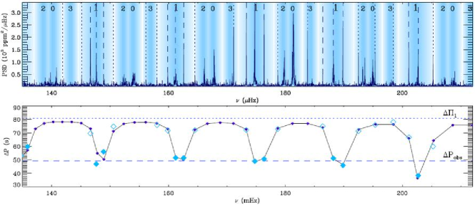
Figure 1: Top: Typical red giant oscillation pattern. Radial ($\ell=0$) and quadrupole ($\ell=2$) follow a regular comb pattern. Bottom: Period spacing between dipole modes; they have a mixed character and therefore show an irregular pattern; they can be identified with the asymptotic expansion. Figure from Mosser et al. (2012c).

2 Evolutionary sequences

The observation of thousands of red giants with CoRoT (e.g., Dupret et al. 2009; Mosser et al. 2010) and Kepler (e.g., Huber et al. 2010; Stello et al. 2013) allows us to address ensemble asteroseismology. According to the distance measurements derived from the scaling relations, red giants with magnitudes up to 13 are monitored vast regions of the Galaxy (Section 4.5). They show a large variety of metallicity (Bruntt et al. 2012). Independent of a specific population analysis (e.g., Silva Aguirre et al. 2011, for a one-solar-mass evolutionary sequence), we note that, apparently, the cohort of stars provided by both missions provide evolution sequence of low-mass stars. A reason justifying that we address sequences of evolution is provided by the global asteroseismic parameters $\nu_{\mathrm{max}}$ and $\Delta\nu_{\mathrm{obs}}$: $\nu_{\mathrm{max}}$ is the frequency of maximum oscillation signal; $\Delta\nu_{\mathrm{obs}}$ is the mean large frequency separation of radial modes observed around $\nu_{\mathrm{max}}$ (e.g., Mosser & Appourchaux 2009). The frequency $\nu_{\mathrm{max}}$ provides a proxy of the acoustic cutoff frequency, hence of $M\ R^{-2}\,{T_{\mathrm{eff}}}^{-1/2}$ (Belkacem et al. 2011). Following Belkacem et al. (2013), we consider that $\Delta\nu_{\mathrm{obs}}$ provides an acceptable proxy of the dynamical frequency $\nu_{0}$ that scales as $\sqrt{\mathcal{G}M/R^{3}}$. From these scalings, we derive

$$\Delta\nu_{\mathrm{obs}}\simeq\nu_{0}\propto M^{-1/4}\ {T_{\mathrm{eff}}}^{3/8}\ \nu_{\mathrm{max}}^{3/4}.$$ (1)

On the main sequence, the frequency $\Delta\nu_{\mathrm{obs}}$ scales as $\nu_{\mathrm{max}}^{0.8}$ (Verner et al. 2011b). The discrepancy between this exponent and the 3/4 value in Eq. 1 is due to the fact that low-mass and high-mass evolution tracks are in different regions of the main sequence. On the contrary, the observed scaling exponent on the RGB is much closer to 3/4 (Fig. 2) since the RGB regroups the evolution of low-mass stars. The agreement between Eq. 1 and global oscillation parameters observed over more than four decades in the red giant regime, completed by measurements on red supergiant stars (Kiss et al. 2006), indicates that the stellar red giant populations observed by CoRoT or Kepler constitute a set of stars homogenous enough to mimic stellar evolution, then justifying the relevance of the scaling relations. The difference between the observed exponent and 3/4 is small enough to be interpreted either by the very low variation of ${T_{\mathrm{eff}}}$ with $\nu_{\mathrm{max}}$, or by the difference between $\Delta\nu_{\mathrm{obs}}$ and $\nu_{0}$, and by other parameters that need to be calibrated but necessary have a limited influence. Masses in the range $0.9$ – $2\,M_{\odot}$ are present at all stages, hence for all $\nu_{\mathrm{max}}$, so that the mass parameter in Eq. 1 plays no significant role.

Before addressing the scaling relations, we discuss about stellar homology, seen by both radial and non-radial oscillation modes.

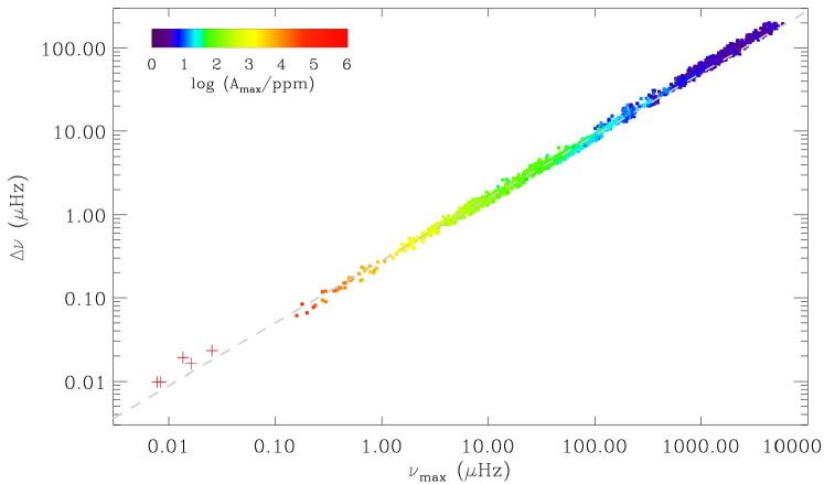
Figure 2: $\nu_{\mathrm{max}}$ – $\Delta\nu_{\mathrm{obs}}$ relation, with data from Verner et al. (2011b), Mosser et al. (2012c), and Mosser et al. (2013b). Plusses are red supergiants showing at least two oscillation modes observed by Kiss et al. (2006), with $\Delta\nu_{\mathrm{obs}}$ and $\nu_{\mathrm{max}}$ derived from a combination of the frequencies. The colors code the mean maximum amplitude $A_{\mathrm{max}}$ of the radial oscillations. The grey dashed line has a slope 3/4, in agreement with Eq. 1

3 Homology

3.1 From interior structure homology to seismic homology

Red giant interior structure is divided in three main regions; the dense helium core, the surrounding thin hydrogen-burning shell, and the thick, mostly convective envelope (Kippenhahn & Weigert 1990). Homology is ensured by the fact that this structure is dominated by generic physics: the thermodynamical conditions of the hydrogen-burning shell being related on the one side with the helium core and on the other side with the convective envelope, the core and envelope properties are closely linked together (Montalbán et al. 2013). Consequently, CoRoT observations have shown evidence of a very simple and useful property of the red giant oscillation pattern: following the interior structure homology, the oscillation pattern can also be defined as homologous. The concept of universal red giant oscillation pattern was therefore introduced by Mosser et al. (2011b), as an alternative form to the usual asymptotic expansion (Tassoul 1980), with the observed large separation as the only free parameter. The second-order asymptotic expansion expresses, for low angular degrees ($\ell\ll n$), as

$$\nu_{n,\ell}=\left(n+\varepsilon_{\mathrm{obs}}(\Delta\nu_{\mathrm{obs}})+d_{0\ell}(\Delta\nu_{\mathrm{obs}})+{\alpha\over 2}\,(n-n_{\mathrm{max}})^{2}\right)\ \Delta\nu_{\mathrm{obs}},$$ (2)

where the dimensionless parameter $n_{\mathrm{max}}$ is defined by $\nu_{\mathrm{max}}/\Delta\nu_{\mathrm{obs}}-\varepsilon_{\mathrm{obs}}$. Homology is expressed by the dependence in the observed large separation $\Delta\nu_{\mathrm{obs}}$ of the offsets $\varepsilon_{\mathrm{obs}}$ and $d_{0\ell}$. The radial offset $\varepsilon_{\mathrm{obs}}$ helps locate the radial ridge; the non-radial offsets $d_{0\ell}$ express the shifts of the different degrees $\ell$ compared to the radial modes (e.g., Corsaro et al. 2012). Homology is illustrated in Fig. 3, where Kepler red giant oscillation spectra are plotted on the same graph, with a dimensionless frequency in abscissa, and sorted by increasing large separation values. The alignment of the ridges, each one corresponding to a given radial order $n$ and angular degree $\ell$, demonstrates the universality of the oscillation pattern.

The form of Eq. 2, which includes a quadratic term, accounts for the measurement of $\Delta\nu_{\mathrm{obs}}$ around $\nu_{\mathrm{max}}$ in non-asymptotic conditions. The asymptotic form writes

$$\nu_{n,\ell}=\left(n^{\prime}_{\ell}+{A_{\ell}\over n^{\prime}_{\ell}}\right)\ \Delta\nu_{\mathrm{as}}\hbox{ \ with \ }n^{\prime}_{\ell}=n+\varepsilon_{\mathrm{as}}+{\ell\over 2}$$ (3)

The asymptotic large separation $\Delta\nu_{\mathrm{as}}$ is slightly greater than the observed value. The link between the observed and asymptotic parameters is explored in Mosser et al. (2013c). The asymptotic counterpart of $\varepsilon_{\mathrm{obs}}$ is, for low-mass stars, $\varepsilon_{\mathrm{as}}\equiv 1/4$ (Tassoul 1980). The high accuracy level reached by Eq. 2 has been show in previous comparison work (Verner et al. 2011b; Hekker et al. 2011, 2012). A quantitative analysis of the accuracy of the measurement of $\Delta\nu_{\mathrm{obs}}$ with Eq. 2 is done in Mosser et al. (2013a): the uncertainty is about $0.02\,\mu$Hz for all evolutionary stages.

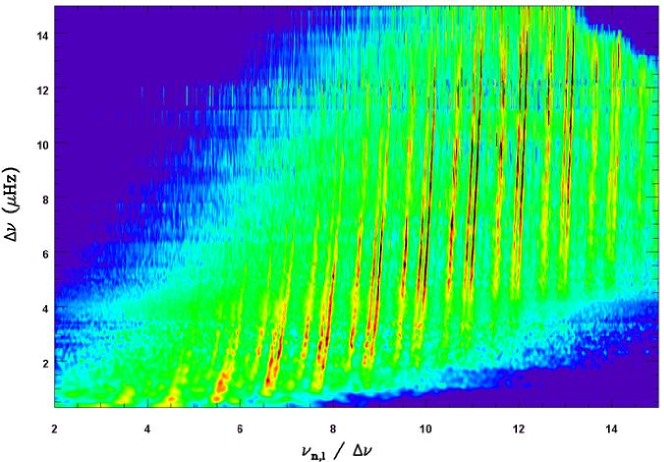
Figure 3: Kepler red giant oscillation spectra, as a function of the dimensionless frequency $\nu_{n,\ell}/\Delta\nu$, sorted by increasing large separation (y-axis). The colors code the oscillation amplitude normalized to the maximum oscillation signal. The close parallel ridges are drawn by quadrupole and radial modes, from the radial orders 3 to 13; the width of the dipole ridges is wider, due to the presence of mixed modes.

3.2 Sounding the core

Asteroseismology aims at probing the whole stellar interior structure. In the Sun, such an analysis performs very efficiently, but less efficiently in the core, since pressure modes do not probe the core as efficiently as they probe the other regions, the number of pressure modes sounding the solar core being low. This explains the quest for solar gravity modes that precisely probe the core (Appourchaux et al. 2010).

In red giants, g modes are not present, but appear indirectly through the coupling of gravity waves propagating in the core with pressure waves propagating in the envelope. A toy model for explaining this coupling is given in Mosser et al. (2013a). Since the first observation of mixed modes in red giants (Beck et al. 2011), a wealth of information has been provided by their analysis. Bedding et al. (2011) and Mosser et al. (2011a) have shown that different mixed-mode patterns help distinguish helium-core burning giants in the red clump from hydrogen-shell burning giants on the RGB. Mosser et al. (2012c) have proposed that an asymptotic expansion is able to depict the mixed-mode pattern. This expansion, derived from the formalism developed by Unno et al. (1989), introduces the gravity period spacing $\Delta\Pi_{1}$ defined by an integral function of the Brunt-Väisälä frequency in the inner radiative region. The measured values of $\Delta\Pi_{1}$ are accurately reproduced for red giant ascending the RGB, but not in the clump (Montalbán et al. 2013). This discrepancy in the clump is not yet understood and deserves further work.

Homology seen in the radial red giant oscillation pattern is also seen in the $\Delta\nu$ – $\Delta\Pi_{1}$ diagram (Fig. 4). All low-mass stars on the RGB lie on the same track, independent of their mass and composition. With $\Delta\nu$ representing the stellar mean density and $\Delta\Pi_{1}$ representing the density of the core, we derive from Fig. 4 that the properties of the core and of the envelope are closely correlated. The inert helium core of an RGB star necessarily contracts when the star ascends the RGB; accordingly, its mass increases, as a result of the hydrogen burning shell which surrounds it. Its contraction and mass increase yield a decreasing $\Delta\Pi_{1}$ term, as observed and as seen in the modeling (Montalbán et al. 2013). This contraction implies that the density of the hydrogen burning shell increases. This increase boosts the energy production. Hence, the hydrogen envelope expands.

Homology is reinforced in the red clump, since a further similar event has participated to erase the initial differences between low-mass stars. Their helium core being degenerate, the helium flash occurs in very similar conditions (Montalbán et al. 2013), so that they nearly reach the same location in the $\Delta\Pi_{1}$ – $\Delta\nu_{\mathrm{obs}}$ diagram, close to $\Delta\Pi_{1}\simeq 300\,$s and $\Delta\nu\simeq 4\,\mu$Hz.

The precision we have on the mixed mode determination is so high that we may expect, from an accurate modelling, a highly precise age determination. During the evolution on the RGB, the gravity period spacing $\Delta\Pi_{1}$ change is about 100 s (Fig. 4). Since the measurement of $\Delta\Pi_{1}$ is more precise than 0.1 s, it is formally possible to track the timing of the ascent of a red giant with a precision as high as 0.1 %.

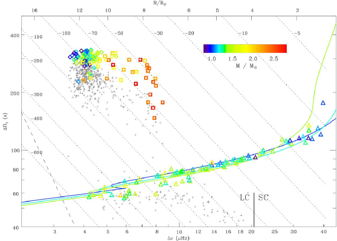
Figure 4: Gravity-mode period spacing $\Delta\Pi_{1}$ as a function of the pressure-mode large frequency spacing $\Delta\nu$, for a set of red giants observed with Kepler. Long-cadence data (LC) have $\Delta\nu\leq 20.4\,\mu$Hz. RGB stars are indicated by triangles; clump stars by diamonds; secondary clump stars by squares. Uncertainties in both parameters are smaller than the symbol size. The seismic estimate of the mass is given by the color code. Small gray crosses indicate the bumped periods $\Delta P$ measured by Mosser et al. (2011a). Dotted lines are $n_{\mathrm{g}}$ isolines. The dashed line in the lower left corner indicates the formal frequency resolution limit. The upper x-axis gives an estimate of the stellar radius for a star whose $\nu_{\mathrm{max}}$ is related to $\Delta\nu$ according to the mean scaling relation $\nu_{\mathrm{max}}=(\Delta\nu/0.28)^{1.33}$ (both frequencies in $\mu$Hz). The solid colored lines correspond to a grid of stellar models with masses of 1, 1.2 and $1.4\,M_{\odot}$, from the ZAMS to the tip of the RGB. Figure from Mosser et al. (2012c).

Table 1: Scaling relations

parameter		unit	coefficient $\alpha$	exponent $\beta$
large separation	$\Delta\nu_{\mathrm{obs}}$	$\mu$Hz	$0.274\pm 0.004$	$0.757\pm 0.004$
	$n_{\mathrm{max}}=\nu_{\mathrm{max}}/\Delta\nu-\varepsilon_{\mathrm{obs}}$	–	$3.26\pm 0.031$	$0.242\pm 0.005$
FWHM	$\delta\nu_{\mathrm{env}}$	$\mu$Hz	$0.73\pm 0.03$	$0.88\pm 0.01$
	$n_{\mathrm{env}}=\delta\nu_{\mathrm{env}}/\Delta\nu$	–	$2.49\pm 0.12$	$0.13\pm 0.01$
Height at $\nu_{\mathrm{max}}$	$H_{\mathrm{max}}$	ppm2 $\mu$Hz-1	$(2.03\pm 0.05)\;10^{7}$	$-2.38\pm 0.01$
Background at $\nu_{\mathrm{max}}$	$B_{\mathrm{max}}$	ppm2 $\mu$Hz-1	$(6.37\pm 0.02)\;10^{6}$	$-2.41\pm 0.01$
HBR	$H_{\mathrm{max}}/B_{\mathrm{max}}$	–	$3.18\pm 0.09$	$0.03\pm 0.03$
Granulation	$P_{\mathrm{g}}$	ppm2 $\mu$Hz-1		$-2.15\pm 0.12$
	$\tau_{\mathrm{g}}$	s		$-0.90\pm 0.005$
	$P_{\mathrm{g}}(\tau_{\mathrm{g}})$	ppm2 $\mu$Hz-1		$2.34\pm 0.01$
radius	$R$	$R_{\odot}$	$63.1\pm 1.1$	$-0.49\pm 0.01$
effective temperature	${T_{\mathrm{eff}}}$	K	$3922\pm 50$	$0.051\pm 0.05$

- All results were obtained with the COR pipeline (Mosser et al. 2012a). Granulation data are from Mathur et al. (2011).

- Each parameter is estimated as a power law of $\nu_{\mathrm{max}}$, with $\alpha$ the coefficient and $\beta$ the exponent, except $P_{\mathrm{g}}(\tau_{\mathrm{g}})$.

4 Scaling relations

4.1 Seismic parameters

As a result of homology, the red giant global seismic parameters conform to a large numbers of scaling relations. Their variations with $\nu_{\mathrm{max}}$ are summarized in Table 1, where we consider:

- The mean observed large separation $\Delta\nu_{\mathrm{obs}}$ measured in a broad frequency range around $\nu_{\mathrm{max}}$, and $n_{\mathrm{max}}=\nu_{\mathrm{max}}/\Delta\nu_{\mathrm{obs}}-\varepsilon_{\mathrm{obs}}$ which provides an estimate of the radial order at $\nu_{\mathrm{max}}$; $n_{\mathrm{max}}$ significantly decreases when $\Delta\nu_{\mathrm{obs}}$ decreases. For the Sun, $n_{\mathrm{max}}\simeq 22$; at the red clump, $n_{\mathrm{max}}\simeq 8$; and at the tip of the RGB, $n_{\mathrm{max}}\simeq 2.5$.

- $\delta\nu_{\mathrm{env}}$ is the full-width at half-maximum of the smoothed excess power; $n_{\mathrm{env}}=\delta\nu_{\mathrm{env}}/\Delta\nu_{\mathrm{obs}}$ provides $\delta\nu_{\mathrm{env}}$ is large separation unit; as $n_{\mathrm{max}}$, $n_{\mathrm{env}}$ significantly decreases when $\Delta\nu_{\mathrm{obs}}$ decreases since $\delta\nu_{\mathrm{env}}$ approximately scales as $\nu_{\mathrm{max}}$.

- $H_{\mathrm{max}}$ (in ppm${}^{2}\,\mu$Hz^-1) is the mean height of the modes at $\nu_{\mathrm{max}}$, defined according to the description of smoothed excess power as a Gaussian envelope (e.g., Mosser et al. 2012a).

- $B_{\mathrm{max}}$ (in ppm${}^{2}\,\mu$Hz^-1) is the value of the stellar background $B$ at $\nu_{\mathrm{max}}$. The background is described by Harvey-like components (Michel et al. 2008). Each component is a modified Lorentzian of the form $b(\nu)=a/[1+(2\pi\,\nu\tau)^{\alpha}]$, where $\tau$ is the characteristic time scale. The exponent $\alpha$ is in the range 2 – 4 (Mathur et al. 2011). $H_{\mathrm{max}}/B_{\mathrm{max}}$ is representative of the height to background ratio (HBR) at $\nu_{\mathrm{max}}$. This ratio shows no significant variation all along the RGB.

- Properties of the granulation signal are also considered (Mathur et al. 2011): $P_{\mathrm{g}}$ is the height of the granulation component ; $\tau_{\mathrm{g}}$ is the time scale of this background component related to the granulation signal. We note that the exponent of the $P_{\mathrm{g}}(\tau_{\mathrm{g}})$ scaling relation is, in absolute value, very close to the exponent of the $B_{\mathrm{max}}(\nu_{\mathrm{max}})$ scaling relation. This means that the energy content in the granulation and in the oscillations are certainly linked.

- Finally, we provide estimates of the fundamental parameters $R$ and ${T_{\mathrm{eff}}}$.

Some of the scaling relations are illustrated in Fig. 5 that shows, compared to the Sun, oscillation spectra of red giants from the bottom to the top of the RGB. Currently, we lack theoretical models for explaining most of these relations. Large efforts have been devoted to explain the scaling relations of the mean amplitude $A_{\mathrm{max}}$. This global parameter can be fitted, in limited frequency range, as in Mosser et al. (2012a). However, the fit heavily depends on the method (Stello et al. 2011a; Huber et al. 2011), so that it is not yet possible to provide a physically relevant result (Corsaro et al. 2013). Samadi et al. (2012) have shown that scaling relations of mode amplitudes cannot be extended from main-sequence to red giant stars because non-adiabatic effects for red giant stars cannot be neglected. Samadi et al. (2013a) have recently proposed a theoretical model of the oscillation spectrum associated with the stellar granulation as seen in disk-integrated intensity. With this model, Samadi et al. (2013b) have highlighted the role of the photospheric Mach number for controlling the properties of the stellar granulation.

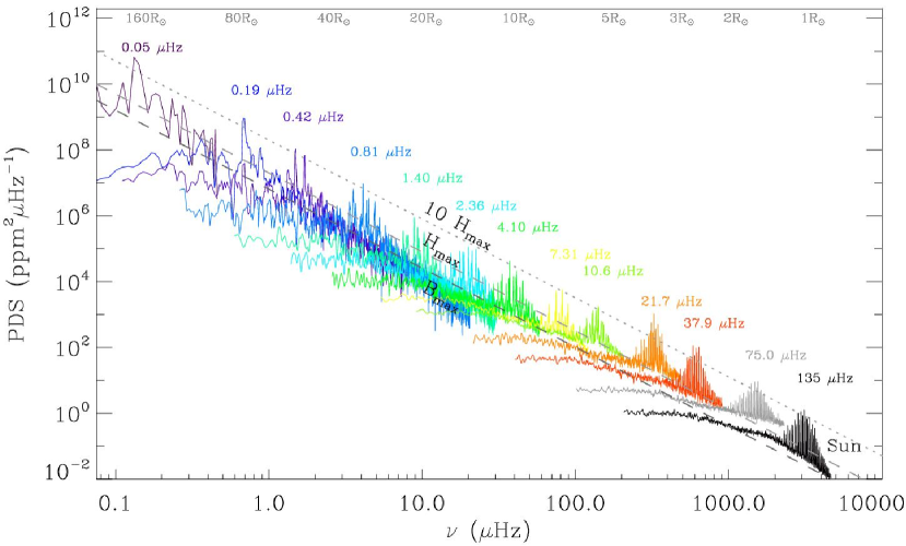
Figure 5: Superimposition of red giant oscillation spectra from the bottom to the tip of the RGB. Each spectrum is identified by the large separation $\Delta\nu_{\mathrm{obs}}$. The Sun spectrum (in black) and another main-sequence spectrum (in grey) are shown for comparison. Except at very low frequency, all spectra were filtered, with a filter width varying with $\nu_{\mathrm{max}}$. The fit of the background and mean height at $\nu_{\mathrm{max}}$ (Table 1) are indicated with dashed lines. A proxy of the stellar radius is provided along the upper frequency ($\nu_{\mathrm{max}}$) axis. Data from Mosser et al. (2012c) and Mosser et al. (2013b)

4.2 Mass and radius scaling relations

As already stated, the seismic global parameters $\nu_{\mathrm{max}}$ and $\Delta\nu$ scale, respectively, as the atmospheric cutoff frequency and as the square root of the mean density. Hence, seismic relations with $\Delta\nu_{\mathrm{obs}}$ and $\nu_{\mathrm{max}}$ can be used to provides proxies of the stellar masses and radii. Following Mosser et al. (2013c), we stress that it is necessary to avoid confusion between the large separation $\Delta\nu_{\mathrm{obs}}$ observed around $\nu_{\mathrm{max}}$, the asymptotic large separation $\Delta\nu_{\mathrm{as}}$, and the dynamical frequency $\nu_{0}$ that scales with $\sqrt{\mathcal{G}M/R^{3}}$. The measurement of $\Delta\nu_{\mathrm{obs}}$ is perturbed by frequency glitches due to the rapid local variation of the sound speed in the stellar interior, related to the density contrast at the core boundary or to the local depression of the sound speed that occurs in the helium second-ionization region (Miglio et al. 2010). The scaling relations write then:

$${R\over R_{\odot}}=\left({\nu_{\mathrm{max}}\over\nu_{\mathrm{ref}}}\right)\ \left({\Delta\nu_{\mathrm{as}}\over\Delta\nu_{\mathrm{ref}}}\right)^{-2}\left({{T_{\mathrm{eff}}}\over T_{\odot}}\right)^{1/2},$$ (4)

$${M\over M_{\odot}}=\left({\nu_{\mathrm{max}}\over\nu_{\mathrm{ref}}}\right)^{3}\left({\Delta\nu_{\mathrm{as}}\over\Delta\nu_{\mathrm{ref}}}\right)^{-4}\left({{T_{\mathrm{eff}}}\over T_{\odot}}\right)^{3/2},$$ (5)

with the calibrated references $\nu_{\mathrm{ref}}=3104\,\mu$Hz and $\Delta\nu_{\mathrm{ref}}=138.8\,\mu$Hz. Such reference values were determined in order to avoid systematic bias between the seismic proxies and modeled values (Mosser et al. 2013c).

Compared to scaling relations heavily used elsewhere (e.g., Mosser et al. 2010; Kallinger et al. 2010; Chaplin et al. 2011; Verner et al. 2011a; Silva Aguirre et al. 2011; Stello et al. 2013; Hekker et al. 2013), Eqs. 4 and 5 make use of the asymptotic large separation instead of the observed large separation. They introduce a correction which can be expressed by

$$R_{\mathrm{as}}\simeq\bigl{[}{1-2\,(\zeta-\zeta_{\odot})}\bigr{]}R_{\mathrm{obs}}\hbox{ \ and \ }M_{\mathrm{as}}\simeq\bigl{[}{1-4\,(\zeta-\zeta_{\odot})}\bigr{]}M_{\mathrm{obs}},$$ (6)

with $\zeta=0.57/n_{\mathrm{max}}$ in the main-sequence regime and $\zeta=0.038$ in the red giant regime. The amplitude of the correction takes into account the fact that scaling relations are calibrated on the Sun, so that one has to deduce the solar correction $\zeta_{\odot}\simeq 0.026\,$%. These asymptotic corrections represent a first step towards the proper calibration of the relation. Contrary to the forms based on the observed large separation, they are not biased, and free of the perturbation of the glitches (Mosser et al. 2013a). This result might contradict Belkacem et al. (2013), who state that $\Delta\nu_{\mathrm{obs}}$ provides a better proxy of $\nu_{0}$ than $\Delta\nu_{\mathrm{as}}$. In fact, the contradiction is apparent only: the calibration effort has still to link the asymptotic values derived from the models or derived from the observations (Table 2).

Table 2: Calibration of the mass and radius scaling relations

	Modeling	Calibration	Observation
$M,R\leftrightarrow$	$\Delta\nu_{\mathrm{as,mod}}\leftrightarrow$	?	$\leftrightarrow\Delta\nu_{\mathrm{as,obs}}\leftrightarrow\Delta\nu_{\mathrm{obs}}$
	$\nu_{\mathrm{max,mod}}\leftrightarrow$	?	$\leftrightarrow\nu_{\mathrm{max,obs}}$

Calibration process unveiling all formal steps for a proper calibration of the mass and radius scaling relations, with checking of the asymptotic values, determined in the modeling process from $1/(2\int_{0}^{R}\mathrm{d}r/c)$ and in observations from the asymptotically corrected $\Delta\nu_{\mathrm{obs}}$.

4.3 Calibration of the mass and radius scaling relations

For a proper calibration of the mass and radius scaling relations, we should use the dynamical frequency $\nu_{0}$ instead of $\Delta\nu_{\mathrm{obs}}$ or $\Delta\nu_{\mathrm{as}}$, and the acoustic frequency $\nu_{\mathrm{c}}$ instead of $\nu_{\mathrm{max}}$. As this is not the case, an intensive calibration effort is undertaken:

- An independent verification has been made for stars that have accurate Hipparcos parallaxes, by coupling asteroseismic analysis with the InfraRed Flux Method (Silva Aguirre et al. 2012). The seismic distance determinations agree to better than 5 %: this shows the relevance and the accuracy of the scaling relations in the subgiant and main-sequence regime.

- With long-baseline interferometric measurement of the radius of five main-sequence stars, one subgiant and four red giant stars for which solar-like oscillations have been detected by either Kepler or CoRoT, Huber et al. (2012) have shown that scaling relations are in excellent agreement within the observational uncertainties. They finally derive that asteroseismic radii for main-sequence stars are accurate to better than 4 %.

- Oscillations in cluster stars (Basu et al. 2011) were used to compare scaling relations for red giants in the red clump or on the RGB. Miglio et al. (2012a) have found evidence for systematic differences in the $\Delta\nu_{\mathrm{obs}}$ scaling relation between He-burning and H-shell-burning giants. This implies that a relative correction between RGB and clump stars must be considered. As this correction is also related to mass loss, it is currently not possible to measure it precisely. Independent of this, oscillations in cluster stars provide useful constraints on membership (Stello et al. 2011b). They also help constrain the relations depicting the parameters of the pressure mode spectrum (Corsaro et al. 2012).

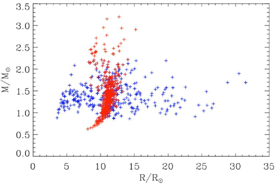
Figure 6: Mass – radius relation for Kepler red giants, with RGB stars in blue and clump stars in red. Adapted from Mosser et al. (2012a).

4.4 Radius, mass and mass loss

The mass and radius scaling relations are illustrated by a mass – radius diagram (Fig. 6). The uncertainties on the inferred mass and radius values discussed above warn us that the absolute values of the data reported here are not yet fully calibrated. However, the trends and the relative variations are relevant, so that it is possible to derive unique information:

- Most of the stellar masses observed on the RGB are in the range [1, $2\,M_{\odot}$]; less-massive stars spend a longer lifetime on the main sequence, so that they need time to reach the RGB; more massive stars are intrinsically rare and evolve quickly on different evolutionary tracks, especially in the instability strip. So, many of them do not experience solar-like oscillations before having met the RGB; they reach it with a larger radius than lower-mass stars;

- In the red clump, consequently after the tip of the RGB where strong episodes of mass loss occur, the mass distribution is significantly different. Stars with mass down to $0.6\,M_{\odot}$ are observed: they have necessarily suffered from efficient mass loss near the tip of the RGB. Stars with mass over $2\,M_{\odot}$ are present, since they spend more time in the helium-burning phase than ascending the RGB in the region where solar-like oscillations are observed.

- The mass-radius relation in the red clump shows a limited spread. All stars in this stage share common properties, as derived from the examination of the $\Delta\Pi_{1}$ – $\Delta\nu_{\mathrm{obs}}$ relation on the RGB (Fig. 4 and Section 3.2). If we add the information of the effective temperature in Fig. 6, we note that, at fixed mass, the hottest stars have the smallest radius, in agreement with a thinner envelope.

- Secondary-clump stars show a larger spread in the mass-radius diagram compared to clump stars. The difference may arise from the ignition of helium having started in non-degenerate conditions. As already stated above, the mass of transition between the primary and secondary clumps, about $1.8\,M_{\odot}$, is indicative only. Its precise determination requires the careful calibration of the scaling relation (Eq. 5).

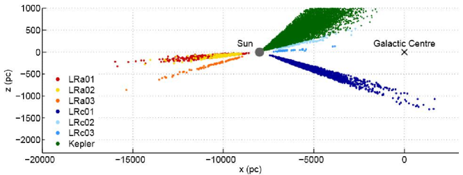
Figure 7: Solar-like oscillating red giants observed in several CoRoT fields of view and by Kepler: projection on the $x$ – $z$ plane. Figure from Miglio et al. (2012b).

4.5 Distance measurements and stellar population

An important consequence of the measurement of asteroseismic radii for field stars is the capability of measuring stellar distance. Miglio et al. (2013) have shown that red giants represent a well-populated class of accurate distance indicators, spanning a large age range, which can be used to map and date the Galactic disk in the regions probed by observations made by the CoRoT and Kepler. They have determined precise distances for 2000 stars spread across nearly 15 000 pc of the Galactic disk, exploring regions which are a long way from the solar neighbourhood (Fig. 7). Significant differences in the mass distributions of these two samples are interpreted as mainly due to the vertical gradient in the distribution of stellar masses (hence ages) in the disk.

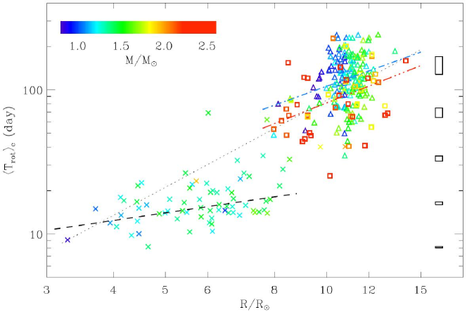
Figure 8: Mean period of core rotation as a function of the asteroseismic stellar radius, in log-log scale. The dotted line indicates a rotation period varying as $R^{2}$. The dashed (dot-dashed, triple-dot-dashed) line indicates the fit of RGB (clump, secondary clump) core rotation period. The rectangles in the right side indicate the typical error boxes, as a function of the rotation period. Figure from Mosser et al. (2012b).

5 Rotation

Rotational splittings have been first observed in a handful of red giants, putting in evidence a significant radial differential rotation (Beck et al. 2012; Deheuvels et al. 2012). Mosser et al. (2012c) have developed a dedicated method for automated measurements of the rotational splittings in a large number of red giants. They have also shown that these splittings, dominated by the core rotation, can be modeled with a Lorentzian function that resembles the mixed-mode pattern organization. Under the assumption that a linear analysis can provide the rotational splitting, they note a small decrease of the mean core rotation rate of stars ascending the RGB. Alternatively, an important slow down is observed for red-clump stars compared to the RGB. They also show that, at fixed stellar radius, the specific angular momentum increases with increasing stellar mass (Fig. 8).

With the same hypothesis of linear splittings, Goupil et al. (2013) have described the morphology of the rotational splittings. They have proven that the mean core rotation dominates the splittings, even for pressure dominated mixed modes. For red giant stars with slowly rotating cores, the variation in the rotational splittings of dipole modes with frequency depends only on the large frequency separation, the g-mode period spacing, and the ratio of the average envelope to core rotation rates. Thus, they have proposed a method to infer directly this ratio from the observations and have validated this method using Kepler data. In case of rapid rotation, rotation cannot be considered as a perturbation any more and the linear approach fails (Ouazzani et al. 2013).

For investigating the internal transport and surface loss of the angular momentum of oscillating solar-like stars, Marques et al. (2013) have studied the evolution of rotational splittings from the pre-main sequence to the red-giant branch (RGB) for stochastically excited oscillation modes. They have shown that transport by meridional circulation and shear turbulence cannot explain the observed spin-down of the mean core rotation. They suspect the horizontal turbulent viscosity to be largely underestimated.

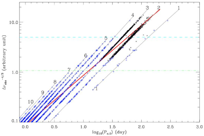
Figure 9: Period-luminosity relations with Kepler (blue) and OGLE data (black), from Mosser et al. (2013b). The blue dashed line indicates the location of the tip of the RGB.

6 Oscillations in evolved M giants

Semi-variability in evolved M giants is suspected to be due to solar-like oscillations. However, until recently, only indirect information was available for sustaining this hypothesis (e.g., Dziembowski & Soszyński 2010). The question concerning the nature of these oscillations is now solved with Kepler observations (Mosser et al. 2013b). According to scaling relations, such oscillations occur at very low frequency: at the tip of the RGB, $1/\nu_{\mathrm{max}}$ corresponds to periods of 50 days. The monitoring of such oscillations has benefitted from the unique length of Kepler observation (more than 3 years) and is unfortunately out of reach with CoRoT observations limited to five months (e.g., Barban et al. 2009).

The solution for unambiguously identifying solar-like oscillations at very low frequency is based on two arguments. First, the relevance of the universal red giant oscillation pattern for less-evolved evolutionary stages implies that, at late stages, oscillation spectra very certainly show homologous properties. Second, the $\varepsilon_{\mathrm{obs}}(\Delta\nu_{\mathrm{obs}})$ relation observed in the whole red giant oscillation regime is justified by the validity of the second-order asymptotic expansion. Consequently, this relation was extrapolated to very low $\nu_{\mathrm{max}}$, and iteratively adapted to provide an acceptable fit of the M-giant oscillation spectra. The success of the fits for all red giants, except in a limited number of cases with a very low signal-to-noise-ratio oscillation spectrum or frequency leakage due to binarity, has proven the relevance of the method.

Period-luminosity relations interpreted as solar-like oscillations are shown in Fig. 9; OGLE data are superimposed. When the large separation decreases, the radial orders of the observed modes decrease too, down to $n_{\mathrm{max}}=2$. The fits show that mostly radial $n=2$ and 3 modes are observed below the tip of the RGB. Interpreting oscillations in semi-regular variables has many consequences: the parametrization of the oscillation spectrum will help reanalyze the ground-based observations and to define more accurately the different sequences. Interpreting period-luminosity relations in red giants in terms of solar-like oscillations might by used to reinvestigate with a firm physical basis the time series obtained from ground-based microlensing surveys. This will provide improved distance measurements and open the way to extragalactic asteroseismology, with the observations of M giants in the Magellanic Clouds. Mosser et al. (2013b) have also shown that the acceleration of the external layers of red giant with solar-like oscillations is about the same order of magnitude as the surface gravity when the stars reach the tip of the RGB. This shows that oscillations might play a non-negligible role in the mass-loss process.

7 Conclusions?

Ensemble asteroseismology is an active field in current progress. Any conclusion written now will be out of date tomorrow. Plenty of work remains to be done:

- examining the fine structure of the universal red-giant oscillation pattern;

- establishing a thorough calibration of the mass and radius scaling relations;

- modelling a large number of stars, with improved stellar physics;

- deriving precise stellar ages;

- irrigating many connected themes: distance measurement, population study, gyrochronology, late stages evolution…

Following the successful space missions CoRoT and Kepler, a next-generation seismic project requires simple but demanding characteristics: long, continuous, and ultra-precise photometric observations. A complete survey of the sky, twin of the ESA Gaia mission, able to derive the seismic global indices $\Delta\nu_{\mathrm{obs}}$ and $\nu_{\mathrm{max}}$ for millions of stars, is certainly a highly-promising project.