Resonance mass spectra of gravity and fermion on Bloch branes

Abstract

In this paper, by presenting the potentials of Kaluza–Klein (KK) modes in the corresponding Schrödinger equations, we investigate the localization and resonances of gravity and fermion on the symmetric and asymmetric Bloch branes. We find that the localization properties of zero modes for gravity and fermion in the symmetric brane case are the same, whereas, for the asymmetric brane case, the fermion zero mode is localized on one of the sub-branes, while the gravity zero mode is localized on another sub-brane. The spectra of the gravity and the left- or right-handed fermion are composed of a bound zero mode and a series of gapless continuous massive KK modes. Among the continuous massive KK modes, we obtain some discrete gravity and fermion resonant (quasilocalized) KK states on the brane, which have a finite probability of escaping into the bulk. The KK states with lower resonant masses have a longer lifetime on the brane. And the number of the resonant KK states increases linearly with the width of the brane and the scalar-fermion coupling constant, but it decreases with the asymmetric factor $\beta$. The structure of the resonance spectrum is investigated in detail.

I Introduction

About ninety years ago, the idea of the possible existence of extra spatial dimensions was presented by Kaluza and Klein (KK) Kaluza1921 ; Klein1926 , who tried to unify four-dimensional (4D) Einstein gravity and electromagnetism by proposing a theory with a compact fifth dimension. However, the KK theory is not a viable model to describe nature because it has many problems. Later, in 1980s, our 4D universe was considered as a domain wall (topological defect) embedded in a higher-dimensional space-time Rubakov1983 ; Akama1983 ; Antoniadis1990 . After large ADD and warped rsI extra dimensions were respectively presented as a solution to the hierarchy problem, the idea of extra dimensions became popular. In this scenario, our 4D universe is an infinitely thin brane embedded in a higher dimensional space-time, and gravity is free to propagate in all dimensions, while all the Standard Model fields are localized on a 3-brane. In the Randall-Sundrum-1 (RS1) model rsI , there are two 3-branes located at the boundaries of a compact extra dimension with the topology $S^{1}/Z_{2}$, one with negative tension (the visible brane or TeV brane we lived on) and another with positive tension (the hidden brane or Planck brane). In this model, the gauge hierarchy problem is solved by an exponential warp factor $e^{-ky}$, but there is a modulus problem and we will get a “wrong-signed” Friedmann-like equation on our negative tension brane. Hence, in order to stabilize the modulus, one needs to introduce a scalar field in the bulk GW . In the RS2 model rsII , the extra dimension is infinite and there is only one brane with positive tension, on which gravity can be localized. The RS2 model does not suffer from the modulus problem and can reduce a right-signed Friedmann-like equation on the brane, but the hierarchy problem is left. Generalizations and extensions of the RS brane model can be found for examples in Refs. ExtensionRS ; littleStringBrane ; 1104.3188 ; scalar-tensor branes .

In this paper, we are interested in the generalization of the RS2 model, which is done by introducing background scalar fields in the bulk. In this generalization, bulk scalars play the role of generating the brane as a domain wall (thick brane). And a virtue is that branes can be realized naturally and have inner structure. Because of this, an increasing interest has been focused on investigation of thick branes generated by bulk scalar fields in higher dimensional space-time dewolfe ; GremmPLB2000 ; Csaki ; ThickBrane4 ; Liu0907.1952 ; George2010a ; George2010b ; Zhao2010 ; 1004.2181 ; Zhong2011 ; ThickBraneBazeia . For a review on thick brane solutions see Ref. ThickBraneReview .

Localization and spectra of various bulk fields including gravity on a brane is an important and interesting problem ThickBrane4 ; RandjbarPLB2000 ; Volkas2007 ; Liu0708 ; 20082009 ; Fu2011 ; Liu0803 ; LiLiu2011 ; Gogberashvili2012 ; Liu2012a ; Christiansen2012 . Because the effective physics in the low energy scale is four-dimensional, the lowest modes of various bulk fields should be localized on the brane in order not to contradict the current experiments. In order to localize fermions on branes, one needs to introduce localization mechanisms RandjbarPLB2000 . Usually the Yukawa coupling of fermions with background scalar fields Volkas2007 is introduced. Under this mechanism, there may exist a single bound massless fermion KK mode (i.e., the fermion zero mode) Liu0708 ; 20082009 ; Fu2011 , or a bound massless KK mode and finite discrete bound massive KK modes (mass gaps) ThickBrane4 ; Liu0803 . Furthermore, some other backgrounds, for example, supergravity Mario and gauge field Parameswaran0608074 could be also considered.

Fermions and gravity on symmetric double branes have been investigated in Refs. Guerrero2006 ; MelfoPRD2006 . There are two sub-branes located at the edges of the double brane. It was shown that the fermion zero mode on the double brane is not peaked at the center of the brane, but instead is a constant between the two sub-branes.

In Ref. BazeiaJHEP2004 , a kind of double brane, the so-called Bloch brane, was presented by Bazeia and Gomes. In this model, the system is described by two real scalar fields coupled with gravity in warped space-time. It was found that the parameter which controls the way the two scalar fields interact results in the appearance of a thick double brane with internal structure. In this paper, we would like to investigate the localization of fermion and gravity on the Bloch brane. Especially, we will find that there are many resonant KK modes for gravity and fermion on the double brane, which in fact are quasi localized KK modes. The resonant KK modes with lower resonant mass have a longer lifetime. We also construct an asymmetric Bloch brane and investigate localization of zero modes of gravity and fermion on it. It will be shown that the fermion zero mode is localized on one of the sub-branes, while the gravity zero mode is localized on another sub-brane. As far as we know, the resonant spectra of gravity and fermion on asymmetric branes still has not been investigated. Therefore, the resonant structure for gravity and fermion on the asymmetric Bloch brane will also be investigated in this paper.

The paper is organized as follows. In Sec. II, we first give a brief review of the symmetric Bloch brane in five-dimensional space-time, and construct asymmetric Bloch brane solutions. Then, in Sec. III, we study the zero mode and resonance mass spectrum of gravity on the symmetric and asymmetric thick brane by presenting the potential of the corresponding Schrödinger problem for the linear tensor perturbation KK modes of the metric. In Sec. IV, we investigate the localization and resonance mass spectrum of spin-half fermions on the symmetric and asymmetric thick brane with the typical scalar-fermion interaction. We simply compare the localization of the zero modes of gravity and fermion on the symmetric and asymmetric branes in Sec. V. Finally, a brief discussion and conclusion are presented in Sec. VI.

II Review of the model

Let us consider thick branes arising from two interacting real scalar fields $\phi$ and $\chi$ with a scalar potential $V(\phi,\chi)$. The action for such a system is given by

$$S=\int d^{5}x\sqrt{-g}\left[\frac{1}{4}R-\frac{1}{2}\left(\partial^{M}\phi\partial_{M}\phi+\partial^{M}\chi\partial_{M}\chi\right)-V\right],$$ (1)

where the five-dimensional gravitational constant is chosen as $G^{(5)}=1/(4\pi)$, and $V=V(\phi,\chi)$ is the scalar potential of $\phi$ and $\chi$. The line element for a five-dimensional space-time describing a Minkowski brane is assumed as

$$ds^{2} = \text{e}^{2A(y)}\eta_{\mu\nu}dx^{\mu}dx^{\nu}+dy^{2},$$ (2)

where $\text{e}^{2A(y)}$ is the warp factor. The scalar fields are considered to be functions of $y$ only for the static Minkowski brane scenario, i.e., $\phi=\phi(y)$ and $\chi=\chi(y)$. In the model, the potential could provide a thick brane realization, and the brane configuration with warped geometry would have a nontrivial interior structure. The field equations generated from the action (1) under these assumptions reduce to the following set of second-order nonlinear coupled differential equations

$$\frac{d^{2}\phi}{dy^{2}}+4\frac{dA}{dy}\frac{d\phi}{dy} = \frac{\partial V(\phi,\chi)}{\partial\phi},$$ (3a)

$$\frac{d^{2}\chi}{dy^{2}}+4\frac{dA}{dy}\frac{d\chi}{dy} = \frac{\partial V(\phi,\chi)}{\partial\chi},$$ (3b)

$$\left(\frac{dA}{dy}\right)^{2}+\frac{1}{4}\frac{d^{2}A}{dy^{2}} = -\frac{1}{3}V(\phi,\chi),$$ (3c)

$$\left(\frac{d\phi}{dy}\right)^{2}+\left(\frac{d\chi}{dy}\right)^{2} = -\frac{3}{2}\frac{d^{2}A}{dy^{2}}.$$ (3d)

It is useful to reduce the above Einstein-scalar equations to the first-order equations by introducing an auxiliary superpotential $W=W(\phi,\chi)$ dewolfe ; GremmPLB2000 ; BazeiaJHEP2004 ; SuperPotential ; DutraPLB2005 . Provided the potential

$$V = \frac{1}{2}\left[\left(\frac{\partial W}{\partial\phi}\right)^{2}+\left(\frac{\partial W}{\partial\chi}\right)^{2}\right]-\frac{4}{3}W^{2},$$ (4)

the above second-order equations (3) become

$$\frac{d\phi}{dy} = \frac{\partial W}{\partial\phi},$$ (5a)

$$\frac{d\chi}{dy} = \frac{\partial W}{\partial\chi},$$ (5b)

$$\frac{dA}{dy} = -\frac{2}{3}W.$$ (5c)

These equations would be helpful to give analytical brane solutions.

II.1 Symmetric Bloch brane

For the superpotential $W$ given by

$$W=\phi\left[\left(1-\frac{1}{3}\phi^{2}\right)-b\chi^{2}\right],$$ (6)

the symmetric Bloch brane solution was found in Ref. BazeiaJHEP2004 :

$$\phi(y) = \tanh(2by),$$ (7a)

$$\chi(y) = \sqrt{\left(\frac{1}{b}-2\right)}~{}\text{sech}(2by),$$ (7b)

$$A(y) = \frac{1}{9b}\bigg{[}(1-3b)\tanh^{2}(2by)-2\ln\cosh(2by)\bigg{]}.$$ (7c)

where the parameter $b$ satisfies $0<b<1/2$. Notice that the limit $b\to 1/2$ changes the two-field solution to the one-field solution. The two-field solution represents a Bloch wall, while the one-field solution is an Ising wall.

The generalized superpotential

$$W=\phi\left[a\left(v^{2}-\frac{1}{3}\phi^{2}\right)-b\chi^{2}\right]$$ (8)

was considered in Ref. DegenerateBlochbranes . Figure. 1 shows the shape of the scalar potential $V(\phi,\chi)$ with the parameters $a=b=2,~{}v=1$. It can be seen that there are two vacua in this scalar potential, which are located at $\chi=0,~{}\phi=\pm v$. The following general Bloch brane solution was found for the cases $a>2b>0$ and $a<2b<0$ in Ref. DegenerateBlochbranes :

$$\phi(y) = v\tanh(2bvy),$$ (9a)

$$\chi(y) = v\sqrt{\frac{a-2b}{b}}~{}\text{sech}(2bvy),$$ (9b)

$$A(y) = \frac{v^{2}}{9b}\bigg{[}(a-3b)\tanh^{2}(2bvy)-2a\ln\cosh(2bvy)\bigg{]}.$$ (9c)

Note that by setting $a=v=1$, the special superpotential (6) and the Bloch brane solution (7) are recovered.

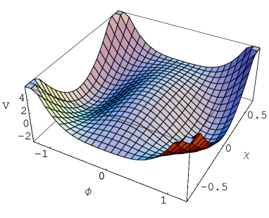
Figure 1: The shape of the scalar potential $V(\phi,\chi)$ for symmetric brane scenario. The parameters are set to $a=b=2$ and $v=1$.

It is very interesting that there exist degenerate Bloch brane solutions for $a=b$ and $a=4b$ DutraPLB2005 ; DegenerateBlochbranes . For the case $a=b$, the solution is DegenerateBlochbranes

$${\phi}(y) = v\frac{\sqrt{c_{0}^{2}-4}\sinh(2bvy)}{\sqrt{c_{0}^{2}-4}\cosh(2bvy)-c_{0}},$$ (10a)

$${\chi}(y) = \frac{2v}{\sqrt{c_{0}^{2}-4}\cosh(2bvy)-c_{0}},$$ (10b)

$$e^{2A(y)} = \bigg{(}\frac{\sqrt{c_{0}^{2}-4}-c_{0}}{\sqrt{c_{0}^{2}-4}\cosh(2bvy)-c_{0}}\bigg{)}^{4v^{2}/9}$$ (10c)

$$\times \exp\bigg{[}-\frac{4v^{2}\big{(}c_{0}^{2}-4-c_{0}\sqrt{c_{0}^{2}-4}\big{)}}{9\big{(}\sqrt{c_{0}^{2}-4}-c_{0}\big{)}^{2}}\bigg{]}$$

$$\times \exp\bigg{[}\frac{4v^{2}\big{(}c_{0}^{2}-4-c_{0}\sqrt{c_{0}^{2}-4}\cosh(2bvy)\big{)}}{9\big{(}\sqrt{c_{0}^{2}-4}\cosh(2bvy)-c_{0}\big{)}^{2}}\bigg{]},$$

where $c_{0}<-2$. For $a=4b$, one can get DegenerateBlochbranes

$${\phi}(y) = \frac{v\sqrt{1-16c_{0}}~{}\text{sinh}(4bvy)}{1+\sqrt{1-16c_{0}}~{}\cosh(4bvy)},$$ (11a)

$${\chi}(y) = \frac{2v}{\sqrt{1+\sqrt{1-16c_{0}}~{}\cosh(4bvy)}},$$ (11b)

$$e^{2A(y)} = \left(\frac{1+\sqrt{1-16c_{0}}}{1+\sqrt{1-16c_{0}}\cosh[4bvy]}\right)^{\frac{8v^{2}}{9}}$$ (11c)

$$\times \exp\left[\frac{{4v^{2}}\big{(}1+8c_{0}+\sqrt{1-16c_{0}}\big{)}}{9\big{(}1+\sqrt{1-16c_{0}}\big{)}^{2}}\right]$$

$$\times \exp\left[-\frac{{4v^{2}}\big{(}1+8c_{0}+\sqrt{1-16c_{0}}\cosh(4bvy)\big{)}}{9\big{(}1+\sqrt{1-16c_{0}}\cosh(4bvy)\big{)}^{2}}\right],$$

where $c_{0}<1/16$. The above two brane solutions (10) and (11) have similar properties, so we only focus on the solution (10) in this paper.

II.2 Asymmetric Bloch brane

Next, we construct asymmetric Bloch brane solutions by shifting the superpotential (8) a positive constant $W\rightarrow W+3\beta/2$. Note that the shift does not change the solutions for the scalars $\phi$ and $\chi$. The extrema of the new scalar potential are also at $\chi=0,~{}\phi=\pm v$. Now, the form of the warp factor exponent is changed to $A(y)-{\beta}y$ with $A(y)$ given by (7c), (9c),  (10c), (11c) for the four symmetric Bloch branes above, respectively. In order to have a finite value for $A(y)-{\beta}y$ at $y\rightarrow\pm\infty$, we need some limit on the parameter $\beta$, which turns out to be

$$|\beta|\leq\frac{4}{9}av^{3}$$ (12)

for all the solutions. The space-time far away from the brane is AdS₅ with different cosmological constants:

$$\Lambda_{\pm}=-\frac{1}{27}(9\beta\pm 4bv^{3})^{2}.$$ (13)

This is similar to the situation in Refs. Guerrero2006 ; MelfoPRD2006 . While the cosmological constant at the origin of the extra dimension has a slightly different expression:

$$\Lambda_{0}=\left\{\begin{array}[]{ll}\frac{1}{2}(a-3b)^{2}v^{4}-3\beta^{2}&~{}~{}\text{for~{}solution}~{}(\ref{BlochBrane2})\\ \frac{1}{2}b^{2}v^{4}\big{(}1-\frac{4}{(c_{0}-\sqrt{c_{0}^{2}-4})^{2}}\big{)}^{2}-3\beta^{2}&~{}~{}\text{for~{}solution}~{}(\ref{DBbrane1})\\ \frac{1}{2}b^{2}v^{4}\big{(}1-\frac{4}{1+\sqrt{1-16c_{0}}}\big{)}^{2}-3\beta^{2}&~{}~{}\text{for~{}solution}~{}(\ref{DBbrane2})\end{array}\right.,$$ (17)

which is positive for a symmetric brane scenario and can be positive, zero, or negative for an asymmetric scenario.

The shape of the energy density $\rho$ for the symmetric and asymmetric degenerate Bloch branes is shown in Figs. 2 and 3. The thickness of the degenerate branes could be estimated as

$$\delta=\left\{\begin{array}[]{ll}\frac{1}{bv}\ln\frac{-2c_{0}}{\sqrt{c_{0}^{2}-4}}&~{}~{}\text{for~{}solution}~{}(\ref{DBbrane1})~{}\text{with}~{}c_{0}\rightarrow-2\\ \frac{1}{2bv}\ln\frac{6}{\sqrt{1-16c_{0}}}&~{}~{}\text{for~{}solution}~{}(\ref{DBbrane2})~{}\text{with}~{}c_{0}\rightarrow 1/16\end{array}\right.,$$ (20)

It is clear that the single brane is localized at $z=0$, while the two sub-branes are localized at $z=\pm\delta/2$ and the thickness of the double brane is $\delta$. In what follows, we mainly discuss the solution (10) with the case $c_{0}\rightarrow-2$ (the double brane case); the discussion and result for (11) are similar. We define a new constant $u$ for convenience as

$$u=\sqrt{c_{0}^{2}-4}.$$ (21)

Then the double brane case corresponds to $u\rightarrow 0$ now, and we can further let

$$u=4~{}e^{-\delta_{0}}$$ (22)

with $\delta_{0}\gg 1$. The thickness of the double brane for solution (10) is

$$\delta\approx\frac{1}{bv}\ln\frac{4}{u}=\frac{\delta_{0}}{bv}.$$ (23)

Note that this thickness can be adjusted easily by $\delta_{0}$, an integral parameter independent of the scalar potential $V(\phi,\chi)$. Furthermore, the thickness is independent of the asymmetric factor $\beta$.

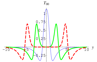
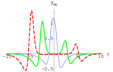
Figure 2: The shape of the energy density ($T_{00}$) for the symmetric ($\beta=0$, left) and asymmetric ($\beta=1/16$, right) degenerate Bloch branes with $a=b$. The parameters are set to $b=1,~{}v=1$, $c_{0}=-2-10^{-8}~{}(\delta_{0}=9.9)$ for the red dashed lines, $c_{0}=-2-10^{-4}~{}(\delta_{0}=5.3)$ for the green thick lines, and $c_{0}=-2.5$ for the blue thin lines.

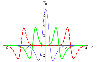
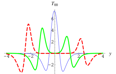
Figure 3: The shape of the energy density for the symmetric ($\beta=0$, left) and asymmetric ($\beta=1/16$, right) degenerate Bloch branes with $a=4b$. The parameters are set to $b=1,~{}v=1$, $c_{0}=\frac{1}{16+10^{-6}}(\delta_{0}=5.0)$ for the red dashed lines, $c_{0}=\frac{1}{16+10^{-2}}(\delta_{0}=2.7)$ for the green thick lines, and $c_{0}=0.01$ for the blue thin lines.

III The zero mode and resonances of gravity on the Bloch branes

Stability and zero mode of gravity on the symmetric Bloch brane have been analyzed in Ref. DegenerateBlochbranes . Here we further analyze the zero mode and resonances of gravity on the symmetric and asymmetric Bloch branes corresponding to the solution (10), which is rewritten as follows:

$${\phi}(y) = \frac{uv\sinh(2bvy)}{u\cosh(2bvy)-c_{0}},$$ (24a)

$${\chi}(y) = \frac{2v}{u\cosh(2bvy)-c_{0}},$$ (24b)

$$e^{2A(y)} = \left(\frac{c_{0}-u}{c_{0}-u\cosh(2bvy)}\right)^{4v^{2}/9}\exp{(-2\beta y)}$$ (24c)

$${\times} \exp{\left[\frac{4uv^{2}}{9}\left(\frac{u-c_{0}\cosh(2bvy)}{(c_{0}-u\cosh(2bvy))^{2}}-\frac{1}{u-c_{0}}\right)\right]}.$$

We will analyze the spectra of gravity on the thick brane by presenting the potential of the corresponding Schrödinger-like equation of the gravitational KK modes. In order to obtain the corresponding mass-independent potential, we perform the coordinate transformation

$$dz=e^{-A(y)}dy$$ (25)

to get a conformally flat metric

$$ds^{2}=e^{2A(z)}(\eta_{\mu\nu}dx^{\mu}dx^{\nu}+dz^{2}).$$ (26)

The analyzing of a full set of fluctuations of the metric around the background is a complex work. However, the problem can be simplified when one only considers the transverse and traceless part of the metric fluctuation dewolfe . So, we consider the following tensor perturbation of the metric:

$$ds^{2} = \left(e^{2A(z)}\eta_{\mu\nu}+\hat{h}_{\mu\nu}(x,z)\right)dx^{\mu}dx^{\nu}+e^{2A(z)}dz^{2}$$ (27)

$$= e^{2A(z)}\left[\left(\eta_{\mu\nu}+h_{\mu\nu}(x,z)\right)dx^{\mu}dx^{\nu}+dz^{2}\right].$$

Here $h_{\mu\nu}$ is the tensor perturbation of the metric, and it satisfies the transverse traceless condition dewolfe : ${h_{\mu}}^{\mu}=\partial^{\nu}h_{\mu\nu}=0$. The equation for $h_{\mu\nu}$ is given by

$$\partial_{z}^{2}h_{\mu\nu}+3(\partial_{z}A)(\partial_{z}h_{\mu\nu})+\eta^{\lambda\rho}\partial_{\lambda}\partial_{\rho}h_{\mu\nu}=0.$$ (28)

By performing the following decomposition

$$h_{\mu\nu}(x,z)=e^{-\frac{3}{2}A}e^{ikx}\varepsilon_{\mu\nu}h(z),$$ (29)

where $k^{2}=-m^{2}$ with $m$ the four-dimensional mass of a gravitational KK excitation, Eq. (28) can be recast into a Schrödinger-like equation

$$\big{(}-\partial_{z}^{2}+V_{G}(z)\big{)}h(z)=m^{2}h(z)$$ (30)

with the effective potential given by

$$V_{G}(z)=\frac{3}{2}\partial_{z}^{2}A(z)+\frac{9}{4}\big{(}\partial_{z}A(z))^{2}.$$ (31)

III.1 The potential and the zero mode

Here, we face the difficulty that the function $y(z)$ cannot be expressed in an explicit form for the brane solutions given in the previous section. But we can write the potential $V_{G}$ as a function of $y$:

$$V_{G}(z(y)) = e^{2A(y)}\bigg{(}\frac{3}{2}\partial_{y}^{2}A(y)+\frac{15}{4}\big{(}\partial_{y}A(y)\big{)}^{2}\bigg{)}.$$ (32)

For the asymmetric brane solution corresponding to (24), the explicit expression of $V_{G}(z(y))$ is

$$V_{G}(z(y)) = \left(\frac{c_{0}-u}{c_{0}-u{\cosh}(2bvy)}\right)^{\frac{4v^{2}}{9}}\exp\left[\frac{4}{9}uv^{2}\left(\frac{u-c_{0}\cosh(2bvy)}{\left(c_{0}-u\cosh(2bvy)\right)^{2}}-\frac{1}{u-c_{0}}\right)-2{\beta}y\right]$$ (33)

$$\times \left\{\frac{5}{108}\left[2bu^{2}v^{3}{\sinh}(2bvy)\frac{\left(u(5+{\cosh}(4bvy))-6c_{0}{\cosh}(2bvy)\right)}{\left(u{\cosh}(2bvy)-c_{0}\right)^{3}}+9\beta\right]^{2}\right.$$

$$~{}~{}~{}+\left.2b^{2}u^{2}v^{4}\frac{\left(4uc_{0}{\cosh}(2bvy)-\left(c_{0}^{2}+4\right){\cosh}(4bvy)-3u^{2}\right)}{\left(u{\cosh}(2bvy)-c_{0}\right)^{4}}\right\}.$$

The values of $V_{G}$ at $y=0$ and $y\rightarrow\pm\infty$ are

$$V_{G}(0)=\frac{15\beta^{2}}{4}-\frac{8b^{2}v^{4}u^{2}(2+u^{2}+u\sqrt{u^{2}+4})}{(u+\sqrt{u^{2}+4})^{4}},$$ (34)

$$V_{G}(y\rightarrow\pm\infty)\rightarrow 0.$$ (35)

The corresponding zero mode solution is

$$h_{0}(z(y)) \propto e^{\frac{3}{2}A(z(y))}=h^{S}_{0}(z(y))\;e^{-\frac{3}{2}\beta y},$$ (36)

where $h^{S}_{0}(z(y))$ is the zero mode solution for the symmetric brane case and is given by

$$h^{S}_{0}(z(y)) \propto \left(\frac{c_{0}-u}{c_{0}-u{\cosh}(2bvy)}\right)^{{v^{2}}/{3}}$$ (37)

$$\times \exp\left\{\frac{uv^{2}(u-c_{0}{\cosh}(2bvy))}{3\left(c_{0}-u{\cosh}(2bvy)\right)^{2}}\right\}.$$

For small $u=\sqrt{c_{0}^{2}-4}\ll 1$, the brane has two sub-branes (see Fig. 2) and the potential $V_{G}$ has two subwells located at $y=\pm\delta/2$ (see Fig. 4). The zero mode $h_{0}(z(y))$ is a constant between the two sub-branes for the symmetric brane and it is localized on the left sub-brane for the asymmetric brane. The zero mode represents the four-dimensional graviton; it is also the lowest energy eigenfunction (ground state) of the Schrödinger-like equation (30) since it has no zeros. Since the ground state has the lowest mass square $m_{0}^{2}=0$, there is no tachyonic gravitational KK mode.

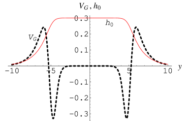
(a) $\beta=0$

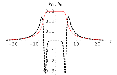
(b) $\beta=0$

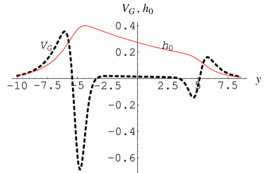
(c) $\beta=1/16$

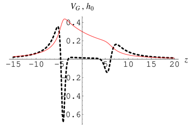
(d) $\beta=1/16$

Figure 4: The shape of the potential $V_{G}$ (thick dashed lines) and the zero mode $h_{0}$ (red thin lines) for the symmetric (up) and asymmetric (down) degenerate Bloch branes with $a=b$ in $y$ (left) and $z$ (right) coordinates. The parameters are set to $b=v=1$, $c_{0}=-2-10^{-8}~{}(\delta_{0}=9.9)$.

III.2 The massive KK modes and the resonances of gravity on the symmetric Bloch brane

Since $V_{G}(z)\rightarrow 0$ when $z\rightarrow\pm\infty$, the potential provides no mass gap to separate the gravitational zero mode from the excited KK modes; i.e., there exists a continuous gapless spectrum of the KK modes. The massive modes will propagate along the extra dimension and those with lower energy will experience an attenuation due to the presence of the potential barriers near the location of the brane.

The shape of the potential is strongly dependent on the constant $u$ (or $c_{0}$). When $u\rightarrow 0$, two subwells around the corresponding two sub-brane locations would appear, which could be related to gravitational resonances. In Refs. GremmPLB2000 ; 0801.0801 , the authors found that there exist gravitational resonances on the thick domain wall, and the resonances could remarkably affect the modifications of the four-dimensional Newton’s law at distances 0801.0801 . In Refs. 0901.3543 ; Liu0904.1785 ; Liu0907.0910 , a similar potential and resonances for left- and right-handed fermions were also found on thick branes with and without internal structure. In what follows, we investigate the massive modes of gravity by solving numerically Eq. (30) with potential in (33). We follow the method presented in Ref. Liu0904.1785 to calculate the probability for finding the massive modes on the Bloch brane.

We impose two kinds of initial conditions in order to obtain the solutions of the KK modes $h(z)$ from the second-order differential equations (30):

$$h(0)=h_{0},h^{\prime}(0)=0,$$ (38)

and

$$h(0)=0,~{}~{}h^{\prime}(0)=h_{1}.$$ (39)

The first and second conditions would result in even and odd KK modes for symmetric potential, respectively. The constants $h_{0}$ and $h_{1}$ for unbound massive KK modes are arbitrary. The massive KK modes would encounter the tunneling process across the potential barriers near the brane. And the modes with different masses would have different lifetimes.

One can interpret $|h(z)|^{2}$ as the probability for finding the massive KK modes at the position $z$ along extra dimension 0901.3543 . According to Refs. Liu0904.1785 ; Liu0907.0910 , large relative probabilities for finding massive KK modes within a narrow range $-z_{b}<z<z_{b}$ around the brane location, called $P_{G}$, would indicate the existence of resonances. The relative probabilities could be defined in a box with borders $|z|=10z_{b}$ as follows Liu0904.1785 :

$$P_{G}(m)=\frac{\int_{-z_{b}}^{z_{b}}|h(z)|^{2}dz}{\int_{-10z_{b}}^{10z_{b}}|h(z)|^{2}dz}.$$ (40)

Note that the KK mode with mass square $m^{2}$ much larger than the maximum of the corresponding potential $V_{G}^{max}$, i.e., $m^{2}\gg V_{G}^{max}$, can be approximated as a plane wave mode $h(z)\propto\cos mz$ or $\sin mz$, and the corresponding probability would trend to 0.1.

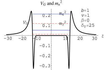
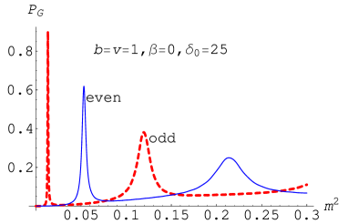
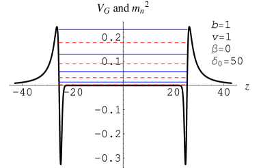
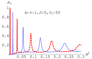
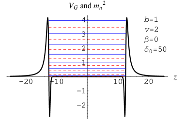
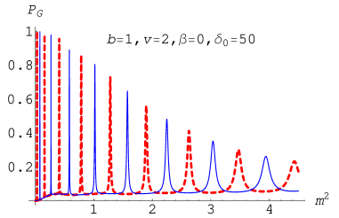
Figure 5: The potential $V_{G}(z)$, the resonance spectrum $m_{n}^{2}$ and the probability $P_{G}(m^{2})$ of the gravitational KK modes $h(z)$. In the figures of $V_{G}(z)$ and $m_{n}^{2}$, $V_{G}(z)$ is denoted by black thick lines, $m_{n}^{2}$ for the odd resonance KK mode is denoted by red dashed lines, and $m_{n}^{2}$ for the even resonance KK mode is denoted by blue thin lines. In the figures of $P_{G}(m^{2})$, the curves of $P_{G}(m^{2})$ for odd and even modes $h(z)$ are denoted by red dashed lines and blue thin lines, respectively.

We investigate the massive KK modes of gravity by solving numerically Eq. (30). For the set of parameters $a=b=1,v=1,~{}\beta=0$, and $\delta_{0}=25~{}($i.e., $c_{0}=-2-7.71\times 10^{-22})$, we find four peaks located at $m^{2}=\{0.0134$, $0.0533$, $0.1195$, $0.2137\}$ for the KK modes of gravity (see Fig. 5). These peaks are related with resonances of gravity, which are long-lived massive gravitational excitations on the brane. Except several peaks, the curves grow at first, and then stably trend to $z_{b}/z_{max}=0.1$. The reason is that KK modes with small $m^{2}(\ll V_{G}^{max})$ will be damped near the brane and oscillate away from the brane, while those modes with large $m^{2}(\gg V_{G}^{max})$ can be approximated as plane wave modes $h(z)\propto\cos mz$ or $\sin mz$. Note that any gravitational excitation with $m^{2}>0$ produced on the brane cannot correspond exactly to a single resonant KK mode because it has a wave function truly localized on the brane mass5-Dscalar . It is a wave packet composed of the continuum modes with a Fourier spectrum peaked around one of the resonances.

For $a=b=1,v=1,~{}\beta=0$, and $\delta_{0}=50$, i.e., a brane with double width compared to the one with the same values of $a,~{}b,~{}v,~{}\beta$ but $\delta_{0}=25$, we find eight resonances for gravity, and the mass spectrum of the resonances is calculated as

$$m^{2} = \{0.0029,0.0138,0.0318,0.0570,0.0895,$$ (41)

$$~{}0.1293,0.1765,0.2313\}.$$

For $a=b=1,v=2,~{}\beta=0$, and $\delta_{0}=50$, i.e., a brane with the same width compared to the one with $a=b=1,v=1,~{}\beta=0$, and $\delta_{0}=50$, we find sixteen resonances with the mass spectrum given by

$$m^{2} = \{0.0283,0.0777,0.1572,0.2676,0.4091,0.5815,$$ (42)

$$~{}0.7850,1.0180,1.2814,1.5748,1.8968,2.2492,$$

$$~{}2.6283,3.0389,3.4731,3.9435\}.$$

We can see that the number of the resonances increases with the width of the double brane and the value of $v$, which is related with the VEV of the scalar $\phi$. The potential $V_{G}(z)$, the resonance spectra $m_{n}^{2}$ and the probability $P_{G}(m^{2})$ of the gravitational KK mode $h_{n}(z)$ are shown in Fig. 5. Figure. 6 shows the lower level resonance KK modes of gravity. The $n=0$ level mode is in fact the only one bound state, namely, the four-dimensional massless graviton $h_{0}$.

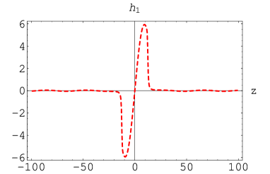
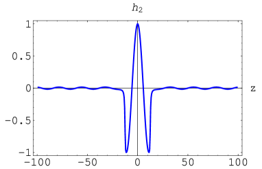
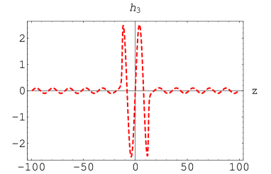
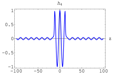
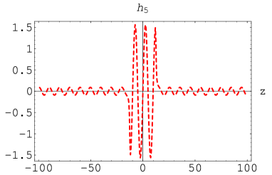
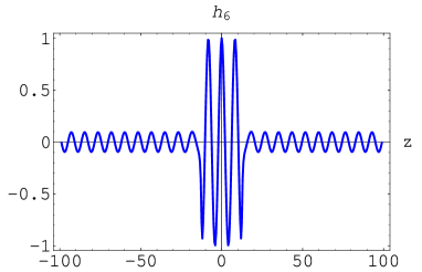
Figure 6: The lower level ($n=~{}1-6$) resonance KK modes $h_{n}(z)$ of gravity with the parameters set as $a=b=1,v=2,~{}\beta=0$ and $\delta_{0}=50$. The odd and even resonance KK modes are denoted by the red dashed lines and the blue continuous lines, respectively.

III.3 The resonances of gravity on the asymmetric Bloch brane

In this subsection, we will calculate the resonances of gravity on the asymmetric Bloch brane. Now the effective potential is asymmetric, so the corresponding KK modes have no definite parity anymore. Therefore, the relative probability method used in the last subsection is not convenient for the asymmetric case here. We will adopt the transfer matrix method first introduced in Ref. Landim2011 and subsequently used in Refs. Landim2012 ; Alencar2012 ; zhao2013 . In order to check the consistency of the two methods, we will first calculate the resonances of gravity on the symmetric Bloch brane with the transfer matrix method. Then we will apply it to the asymmetric case.

In this method, the interval of extra dimension, outside of which the potential is small enough, is divided into $N$ intervals with enough large $N$, and the coordinate is denoted by $z_{0},z_{1},\cdots,z_{N}$. In each interval the potential is replaced by a square potential barrier $V_{i}$ and the Schrödinger-like equation is solved. Then with the continuity of the KK modes and their first derivatives at each point $z_{i}$ and the iterative method, one can lastly get the transmission coefficient $T$ zhao2013 :

$$T=\frac{k_{1}}{k_{N}}\frac{1}{\mid M_{22}\mid^{2}}=\sqrt{\frac{\mid V_{1}-E_{n}\mid}{\mid V_{N}-E_{n}\mid}},$$ (43)

where $E_{n}=m_{n}^{2}$ is the “energy” of the particle, and $M$ is the product of the $N$ transfer coefficient matrixes $M_{i}$ with dimension $2\times 2$. Note that the transmission coefficient $T$ (43) for a symmetric potential (for which $V_{1}=V_{N}$ for a symmetric coordinate interval) will reduce to the one given in Ref. Landim2011 : $T={1}/{\mid M_{22}\mid^{2}}$.

For a given potential, the transmission coefficient $T$ is dependent on the value of the mass square $m^{2}$. So it can be considered as a function of $m^{2}$, like the case of $P(m^{2})$. If $T(m^{2})$ has a peak at some $m^{2}$, then we will have a higher probability to find this massive KK mode on the brane, and we will call this KK mode a resonant state. This is coincident with the relative probability method, which can be seen from Figs. 5 and  7. In Fig. 7, each peak corresponds to a resonant KK state. For the symmetric potential case, the transmission coefficient for each resonance is almost 1. Those resonances with smaller mass square have sharper resonance peaks, which is similar to the results of the relative probability method obtained in the last subsection.

The asymmetric case is shown in Fig. 8. We note here that the resonant KK modes should only correspond to those peaks with mass square smaller than the small maximum of the asymmetric potential, which is respectively 0.2, 0.16, and 0.1 for the three potentials plotted in Fig. 8, because for massive KK modes, there is a “quasipotential well” that can trap these KK modes at a finite time. The lifetime can also be estimated from the half-width of the peak. The numerical results show that the number and the transmission coefficients of the resonant KK modes will decrease with the asymmetric factor $\beta$. For larger enough asymmetric factor, there will no quasipotential well and hence no resonance anymore, even though there is still a resonance structure in the $T-m^{2}$ picture. On the other hand, we can see that for a potential, the resonance with smaller mass square has a longer lifetime, which is the same as the symmetric brane case.

Figure 7: The potential $V_{G}(z)$ and the transmission coefficient $T_{G}$ of gravity KK modes on the symmetric Bloch brane.

Figure 8: The potential $V_{G}(z)$ and the transmission coefficient $T_{G}$ of gravity KK modes on the asymmetric Bloch brane.

IV Localization and mass spectra of fermions on the Bloch brane

In this section, we would like to investigate the localization problem of fermions on the symmetric and asymmetric thick branes given in Eqs. (24) by introducing scalar-fermion coupling. We will analyze the spectra of fermions on the thick brane by presenting the potential of the Schrödinger-like equation of the fermion KK modes.

In five dimensions, fermions are four-component spinors and their Dirac structure is described by $\Gamma^{M}=e^{M}_{\bar{M}}\Gamma^{\bar{M}}$ with $\{\Gamma^{M},\Gamma^{N}\}=2g^{MN}$, where $\bar{M},\bar{N},\cdots=0,1,2,3,5$ denote the five-dimensional local Lorentz indices, and $\Gamma^{\bar{M}}$ are the flat gamma matrices in five dimensions. In our setup, $\Gamma^{M}=(\text{e}^{-A}\gamma^{\mu},\text{e}^{-A}\gamma^{5})$, where $\gamma^{\mu}$ and $\gamma^{5}$ are the usual flat gamma matrices in the Dirac representation. The Dirac action of a massless spin-1/2 fermion coupled to the scalar is

$$S_{1/2}=\int d^{5}x\sqrt{-g}\left(\bar{\Psi}\Gamma^{M}D_{M}\Psi-\eta\bar{\Psi}F(\phi)\Psi\right),$$ (44)

where the covariant derivative $D_{M}$ is defined as $D_{M}\Psi=(\partial_{M}+\omega_{M})\Psi$ with the spin connection $\omega_{M}=\frac{1}{4}\omega_{M}^{\bar{M}\bar{N}}\Gamma_{\bar{M}}\Gamma_{\bar{N}}$. With the metric (2), the nonvanishing components of the spin connection $\omega_{M}$ are

$$\omega_{\mu}=\frac{1}{2}(\partial_{z}A)\gamma_{\mu}\gamma_{5}.$$ (45)

Then the five-dimensional Dirac equation is read as

$$\left[\gamma^{\mu}\partial_{\mu}+\gamma^{5}\left(\partial_{z}+2\partial_{z}A\right)-\eta\;\text{e}^{A}F(\phi)\right]\Psi=0,$$ (46)

where $\gamma^{\mu}\partial_{\mu}$ is the Dirac operator on the brane. Note that the sign of the coupling $\eta$ between the spinor $\Psi$ and the scalar $\phi$ is arbitrary and represents a coupling either to kink or to antikink domain wall. For definiteness, we will consider in what follows only the case of a kink coupling, and thus assume that $\eta>0$.

Now we study the above five-dimensional Dirac equation. Because of the Dirac structure of the fifth gamma matrix $\gamma^{5}$, we expect the left- and right-handed projections of the four-dimensional part to behave differently. From the equation of motion (46), we will search for the solutions of the general chiral decomposition

$$\Psi(x,z) = \sum_{n}\Big{(}\psi_{Ln}(x)\hat{f}_{Ln}(z)+\psi_{Rn}(x)\hat{f}_{Rn}(z)\Big{)},$$ (47)

$$= \text{e}^{-2A}\sum_{n}\Big{(}\psi_{Ln}(x)f_{Ln}(z)+\psi_{Rn}(x)f_{Rn}(z)\Big{)},$$

where $\hat{f}_{L,R}(z)=\text{e}^{-2A}{f}_{L,R}(z)$, $\psi_{Ln}(x)=-\gamma^{5}\psi_{Ln}(x)$ and $\psi_{Rn}(x)=\gamma^{5}\psi_{Rn}(x)$ are the left-handed and right-handed components of a four-dimensional Dirac field, respectively, the sum over $n$ can be both discrete and continuous. Here, we assume that $\psi_{Ln}(x)$ and $\psi_{Rn}(x)$ satisfy the four-dimensional massive Dirac equations $\gamma^{\mu}\partial_{\mu}\psi_{Ln}(x)=m_{n}\psi_{R_{n}}(x)$ and $\gamma^{\mu}\partial_{\mu}\psi_{Rn}(x)=m_{n}\psi_{L_{n}}(x)$. Then $f_{Ln}(z)$ and $f_{Rn}(z)$ satisfy the following coupled equations

$$\left[\partial_{z}+\eta\;\text{e}^{A}F(\phi)\right]f_{Ln}(z) = +m_{n}f_{Rn}(z),$$ (48a)

$$\left[\partial_{z}-\eta\;\text{e}^{A}F(\phi)\right]f_{Rn}(z) = -m_{n}f_{Ln}(z).$$ (48b)

From the above coupled equations, we get the Schrödinger-like equations for the KK modes of the left- and right-handed fermions

$$\big{(}-\partial^{2}_{z}+V_{L}(z)\big{)}f_{Ln} = \mu_{n}^{2}f_{Ln},$$ (49a)

$$\big{(}-\partial^{2}_{z}+V_{R}(z)\big{)}f_{Rn} = \mu_{n}^{2}f_{Rn},$$ (49b)

where the effective potentials are given by

$$V_{L}(z) = \big{(}\eta\;\text{e}^{A}F(\phi)\big{)}^{2}-\partial_{z}\big{(}\eta\;\text{e}^{A}F(\phi)\big{)},$$ (50a)

$$V_{R}(z) = V_{L}(z)|_{\eta\rightarrow-\eta}.$$ (50b)

In order to obtain the standard four-dimensional action for the massive chiral fermions:

$$S_{1/2} = \int d^{5}x\sqrt{-g}~{}\bar{\Psi}\left(\Gamma^{M}(\partial_{M}+\omega_{M})-\eta F(\phi)\right)\Psi$$ (51)

$$= \sum_{n}\int d^{4}x\left(~{}\bar{\psi}_{Rn}\gamma^{\mu}\partial_{\mu}\psi_{Rn}-~{}\bar{\psi}_{Rn}m_{n}\psi_{Ln}\right)$$

$$+ \sum_{n}\int d^{4}x\left(~{}\bar{\psi}_{Ln}\gamma^{\mu}\partial_{\mu}\psi_{Ln}-~{}\bar{\psi}_{Ln}m_{n}\psi_{Rn}\right)$$

$$= \sum_{n}\int d^{4}x~{}\bar{\psi}_{n}(\gamma^{\mu}\partial_{\mu}-m_{n})\psi_{n},$$

we need the following orthonormality conditions for $f_{L_{n}}$ and $f_{R_{n}}$:

$$\int_{-\infty}^{\infty}f_{Lm}f_{Ln}dz=\delta_{mn}=\int_{-\infty}^{\infty}f_{Rm}f_{Rn}dz,~{}~{}$$

$$\int_{-\infty}^{\infty}f_{Lm}f_{Rn}dz=0.$$ (52)

It can be seen that, in order to localize the left- or right-handed fermions, there must be some kind of scalar-fermion coupling, and the effective potential $V_{L}(z)$ or $V_{R}(z)$ should have a minimum at the location of the brane. Furthermore, for the kink configuration of the scalar $\phi(z)$ (24a), $F(\phi(z))$ should be an odd function of $\phi(z)$ when one demands that $V_{L,R}(z)$ are invariant under $Z_{2}$ reflection symmetry $z\rightarrow-z$. Thus we have $F(\phi(0))=0$ and $V_{L}(0)=-V_{R}(0)=-\eta\partial_{z}(e^{A}F(\phi(0)))$, which results in the well-known conclusion: only one of the massless left- and right-handed fermions could be localized on the brane. The spectra are determined by the behavior of the potentials at infinity. For $V_{L,R}\rightarrow 0$ as $|z|\rightarrow\infty$, one of the potentials would have a volcanolike shape and there exists only a bound massless mode followed by a continuous gapless spectrum of KK states, while another could not trap any bound states and the spectrum is also continuous and gapless. The Yukawa coupling $F(\phi)=\phi$ and the generalized coupling $F(\phi)=\phi^{k}$ with positive odd integer $k\;(\geq 3)$ belong to this type. For $V_{L,R}\rightarrow V_{\infty}=$ positive constant as $|z|\rightarrow\infty$, those modes with $m_{n}^{2}<V_{\infty}$ belong to a discrete spectrum and modes with $m_{n}^{2}>V_{\infty}$ contribute to a continuous one. If the potentials increase as $|z|\rightarrow\infty$, the spectrum is discrete. There are a lot of couplings for this case. The concrete behavior of the potentials is dependent on the function $F(\phi)$. In what follows, we will discuss in detail the Yukawa coupling $F(\phi)=\phi$.

IV.1 The potentials

We mainly consider the Yukawa coupling $\eta\bar{\Psi}\phi\Psi$, for which the explicit forms of the potentials (50) are

$$V_{L} = \eta\left(\frac{u-c_{0}}{u\cosh(2bvy)-c_{0}}\right)^{\frac{4v^{2}}{9}}\text{e}^{-2\beta y}$$ (53a)

$$\times\exp\left\{\frac{4uv^{2}}{9}\left(\frac{u-c_{0}\cosh(2bvy)}{(u\cosh(2bvy)-c_{0})^{2}}-\frac{1}{u-c_{0}}\right)\right\}$$

$$\times\bigg{\{}\frac{8bu^{3}v^{4}[u-c_{0}\cosh(2bvy)]\text{sinh}^{2}(2bvy)}{9\left(u\cosh(2bvy)-c_{0}\right)^{4}}$$

$$+\frac{u^{2}v^{2}(18b+4bv^{2}+9\eta)\text{sinh}^{2}(2bvy)}{9\left(u\cosh(2bvy)-c_{0}\right)^{2}}$$

$$+\frac{uv(\beta\text{sinh}(2bvy)-2bv\cosh(2bvy))}{\left(u\cosh(2bvy)-c_{0}\right)}$$

$$+\frac{4bu^{2}v^{4}c_{0}\text{sinh}^{2}(2bvy)}{9\left(u\cosh(2bvy)-c_{0}\right)^{3}}\bigg{\}},$$

$$V_{R} = V_{L}|_{\eta\rightarrow-\eta},$$ (53b)

for the symmetric (let $\beta=0$) and asymmetric brane solutions. The double thick brane corresponds to the case $c_{0}\rightarrow-2$ and $u=4e^{-\delta_{0}}$ with $\delta_{0}\gg 1$.

Both potentials have the asymptotic behavior: $V_{L,R}(y\rightarrow\pm\infty)\rightarrow 0$. The values of the potentials for left- and right-handed fermions at $y=0$ are given by

$$V_{L}(0)=-V_{R}(0)=-\frac{2uv^{2}b}{(u-c_{0})}\eta.$$ (54)

It is clear that, for a given coupling constant $\eta$, the values of the potentials for left- and right-handed fermions at $y=0$ are opposite. The parameter $u$ is positive, $c_{0}<-2$, and $b$ and $\eta$ can be positive and negative. Considering that the potentials of left- and right-handed fermion KK modes are partner potentials, we will only take the positive values of $b$ and $\eta$ without loss of generality. We recall that the brane is a single brane and a double brane for $u\gg 1~{}(|c_{0}|\gg 2)$ and $u\ll 1~{}(c_{0}\rightarrow-2)$, respectively. For the double brane case, the potentials at the location of the brane are

$$V_{L}(0)=-V_{R}(0)=-uv^{2}b\eta\approx 0.$$ (55)

The shapes of the potentials are shown in Fig. 9 for different values of $u$ or $\delta_{0}$. From the figure we see that $V_{L}(z)$ is a modified volcano type potential for the single brane scenario and has a well. While for the double brane case with $u\ll 1$, the corresponding potential $V_{L}(z)$ for left-handed fermions has a double well, and the potential $V_{R}(z)$ for right-handed fermions has a single well, which indicates that there may exist resonant (quasilocalized) KK modes of fermions. Hence, the shape of the potentials is relative to the inner structure of the brane, or equivalently, it depends partly on the warp factor $e^{2A}$, and partly on the configuration of the scalar $\phi$. The effect of other parameters to the potentials is shown in Figs. 10 and 11.

On the other hand, we note that $V_{L}(z)\rightarrow 0$ from above when $y\rightarrow\pm\infty$, so the potential for left-handed fermions provides no mass gap to separate the fermion zero mode from the excited KK modes. For right-handed fermions, the corresponding potential $V_{R}(z)\rightarrow 0$ when $z\rightarrow\pm\infty$, and $V_{R}(0)>0$ when $z=0$, and there is no bound right-handed fermion zero mode. In fact, this is a simple consequence of the fact that $V_{L}$ and $V_{R}$ are partner potentials. For both left- and right-handed fermions, there exists a continuous gapless spectrum of the KK modes.

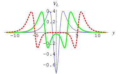
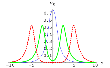
Figure 9: The shape of the potentials $V_{L,R}$ for the symmetric branes with $a=b$ for different values of $\delta_{0}$ in $y$ coordinates. The parameters are set to $b=1,~{}v=1,~{}\beta=0,~{}\eta=1$, $\delta_{0}=10~{}(u=0.00018)$ for the red dashed lines, $\delta_{0}=5~{}(u=0.027)$ for the green thick lines, and $\delta_{0}=1~{}(u=1.47)$ for the blue thin lines.

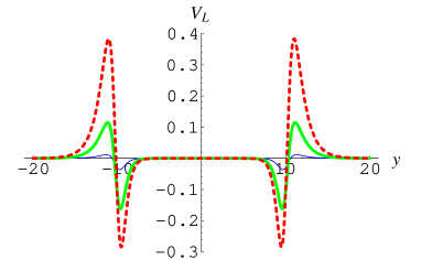
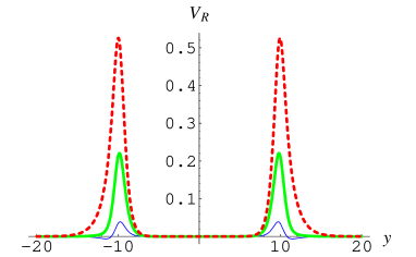
Figure 10: The shape of the potentials $V_{L,R}$ for the symmetric branes with $a=b$ for different Yukawa coupling constant $\eta$ in $y$ coordinates. The parameters are set to $b=1,~{}v=1,~{}\beta=0,~{}\delta_{0}=20~{}(u=8.2\times 10^{-9})$, $\eta_{0}=1$ for the red dashed lines, $\eta_{0}=0.5$ for the green thick lines, and $\eta_{0}=0.1$ for the blue thin lines.

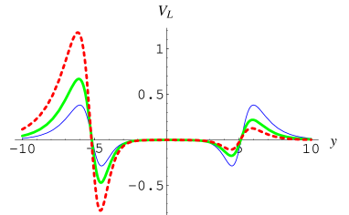
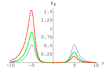
Figure 11: The shape of the potentials $V_{L,R}$ for the asymmetric branes with $a=b$ for different values of the asymmetric factor $\beta$ in $y$ coordinates. The parameters are set to $b=1,~{}v=1,~{}\eta=1,~{}\delta_{0}=10~{}(u=0.00018)$, $\beta_{0}=0.1$ for the red dashed lines, $\beta_{0}=0.05$ for the green thick lines, and $\beta_{0}=0$ for the blue thin lines.

IV.2 The zero mode

For positive $\eta$ and $b$, we will show that the potential for left-handed fermions could trap the left-handed fermion zero mode, which can be solved from (48a) by setting $m_{0}=0$:

$$f_{L0}(z)\propto\exp\left(-\eta\int^{z}_{0}dz^{\prime}\text{e}^{A(z^{\prime})}\phi(z^{\prime})\right).$$ (56)

In order to check whether the zero mode can be localized on the brane, we need to consider the normalizable problem of the solution. The normalization condition for the zero mode (56) is

$$\int_{-\infty}^{\infty}dz\exp\left(-2\eta\int^{z}_{0}dz^{\prime}e^{A(z^{\prime})}\phi(z^{\prime})\right)<\infty.$$ (57)

Since we do not know the analytic expressions of the functions $A(z)$ and $\phi(z)$ in $z$ coordinates, we have to deal with the problem in $y$ coordinates. With the relation (25), we can switch the normalization condition (57) to the following one in $y$ coordinates:

$$\int_{-\infty}^{\infty}dy\exp\left(-A(y)-2\eta\int^{y}_{0}dy^{\prime}\phi(y^{\prime})\right)<\infty.$$ (58)

Now, it is clear that, because $\exp(-A(y))$ is divergent at $y\rightarrow\pm\infty$, the introduction of the scalar-fermion coupling is necessary in order to localize the fermion zero mode on the brane. Since the functions $A(y)$ and $\phi(y)$ are smooth, the normalization of the zero mode is decided by the asymptotic characteristic of $\eta\phi(y)$ at $y\rightarrow\pm\infty$.

The integrand in (58) can be expressed explicitly as

$$I_{1} \propto \exp\bigg{[}-\frac{2uv^{2}(u-c_{0}\cosh(2bvy))}{9(u\cosh(2bvy)-c_{0})^{2}}+\beta y$$ (59)

$$~{}~{}~{}~{}~{}+\left(\frac{2v^{2}}{9}-\frac{\eta}{b}\right)\ln\left(u\cosh(2bvy)-c_{0}\right)\bigg{]}.$$

The asymptotic characteristic of $I_{1}$ at $y\rightarrow\pm\infty$ is

$$I_{1}\rightarrow\left\{\begin{array}[]{ll}\exp\left(-2v\big{(}\eta-\frac{2bv^{2}}{9}-\frac{\beta}{2v}\big{)}y\right)&~{}$when$~{}y\rightarrow+\infty\\ \exp\left(+2v\big{(}\eta-\frac{2bv^{2}}{9}+\frac{\beta}{2v}\big{)}y\right)&~{}$when$~{}y\rightarrow-\infty\end{array}\right..$$ (62)

So, the normalization condition of the zero mode turns out to be

$$\eta>\frac{2bv^{2}}{9}+\left|\frac{\beta}{2v}\right|,$$ (63)

which is simplified for the symmetric brane as $\eta>{2bv^{2}}/{9}$. Provided the condition (63), the zero mode of left-handed fermions can be localized on the brane. It can be seen that in order for the potential $V_{L}$ to localize the zero mode of left-handed fermions for larger $v$, $b$ or the asymmetric factor $\beta$, the stronger scalar-fermion coupling constant $\eta$ is required. That is to say, the massless mode of left-handed fermion is easier to be localized on the symmetric brane, and the asymmetric factor $\beta$ makes it more difficult to localize the zero mode. A similar result was also found in Ref. Liu0907.0910 . However, this is different from the situation of the zero modes of scalars and vectors on symmetric and asymmetric de Sitter branes LiuJCAP2009 , where increasing the asymmetric factor does not change the number of the bound vector KK modes but would increase that of the bound scalar KK modes, and the zero modes of scalars and vectors are always localized on the de Sitter branes. In Refs. KoleyCQG2005 ; LiuPRD2008 , it was shown that the zero mode of left-handed fermions can also be localized on the brane in the background of Sine-Gordon kinks provided similar condition as (63). The fermion zero mode cannot be localized on the de Sitter brane with the same coupling $F(\phi)=\phi$ LiuJCAP2009 .

The zero mode (56) can be explicitly written as a function of $y$:

$$f_{L0}(z(y))\propto\big{[}u\cosh(2bvy)-c_{0}\big{]}^{-\frac{\eta}{2b}}.$$ (64)

We note here that, although the zero mode $f_{L0}$ is an even function in the $y$ coordinate, it is asymmetric in the $z$ coordinate for the asymmetric brane because of the asymmetric warp factor. In Fig. 12, we plot the left-handed fermion potential $V_{L}$ and the corresponding zero mode for the symmetric and asymmetric branes in both the $y$ and $z$ coordinates. We see that the zero mode is bound on the branes. It represents the ground state of the Schrödinger-like equation (49a) since it has no zero. Since the ground state has the lowest mass square $m_{0}^{2}=0$, there is no tachyonic left-handed fermion mode. In fact, the differential equations (49a) and (49b) can be factorized as

$$\left[-\partial_{z}+\eta\;\text{e}^{A}F(\phi)\right]\left[\partial_{z}+\eta\;\text{e}^{A}F(\phi)\right]f_{Ln}(z) = m_{n}^{2}f_{Ln}(z),$$ (65)

$$\left[-\partial_{z}-\eta\;\text{e}^{A}F(\phi)\right]\left[\partial_{z}-\eta\;\text{e}^{A}F(\phi)\right]f_{Rn}(z) = m_{n}^{2}f_{Rn}(z).$$ (66)

It can be shown that $m_{n}^{2}$ is zero or positive since the resulting Hamiltonian can be factorized as the product of two operators which are adjoints of each other. Hence the system is stable.

The zero mode $f_{L0}$ on both the symmetric and asymmetric double branes is essentially constant between the two sub-branes. This is different from the case of gravity, where the gravitational zero mode $h_{0}$ on the asymmetric double brane is strongly localized on the sub-brane centered around the lower minimum of the potential. In Ref. Liu0907.0910 , fermions on one-field-generating symmetric and asymmetric double branes were also studied, where the asymmetric brane solution was constructed from a symmetric one with another method presented in asymdSBrane2 . It was found that the corresponding fermion zero mode $f_{L0}$ on both the double branes for the same Yukawa coupling $F(\phi)=\phi$ is also constant between the two sub-branes.

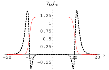
(a) $\beta=0$

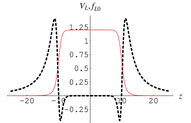
(b) $\beta=0$

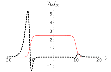
(c) $\beta=1/16$

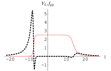
(d) $\beta=1/16$

Figure 12: The potential $V_{L}$ (thick dashed lines) and the fermion zero mode $f_{L0}$ (red thin lines) for the symmetric ($\beta=0$, up) and asymmetric ($\beta=1/16$, down) double branes with $a=b$ in $y$ (left) and $z$ (right) coordinates. The parameters are set to $b=1,~{}v=1,~{}\delta_{0}=20,~{}\eta=2$.

IV.3 The massive KK modes and the resonances

The massive modes will propagate along the extra dimension and those with lower energy would experience an attenuation due to the presence of the potential barriers near the location of the brane.

The potential $V_{R}$ is always positive near the brane location and vanishes when far away from the brane. This shows that it could not trap any bound fermions with right chirality and there is no zero mode of right-handed fermions. However, the shape of the potential is strongly dependent on the scalar-fermion coupling constant $\eta$. When $\eta$ increases to a certain value, the potential will appear as a quasiwell around the brane location and the quasiwell would become deeper and deeper, and as a result, this quasiwell will “trap” some fermions; in fact, they are called the quasilocalized or resonant fermions. Moreover, the number of resonances will increase with the scalar-fermion coupling constant $\eta$. In Ref. 0901.3543 , a similar potential and resonances for left- and right-handed fermions were found in background of two-field generated thick branes with internal structure, which demonstrates that a Dirac fermion could be composed from the left- and right-handed fermion resonance KK modes Liu0904.1785 .

We can investigate the massive modes of fermions by solving numerically Eqs. (49a) and (49b). For the set of parameters $b=v=1,~{}\beta=0,~{}\eta=2$ and $~{}\delta_{0}=20$, we find eight resonances located at $m^{2}=\{0.02704$, $0.1072$, $0.2379$, $0.41533$, $0.6346$, $0.89013$, $1.1766$, $1.4955\}$ for both left- and right-handed fermions (see Figs. 13(a) and 13(b)).

For $b=v=1,~{}\beta=0,~{}\eta=2$ and $~{}\delta_{0}=40$, i.e., a brane with double width compared to the one with the same values of $b,~{}v,~{}\beta,~{}\eta$ but $\delta_{0}=20$ (see Figs. 13(c) and 13(d)), we find sixteen resonances for right-handed fermions, and the mass spectrum of the resonances is calculated as

$$m^{2} = \{0.0065,0.0258,0.0580,0.1028,0.1602,0.2299,$$ (67)

$$~{}0.3116,0.4051,0.5100,0.6260,0.7524,$$

$$~{}0.8889,1.0350,1.1905,1.3559,1.5320\}.$$

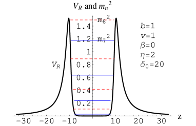
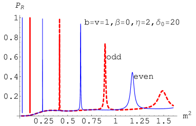
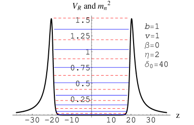
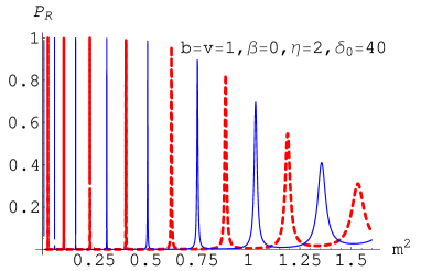
Figure 13: The potential $V_{R}(z)$, the resonance spectrum $m_{n}^{2}$, and the probability $P_{R}(m^{2})$ for the right-handed fermion KK modes $f_{Rn}$. In the figures of $V_{R}(z)$ and $m_{n}^{2}$, $V_{R}(z)$ is denoted by black thick lines; $m_{n}^{2}$ for the odd and even resonance KK modes $f_{Rn}$ are denoted by red dashed and blue thin lines, respectively. In the figures of $P_{R}(m^{2})$, the curves of $P_{R}(m^{2})$ for odd and even modes $f_{Rn}$ are also denoted by red dashed lines and blue thin lines, respectively.

We next analyze the lifetime of a fermion resonance. First, we define the width $\Gamma=\Delta m$ of each resonant state as the width at the half maximum of a resonant peak. In this case, a massive fermion will disappear into the fifth dimension after staying on the brane for some time $\tau\simeq\Gamma^{-1}$. Thus, $\tau$ is called the lifetime of a fermion resonance mentioned above. After numerical calculations, we get a lifetime from each peak of the fermion resonance, which is shown in detail in Fig. 14(a). We find that the first peak is the most narrow one; accordingly, the lifetime of this resonant state is the maximum, but it decays in exponential mode with the number $n$ increase, so we get the conclusion that the KK modes with a lower resonant state have a longer lifetime on the brane. However, for a certain resonant state and brane width, the lifetime increases with the larger coupling constant $\eta$. Also, from Fig. 14(b), we can see that the total resonance number $N$ increases with the coupling constant $\eta$ and it increases linearly with the width of the double brane $\delta$.

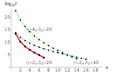
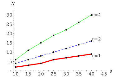
Figure 14: The relationship between $\text{log}_{10}\tau$ and $n$ (left), the total resonance number $N$ and the width of the double brane $\delta$ (right). Here $\tau$ denotes the lifetime of a fermion resonance, and $n$ labels the order of the resonances. The parameters are set to $b=1,~{}v=1,~{}\beta=0$.

We also use the transfer matrix method to calculate the resonance structure of fermion KK modes. For the symmetric case, the result is consistent with that of the relative possibility method, see Figs. 13 and 15. For the asymmetric case, the result is shown in Fig. 16. Note that the resonance structures for $\beta$ and $-\beta$ are the same, because the potentials for $\beta$ and $-\beta$ have the same shape. From Figs. 13 and 16, it can be seen that the the number and the transmission coefficients of the fermion resonant KK modes decrease with the asymmetric factor $\beta$ rapidly. For $\beta=0.01$, the transmission coefficients of the fermion resonant KK modes with mass square smaller than 1.25 are almost around 0.3. For a larger $\beta=0.02$, the transmission coefficients of those resonances within the quasipotential well decrease to 0.05, which is much less than 1, the value of the symmetric brane case. So the fermion resonance structure is more sensitive to the asymmetric factor than that of the gravity one.

Figure 15: The potential $V_{R}(z)$ and the transmission coefficient $T_{R}$ of right-handed fermion KK modes on the symmetric Bloch brane.

Figure 16: The potential $V_{R}(z)$ and the transmission coefficient $T_{R}$ of right-handed fermion KK modes on the asymmetric Bloch brane.

V Localization of the zero modes of the gravity and fermion on the asymmetric Bloch double brane

In Secs. III.1 and IV.2, we have investigated the zero modes of the gravity and fermion. However, the four-dimensional massless graviton and fermion are not denoted by $h_{0}(z)$ and $f_{0}(z)$, respectively. In fact, from the gravitational perturbation (27) of the metric, it can be seen that the real tensor perturbation of the metric is $\hat{h}_{\mu\nu}(x,z)$ but not $h_{\mu\nu}(x,z)$. Therefore, from Eqs. (27) and (29), it can be seen that the four-dimensional massless graviton is presented by

$$\hat{h}^{(0)}_{\mu\nu}(x,z)=e^{2A(z)}{h}^{(0)}_{\mu\nu}(x,z)=e^{ikx}\varepsilon_{\mu\nu}~{}e^{\frac{1}{2}A(z)}h_{0}(z),$$ (68)

and the localization of the four-dimensional massless graviton is characterized by $\hat{h}_{0}(z)=e^{\frac{1}{2}A(z)}{h}_{0}(z)$. Similarly, the four-dimensional massless fermions with left chirality and right chirality are presented by $\psi_{L0}(x)\hat{f}_{L0}(z)=e^{-2A(z)}\psi_{L0}(x){f}_{L0}(z)$ and $\psi_{R0}(x)\hat{f}_{R0}(z)=e^{-2A(z)}\psi_{R0}(x){f}_{R0}(z)$, respectively. Hence the localization of the four-dimensional massless fermions are characterized by $\hat{f}_{L0}(z)=e^{-2A(z)}{f}_{L0}(z)$ or $\hat{f}_{R0}(z)=e^{-2A(z)}{f}_{R0}(z)$.

The energy density $\rho$, the gravitational zero mode $\hat{h}_{0}$ and the fermion zero mode $\hat{f}_{L0}$ for the symmetric and asymmetric double branes are plotted in Fig. 17. By comparing Figs. 4, 12 and 17, we can find that the localization properties of four-dimensional massless graviton and fermion in the symmetric brane case read from two kinds of descriptions ($h_{0}$, $f_{L0}$ and $\hat{h}_{0}$, $\hat{f}_{L0}$) are the same; i.e., the graviton and the fermion are localized between the two sub-branes. However, for the asymmetric brane case, the results for the fermion caused by the two kinds of descriptions are not the same. As mentioned above, since the localization of the four-dimensional massless graviton and fermion should be described by $\hat{h}_{0}(z)$ and $\hat{f}_{L,R0}(z)$, respectively, we can conclude that the four-dimensional massless graviton is localized on the left sub-brane, while the four-dimensional massless fermion is localized on the right one.

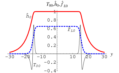
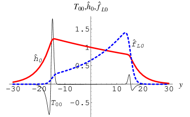
Figure 17: The energy density $T_{00}$ (the thin lines), the gravitational zero mode $\hat{h}_{0}$ (the thick red lines) and the fermion zero mode $\hat{f}_{L0}$ (the dashed blue lines) for the symmetric ($\beta=0$, left) and asymmetric ($\beta=1/9$, right) double branes in $y$ coordinates. The other parameters are set to $b=1,~{}v=1,~{}\eta=2,~{}\delta_{0}=20$. The zero modes $\hat{h}_{0}$ and $\hat{f}_{L0}$ are plotted with arbitrary normalization.

VI Discussions and conclusions

In this paper, by presenting the mass-independent potentials of the KK modes in the corresponding Schrödinger-like equations, we investigated the localization and mass spectra of gravity and spin-half fermion on symmetric and asymmetric thick branes. We found that the zero mode of gravity can be localized on the symmetric and asymmetric branes. For the case of fermion, there is no bound KK mode for both left- and right-handed fermion zero modes without scalar-fermion coupling ($\eta=0$). Hence, in order to localize the left- or right-handed massless fermion KK mode on the brane, some kind of Yukawa coupling should be introduced. In this paper, we considered the typical Yukawa coupling $\eta\bar{\Psi}\phi{\Psi}$, for which the localization conditions for the left-handed fermion zero modes are $\eta>\frac{2bv^{2}}{9}$ and $\eta>\frac{2bv^{2}}{9}+\left|\frac{\beta}{2v}\right|$ for the symmetric and asymmetric branes, respectively. So, it needs larger coupling constant in order to localize the fermion zero mode on the asymmetric brane. The zero mode of right-handed fermion cannot be localized on the brane at the same condition.

The spectra of the KK modes are determined by the behavior of the potentials at infinity. We found that all the potentials for the gravity and fermion KK modes turn to vanish at the boundary of extra dimension. Therefore, these potentials provide no mass gap to separate the zero modes from the excited KK modes. Consequently, the spectra of the gravity and the left- or right-handed fermion are composed of a bound zero mode and a series of gapless continuous massive KK modes.

For the case of a double brane, the potentials for the gravity and left-handed fermion KK modes almost vanish between the two sub-branes, and have two potential wells around the two sub-branes, while the potential for the right-handed fermion KK modes has a quasi potential well between the two sub-branes. For all of these potentials, there are two potential bars outside the two sub-branes. Such potentials result in some massive quasilocalized or resonant KK modes of gravity and fermion, which can stay on the branes for a certain time and then escape into the extra dimensions. The resonant state with lower mass has a longer lifetime on the brane. For the case of gravity, the number of the resonances increases with the width of the double brane and the VEV of the scalar $\phi$. For the case of left- and right-handed fermions, the lifetime of the $n$th resonance and the total number of the resonances increase with the scalar-fermion coupling constant $\eta$ and the width of the double brane. We found that the mass spectra of left- and right-handed fermion resonances are almost the same, which shows that a Dirac fermion with a finite lifetime on the brane could be composed of the left- and right-handed fermion resonance KK modes Liu0904.1785 .

For the asymmetric case, the fermion zero mode is localized on one of the sub-branes, while the gravity zero mode is localized on another sub-brane. The number and the transmission coefficients of the resonant KK modes of gravity of fermion will decrease with the asymmetric factor $\beta$. Just as in the symmetric brane case, the resonance with smaller mass square would have a longer lifetime. For a larger enough asymmetric factor, while there is still a resonance structure in the $T-m^{2}$ picture, it does not denote resonance anymore.

At last, we give a comment on an important but more complex issue about the scalar spin-0 modes of the model, which would determine if the brane setup is stable or not. This issue has been investigated in Refs. Shaposhnikov2005 ; George2011 ; Gherghetta2011 for one and $N$ real background scalar fields. It was found that the spin-0 degrees of freedom in the metric mix with the scalar perturbations. The zero modes of these perturbations were solved formally from the coupled Schrödinger equations, and they can be used to construct a solution matrix. With the eigenvalues of the solution matrix, one can judge if a normalizable zero mode exists or not and how many normalizable negative mass modes exist in the spectrum. The case of two scalars were discussed in detail in Ref. George2011 . According to Ref. George2011 , since the superpotential is used to generate the solution in our model, there may exist a scalar zero mode associated with the choice of integration constant(s) of the solutions in Eqs. (24). We will investigate this issue in future work.

Note-added. -Recently, we found another paper Cruz2013a that also considered the resonances of gravity on a Bloch brane.

VII ACKNOWLEDGMENT

We thank the referee for his/her crucial comments and suggestions, which helped us to improve the original manuscript. This work was supported by the National Natural Science Foundation of China (Grants No. 11075065 and 11375075), and the Fundamental Research Funds for the Central Universities (Grant No. lzujbky-2013-18).

References

- (1) T. Kaluza, Sitzungsber. Preuss. Akad. Wiss. Berlin, p. 966 (1921).
- (2) O. Klein, Z. Phys. 37, 895 (1926).
- (3) V.A. Rubakov and M.E. Shaposhnikov, Phys. Lett. 125 B, 136 (1983) .
- (4) K. Akama, Lect. Notes Phys. 176, 267 (1983).
- (5) I. Antoniadis, Phys. Lett. B 246, 377 (1990).
- (6) N. Arkani-Hamed, S. Dimopoulos, and G.R. Dvali, Phys. Lett. B 429, 263 (1998).
- (7) L. Randall and R. Sundrum, Phys. Rev. Lett. 83, 3370 (1999).
- (8) W.D. Goldberger and M.B. Wise, Phys. Rev. Lett. 83, 4922 (1999).
- (9) L. Randall and R. Sundrum, Phys. Rev. Lett. 83, 4690 (1999).
- (10) T. Gherghetta and A. Kehagiias, Phys. Rev. Lett. 90, 101601 (2003).
- (11) I. Antoniadis, A. Arvanitaki, S. Dimopoulos, and A. Giveon, Phys. Rev. Lett. 108, 081602 (2012).
- (12) Y.-X. Liu, Y. Zhong, Z.-H. Zhao, and H.-T. Li, J. High Energy Phys. 06(2011) 135 .
- (13) K. Yang, Y.-X. Liu, Y. Zhong, X.-L. Du, and S.-W. Wei, Phys. Rev. D 86, 127502 (2012).
- (14) O. DeWolfe, D.Z. Freedman, S.S. Gubser and A. Karch, Phys. Rev. D 62, 046008 (2000).
- (15) M. Gremm, Phys. Lett. B 478, 434 (2000).
- (16) C. Csaki, J. Erlich, T. Hollowood and Y. Shirman, Nucl. Phys. B 581, 309 (2000).
- (17) N. Barbosa-Cendejas, A. Herrera-Aguilar, M. A. ReyesSantos and C. Schubert, Phys. Rev. D 77, 126013 (2008).
- (18) Y.-X. Liu, Y. Zhong and K. Yang, Europhys. Lett. 90, 51001 (2010).
- (19) D.P. George, J. Phys. Conf. Ser. 259, 012034 (2010).
- (20) S. Mert Aybat and D.P. George, JHEP 1009, 010 (2010).
- (21) Z.-H. Zhao, Y.-X. Liu, and H.-T. Li, Class. Quant. Grav.27, 185001 (2010).
- (22) Z.-H. Zhao, Y.-X. Liu, H.-T. Li and Y.-Q. Wang, Phys. Rev. D 82, 084030 (2010).
- (23) Y. Zhong, Y.-X. Liu, and K. Yang, Phys. Lett. B 699, 398 (2011).
- (24) D. Bazeia, F.A. Brito, and F.G. Costa, Phys. Rev. D 87, 065007 (2013).
- (25) V. Dzhunushaliev, V. Folomeev and M. Minamitsuji, Rept. Prog. Phys. 73, 066901 (2010).
- (26) S. Randjbar-Daemi and M. Shaposhnikov, Phys. Lett. B 492, 361 (2000).
- (27) T.R. Slatyer and R.R. Volkas, JHEP 0704, 062 (2007).
- (28) Y.-X. Liu, X.-H. Zhang, L.-D. Zhang and Y.-S. Duan, JHEP 0802, 067 (2008).
- (29) D. Bazeia, F.A. Brito and R.C. Fonseca, Eur. Phys. J. C 63, 163 (2009).
- (30) C.-E. Fu, Y.-X. Liu, and H. Guo, Phys. Rev. D 84, 044036 (2011).
- (31) Y.-X. Liu, L.-D. Zhang, S.-W. Wei and Y.-S. Duan, JHEP 0808, 041 (2008).
- (32) H.-T. Li, Y.-X. Liu, Z.-H. Zhao, and H. Guo, Phys. Rev. D 83, 045006 (2011).
- (33) M. Gogberashvili, P. Midodashvili, and L. Midodashvili, Int. J. Mod. Phys. D 21, 1250081 (2012).
- (34) Y.-X. Liu, X.-N. Zhou, K. Yang and F.-W. Chen, Phys. Rev. D 86, 064012 (2012).
- (35) H. Christiansen and M. Cunha, Eur. Phys. J. C 72, 1942 (2012).
- (36) G. de Pol, H. Singh and M. Tonin, Int. J. Mod. Phys. A 15, 4447 (2000).
- (37) S.L. Parameswaran, S. Randjbar-Daemi and A. Salvio, Nucl. Phys. B 767, 54 (2007).
- (38) R. Guerrero, A. Melfo, N. Pantoja and R.O. Rodriguez, Phys. Rev. D 74, 084025 (2006).
- (39) A. Melfo, N. Pantoja and J.D. Tempo, Phys. Rev. D 73, 044033 (2006).
- (40) D. Bazeia and A.R. Gomes, JHEP 0405, 012 (2004).
- (41) V.I. Afonso, D. Bazeia and L. Losano, Phys. Lett. B 634, 526 (2006).
- (42) A. de Souza Dutra, Phys. Lett. B 626, 249 (2005).
- (43) A. de Souza Dutra, A.C. Amaro de Faria Jr. and M. Hott, Phys. Rev. D 78, 043526 (2008).
- (44) M. Cvetic and M. Robnik, Phys. Rev. D 77, 124003 (2008).
- (45) C.A.S. Almeida, R. Casana, M.M. Ferreira, and A.R. Gomes, Phys. Rev. D 79, 125022 (2009).
- (46) Y.-X. Liu, J. Yang, Z.-H. Zhao, C.-E. Fu and Y.-S. Duan, Phys. Rev. D 80, 065019 (2009).
- (47) Y.-X. Liu, C.-E. Fu, L. Zhao and Y.-S. Duan, Phys. Rev. D 80, 065020 (2009).
- (48) R. Davies and D.P. George, Phys. Rev. D 76, 104010 (2007).
- (49) R.R. Landim, G. Alencar, M.O. Tahim, and R.N. Costa Filho, JHEP 1108, 071 (2011).
- (50) R.R. Landim, G. Alencar, M.O. Tahim, and R.N. Costa Filho, JHEP 1202, 073 (2012).
- (51) G. Alencar, R.R. Landim, M.O. Tahim, and R.N. Costa Filho, JHEP 01, 050 (2013).
- (52) Y.-Z. Du, L. Zhao, Y. Zhong, C.-E. Fu and H. Guo, Phys. Rev. D 88, 024009 (2013).
- (53) Y.-X. Liu, Z.-H. Zhao, S.-W. Wei and Y.-S. Duan, JCAP 02, 003 (2009).
- (54) R. Koley and S. Kar, Class. Quantum Grav. 22, 753 (2005).
- (55) Y.-X. Liu, L.-D. Zhang, L.-J. Zhang and Y.-S. Duan, Phys. Rev. D 78, 065025 (2008).
- (56) R. Guerrero, R.O. Rodriguez and R. Torrealba, Phys. Rev. D 72, 124012 (2005).
- (57) M. Shaposhnikov, P. Tinyakov, and K. Zuleta, JHEP 0509, 062 (2005).
- (58) D.P. George, Phys. Rev. D 83, 104025 (2011).
- (59) T. Gherghetta, M. Peloso, Phys. Rev. D 84, 104004 (2011), arXiv:1109.5776[hep-th].
- (60) W.T. Cruz, L.J.S. Sousa, R.V. Maluf, and C.A.S. Almeida, Graviton resonances on two-field thick branes, arXiv:1310.4085[hep-th].