Non-amenability of R.Thompson’s group $\mathbf{F}$

Azer Akhmedov

ABSTRACT: We present new metric criteria for non-amenability and discuss applications. The main application of the results of this paper is the proof of non-amenability of R.Thompson’s group F.

Part One: Non-Amenability Criterion

1. General non-amenability theorems

Amenable groups have been introduced by John von Neumann in 1929 in connection with Banach-Tarski Paradox, although earlier, Banach himself had understood that, for example, the group $\mathbb{Z}$ is amenable. J. von Neumann’s original definition states that a countable discrete group is amenable iff it admits an additive invariant probability measure. There are many equivalent definitions of an amenable group, and the equivalences of these definitions are often respectable theorems.

We will be using the following definition due to Følner (See[3]) which, in its own turn, has many equivalent versions

Definition 1.1.

Let $\Gamma$ be a finitely generated group. $\Gamma$ is called amenable if for every $\epsilon>0$ and finite subsets $K,S\subseteq\Gamma$ , there exists a finite subset $F\subseteq\Gamma$ such that $S\subseteq F$ and $\frac{|FK\backslash F|}{|F|}<\epsilon$.

The set $F$ is called an $(\epsilon,K)$-Følner set. Very often one uses a loose term “Følner set”, and very often one assumes $K$ is fixed to be the symmetrized generating set. If $1\in K$, then the set $\{x\in F|xK\subseteq F\}$ will be called the interior of $F$, and will be denoted as $Int_{K}F$. The set $F\backslash Int_{K}F$ is called the boundary of $F$ and will be denoted by $\partial_{K}F$.

In this section, we will state our main theorem which is the non-amenability criteria that we will be discussing in this paper. First, we introduce the notion of height function:

Definition 1.2.

[Height function] Let $G$ be a group. A function $h:G\rightarrow\mathbb{N}\cup\{0\}$ is called a height function on $G$, if the following conditions hold:

(i) $h(xy)\leq h(x)+h(y)$ for all $x,y\in G$;

(ii) $h(x)=h(x^{-1})$ for all $x\in G$;

(iii) $h(1)=0$ where $1\in G$ denotes the identity element of $G$.

A good example of a height function $h(x)$ is the function $|x|$ representing the length of the element in the Cayley metric.

Theorem 1.3.

Let $\Gamma$ be a finitely generated group, $\xi,\eta\in\Gamma$, $\pi:\Gamma\rightarrow\Gamma/[\Gamma,\Gamma]$ be the abelianization epimorphism. Let also $h:\Gamma\rightarrow\mathbb{N}\cup\{0\}$ be a height function, $h(\xi)=h(\xi^{-1})=1,h(\eta)=h(\eta^{-1})=0$. Assume that the following conditions are satisfied:

$(A)\ \pi(\xi),\pi(\eta)$ generate a subgroup isomorphic to $\mathbb{Z}^{2}$,

$(D)$ there exists an odd integer $p\in\mathbb{Z}_{\textrm{odd}}$ such that for all $g\in\Gamma$,

(i) for at least one $\delta\in\{0,1\}$, the equality

$$h(g\eta^{\delta}\xi^{-p})=h(g)+p\ (1)$$

is satisfied;

(ii) if for some $\delta_{0}\in\{0,1\}$ the equality $(1)$ is not satisfied then $h(g\eta^{\delta_{0}}\xi^{-p})=h(g)-p$ and $h(g\eta^{\delta_{0}}\xi^{p})=h(g)+p$, and for all $i\in\{1,2\},j\in[1,i],\epsilon\in\{-1,1\},k\in\mathbb{N}$, the inequality

$$h(g\eta^{\delta_{0}-\epsilon i}\xi^{-p}\eta^{\epsilon j}\xi^{p})\geq h(g\eta^{\delta_{0}-\epsilon i}\xi^{-p})+p$$

holds;

(iii) for all $a,b\in\{-2,-1,1,2\}$, the inequality

$$h(\xi^{-p}\eta^{a}\xi^{p}\eta^{b}\xi^{-p})\geq 3p$$

holds.

iv) for all $N\in\mathbb{N},\epsilon\in\{-1,1\}$, $1\leq k\leq N,j_{0}\in\{0,1,2\}$ and $i_{1},\ldots,i_{k},j_{1},\ldots,j_{k}\in\{-2,-1,1,2\}$, the equality

$$h(u\xi^{-p})=h(u)+p$$

holds where $u=\eta^{j_{0}}\xi^{-p}\eta^{i_{1}}\xi^{p}\eta^{j_{1}}\ldots\xi^{-p}\eta^{i_{k}}\xi^{p}\eta^{j_{k}}$ and for all $q\in\{1,\ldots,k\},s_{q}=j_{0}+(i_{1}+j_{1})+\ldots+(i_{q}+j_{q}),r_{q}=s_{q}-j_{q}$, we have $s_{q},r_{q}\in\{0,1,2\},r_{q}\neq 1-\epsilon$ and $s_{k}=1-\epsilon$.

Then $\Gamma$ is not amenable.

Remark 1.4.

By passing to a subgroup if necessary, we may and will assume that $\xi$ and $\eta$ generate $\Gamma$. Condition D-(ii) implies that for all $g\in\Gamma$ and $\epsilon\in\{-1,1\}$, we have $h(g\xi^{\epsilon p})\in\{h(g)-p,h(g)+p\}$.

Theorem 1.3 applies to R.Thompson’s group $\mathbf{F}$ to establish it’s non-amenability. We discuss this application in later sections.

Definition 1.5 (Shifts of height functions).

Let $G$ be a group and $h:G\rightarrow\mathbb{N}\cup\{0\}$ be a height function. Then for any $g\in G$ we can define a function $h_{g}:G\rightarrow\mathbb{N}\cup\{0\}$ by letting $h_{g}(x)=h(g^{-1}x)$ for all $x\in G$.

Remark 1.6.

In general, $h_{g}:G\rightarrow\mathbb{N}\cup\{0\}$ is not a height function because $h_{g}(1)\neq 0$. But it can be viewed as a shifting of the function $h:G\rightarrow\mathbb{N}\cup\{0\}$ such that it measures the height not with respect to $1\in G$ but with respect to $g\in G$. Then condition $(D)$ can be re-written in terms of the shifts of the original height function as well.

Remark 1.7.

Notice that the equality $h(x\eta^{\delta}\xi^{-p})=h(x)+p$ does not hold for all $x\in\Gamma$ i.e. we cannot force this condition globally, simply because the height of an element is always non-negative. In some situations, it is useful to consider the height function of type $h:\Gamma\rightarrow\mathbb{Z}$, i.e. the image of the function is $\mathbb{Z}$ instead of $\mathbb{N}\cup\{0\}$. For example, let $G=Sol(2,d),d\geq 2$ denotes the free solvable group of derived length $d\geq 1$ on two generators $a,b$. Then the “height function” $h(w(a,b))=\sigma_{b}$ is naturally interesting, where $\sigma_{b}$ denotes the sum of exponents of $b$, in the word $w(a,b)$. For this height function the inequality $h(x\eta^{\delta}\xi^{-p})=h(x)+p$ is indeed satisfied, for all $x\in G,\ \delta\in[-2,2]$ where we set $\eta=a,\xi=b^{-1}$.

Remark 1.8.

Roughly speaking, for a finite subset $F\subset\Gamma$, the condition $h_{g}(x\xi^{-p})=h_{g}(x)+p$ for all $x\in F$ means that in going from $x$ to $x\xi^{-p}$ the height jumps up. In other words, the height jumps up along the $\xi^{-p}$ shifts from the right. In groups, this happens at the expense of the height jumping down along the $\xi^{p}$ shifts from the right for many $x$’s in (some neighborhood of) $F$, i.e. when we go from $x$ to $x\xi^{p}$. However, the property of height jumping up locally along $\xi^{-p}$ shifts seems too strong in some examples of groups. Conditions (i)-(iv) of $(D)$ offer a very interesting substitute: on one hand it says that, along the $\xi^{-p}$ shifts, the height indeed jumps up for all but at most one $x$ on a given horizontal segment of bounded length (condition $(D)$-(i)), on the other hand, for such “an unsuccessful” element $x$, there are many elements in a certain neighborhood of $x$ such that the height actually jumps up along the $\xi^{p}$ shift [condition $(D)$-(ii)]. Moreover, one can deduce that there are many elements related to $x$ in a special way where the height jumps along both the $\xi^{-p}$ shift and the $\xi^{-p}$ shift. Thus existence of an “unsuccessful” element is compensated by the existence of “super-successful” elements.

Remark 1.9.

The fact that we use arbitrary height function makes the claims of the theorems not only very strong but also provides great flexibility in applications. For example, very often very little is known about the Cayley metric of the group, so one can work with the most convenient height function instead.

We will need the following

Definition 1.10 (Horizontal and vertical lines).

Let $H$ be a cyclic subgroup generated by $\eta$, and $H^{\prime}$ be a cyclic subgroup generated by $\xi$. A subset $gH\subset\Gamma$ will be called a horizontal line (passing through $g\in\Gamma$), and a subset of the form $gH^{\prime}$ will be called a vertical line (passing through $g\in\Gamma$). If $x,y$ belong to the same horizontal line $L\subset\Gamma$, then we say $x$ is on the left (right) of $y$ if $x=y\eta^{n}$ where $n<0$ ($n>0$).

Remark 1.11.

Because of conditions $h(\eta)=h(\eta^{-1})=0$ and because of subadditivity of the height function $h$, if $x,y\in\Gamma$ are on the same horizontal line, then $h(x)=h(y)$, and even more generally, $h_{g}(x)=h_{g}(y)$, for all $g\in\Gamma$. So height is constant on a fixed horizontal line.

2. Generalized binary trees

We will need some notions about binary trees and generalized binary trees of groups. Let $F$ be a finite subset of a finitely generated group $\Gamma$. For us, a binary tree is a tree such that all vertices have valence 3 or 1 and one of the vertices of valence 3 is marked and called a root.

Definition 2.1 (Binary Trees).

A binary tree $T=(V,E)$ of $F$ is a finite binary tree such that $V\subseteq F$. A root vertex of $T$ will be denoted by $r(T)$. Vertices of valence 3 are called internal vertices and vertices of valence 1 are called end vertices. The sets of internal and end vertices of $T$ are denoted by $Int(T)$ and $End(T)$ respectively.

Definition 2.2.

(see Figure 1) A generalized binary tree $T=(V,E)$ of $F$ is a finite tree satisfying the following conditions:

(i) All vertices of $T$ have valence 3 or 1. Vertices of valence 3 are called internal vertices, and vertices of valence 1 are called end vertices.

(ii) All vertices of $T$ either consist of triples (i.e. subsets of cardinality 3) or single elements of $F$. If a vertex has valence 3 then it is a triple; if it has valence 1 then it is a singleton. For two distinct vertices $u,v\in V$, their subsets, denoted by $S(u),S(v)$, are disjoint. The union of all subsets (triples or singletons) representing all vertices of $T$ will be denoted by $S(T)$

(iii) One of the vertices of $T$ is marked and called the root of $T$. The root always consists of a triple and has valence 3, and it is always an internal vertex. We denote the root by $r(T)$.

(iv) For any finite ray $(a_{0}=r(T),a_{1},a_{2},\ldots,a_{k})$ of $T$ which starts at the root, and for any $i\in\{0,1,2,\ldots,k\}$ a vertex $a_{i}$ is called a a vertex of level $i$.

(v) A finite ray $(b_{0},b_{1},\ldots,b_{k})$ of $T$ is called level increasing if $level(b_{i})>level(b_{i-1})$ for all $1\leq i\leq k$.

(vi) One of the elements of each triple vertex is chosen and called a central element, the other two elements are called side elements.

(vii) If $u$ is a vertex of level $n\geq 2$ of $T$ of valence 3, and $v,w$ are two adjacent vertices of level $n+1$, then the set of all vertices which are closer to $v$ than to $u$ form a branch of $T$ beyond vertex $u$. $T$ has two branches beyond the vertex $u$; the second branch will consist of the set of all vertices which are closer to $w$ than to $u$

(viii) Similar to (vii), we define the branches beyond the root vertex. So the tree consists of the root and the three branches beyond the root.

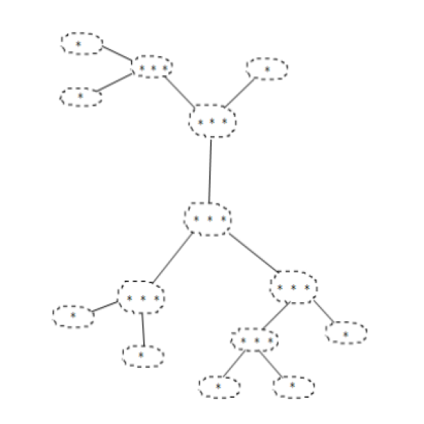
Figure 1. This GBT has 6 internal vertices, and 8 end vertices; all together, it involves $3\times 6+8=26$ group elements.

Definition 2.3.

A generalized binary tree $T$ of $F\subset\Gamma$ is called trivial if it has only 4 vertices, i.e. one root vertex and 3 end vertices. $T$ is called elementary if the level of every vertex is at most 3.

Definition 2.4.

If $T=(V,E)$ is a generalized binary tree of $F\subset\Gamma$, $A\subseteq V$, then the union of all subsets (triples or singletons) which represent the vertices of $A$ will be denoted by $S(A)$. In particular, the union of all subsets representing all vertices of $T$ will be denoted by $S(T)$.

Remark 2.5.

Notice that $S(A)\subseteq F$ for all $A\subseteq V$.

Definition 2.6.

The set of end vertices of a generalized binary tree $T=(V,E)$ will be denoted by $End(T)$, and the set of internal vertices will be denoted by $Int(T)$. Also, $Single(T),Central(T),Side(T)$ denote the set of all singleton vertices, central elements and side elements respectively.

Remark 2.7.

By the definition of a generalized binary tree, $Single(T)=End(T)$.

Definition 2.8.

For a generalized binary tree $T=(V,E)$, for all $v\in V\backslash\{root(T)\}$, $p(v)$ denotes the vertex which is adjacent to $v$ such that $level(p(v))=level(v)-1$; and for all $v\in V\backslash End(T)$, $n(v)$ denotes the set of vertices $v^{\prime}$ which are adjacent to $v$ such that $level(v^{\prime})=level(v)+1$.

Remark 2.9.

$n$ stands for next, $p$ stands for previous. If $v$ is an internal vertex then $n(v)$ consists of pair of vertices unless $v$ is a root.

We will need the following

Lemma 2.10.

If $T=(V,E)$ is a GBT then

$$|S(End(T))|\geq\frac{1}{4}|S(T)|$$

Proof.  The proof is by induction on $|S(T)|$.

For the trivial generalized binary tree we have $|S(T)|=6,|S(End(T)|=3$ so the inequality is satisfied. Let $T$ be any non-trivial GBT, and $v\in End(T),\ level(v)$ is maximal, $w=p(v)$. By definition, $v$ is a singleton and $w$ is a triple vertex.

Since $level(v)$ is maximal, $n(w)$ consists of pair of singleton vertices. Let $u$ denotes the other singleton vertex in $n(w)$. Let also $w=(a,b,c)$. We denote $w^{\prime}=(a)$.

By deleting $u$ and $v$ from $T$, and replacing $w$ with $w^{\prime}$ we obtain anew GBT $T^{\prime}$. Then $|S(T^{\prime})|=|S(T)|-4,|S(End(T^{\prime}))|=|S(End(T))|-1\ (\star)$. By inductive hypothesis, we have $|S(End(T^{\prime}))|\geq\frac{1}{4}|S(T^{\prime})|$ which, by $(\star)$, immediately implies $|S(End(T))|\geq\frac{1}{4}|S(T)|$  $\square$

Quasi-GBTs: We need even more general objects than GBTs, namely quasi-GBTs. A quasi-GBT is a somewhat degenerate form of a GBT. The major difference is that internal vertices of odd level are allowed to be pairs (instead of triples).

Definition 2.11.

A quasi-GBT $T=(V,E)$ of $F$ is a finite tree satisfying the following conditions:

(i) All vertices of $T$ have valence $i\in\{1,2,3\}$. Vertices of valence $i\in\{2,3\}$ are called internal vertices, and vertices of valence 1 are called end vertices.

(ii) All vertices of $T$ consist of $k$-tuples of elements of $F$ where $k\in\{1,2,3\}$. If a vertex has valence $i$ then it is an $i$-tuple. For two distinct vertices $u,v\in V$, their subsets, denoted by $S(u),S(v)$, are disjoint. The union of all subsets (triples, pairs or singletons) representing all vertices of $T$ will be denoted by $S(T)$

(iii) One of the vertices of $T$ is marked and called the root of $T$. The root is always an internal vertex, and contains three elements. We denote the root by $r(T)$.

(iv) For any finite ray $(a_{0}=r(T),a_{1},a_{2},\ldots,a_{k})$ of $T$ which starts at the root, and for any $i\in\{0,1,2,\ldots,k\}$ a vertex $a_{i}$ is called a a vertex of level $i$.

(v) A finite ray $(b_{0},b_{1},\ldots,b_{k})$ of $T$ is called level increasing if $level(b_{i})>level(b_{i-1})$ for all $1\leq i\leq k$.

(vi) One of the elements of each internal vertex is chosen and called a central element, the elements of the vertex other than central element are called side elements.

(vii) vertices of even level are triples.

(viii) If $u$ is a vertex of level $n\geq 2$ of $T$ of valence $i\in\{2,3\}$, and $v_{1},\ldots,v_{i-1}$ are the adjacent vertices of level $n+1$, then the set of all vertices which are closer to $v_{i}$ than to $u$ form a branch of $T$ beyond vertex $u$. $T$ has $(i-1)$ branches beyond the vertex $u$.

(ix) Similar to (vii), we define the branches beyond the root vertex.

Definition 2.12 ($\eta$-normal quasi-GBT).

Let $\Gamma$ be a finitely generated group satisfying condition $(A)$. A quasi-GBT $T$ of $F\subset\Gamma$ is called $\eta$-normal if for every vertex $v$ of $T$, $S(T)\subset xH$ for some $x\in\Gamma$.

Labeled quasi-GBTs: We will introduce a bit more structure on quasi-GBTs.

Let $\Gamma$ be a finitely generated group satisfying condition $(A)$, $F\subset\Gamma$ be a finite subset of $\Gamma,\ F_{0}\subseteq F$ is partitioned into 2-element subsets $\{x,y\}$ such that $y\in\{x\xi,x\xi^{-1}\}$. Thus every element in $F_{0}$ has a $\xi$-partner which we denote by $N_{\xi}(x)$ and since $\xi$ is fixed, we will drop it and denote by $N(x)$. By definition, $N(N(x))=x,\forall x\in F_{0}$.

Let $T=(V,E)$ be a quasi-GBT of $F_{0}$. Assume that $e\in E(T)$ is an edge connecting $v,w\in V(T)$ such that $level(w)=level(v)+1$. Assume also that the following conditions are satisfied:

(L1) there exists $a\in S(v),b\in S(w)$ such that $a=N(b)$.

(L2) if $w$ is an internal vertex then $b$ is the central element of $w$ and $a$ is a side element of $v$.

Then we label the edge $e$ by the element $a^{-1}b$. We also will denote $a=start(e),b=end(e)$.

Definition 2.13.

A quasi-GBT $T=(V,E)$ of $F_{0}\subset\Gamma$ is called labeled if every edge $e=(v,w)\in E$ with $p(w)=v$ satisfies conditions (L1) and (L2) and labeled as described above.

Now, let $r=(b_{1},b_{2},\ldots,b_{k})$ be a finite level increasing ray in $T$, i.e. $level(b_{i})=level(b_{i-1})+1),\ \forall i\in\{2,3,\ldots,k\}$. We will associate an element $L(r)\in\Gamma$ to $r$.

Let $e_{i}$ be the edge connecting $b_{i}$ to $b_{i+1},1\leq i\leq k-1$ and $a_{i}=start(e_{i}),b_{i}=end(e_{i}),1\leq i\leq k-1$. Since $T$ is labeled, all edges $e_{1},e_{2},\ldots,e_{k-1}$ are labeled by some elements $l(e_{1}),l(e_{2}),\ldots,l(e_{k-1})\in\Gamma$.

On the other hand, for each vertex $b_{i},2\leq i\leq k-1$ we assign $l(b_{i})=end(e_{i-1})^{-1}start(e_{i})$.

Thus all vertices $b_{2},b_{3},\ldots,b_{k-1}$ are labeled by some elements $l(b_{2}),l(b_{3}),\\ \ldots,l(b_{k-1})$. [However, notice that the labeling of these vertices actually depend on $r$; if $r,r^{\prime}$ are finite level increasing rays passing through the vertex $v$ and diverging at $v$ then the label of $v$ with respect to $r$ will differ from the label of $v$ with respect to $r^{\prime}$].

Then we associate the group element $l(e_{1})l(b_{2})l(e_{2})\ldots l(b_{k-1})l(e_{k-1})$ to $r$ which we will denote by $L(r)$.

Remark 2.14.

Notice that in a labeled quasi-GBT we associate a word $L(r)$ to every level increasing ray $r$. Notice also that the labeling structure of a generalized binary tree of $F$ depends on the choice of non-torsion element $\xi\in\Gamma$ and subset $F_{0}\subset F$ which can be partitioned into pairs of $\xi$-partners, and it depends on the partitioning as well.

At the end of this section, we would like to introduce an important structure on quasi-GBTs, namely, the order. This notion will be crucial, in the proof of Theorem 1.3 for guaranteeing that in building super-quasi-GBTs we do not get loops, so there is no obstacle in building the trees.

Definition 2.15 (Order).

Let $T$ be a super-quasi-GBT. Let $<$ be a linear order on the set of vertices $V(T)$ which satisfies the following conditions

(i) $root(T)<v$ for all $v\in V(T)\backslash\{root(T)\}$;

(ii) for all $u,v,w\in V(T)$ if $u<v$ and $w$ belongs to the branch beyond $v$ then $w<u$.

Then $T$ with $<$ will be called ordered.

Remark 2.16.

Notice that if $v$ is a vertex of level $n\geq 0$ of an ordered quasi-GBT $T$, and $v_{1},\ldots,v_{k}$ are all vertices of level $n+1$ adjacent to $v$ (i.e. $n(v)=\{v_{1},\ldots,v_{k})$, then we have a complete freedom in defining the order on $\{v_{1},\ldots,v_{k}\}$. However, notice that defining the order on the set $n(v)$ for each $v$ defines the order on the whole set $V(T)$

3. Zigzags and other intermediate notions

In this section we will assume that $\Gamma$ is a finitely generated group satisfying condition $(A)$. A good and useful example of such a group is the group $\mathbb{Z}^{2}$ itself.

Definition 3.1 (Zigzags, quasi-zigzags).

Let $H_{odd}=\{\eta^{2n+1}\ |n\in\mathbb{Z}\},\ H^{\prime}_{odd}=\{\xi^{2n+1}\ |n\in\mathbb{Z}\}$. For every $x\in\Gamma$, we call the sets $xH$ and $xH^{\prime}$ the horizontal lines and the vertical lines, respectively, passing through $x$.

A sequence $Z=(x_{1},x_{2},\ldots,x_{m})$ of elements of $\Gamma$ will be called a zigzag if for all $1\leq i\leq m-2$,   either $x_{i}^{-1}x_{i+1}\in H_{odd}$ or $x_{i}^{-1}x_{i+1}\in H^{\prime}_{odd}$; moreover, $x_{i}^{-1}x_{i+1}\in H_{odd}\Rightarrow x_{i+1}^{-1}x_{i+2}\in H^{\prime}_{odd}$ and $x_{i}^{-1}x_{i+1}\in H^{\prime}_{odd}\Rightarrow x_{i+1}^{-1}x_{i+2}\in H_{odd}$.

A sequence $Z=(x_{1},x_{2},\ldots,x_{m})$ of elements of $\Gamma$ will be called a quasi-zigzag if for all $1\leq i\leq m-2$,   either $x_{i}^{-1}x_{i+1}\in H$ or $x_{i}^{-1}x_{i+1}\in H^{\prime}_{odd}$; moreover, $x_{i}^{-1}x_{i+1}\in H\Rightarrow x_{i+1}^{-1}x_{i+2}\in H^{\prime}_{odd}$ and $x_{i}^{-1}x_{i+1}\in H^{\prime}_{odd}\Rightarrow x_{i+1}^{-1}x_{i+2}\in H$.

The number $m$ will be called the length of Z.

Notice that given any horizontal line $L$ and any zigzag $Z=(x_{1},x_{2},\ldots,x_{m})$ in $\Gamma$ with distinct elements, if $m\geq 3$ and $x_{1},x_{m}\notin L$ then we have $|Z\cap L|=2n,n\in\mathbb{N}\cup\{0\}$. We will need more structures on a zigzag

Definition 3.2 (balanced zigzags).

A (quasi-)zigzag $Z=(x_{1},x_{2},\ldots,x_{m})$ is called balanced if the following conditions are satisfied:

(i) for all $1\leq i\leq m-3$, and $\epsilon\in\{-1,1\}$, we have $x_{i}^{-1}x_{i+1}=\xi^{\epsilon p}\Rightarrow x_{i+2}^{-1}x_{i+3}\in\xi^{-\epsilon p}$.

(ii) either $x_{1}^{-1}x_{2}=\xi^{-p}$ or $x_{2}^{-1}x_{3}=\xi^{-p}$

Example: A zigzag

$Z=(z,z\eta^{n_{1}},z\eta^{n_{1}}\xi^{-p},z\eta^{n_{1}}\xi^{-p}\eta^{n_{2}},z\eta^{n_{1}}\xi^{-p}\eta^{n_{2}}\xi^{p},z\eta^{n_{1}}\xi^{-p}\eta^{n_{2}}\xi^{p}\eta^{n_{3}},\\ z\eta^{n_{1}}\xi^{-p}\eta^{n_{2}}\xi^{p}\eta^{n_{3}}\xi^{-p})$ is balanced, for all $n_{1},n_{2},n_{3}\in\mathbb{Z}_{odd}$.

Remark 3.3.

Notice that if a zigzag $Z=(x_{1},\ldots,x_{m})$ is balanced then the zigzag $Z^{-1}=(x_{m},\ldots,x_{1})$ is not necessarily balanced.

Definition 3.4.

Given subsets $A,B\subseteq\Gamma$, if there exists a balanced quasi-zigzag $Z=(x_{1},\ldots,x_{m})$ with $x_{1}\in A,x_{n}\in B$, then we say $B$ is connected to $A$ with a quasi-zigzag $Z$.

Balanced Segments. We will be working with tilings of the group $\Gamma$ into segments.

Definition 3.5 (Segments).

Let $x,y\in\Gamma$ belong to the same horizontal line $L$, and $x$ is on the left side of $y$, i.e. there exists $n\in\mathbb{N}$ such that $y=x\eta^{n}$. Then by $seg(x,y)$ we denote the finite set of all points (elements) in between $x$ and $y$ including $x$ and $y$, i.e. $seg(x,y)=\{x\eta^{i}\ |\ 0\leq i\leq n\}$. A finite subset $I$ of $L$ is called a segment if there exists $x,y\in I$ such that $I=seg(x,y)$.

Definition 3.6 (Balanced Segments).

A finite segment $I$ will be called a balanced segment if $|I|$ is divisible by 6.

Definition 3.7 (Leftmost and rightmost elements).

Let $I$ be a segment. Then there exists a unique element $z_{1}\in I$ such that for any $z\in I$ there exists a non-negative integer $n$ such that $z=z_{1}\eta^{n}$. The element $z_{1}$ will be called the leftmost element of $I$. Similarly, we define the rightmost element of $I$: there exists a unique element $z_{2}\in I$ such that for any $z\in I$ there exists a non-positive integer $n$ such that $z=z_{2}\eta^{n}$;  $z_{2}$ will be called the rightmost element of $I$

Definition 3.8 (Compatibility of zigzags and quasi-zigzags with tiling).

Let $\{I(x)\}_{x\in X}$ be a tiling of $\Gamma$ by balanced segments. A (quasi-)zigzag $Z=(x_{1},x_{2},\ldots x_{n})$ is called compatible with this tiling if for all $i\in\{1,\ldots,n-1\}$, if $x_{i},x_{i+1}$ lie on the same horizontal line then there exists $x\in X$ such that $x_{i},x_{i+1}\in I(x)$.

Definition 3.9 (Compatibility of GBT with tiling).

Let $\{I(x)\}_{x\in X}$ be a tiling of $\Gamma$ by balanced segments. A quasi-GBT $T$ of $\Gamma$ is called compatible with the tiling, if for all $v\in V(T)$, there exists $x\in X$ such that $S(v)\subset I(x)$.

We would like to conclude this section with introducing some notions for labeled $\eta$-normal generalized binary trees.

Definition 3.10 (starting element).

Let $T$ be a labeled $\eta$-normal quasi-GBT, and $a$ be the central element of $root(T)$. The element $N(a)$ will be called the starting element of $T$ and denoted by $start(T)$.

Definition 3.11 (special quasi-GBTs).

A labeled $\eta$-normal quasi-GBT is called special if $\{a^{\prime}\}$ is an end vertex where $a^{\prime}$ is the starting element of $T$.

In the proof of Theorem 1.3 the GBTs will be constructed piece-by-piece, in other words, some GBTs will be constructed as a union of elementary pieces. An trivial labeled $\eta$-normal GBT $T$ is called an elementary piece. If $T$ is special as a quasi-GBT then it is called a special elementary piece, otherwise we call it an ordinary elementary piece.

It is useful to observe that quasi-GBTs can be obtained from a GBT as follows: Let $T$ be an $\eta$-normal and labeled GBT. Let also $v_{1},\ldots,v_{k}\in Int(T)$ be not necessarily distinct internal vertices such that $v_{i}\neq root(T)$ for any $i\in\{1,\ldots,k\}$. Let $a_{i}\in S(v_{i}),1\leq i\leq k$, such that $level(N(a_{i}))=level(a_{i})+1$, $level(a_{i})\in\mathbb{Z}_{odd}$, and let $w_{i}\in V(T)$ be such that $N(a_{i})\in S(w_{i})$. Finally, let $S_{i}=\{v\in V(T)\ |\ v$ belongs to some level increasing ray $r$ which starts at $w_{i}\}$. By deleting $\displaystyle\mathop{\sqcup}_{1\leq i\leq k}\{a_{i}\}\sqcup S(S_{i})$ from $T$ we obtain an $\eta$-normal and labeled quasi-GBT. If $T$ is a special GBT then we obtain a special $\eta$-normal and labeled quasi-GBT.

Definition 3.12.

Let $T$ be a labeled $\eta$-normal quasi-GBT. We say $T$ is successful if it contains a triple vertex of odd level.

4. Generalized binary trees in partner assigned regions

In this section, we will be assuming that $\Gamma$ is a finitely generated group satisfying conditions $(A)$ and $(D)$, $K=B_{2000p}(1)\subset\Gamma$, $\epsilon=\frac{1}{100|K|}$, $F$ is a connected $(K,\epsilon)$-Følner set, $\{I(x)\}_{x\in X}$ be a collection of pairwise disjoint balanced segments of length at most 1200 tiling $\Gamma$. Let also $X_{0}=\{x\in X\ |\ I(x)\cap Int_{K}F\neq\emptyset\},F_{1}=\displaystyle\mathop{\cup}_{x\in X_{0}}I(x)$.

We will need the following notions

Definition 4.1 (Regions).

A subset $S\subseteq F_{1}$ is called a region if there exists $X_{0}^{\prime}\subset X$ such that $S=\displaystyle\mathop{\sqcup}_{x\in X_{0}^{\prime}}I(x)$. For any subset $S^{\prime}\subset F_{1}$ we will denote the minimal region containing $S^{\prime}$ by $R(S^{\prime})$.

Definition 4.2 (Partner assigned regions).

A region $S\subseteq F_{1}$ is called partner assigned if there exists a subset $S_{0}\subseteq S$ and a function $n:S_{0}\rightarrow\mathbb{Z}_{\textrm{odd}}$ such that

$$S\subseteq\displaystyle\mathop{\sqcup}_{x\in S_{0}}\{x,x\xi^{n(x)}\}\subseteq F$$

We will denote $x\xi^{n(x)}=N(x)$ and $x=N(x\xi^{n(x)})$. Also, for any subset $A\subseteq S$, we will write $N(A)=\{N(x)\ |\ x\in A\}$.

Notice that the partners of elements from $F_{1}$ do not necessarily lie in $F_{1}$ but they always lie in $F$. In the proof of Theorem 1.3 we will be assigning partners of elements of $F_{1}$ before we start building the trees, so $F_{1}$ will be a partner assigned region. We will arrange the partner assignment to satisfy certain conditions to enable us to push the rays of the trees to higher levels or at least not to let them come below certain level.

Definition 4.3 (Zigzags and GBTs respecting partner assignment).

Let $S\subseteq F_{1}$ be a partner assigned region and $Z=(x_{1},x_{2},\ldots,x_{n})$ be a quasi-zigzag in $S$. We say $Z$ respects partner assignment of $S$ if for all $i\in\{1,\ldots,n-1\}$, if $z_{i}$ and $z_{i+1}$ do not lie on the same horizontal line then $z_{i+1}=N(z_{i})$.

We say a quasi-GBT $T$ is respecting the given partner assignment if it is a labeled quasi-GBT with respect to this partner assignment.

A partner assignment induces labeling structure for a quasi-GBT $T$; from now on we will identify the notion of “labeled quasi-GBT” with the notion of a “quasi-GBT respecting the partner assignment”. We will also identify the notion of “balanced (quasi-)zigzag” with the notion of a “(quasi-)zigzag respecting the partner assignment”, if the partner assignment is fixed. (Notice that if a quasi-zigzag satisfies our fixed partner assignment, then it is balanced; cf. Definitions 3.1 and 3.2.)

Definition 4.4.

An element $z\in F_{1}$ is called successful if at least one of the following three conditions are satisfied:

(i) $h(z\xi^{-p})=h(z)+p$.

(ii) $N(z)\notin F_{1}$

(iii) $N(z)=z\xi^{p}$

Otherwise, $z$ is called unsuccessful.

More generally, for any region $S\subseteq F_{1}$, we say $z\in S$ is a successful element of $S$, if either at least one of conditions (i), (iii) are satisfied, or $N(z)\notin S$.

Now we will introduce a certain partner assignments for regions in $F_{1}$. First, we describe a certain natural tiling and partner assignment of the group $\mathbb{Z}^{2}$. Namely, for every $m,n\in\mathbb{Z}$, we let $I_{m,n}=\{(x,m)\in\mathbb{Z}^{2}\ |\ 360n\leq x<360(n+1)$. The partner assignment will be defined as follows: for every $(x,y)\in\mathbb{Z}$, $N(x,y)=(x,y+p)$ if $y$ is even, and $N(x,y)=(x,y-p)$ if $y$ is odd.

Remark 4.5.

In the group $\mathbb{Z}^{2}$ with standard generating set $\eta=(1,0),\xi=(1,0)$, let us assume the above tiling $\{I_{m,n}\}_{m,n\in\mathbb{Z}}$ and the partner assignment, and let $p=1,h(x,y)=|y|,\mathrm{for\ all}\ (x,y)\in\mathbb{Z}^{2}$. Then for every quasi-zigzag $Z$ in $\mathbb{Z}^{2}$ which starts at element $g\in\mathbb{Z}^{2}$, and respects the given partner assignment, we have $h(z)\in(h(g)-1,h(g),h(g)+1)$ for all $z\in Z$.

Remark 4.6.

The above tiling and partner assignment immediately induces the pull back tiling by balanced segments of length $360$ and partner assignment through the epimorphism $\pi:\Gamma\rightarrow\mathbb{Z}^{2}$ which satisfies the following conditions:

(i) for all $x\in\Gamma$ either $N(x)=x\xi^{p}$ or $N(x)=x\xi^{-p}$.

(ii) for all $\epsilon\in\{-1,1\}$, if $x,y\in\Gamma$ are on the same horizontal line and $N(x)=x\xi^{\epsilon p}$ then $N(y)=y\xi^{\epsilon p}$.

We will fix this tiling in $\Gamma$ and the partner assignment for the rest of the paper. Notice that any zigzag $Z=(x_{1},\ldots,x_{m})$ which respects this tiling and the partner assignment is necessarily balanced if $x_{1}^{-1}x_{2}=\xi^{-p}$ or $x_{2}^{-1}x_{3}=\xi^{-p}$.

We now would like to introduce more structures on the partner assigned regions as well as on quasi-GBTs in partner assigned regions.

Definition 4.7 (Suitable/unsuitable segments).

A segment $I(x),x\in X$ is called suitable if for some (consequently, for any) $g\in I(x)$ we have $\pi(g)=(x,y)\in\mathbb{Z}^{2}$ where $y\in\mathbb{Z}_{odd}$. If $I(x)$ is not suitable then it is called unsuitable.

Remark 4.8.

Notice that, by the definition of the partner assignment, the segment $I(x)$ is suitable iff for some (consequently, for any) $g\in I(x)$ we have $N(g)=g\xi^{-p}$.

Definition 4.9.

Let $T$ be an $\eta$-normal quasi-GBT, $v$ be a vertex of it, $J$ be a horizontal segment. We say $v$ belongs to $J$ if $S(v)\subseteq J$.

For the rest of the paper we make the following assumptions: let $\Gamma$ be a finitely generated amenable group satisfying conditions $(A)$ and $(D)$, $K=B_{2000p}(1)\subset\Gamma$, $\epsilon=\frac{1}{100|K|}$, $F$ be a connected $(K,\epsilon)$-Følner set, $\{I^{k}(x)\}_{x\in X,0\leq k\leq 359}$ be a tiling of $\Gamma$ by segments of length 3; and for all $x\in X$, let $I(x)$ be a balanced segment of length $360\times 3=1080$ such that $I(x)=\displaystyle\mathop{\sqcup}_{0\leq k\leq 359}I^{k}(x)$; we assume that the tiling $\{I(x)\}_{x\in X}$ is obtained by the pullback of the tiling in Remark 4.5. Let also $X_{0}=\{x\in X\ |\ I(x)\cap Int_{K}F\neq\emptyset\},F_{1}=\displaystyle\mathop{\cup}_{x\in X_{0}}I(x)$, and let $\overline{F_{1}}=F_{1}\cup N(F_{1})$. All the labeled $\eta$-normal GBTs and quasi-GBTs will respect this tiling $\{I(x)\}_{x\in X}$ and the fixed partner assignment, and all the elementary pieces will respect the tiling $\{I^{k}(x)\}_{x\in X,0\leq k\leq 359}$. The notion of the region will be understood with respect to this tiling, i.e. a subset $S\subseteq F_{1}$ will be called a region if there exists a subset $Y\subseteq X\times\{0,\ldots,359\}$ such that $S=\displaystyle\mathop{\sqcup}_{(x,k)\in Y}I^{k}(x)$.

For every $x\in X$, let $I(x)=\{z(x)\eta^{i}\ |\ 0\leq i\leq 1079\},z(x)\in\Gamma$. Then we let $I^{k}(x)=\{z(x)\eta^{i}\ |\ 3k\leq i<3k+3\},\ 0\leq k\leq 359,J^{l}(x)=\{z(x)\eta^{j}\ |\ 6l\leq j<6l+6\},\ 0\leq l\leq 179$. The intervals $I^{k}(x),0\leq k\leq 359$ will be called short intervals, and the intervals $J^{l}(x),0\leq l\leq 179$ will be called medium intervals. All the labeled $\eta$-normal quasi-GBTs will respect the tiling $\{I^{k}(x)\},0\leq l\leq 359,x\in X$ unless specifically stated otherwise in which case they will respect the tiling $\{J^{l}(x)\},0\leq l\leq 179,x\in X$.

We will say that a short segment $I^{k}(x),x\in X,0\leq k\leq 359$ is suitable (unsuitable) if the segment $I(x)$ is suitable (unsuitable). We will write $Y_{0}=\{(x,k)\ |\ x\in X_{0},0\leq k\leq 359\}$. We will assume that all the labeled GBTs and quasi-GBTs have a root consisting of a suitable short segment.

We may and will assume that there is no unsuitable segment $I^{k}(x)\subset F_{1}$ such that for some $z\in I^{k}(x)$, $N(z)\notin F_{1}$. Also, we will assume that $F_{1}$ has at least as many suitable medium intervals as non-suitable ones.

If $u,v$ are on the same horizontal line and $u=v\eta^{n},n\in\mathbb{Z}$, we will write $d(u,v)=|n|$. For $g\in\Gamma,\ |g|$ will denote the length of $g$ in the left invariant Cayley metric of $\Gamma$ w.r.t. the generating set $\{\xi,\eta\}$.

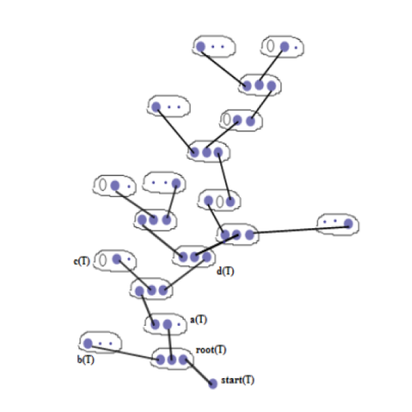
Figure 2. This is a special labeled quasi-GBT with a root vertex $\mathrm{root}(T)$, starting element $\mathrm{start}(T)$, and different types of vertices $a(T),b(t),c(T)$ and $d(T)$. A vertex is a $k$-tuple ($k\in\{1,2,3\}$) iff it contains $k$ big black dots; an empty circle indicates that the element is omitted, and the small dot means the element is not in $F_{1}$.

5. Completeness

We make the assumptions of Section 4.

In this section we introduce a key notion of completeness of quasi-GBTs. The completeness of the sequence $T_{1},T_{2},\ldots T_{m}$ simply means that we do not stop the trees unnecessarily.

Definition 5.1 (Complete sequence of quasi-GBTs.).

Let $T_{1},T_{2},\ldots,T_{n}$ be a sequence of mutually disjoint labeled $\eta$-normal quasi-GBTs of $F$. We say this sequence is pre-complete if for every $i\in\{1,\ldots,n\}$

(i) the root of $T_{i}$ consists of a triple $I^{k}(y)\subset F_{1},y\in X,0\leq k\leq 359$, where $I(y)$ is a suitable segment;

(ii) the singleton vertices (i.e. end vertices) of $T_{i}$ belong to unsuitable segments;

(iii) if $v$ is a vertex of even level of $T_{i}$ then $v$ is a triple and $S(v)=I^{l}(z)$ where $I^{l}(z)\subset F_{1},z\in X,0\leq l\leq 359$;

$T_{1},T_{2},\ldots,T_{n}$ is called complete if, in addition, for all $v=\{x\}\in Single(T_{i})$ with $x\in I^{k}(x_{0})\subseteq F_{1},x_{0}\in X,0\leq k\leq 359$, at least one of the following conditions hold

(i) there exists $j\in\{1,\ldots,i-1\}$ such that for some $w\in V(T_{j})$, $I^{k}(x_{0})\backslash\{x\}=S(w)$;

(ii) $T_{i}$ is a special quasi-GBT, $I(x_{0})$ is a non-suitable segment, and $x$ is a starting element of $T_{i}$;

(iii) there exists $j\in\{1,\ldots,i-1\},x^{\prime}\in I^{k}(x_{0})\backslash\{x\}$ such that $T_{j}$ is a special quasi-GBT and $x^{\prime}$ is the starting element of $T_{j}$.

Definition 5.2 (Successful complete sequence).

Let $T_{1},T_{2},\ldots,T_{n}(\ast)$ be a complete sequence of labeled $\eta$-normal quasi-GBTs of $F$ and $I$ be an unsuitable short segment in $F_{1}$. We say $(\ast)$ is successful at $I$ if one of the following conditions hold:

(i) there exist distinct $z_{1},z_{2}\in I$ such that $z_{1}=start(T_{i}),z_{2}=start(T_{j})$ for some $i,j\in\{1,\dots,n\}$.

ii) there exist $i,j\in\{1,\dots,n\}$ such that $start(T_{i})\sqcup S(v)=I$ where $v$ is a pair vertex of $T_{j}$.

iii) there exist $i\in\{1,\dots,n\}$ such that $S(v)=I$ for some triple vertex $v$ of $T_{i}$.

Notice that if a pre-complete sequence $T_{1},T_{2},\ldots,T_{n}$ satisfies the condition $\displaystyle\mathop{\sqcup}_{1\leq i\leq m}S(T_{i})\supseteq F_{1}$ then it is complete unless there exists an unsuitable segment $I=I^{k}(x)=\{z_{1},z_{2},z_{3}\}\subset F_{1}$ such that for all $i\in\{1,2,3\}$, there exists $j\in\{1,\dots,n\}$ such that $\{z_{i}\}$ is an end vertex of $T_{j}$, moreover, if $T_{j}$ is a special quasi-GBT, then $z_{i}$ is not a starting element of $T_{j}$. In this case, we will say that the sequence $(T_{1},\dots,T_{m})$ is unsuccessful at $I$.

It will be useful to observe that labeled quasi-GBTs can be obtained from a labeled GBTs by simply deleting some branches. Let $T$ be a labeled GBT such that all the internal vertices of $T$ are triples of the form $(z,z\eta^{n_{1}},z\eta^{n_{2}})$ for some $n_{1},n_{2}\in\mathbb{Z}$; moreover, all end vertices are of even level. Let $v_{1},\ldots,v_{k}\in Int(T)$ such that $level(v_{i})\in\mathbb{Z}_{odd}$ for all $1\leq i\leq k$. Let also $a_{i}\in S(v_{i}),1\leq i\leq k$ such that level $(N(a_{i}))=level(a_{i})+1$, and let $w_{i}\in V(T)$ be such that $N(a_{i})\in S(w_{i})$. Finally let $S_{i}=\{v\in V(T)\ |\ v\ \mathrm{belongs\ to\ some\ level}$   $\mathrm{increasing\ ray}\ r\ \mathrm{which\ starts\ at}\ w_{i}\}$. By deleting $\sqcup_{1\leq i\leq k}\{a_{i}\}\sqcup S(S_{i})$ from $T$ we obtain an ordinary labeled quasi-GBT $R$. If $T$ is special (or respects the partner assignment, or a tiling) then we will say that $R$ is special (or respects the partner assignment, or a tiling). Notice that the definition of labeled quasi-GBT as in the above construction agrees with the definitions 2.11 (quasi-GBT) and 2.13 (labeled quasi-GBT).

The following proposition will be very useful in the proof of Theorem 1.3.

Proposition 5.3.

Let $T_{1},T_{2},\ldots,T_{m}$ be a complete sequence of labeled $\eta$-normal quasi-GBTs of $F$ such that $\displaystyle\mathop{\sqcup}_{1\leq i\leq m}S(T_{i})\supset F_{1}$. Assume that for every ball $B_{20p}(g),g\in F_{1}$ there exists $i\in\{1,\ldots,m\}$ such that $T_{i}$ is successful and $S(T_{i})\cap B_{20p}(g)\neq\emptyset$. Then $|\partial_{K}F|\geq\frac{1}{100|B_{50p}|}|F|$. $\square$

Proof. Let us recall that for every $x\in X$, $I(x)=\{z(x)\eta^{i}\ |\ 0\leq i\leq 1079\}$, where $z(x)\in\Gamma$ is the leftmost element of $I(x)$, and $I^{k}(x)=\{z(x)\eta^{i}\ |\ 3k\leq i<3k+1\}$. We also have $J^{l}(x)=I^{2l}(x)\sqcup I^{2l+1}(x)$ for all $x\in X,0\leq l\leq 179$. Notice that $\{J^{l}(x)\}_{x\in X,0\leq l\leq 179}$ forms a tiling of $\Gamma$; also every $J^{l}(x)$ has length 6 and contains exactly two short intervals; we will call these short intervals neighbors.

Let $Z_{1}=\{2l+1\ |\ 0\leq l\leq 179\},Z_{2}=\{2l\ |\ 0\leq l\leq 179\},F_{1}^{-}=\sqcup_{x\in X_{0},k\in Z_{2}}I^{k}(x),F_{1}^{+}=\sqcup_{x\in X_{0},k\in Z_{1}}I^{k}(x)$. Notice that $F_{1}=F_{1}^{-}\sqcup F_{1}^{+}$. Notice also that, since the quasi-GBTs $T_{1},\ldots,T_{m}$ respect the tiling $\displaystyle\mathop{\sqcup}_{x\in X_{0},0\leq k\leq 359}I^{k}(x)$, for all $i\in\{1,\ldots,m\}$, either $S(T_{i})\cap F_{1}^{-}=\emptyset$ or $S(T_{i})\cap F_{1}^{-}=\emptyset$. We may assume that if $v\in V(T_{i}),1\leq i\leq m$, and $S(v)\backslash F_{1}\neq\emptyset$ then $v$ is an end vertex; moreover, $F_{1}$ contains at least as many suitable segments as non-suitable ones. We will also assume that $F_{1}^{-}$ contains at least as many unsuitable short intervals at which $T_{1},T_{2},\ldots,T_{m}$ successful as $F_{1}^{+}$ (and we will ignore the successfulness in $F_{1}^{+}$). We may furthermore assume that for some $1\leq m^{\prime}<m$, $S(T_{i})\cap F_{1}^{-}=\emptyset$ for all $1\leq i\leq m^{\prime}$, and $S(T_{i})\cap F_{1}^{+}=\emptyset$ for all $m^{\prime}+1\leq i\leq m$.

As agreed in Section 4, labeled $\eta$-normal quasi-GBTs $T_{1},\dots,T_{m}$ respect the tiling $\{I^{k}(x)\}_{x\in X,0\leq l\leq 359}$. Notice that for such a quasi-GBT $T$, if $I_{1},I_{2}$ are two neighboring short intervals, then for all $1\leq i\leq m$, either $S(T_{i})\cap I_{1}=\emptyset$ or $S(T_{i})\cap I_{2}=\emptyset$. In the proof below, we will construct labeled $\eta$-normal quasi-GBTs will respect just the tiling $\{J^{l}(x)\}_{x\in X,0\leq l\leq 179}$. Recall that by the agreement the root and more generally, all vertices of even level of any labeled $\eta$-normal quasi-GBT consists of a suitable short interval.

Let $J_{i}=I_{i}^{-}\sqcup I_{i}^{+},1\leq i\leq N$ be all medium intervals in $F_{1}$ such that $I_{i}^{-},I_{i}^{+}$ are the neighboring short intervals and at $I_{i}^{-}$ the sequence $T_{1},\ldots,T_{m}$ is successful. We will call the intervals $J_{i},1\leq i\leq N$ successful.

The main idea is to construct GBTs $\Omega=(\overline{T}_{1},\ldots,\overline{T}_{M})$ of $F$ such that the following conditions hold:

$(c1):$ every suitable short interval in $F_{1}$ forms an internal vertex of one of the GBTs from $\Omega$;

$(c2):$ every unsuitable medium interval in $F_{1}$ contains an internal vertex of one of the GBTs from $\Omega$;

$(c3)$ every successful medium interval contains either two internal vertices or one internal vertex and one starting element of GBTs from $\Omega$.

Let now $T$ be a labeled $\eta$-normal quasi-GBT and $R$ be a labeled quasi-GBT such that $S(R)\cap S(T)=\emptyset$. We introduce the following types of operations:

breaking up a quasi-GBT: Let $v$ be a pair vertex of $T,\ S(v)=\{a,b\},level(a)=level(N(a))+1,level(b)=level(N(b))-1$. Let also $w$ be a vertex of $T$ such that $N(b)\in S(w)$. Then $w$ is a triple vertex and is adjacent to two vertices $w_{1},w_{2}$. Let $V_{i}=\{v\in V(T)\ |\ v$ belongs to some level increasing ray $r$ which starts at $w_{i}\}$ for all $i\in\{1,2\}$. $S_{i}=\{v\in V(T)\ |\ v$ belongs to some level increasing ray $r$ which starts at $w_{i}\}$. Then $S:=\{b\}\sqcup S(w)\sqcup S(w_{1})\sqcup S(w_{2})\sqcup S(V_{1})\sqcup S(V_{2})$ forms a labeled $\eta$-normal quasi-GBT, while $S(T)\backslash S$ forms another labeled $\eta$-normal quasi-GBT. Hence, $T$ can be broken into two labeled $\eta$-normal quasi-GBTs. If we break $T$ at all of its $k$ pair vertices (notice that $k\leq 3$) then we obtain $k+1$ $\eta$-normal quasi-GBTs. We will call these $\eta$-normal quasi-GBTs obtained as a result of break up.

gluing of type 1: Let $v$ be as above, $R$ be special, $\sigma_{1}=\{c_{1}\}$ be its starting vertex such that $v$ and $\sigma_{1}$ belong either to the same or neighboring short intervals. Then $S(T)\sqcup S(R)$ forms a new labeled quasi-GBT $R^{\prime}$ where $root(R^{\prime})=root(T)$, and the pair vertex $v$ is replaced with a triple vertex.

gluing of type 2: Let $R$ be special, $\sigma_{1}=\{c_{1}\}$ be its starting vertex and $\sigma_{2}=\{c_{2}\}$ be the end vertex of $T$ such that $c_{1},c_{2}$ belong to the same short interval. Then the union $S(T)\sqcup S(R)$ forms a new labeled quasi-GBT $R^{\prime}$ such that $root(R^{\prime})=root(T)$.

collecting special quasi-GBTs: Let $R_{1},R_{2},R_{3}$ be disjoint special labeled quasi-GBTs, with starting elements $s_{1},s_{2},s_{3}$ respectively. Then the set $S(R_{1})\sqcup S(R_{2})\sqcup S(R_{3})$ forms a GBT $R^{\prime}$ with $root(R^{\prime})=(s_{1},s_{2},s_{3})$. All internal vertices of $R^{\prime}$ consists of a triple on some horizontal line except perhaps the root.

Now, we are ready to start the proof. Inductively, for any $i\in\{1,\ldots,m^{\prime}\}$ we will associate a finite set of labeled quasi-GBTs $C_{i}=(S^{(i)}_{1},\ldots,S^{(i)}_{n_{i}})$ to the collection $T_{1},\ldots,T_{i}$ as follows:

Base: We let $n_{1}=1,S^{(1)}_{1}=T_{1}$.

Step: Assume that, for some $i\in\{1,\ldots,m^{\prime}-1\}$, $C_{i}=\{S^{(i)}_{1},\ldots,S^{(i)}_{n_{i}}\}$ is the set of labeled quasi-GBTs associated to $T_{1},\ldots,T_{i}$ such that $\displaystyle\mathop{\sqcup}_{1\leq q\leq n_{i}}S(S^{(i)}_{q})=\displaystyle\mathop{\sqcup}_{1\leq q\leq i}S(T_{q})$.

Let $\Sigma=\{\sigma_{1},\ldots,\sigma_{k}\}$ be a maximal subset of $End(T_{i+1})$ such that the following two conditions are satisfied:

(i) if $1\leq q_{1}<q_{2}\leq k$ then $\sigma_{q_{1}}$ and $\sigma_{q_{2}}$ do not belong to the same short interval;

(ii) for all $q\in\{1,\ldots,k\}$, $\sigma_{q}$ belongs to $F_{1}$.

If $\Sigma=\emptyset$ then we let $C_{i+1}=C_{i}\sqcup T_{i+1}$. Otherwise, we have $\sigma_{1}:=\{c_{1}\}$ belongs to $F_{1}^{-}$. Let also $\sigma_{1}$ belongs to the short interval $I$. Then we have two cases:

Case 1: $I\backslash\displaystyle\mathop{\sqcup}_{1\leq q\leq n_{i}}S_{q}^{(i)}$ contains an element besides $c_{1}$.

Then, by completeness, we have two sub-cases:

a)  There exists $j\in\{1,\ldots,i\}$ such that the starting element $s$ of $T_{j}$ belong to the same short interval $I$ as $\sigma_{1}$.

Then we perform gluing of type 2, between $\sigma_{1}$ and $s$.

b)  $I\cap\displaystyle\mathop{\sqcup}_{1\leq q\leq n_{i}}S_{q}^{(i)}=\emptyset$ and $c_{1}$ is the starting element of $T_{i+1}$.

In this case we do not perform any operation and go to $\sigma_{2}$.

Case 2: $I\backslash\displaystyle\mathop{\sqcup}_{1\leq q\leq n_{i}}S_{q}^{(i)}$ contains no element besides $c_{1}$.

Then we do not perform any operation and by going to $\sigma_{2}$, apply the process to $\sigma_{2}$, and so on.

Once we are done with all the list $\{\sigma_{1},\ldots,\sigma_{k}\}$ we obtain a new set $C_{i+1}$. We denote the final collection $C_{m^{\prime}}=\{S^{(m^{\prime})}_{1},\ldots,S^{(m^{\prime})}_{n_{m^{\prime}}}\}$ by $D=\{S_{1},\ldots,S_{n}\}$.

Notice that as a result of the construction, the collection $D=\{S_{1},\ldots,S_{n}\}$ of labeled quasi-GBTs satisfies the following conditions:

(i) $S_{q_{1}}\cap S_{q_{2}}=\emptyset$, for all $1\leq q_{1}<q_{2}\leq n$;

(ii) $\displaystyle\mathop{\sqcup}_{1\leq q\leq n}S(S_{q})=\displaystyle\mathop{\sqcup}_{1\leq q\leq m^{\prime}}S(T_{q})$;

(iii) any short interval in $F_{1}^{-}$ contains either a pair vertex or a triple vertex of one of the quasi-GBTs from $D$, or it consists of three starting elements of some three quasi-GBTs from $D$;

Now, inductively on $j\in\{0,1,\ldots,m-m^{\prime}\}$, we associate a finite set of labeled quasi-GBTs $D_{j}=\{R^{(j)}_{1},\ldots,R^{(j)}_{k_{j}}\}$ to the collection $T_{m^{\prime}},T_{m^{\prime}+1},\ldots,T_{m^{\prime}+j}$ as follows:

Base: $D_{0}=D$.

Step: For $j\in\{1,\ldots,m-m^{\prime}\}$, we perform break up operations at all pair vertices of $T_{m^{\prime}+j}$, and let $\Phi_{1},\ldots,\Phi_{r}$ be a set of all quasi-GBTs and $\Psi=\{s_{1},\ldots,s_{r}\}$ be the set of starting elements obtained as a result of the break up. Let also $K_{0}\subseteq\{1,\ldots,r\}$ be the unique maximal subset such that for all $t\in K_{0}$ if $s_{t}$ belongs to the short interval $I$ then $I\cap\displaystyle\mathop{\sqcup}_{1\leq q\leq k_{j-1}}S(R^{(j-1)}_{q})=\emptyset$.

For all $t\in K_{0}$, let $s_{t}$ belongs to the short interval $I_{t}$ (recall that $I_{t}\subset F_{1}^{+}$). Let $I_{t}^{\prime}$ be the neighboring short interval in $F_{1}^{-}$.

Then we have one of the following two cases:

Case 1: $I_{t}^{\prime}$ contains a pair vertex of some labeled quasi-GBT $S$ from $D=D_{0}$.

Then we perform gluing of type 1 between $S$ and $\Phi_{t}$.

Case 2: $I_{t}^{\prime}$ contains a triple vertex of some labeled quasi-GBT $S$ from $D=D_{0}$.

Then we do not perform any operation and let $\Phi_{t}$ be one of the quasi-GBTs in the collection $R_{j}$ (so some of the quasi-GBTs $(\Phi_{t})_{t\in K_{0}}$ gets glued to one of the earlier quasi-GBTs from $D_{0}$ and some remain intact).

Then, on the final collection $D_{m-m^{\prime}}=\{R^{(m-m^{\prime})}_{1},\ldots,R^{(m-m^{\prime})}_{k_{m-m^{\prime}}}\}$, we perform the following operation: if any short interval $I\subset F_{1}^{-}$ consists of three starting elements of some three labeled quasi-GBTs then we collect these labeled quasi-GBTs into one GBT. We denote the resulting collection of GBTs by $\bar{D}$. Notice that, conditions (c1)-(c3) are satisfied for $\bar{D}$, i.e.:

(i) every suitable short interval in $F_{1}$ forms an internal vertex of one of the GBT from $\bar{D}$;

(ii) every unsuitable medium interval in $F_{1}$ contains an internal vertex of one of the GBT from $\bar{D}$;

(iii) every successful medium interval contains either two internal vertices or one internal vertex and one starting element of GBTs from $\bar{D}$.

Finally, we perform the following final operations on $\bar{D}$: if $\bar{D}$ contains $z=3z_{1}+z_{2}$ GBTs ($z_{1},z_{2}\in\mathbb{Z},z_{1}\geq 1,0\leq z_{2}\leq 2$) $\Xi_{1},\ldots,\Xi_{z}$ with starting elements in $F_{1}$ then for all $q\in\{0,\ldots,z_{1}-1\}$ we collect $\Xi_{3q+1},\Xi_{3q+2},\Xi_{3q+2}$ into a new GBT.

Let $R_{1},\ldots,R_{n}$ denotes the set of GBTs obtained as a result of the process. Then the following conditions hold:

(i) for every suitable medium interval $J\subseteq F_{1}$, $J\subset\displaystyle\mathop{\sqcup}_{1\leq i\leq n}S(Int(R_{i}))$;

(ii) for every unsuitable medium interval $J\subseteq F_{1}$, $|J\cap\displaystyle\mathop{\sqcup}_{1\leq i\leq n}S(Int(R_{i}))|\geq 3$;

(iii) for every successful unsuitable medium interval $J\subseteq F_{1}$, $|J\cap\displaystyle\mathop{\sqcup}_{1\leq i\leq n}S(Int(R_{i}))|\geq 4$.

Then, $|F_{1}\cap\displaystyle\mathop{\sqcup}_{1\leq i\leq n}S(End(R_{i}))|\leq\frac{1}{4}|F_{1}|(\ast)$, moreover, since the number of suitable medium intervals is not less than the number of unsuitable ones, we obtain that $|F_{1}\cap\sqcup_{1\leq i\leq n}S(Int(R_{i}))|\geq\frac{3}{4}|F_{1}|+\frac{1}{3}L$ where $L$ denotes the number of successful medium intervals.

Let $\Omega$ be a maximal subset of $F_{1}$ such that for any two distinct $x,y\in\Omega$, $d(x,y)\geq 70p$. Then $B_{35p}(x)\cap B_{35p}(y)=\emptyset$, moreover, $F_{1}\subseteq\cup_{x\in\Omega}B_{70p}(x)$. Then $|\Omega|\geq\frac{|F_{1}|}{|B_{70p}|}$.

Now, by the assumption every ball of radius $20p$ centered at $F_{1}$ has a non-empty intersection with a successful medium interval. Then every ball of radius $35p$ centered at $F_{1}$ (in particular, the balls $B_{35p}(x),x\in\Omega)$ contains a successful medium interval, thus we obtain that $L\geq|\Omega|\geq\frac{|F_{1}|}{|B_{70p}|}$.

Then, by Lemma 2.10 we obtain that

$$|\sqcup_{1\leq i\leq n}S(End(R_{i}))|\geq\frac{1}{3}(\frac{3}{4}|F_{1}|+\frac{1}{3}L)\geq\frac{1}{4}|F_{1}|+\frac{1}{9}L$$

Then, by $(\ast)$, $|\sqcup_{1\leq i\leq n}S(End(R_{i}))\backslash F_{1}|\geq\frac{1}{9}L\geq\frac{|F_{1}|}{9|B_{70p}|}$. Hence $|\partial_{K}F|\geq\frac{|F_{1}|}{9|B_{70p}|}$  $\square$

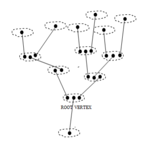
Figure 3. this labeled quasi-GBT has only one pair vertex.

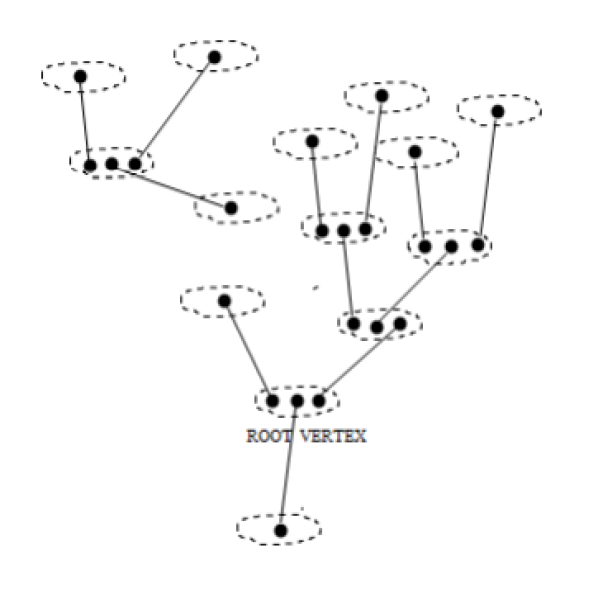
Figure 4. after the break up at the pair vertex, we obtain two new labeled quasi-GBT; one of them is a trivial GBT.

The following proposition follows immediately from the proof of Proposition 5.3

Proposition 5.4.

Let $T_{1},T_{2},\ldots,T_{m}(\ast)$ be a complete sequence of quasi-GBTs of $F$ such that $\displaystyle\mathop{\sqcup}_{1\leq i\leq m}S(T_{i})\supset F_{1}$. Assume that there exist $m+n$ short unsuitable intervals $I_{1},\ldots,I_{m},I_{m+1},\dots,I_{m+n}$ in $F_{1}$ such that $(\ast)$ is successful at $I_{j}$ for all $j\in\{1,\ldots,m\}$ and unsuccessful at $I_{j}$ for all $j\in\{m+1,\ldots,m+n\}$, moreover, $(\ast)$ is not unsuccessful at all other short unsuitable intervals of $F_{1}$. If $m-n\geq\frac{1}{100|B_{50p}|}|F|$, then $|\partial_{K}F|\geq\frac{1}{900|B_{50p}|}|F|$.  $\square$

6. The Proof of Theorem 1.3.

We make the assumptions of Section 4. The following notions will be needed

Definition 6.1.

Let $x_{1},x_{2}\in X,A_{1}\subseteq I(x_{1}),A_{2}\subseteq I(x_{2})$. We say $A_{1},A_{2}$ are connected by a quasi-zigzag if for some $u_{1}\in A_{1},u_{2}\in A_{2}$ there exists a quasi-zigzag $Z$ such that $Z$ starts at $u_{1}$ and ends at $u_{2}$. If $Z$ is also balanced, then we say $A_{2}$ is connected to $A_{1}$ by a balanced quasi-zigzag.

Definition 6.2.

Let $(x_{1},k_{1}),(x_{2},k_{2}),(x_{3},k_{3}),(x_{4},k_{4})\in Y_{0}$ and $I_{i}=I^{k_{i}}(x_{i}),1\leq i\leq 4$. We say the pairs $(I_{1},I_{2})$ and $(I_{3},I_{4})$ are connected with non-interfering zigzags if there exist zigzags $Z_{1},Z_{2}$ in $F_{1}$ such that $I_{1}$ and $I_{2}$ are connected by $Z_{1}$, $I_{3}$ and $I_{2}$ are connected by $Z_{2}$, moreover, there exists no $(x,k)\in Y_{0}$ such that $Z_{i}\cap I^{k}(x)\neq\emptyset$ for all $i\in\{1,2\}$.

We will also need the following notions

Definition 6.3.

Let $S\subseteq F_{1}$. We write $X(S)=\{(x,k)\in X_{0}\times\{0,\ldots,359\}\ |\ I^{k}(x)\subset S,I(x)\mathrm{\ is\ suitable}\},P(S)=\displaystyle\mathop{\sqcup}_{(x,k)\in X(S)}I^{k}(x)$.

Definition 6.4 (Extremal regions).

Let $g_{1},g_{2},\ldots,g_{n}\in\Gamma$ be distinct elements. Let the sub-region $S\subseteq F_{1}$ be such that there exist a sequence $(S_{0},S_{1},\ldots,S_{n})$ of subsets and sequences $(h_{1},\ldots,h_{n})$ and $(q_{1},\ldots,q_{n})$ of non-negative integers such that

(i) $S_{0}=P(F_{1})$;

(ii) $h_{i}=max\{h_{g_{i}}(z)\ |\ z\in S_{i-1}\}$, for all $1\leq i\leq n$;

(iii) $S_{i}=\{z\in S_{i-1}\ |\ h_{g_{i}}(z)\geq h_{i}-q_{i}\}$, for all $1\leq i\leq n$,

(iv) $S=S_{n}$.

We will write $R(g_{1},\ldots g_{n};q_{1},\ldots,q_{n})=S\cup N(S)\cup(\overline{F_{1}}\backslash F_{1})$, and call $R(g_{1},\ldots g_{n};q_{1},\ldots,q_{n})$ the extremal region of the sequence $(g_{1},\ldots,g_{n})$.

Remark 6.5.

In the above definition, $S_{n}$ are defined inductively. Notice that the set $S_{n}\cup N(S_{n})$ may contain a large region even if $q_{1}=q_{2}=\dots=q_{n}=0$. In general, since $h_{1},\dots,h_{n}$ are arbitrary non-negative integers, by taking them sufficiently big we also obtain that the entire $F_{1}$ (more precisely, $F_{1}\cup N(F_{1})\cup(\overline{F_{1}}\backslash F_{1})=F_{1}\cup(\overline{F_{1}}\backslash F_{1})$) is an extremal region. This observation will be used in the sequel, but the most interesting case of an extremal region is when $(q_{1},\ldots,q_{n})=(0,\ldots,0)$; this observation will be crucial in our study. A somewhat more general case of $0\leq q_{i}\leq 2p$, for all $1\leq i\leq n$ is also interesting but we will not be using it in this paper. Notice also that $S_{n}$ is a union of suitable segments. Moreover, although $S_{n}$ is a region, $R(g_{1},\ldots g_{n};q_{1},\ldots,q_{n})$ may not be; we hope this (calling it an extremal region) will not cause a confusion.

Remark 6.6.

We will sometimes denote the extremal region by $R(g_{1},\ldots,g_{n})$ dropping the sequence $(q_{1},\ldots,q_{n})$. Also, if $(q_{1},\ldots,q_{n})=(0,\ldots,0)$ then we will denote the extremal region by $R_{0}(g_{1},\ldots,g_{n})$.

The set $R(g_{1},\ldots,g_{n})$ heavily depends on the order of the sequence; for example, in general, $R(g_{1},g_{2})\neq R(g_{2},g_{1})$; in fact, it is quite possible that $R(g_{1},g_{2})\cap R(g_{2},g_{1})\subseteq\bar{F_{1}}\backslash F_{1}$.

Definition 6.7 (Minimal elements).

Let $I(x),x\in X$ be a suitable segment in the extremal region $R(g_{1},\ldots g_{n})$, and $I\subseteq I(x)$ be a sub-segment. We say $z\in I$ is a minimal element of $I$ if $z$ is unsuccessful with respect to some $h_{g_{i}},1\leq i\leq n$, and there is no $u\in I$ and $j\in\{1,\ldots,i-1\}$ such that $u$ is unsuccessful with respect to $h_{g_{j}}$. We say $z$ is an absolutely minimal element of $I$, if it is minimal, and for every other minimal $u\in I$,

$\mathrm{min}\{j:z\ \mathrm{is\ unsuccessful\ w.r.t.}\ h_{g_{j}},\ \mathrm{but}\ u\ \mathrm{is\ successful\ w.r.t.}\ h_{g_{j}}\}<\mathrm{min}\{j:u\ \mathrm{is\ unsuccessful\ w.r.t.}\ h_{g_{j}},\ \mathrm{but}\ z\ \mathrm{is\ successful\ w.r.t.}\ h_{g_{j}}\}$

Condition (i) of $(D)$ states that on a given horizontal segment of length 2 at most one element is unsuccessful with respect to the same $h_{g}$ . Then condition (ii) states that given an unsuccessful element $u$, one can relate to it an element $u^{\prime}$ in a certain special way such that not only $u^{\prime}$ is successful but even nicer property holds for $u^{\prime}$, namely, $h(u^{\prime}\xi^{-p}\eta^{i_{1}}\xi^{p}\eta^{i_{2}}\xi^{-p}\eta^{i_{3}}\xi^{p})=h(u^{\prime})+4p$ for certain values of $i_{1},i_{2},i_{3}$. Thus existence of an unsuccessful element $u$ is compensated by the existence of $u^{\prime}$ which is related to $u$ and is even better than successful.

We will materialize this idea in the proof. First, we need the following notions

Definition 6.8 (Successfully related elements).

Let $u\in I^{k}(x)\subset F_{1}$ be a suitable short interval, and $u\in I^{k}(x)$. We say an element $u^{\prime}$ is successfully related to $u$ if either $u^{\prime}=u\eta^{-i}\xi^{-p}\eta^{j}$, where $i\in\{1,2\},j\in[1,i],u\eta^{-i}\in I^{k}(x)$ or $u^{\prime}=u\eta^{i}\xi^{-p}\eta^{-j}$, where $i\in\{1,2\},j\in[1,i],u\eta^{i}\in I^{k}(x)$.

Definition 6.9 (Successfully related special elementary pieces).

Let $(g_{1},\ldots,g_{N})$ be a finite sequence of elements of $\Gamma$, and $u\in I=I^{k}(x)\subset F_{1},x\in X_{0},0\leq k\leq 359$, be such that $u$ is an absolutely minimal element of $I$. Let $T$ a labeled $\eta$-normal special elementary piece of $F$. We say $T$ is successfully related to $u$ if $N(u)$ is a starting element of $T$ (so, in particular, it is an end vertex). In this case we also say $T$ is successfully related to $I$.

Definition 6.10.

Let $T$ be a special elementary piece successfully related to $u\in I$ for some suitable short segment $I=I^{k}(x)=\{u,u_{1},u_{2}\},x\in X_{0},0\leq k\leq 359$. Let $A\subseteq F$. We say $T$ is successful relative to $A$, if for all $i\in\{1,2\}$, if $N(u_{i})$ belongs to an unsuitable short segment $I_{i}\subset F_{1}$, then $A$ contains all elements of $I_{i}$ which are successfully related to $u$.

Let us emphasize that if a suitable short segment $I=I^{k}(x)=\{z_{1},z_{2},z_{3}\}\subset F_{1}$, where $z_{1}$ and $z_{3}$ are the leftmost and rightmost elements of $I$ respectively, in the extremal region $R(g_{1},\ldots,g_{N})$ admits a minimal element but not an absolutely minimal element, then $I$ has exactly two minimal elements, namely, $z_{1}$ and $z_{3}$. Let $T$ be an ordinary elementary piece such that $root(T)=I$; we will denote the vertex of $T$ which contains $N(z_{i})$ by $v_{i},1\leq i\leq 3$. Let also $S(v_{i})\subseteq I_{i}=I^{k_{i}}(y_{i}),1\leq i\leq 3$.

Then both elements of $I_{2}\backslash S(v_{2})$ are successfully related to either $z_{1}$ or $z_{2}$; $N(z_{1})\eta$ is successfully related to $z_{3}$ and $N(z_{3})\eta^{-1}$ is successfully related to $z_{1}$. These observations are useful but in the sequel we will choose the sequence $(g_{1},\dots,g_{n})$ dense enough that every suitable short segment will contain an absolutely minimal element.

Now, we would like to introduce a notion of partial (or linear) order in the set of suitable short intervals of $F_{1}$ as well as in the set of all elements belonging to the suitable short intervals of $F_{1}$. The proof of Theorem 1.3 is based in constructing a complete sequence of elementary pieces or quasi-GBTs, and the order we introduce will indicate where to start the next quasi-GBT in the sequence at every step.

Partial Order: We now introduce a strict partial order in extremal regions [we say a relation $\sim$ on a set $S$ is a strict partial order if it is anti-symmetric, transitive, and there is no $x\in S$ such that $x\sim x$]. By prolonging the sequence of origins, this partial order can be made a linear order.

Let $R=R(g_{1},\ldots g_{n};q_{1},\ldots,q_{n})$ be an extremal region, and
$S(g_{1},\ldots g_{n};q_{1},\ldots,q_{n})$ be the set of all elements of $R(g_{1},\ldots g_{n};q_{1},\ldots,q_{n})$ which belong to suitable segments. Let also $Y_{R}=\{(x,k)\ |\ I^{k}(x)\subset S(g_{1},\ldots g_{n};q_{1},\ldots,q_{n})$. We will introduce a partial order $\prec$ on the set $Y_{R}$ and on the set $S(g_{1},\ldots g_{n};q_{1},\ldots,q_{n})$ as follows:

Let $y_{1},y_{2}\in Y_{R},y_{1}=(x_{1},k_{1}),y_{2}=(x_{2},k_{2})$. Let also $u_{i}\in I^{k_{i}}(x_{i}),1\leq i\leq 2$. We say $y_{2}\prec y_{1}$ if one of the following two conditions hold:

(c1) $\mathrm{min}\{i\in\{1,\ldots,n\}\ |\ h_{g_{i}}(u_{1})>h_{g_{i}}(u_{2})\}\leq\mathrm{min}\{i\in\{1,\ldots,n\}\ |\ h_{g_{i}}(u_{2})>h_{g_{i}}(u_{1})\}$, moreover, there exists $i\in\{1,\ldots,n\}$ such that $h_{g_{i}}(u_{1})\neq h_{g_{i}}(u_{2})$;

(c2) $h_{g_{i}}(u_{1})=h_{g_{i}}(u_{2})$ for all $i\in\{1,\ldots,n\}$, but

$\mathrm{min}\{i\in\{1,\ldots,n\}\ |\ I^{k_{1}}(x_{1})\ \mathrm{contains\ an\ unsuccessful\ element\ w.r.t.}\ h_{g_{i}}\}<\mathrm{min}\{i\in\{1,\ldots,n\}\ |\ I^{k_{2}}(x_{2})\ \mathrm{contains\ an\ unsuccessful\ element\ w.r.t.}\ h_{g_{i}}\}$ (so, in particular, there exists $i\in\{1,\ldots,n\}$ such that $I^{k_{1}}(x_{1})$ contains an unsuccessful element w.r.t. $h_{g_{i}}$).

Notice that, since the functions $h_{g}:\Gamma\rightarrow\mathbb{N}\cup\{0\}$ are constant on the horizontal lines, the definition does not depend on the choices $u_{1},u_{2}$. If $y_{2}\prec y_{1}$ then we also say $I^{k_{1}}(y_{1})$ is bigger than $I^{k_{2}}(y_{2})$. We also say $I^{k_{1}}(y_{1})$ is strongly bigger than $I^{k_{2}}(y_{2})$ if condition (c1) holds.

Let now $u,v\in S(g_{1},\ldots g_{n};q_{1},\ldots,q_{n}),u\in I^{k^{\prime}}(x^{\prime}),v\in I^{k^{\prime\prime}}(x^{\prime\prime}),y^{\prime}=(x^{\prime},k^{\prime}),y^{\prime\prime}=(x^{\prime\prime},k^{\prime\prime})$. If $y^{\prime}\prec y^{\prime\prime}$ then we let $u\prec v$. If $y^{\prime}\nprec y^{\prime\prime}$ and $y^{\prime\prime}\nprec y^{\prime}$ (in particular, if $y^{\prime}=y^{\prime\prime}$), we say $u\prec v$, if
$\mathrm{min}\{i\in\{1,\ldots,n\}\ |\ u\ \mathrm{is\ unsuccessful\ w.r.t.}\ h_{g_{i}}\mathrm{but}\ v\ \mathrm{is\ successful\ w.r.t.}\ h_{g_{i}}\}>\\ \mathrm{min}\{i\in\{1,\ldots,n\}\ |\ v\ \mathrm{is\ unsuccessful\ w.r.t.}\ h_{g_{i}}\ \mathrm{but}\ u\ \mathrm{is\ successful\ w.r.t.}\ h_{g_{i}}\}$.

Once we define the order $\prec$ on the set of suitable short segments of an extremal region (and on the set of elements which belong to suitable short segments of the extremal region) we can restrict it to any subset. Then it is clear from the condition D-(iii) that for any region $R\subseteq F_{1}$ (in particular, for the region $F_{1}$ itself) we can choose long enough sequence $g_{1},\ldots,g_{L}$ of origins such that for the choice $(q_{1},\ldots,q_{L})=(0,\ldots,0)$ the partial order $\prec$ on the set of suitable short segments of $R$ (and on the set elements which belong to suitable short segment of $R$) becomes a linear order. Indeed, in defining the partial order $\prec$, we observe that

$$R_{0}(g_{1})\supseteq R_{0}(g_{1},g_{2})\supseteq\dots\supseteq R_{0}(g_{1},g_{2},\dots,g_{L}).$$

Notice that $R_{0}(g_{1},g_{2},\dots,g_{L})$ is never empty. If it contains only one suitable short segment of $F_{1}$ then this segment is the biggest in our order. But if it contains more than one such segment then we look into the question of which one of them contains unsuccessful elements with respect to $h_{g_{i}}$ for the least possible $i$. This way of viewing our definition of the partial order motivates more general notion of extremal regions with constraints. We will avoid defining this notion in its most general natural version, but rather restrict ourselves to a certain type (two types) which will be used in the sequel.

First, we need a the following

Definition 6.11.

Let $Z=(x_{1},\dots,x_{n})$ be a zigzag in $F_{1}$ which respects the fixed tiling and partner assignment. We say $Z$ belongs to the class $\mathcal{R}_{left}$ ($\mathcal{R}_{right}$) if $x_{i}$ is not the leftmost (rightmost) element of any unsuitable short segment for all $1\leq i\leq n-1$ such that $x_{i}^{-1}x_{i+1}=\xi^{p}$.

Definition 6.12 (Extremal regions with constraints on the left).

Let $g_{1},g_{2},\ldots,g_{n}\in\Gamma$ be distinct elements and $I_{1},I_{2},\dots,I_{n}$ be a sequence of suitable short segments of $F_{1}$. Let the sub-region $S\subseteq F_{1}$ be such that there exist a sequence $(S_{0},S_{1},\ldots,S_{n})$ of subsets and sequences $(h_{1},\ldots,h_{n})$ and $(q_{1},\ldots,q_{n})$ of non-negative integers such that

(i) $S_{0}=P(F_{1})$;

(ii) $h_{i}=max\{h_{g_{i}}(z)\ |\ z\in S_{i-1}\}$, for all $1\leq i\leq n$;

(iii) for all $1\leq i\leq n$, $I_{i}\subseteq\{z\in S_{i-1}\ |\ h_{g_{i}}(z)\geq h_{i}-q_{i}\}$,

(iv) $S_{i}=\{z\in S_{i-1}\ |\ h_{g_{i}}(z)\geq h_{i}-q_{i},z\ \mathrm{is\ connected\ to}\ I_{i}\ \mathrm{by\ a\ zigzag\ from}\ \mathcal{R}_{left}\}$, for all $1\leq i\leq n$,

(v) $S=S_{n}$.

We will write $R(g_{1},\ldots g_{n};q_{1},\ldots,q_{n};I_{1},\dots,I_{n})=S\cup N(S)\cup(\overline{F_{1}}\backslash F_{1})$, and call $R(g_{1},\ldots g_{n};q_{1},\ldots,q_{n};I_{1},\dots,I_{n})$ the extremal region of the sequence $(g_{1},\ldots,g_{n})$.

By replacing conditions (iv) with following condition, we obtain the notion an extremal region with constraints on the right.

(iv)${}^{\prime}\ S_{i}=\{z\in S_{i-1}\ |\ h_{g_{i}}(z)\geq h_{i}-q_{i},z\ \mathrm{is\ connected\ to}\ I_{i}\ \mathrm{by\ a\ zigzag\ from}\ \mathcal{R}_{right}\}$, for all $1\leq i\leq n$,

Notice that conditions (i)-(v) imply that for all $1\leq i\leq n-1$, $I_{i+1}$ is connected to $I_{i}$ with a zigzag from $\mathcal{R}_{left}\}$.

In the definition of partial order above, by replacing $R(g_{1},\ldots g_{n};q_{1},\ldots,q_{n})$ with $R(g_{1},\ldots g_{n};q_{1},\ldots,q_{n};I_{1},\dots,I_{n})$ everywhere we define a partial order with constraint on the left (right). We will use partial orders both with and without constraints. Unless said otherwise “a partial order” will have no constraint.

We now fix the sequence $(g_{1},\ldots,g_{L})$ and study suitable short segments with respect to the order $\prec$ that it defines:

Definition 6.13.

Let $I=I^{k}(x)=\{u,v,w\}\subset F_{1}$ be a suitable short segment where $u$ is the leftmost and $w$ is the rightmost element; and let $\prec$ be a linear order on $P(F_{1})$. We will say $I$ is of

type 1, if $v\prec u$ and $v\prec w$;

type 2, if $u\prec v$ and $w\prec v$;

type 3, if $u\prec v\prec w$;

type 4, if $w\prec v\prec u$.

If $T$ is an elementary piece with root at $I=I^{k}(x)$, we say $T$ is of type 1 (or type 2, 3, 4), if $I$ is of type 1 (or type 2, 3, 4 respectively).

We also need the following notions

Definition 6.14 (exceptional regions).

Let $I=\{u_{1},\ldots,u_{m}\}\subseteq I(x)\subset P(F_{1})$ where elements of the segment are listed from leftmost to rightmost. We say $I$ is positively exceptional if $u_{1}\prec u_{2}\prec\ldots\prec u_{m}$; and negatively exceptional if $u_{m}\prec u_{m-1}\prec\ldots\prec u_{1}$; we say $I$ is exceptional if it is either positively or negatively exceptional. Similarly, we say a region $R\subseteq F_{1}$ is exceptional, if either all segments $I\subseteq P(R)$ are positively exceptional or they are all negatively exceptional.

Definition 6.15 (neighbor segments).

Let $I^{k^{\prime}}(x^{\prime}),I^{k^{\prime\prime}}(x^{\prime\prime})$ be suitable short segments in $F_{1}$. We say they are neighbors if there exists an unsuitable segment $I^{k}(x)\subseteq F_{1}$ and $u,v\in I^{k}(x)$ such that $u\xi^{p}\in I^{k^{\prime}}(x^{\prime}),v\xi^{p}\in I^{k^{\prime\prime}}(x^{\prime\prime})$. $I^{k}(x)$ will be called a connecting segment.

Remark 6.16.

In other words, two short intervals are neighbors if there is a quasi-zigzag of length 4 connecting them. Notice that by condition $D$-(iii) the connecting segment is unique.

Definition 6.17 (connected components).

A sub-region of $F_{1}$ is called connected if any two suitable short segments in it are connected with a quasi-zigzag respecting the tiling $\{I^{k}(x)\}_{x\in X,0\leq k\leq 359}$. If $R$ is a maximal connected sub-region of $F_{1}$ then $R\sqcup N(R)$ is called a connected component of $F_{1}$.

Now we are ready to start the proof of the theorem. Without loss of generality we may and will assume that $F_{1}$ is connected (otherwise we consider each connected component separately). Then, by Remark 2.3 if $u,v\in F_{1}$ belong to the suitable intervals of $F_{1}$ then either both $h(u),h(v)$ are even or both are odd; without loss of generality again we may and will assume that $h(u)$ is even whenever $u$ belongs to a suitable segment of $F_{1}$.

We can choose a sequence $g_{1},\ldots,g_{L}$ such that the partial order $\prec$ imposed on $P(F_{1})$ is linear and the partial order (still denoted with $\prec$) imposed on $X(F_{1})$ is strongly linear, i.e. given any two suitable short intervals indexed by elements of $X(F_{1})$, one is strongly bigger than the other. Then, without loss of generality and by shifting the tiling of the group $\Gamma$ by $k\in\{1,2\}$ units to the right if necessar$X(F_{1})$ y, we may assume that either $F_{1}$ is an exceptional region or there exists a finite collection $\{I^{k_{i}}(x_{i})\ |\ 1\leq i\leq M\}$ of suitable segments such that

(i) $I^{k_{i}}(x_{i})\subset F_{1}$ for all $1\leq i\leq M$;

(ii) $I^{k_{1}}\prec\ldots\prec I^{k_{M}}$, i.e. $(k_{1},x_{1})\prec\ldots\prec(k_{M},x_{M})$

(iii) $M\geq\frac{1}{100|B_{50p}|}|F_{1}|$;

and one of the following conditions hold:

Case A: all short segments $I^{k_{i}}(x_{i})$ are of type 1;

Case B: all short segments $I^{k_{i}}(x_{i})$ are of type 3, and all of them have a neighbor of different type which precedes the short segment $I^{k_{i}}(x_{i})$.

Case C: all short segments $I^{k_{i}}(x_{i})$ are of type 4 and all of them have a neighbor of different type which precedes the short segment $I^{k_{i}}(x_{i})$.

We will first assume that for all short intervals $I^{k_{i}}(x_{i}),1\leq i\leq M$ one of the cases $A,B,C$ holds.

We will start the proof by describing the base (more precisely, the first step) of the inductive process:

Let $R_{1}=R_{0}(g_{1},\ldots g_{N})$. Since the order $\prec$ is linear, $R_{1}$ contains only one short segment. Let $I^{k_{0}}(x_{0})$ be this short segment. Then $I^{k_{0}}(x_{0})$ has an absolutely minimal element, and let $z$ be this element.

Then we build a complete labeled $\eta$-normal special elementary piece $T_{1}$ with $root(T_{1})=I^{k_{0}}(x_{0})$, and the starting element at $N(z)$ such that $T_{1}$ is successfully related to $I^{k_{0}}(x_{0})$ and let $Y_{1}^{\prime}=\{(x,k)\in Y_{1}\ |\ I^{k}(x)\cap S(T_{1})\neq\emptyset\},F_{2}=\displaystyle\mathop{\sqcup}_{(x,k)\in Y_{0}\backslash Y_{1}^{\prime}}I^{k}(x)$, and carry the inductive process by applying it to $F_{2}$.

We continue the process of building special labeled $\eta$-normal pieces $T_{1},T_{2},\ldots,T_{N}$ and regions $F_{1},F_{2},\ldots,F_{N}$ inductively such that

(i) the sequence $T_{1},T_{2},\ldots,T_{N}$ is complete;

(ii) $Y_{i}^{\prime}=\{(x,k)\in Y_{0}\ |\ I^{k}(x)\cap\displaystyle\mathop{\sqcup}_{1\leq j\leq i-1}S(T_{j})\neq\emptyset\}$ for all $1\leq i\leq N$;

(iii) $F_{i}=\displaystyle\mathop{\sqcup}_{(x,k)\in Y_{0}\backslash Y_{i}^{\prime}}I^{k}(x)$, for all $1\leq i\leq N$;

(iv) for every $i\in\{1,\ldots,N\},T_{i}$ is a special elementary piece such that $root(T_{i})$ is the biggest short interval $I$ in the set $P(F_{i})$ with respect to the linear order $\prec$, and $T_{i}$ is successfully related to $I$ relative to $\displaystyle\mathop{\sqcup}_{1\leq j\leq i-1}S(T_{j})$ (so, in particular, the starting element of $T_{i}$ is $N(z)$ where $z$ is the biggest element of $I$);

(v) for all $1\leq i\leq N$, $S(T_{i})$ is a subset of an extremal region $R_{0}(g_{1},\ldots,g_{L})$ of $F_{i}$.

(vi) $F_{1}\subseteq\displaystyle\mathop{\sqcup}_{1\leq i\leq N}S(T_{i})$.

Now, for every $i\in\{1,\ldots,M\}$, let $N_{i}\in\{1,\ldots,N\}$ be such that $I^{k_{i}}(x_{i})$ is the biggest element of $P(F_{N_{i}})$ (notice that $N_{i}$ is uniquely determined and $N_{1}<N_{2}<\ldots<N_{M}$).

Let also $I^{k_{i}}(x_{i})=(u_{i},v_{i},w_{i}),1\leq i\leq M$ where $u_{i}$ is the leftmost and $w_{i}$ is the rightmost element.

Now, we assume Case A by the assumption of which, we have $v_{i}\prec u_{i},v_{i}\prec w_{i}$. Let $N(v_{i})\in I^{k}(x)$ for some $(k,x)\in Y_{1}$. Let $I^{k}(x)=\{\alpha,N(v_{i}),\beta\}$ where $\alpha,\beta$ the leftmost and rightmost elements respectively.

Then $\alpha$ is successfully related to $u_{i}$ and $\beta$ is successfully related to $w_{i}$. Then $\alpha,\beta\in\displaystyle\mathop{\sqcup}_{1\leq j\leq N_{i}-1}S(T_{j})$ because otherwise $I^{k_{i}}(x_{i})$ is not the biggest element of $P(F_{N_{i}})$. But then, because of completeness, both of $\alpha$ and $\beta$ are starting elements of some elementary pieces $T_{j_{1}},T_{j_{2}}$ where $j_{1}<N_{i},j_{2}<N_{i}$. Hence, the special piece $T_{N_{i}}$ is successful relative to $\displaystyle\mathop{\sqcup}_{1\leq j\leq N_{i}-1}S(T_{j})$, moreover, the sequence $T_{1},\ldots,T_{N_{i}}$ is successful at $I^{k}(x)$.

Now, let us assume Case B: (Case $C$ is similar to Case $B$). Then $u_{i}\prec v_{i}\prec w_{i},1\leq i\leq M$. Let $I^{\prime}=(u,v,w)$ be the short suitable segment preceding $I^{k_{i}}$ which is a neighbor of $I^{k_{i}}$ and has a different type. Let us assume it has type 4. (other cases are similar/easier).

Let also $u$ be the leftmost and $w$ be the rightmost element of $I^{\prime}$, and $I_{1},I_{2},I_{3}$ be the unsuitable short segments containing $N(u),N(v),N(w)$ respectively. Then one of these segments is the connecting segment of $I^{k_{i}}$ and $I^{\prime}$.

Let $I_{3}$ be a connecting segment. Since $I^{\prime}$ has type 4, both elements in $I_{3}\backslash\{N(w)\}$ are successfully related to $u$ hence $I^{\prime}$ cannot precede $I^{k_{i}}$ which contradicts our assumption.

Let now $I_{2}$ be the connecting segment. Then $I_{2}=(\alpha,N(v),\beta)$ where $\alpha,\beta$ are the the leftmost and the rightmost elements respectively. Then $\alpha$ is successfully related to $u$ and $\beta=N(w_{i})$, hence $T_{N_{i}}$ is successful relative to $\displaystyle\mathop{\sqcup}_{1\leq j\leq N_{i}-1}S(T_{j})$, and $T_{1},\ldots,T_{N_{i}}$ is successful at $I_{2}$.

Finally, let $I_{1}$ be the connecting segment. Then $N(u)\in I_{1}$ is the starting element of one of the $T_{j},1\leq j<N_{i}$, moreover, the set $(I_{1}\backslash\{N(u)\})\cap\displaystyle\mathop{\sqcup}_{1\leq j\leq N_{i}-1}S(T_{j})$ either contains the starting element of one of the $T_{N_{i}}$ or it consists of a pair vertex of $T_{N_{i}}$. Hence again $T_{N_{i}}$ is successful relative to $\displaystyle\mathop{\sqcup}_{1\leq j\leq N_{i}-1}S(T_{j})$, and $T_{1},\ldots,T_{N_{i}}$ is successful at $I_{1}$.

Then, by Proposition 5.4 we obtain that $|\partial_{K}F|>\frac{1}{900|B_{50p}|}|F|$ which is a contradiction.

Thus we obtain that either all but at most $M$ of the suitable short segments of $F_{1}$ are of type 3 or all but at most $M$ of the suitable short segments of $F_{1}$ are of type 4. But notice that if $\Gamma$ is amenable then for all $\epsilon>0$, it admits $(F,\epsilon)$-Følner sets as well (i.e. one can replace $K$ with $F$). This implies the following intermediate proposition which is interesting in its own right

Proposition 6.18.

If $\Gamma$ is amenable and satisfies conditions (A) and (D), then for all $\epsilon>0$, $\Gamma$ admits $(K,\epsilon)$-Følner sets $F$ which is either positively exceptional or negatively exceptional.

By Proposition 6.18 we may assume that there exists a sequence $C$ which induces a linear order $\prec_{1}$ on $F_{1}$ which is either positively exceptional or negatively exceptional. On the other hand, by conditions $D$-(iii) and $(D)$-(iv), there exists a sequence $C^{\prime}$ which induces a linear order $\prec^{\prime}$ on $X(F_{1})$ and $P(F_{1})$ with right constraint such that no suitable segment $I^{k}(x)$ in $F_{1}$ is of type 3, and there exists a sequence $C^{\prime\prime}$ which induces a linear order on $X(F_{1})$ and $P(F_{1})$ with left constraint such that no suitable segment $I^{k}(x)$ in $F_{1}$ is of type 4. Thus we have one of the following two cases:

Case 1. There exist sequences $C_{1},C_{2}$ inducing linear orders $\prec_{1},\prec_{2}$ on $X(F_{1})$ and $P(F_{1})$ such that $\prec_{1}$ is positively oriented, and $\prec_{2}$ is a linear order with right constraint.

Case 2. There exist sequences $C_{1},C_{2}$ inducing linear orders $\prec_{1},\prec_{2}$ on $X(F_{1})$ and $P(F_{1})$ such that $\prec_{1}$ is negatively oriented and $\prec_{2}$ is a linear order with left constraint.

These two cases are symmetric and we will be assuming we are in Case 1. Then all suitable short segments in $F_{1}$ are of type 3 with respect to the order $\prec_{1}$, and no suitable short segment in $F_{1}$ is of type 3 with respect to the order $\prec_{2}$. Because of the right constraint, then, any suitable short segment $I$ in $F_{1}$ is either of type 2 or of type 4, and the rightmost element of $I$ is the least element of it.

If we have at least $\frac{1}{900|B_{50p}|}|F|$ distinct pairs $(I_{2j-1},I_{2j}),1\leq j\leq m$ of suitable short segments in $F_{1}$ such that these pairs are connected with mutually non-interfering zigzags then again we obtain a complete sequence of labeled $\eta$-normal quasi-GBTs covering $F_{1}$ and being successful in at least $m$ non-suitable short segments. Then by Proposition 5.4 we again obtain a contradiction. Thus we may assume that there exists $\Delta\subset Y_{0}$ where $\frac{|\Delta|}{|Y_{0}|}>1-\frac{1}{100|B_{50p}|}$ such that, with respect to the ordering $\prec_{2}$, either for all $(x,k)\in Y_{1}$ the suitable segment $I^{k}(x)$ is of type 2 or for all $(x,k)\in Y_{1}$ the suitable segment $I^{k}(x)$ is of type 4. Let us assume the latter case (the former case is very similar).

Now, we will be working with both of the orderings $\prec_{1}$ and $\prec_{2}$. Let $g_{1}$ be the least element of $C_{1}$, $Y_{odd}^{(1)}=\{(x,k)\in Y_{0}:\forall u\in I^{k}(x),h_{g_{1}}(u)\in 2\mathbb{Z}_{odd}\}$ and $Y_{even}^{(1)}=\{(x,k)\in Y_{0}:\forall u\in I^{k}(x),h_{g_{1}}(u)\in 2\mathbb{Z}_{even}\}$. Then either $\frac{|Y_{odd}^{(1)}|}{|Y_{0}|}\geq\frac{1}{2}$ or $\frac{|Y_{even}^{(1)}|}{|Y_{0}|}\geq\frac{1}{2}$. Without loss of generality we may assume that $\frac{|Y_{odd}^{(1)}|}{|Y_{0}|}\geq\frac{1}{2}$. Then we let $Y_{1}=Y_{odd}^{(1)}$.

Let

$$G_{1}=\displaystyle\mathop{\cup}_{(x,k)\in Y_{odd}^{(1)}}(I^{k}(x)\cup N(I^{k}(x))),H_{1}=\displaystyle\mathop{\cup}_{(x,k)\in Y_{even}^{(1)}}(I^{k}(x)\cup N(I^{k}(x))).$$

Let us observe that if for some $(x,k)\in Y_{odd}^{(1)}$, the suitable segment $I^{k}(x)$ contains an element $u$ with $h_{g_{1}}(u\xi^{-p})<h_{g_{1}}(u)$ then the following three conditions hold:

(i) $u$ is the rightmost element of $I^{k}(x)$,

(ii) if for some $(x^{\prime},k^{\prime})\in Y_{0}$ the suitable segment $I^{k^{\prime}}(x^{\prime})$ is a neighbor of $I^{k}(x)$ and $I^{k}(x)\prec_{1}I^{k^{\prime}}(x^{\prime})$, then $I^{k^{\prime}}(x^{\prime})\subseteq H_{1}$, moreover, $h_{g_{1}}(w^{\prime})=h_{g_{1}}(w)+2p$ for some (hence for all) $w\in I^{k}(x),w^{\prime}\in I^{k^{\prime}}(x^{\prime})$,

(iii) if for some $(x^{\prime},k^{\prime})\in Y_{0}$ the suitable segment $I^{k^{\prime}}(x^{\prime})$ is a neighbor of $I^{k}(x)$, contains an element $v$ with $h_{g_{1}}(v\xi^{-p})<h_{g_{1}}(v)$ and $I^{k^{\prime}}(x^{\prime})\prec_{1}I^{k}(x)$, then $I^{k^{\prime}}(x^{\prime})\subseteq H_{1}$, moreover, $h_{g_{1}}(w^{\prime})=h_{g_{1}}(w)-2p$ for some (hence for all) $w\in I^{k}(x),w^{\prime}\in I^{k^{\prime}}(x^{\prime})$,

For all non-negative integers $n$, let also

$$G_{1,n}=\{g\in G_{1}:h_{g_{1}}(g)=4n-2\}\sqcup N(\{g\in G_{1}:h_{g_{1}}(g)=4n-2\}),$$

$$H_{1,n}=\{g\in H_{1}:h_{g_{1}}(g)=4n\}\sqcup N(\{g\in H_{1}:h_{g_{1}}(g)=4n\}).$$

Then for all distinct $i,j\in\mathbb{Z}_{+}$, there is no segment with non-trivial intersections with both $G_{1,i}$ and $G_{1,j}$, and similarly, there is no segment with non-trivial intersections with both $H_{1,i}$ and $H_{1,j}$; in addition, if $i-j\notin\{0,1\}$, then again no segment intersects both $G_{1,i}$ and $H_{1,j}$. However, if $i-j\in\{0,1\}$, $u\in G_{1,i},v\in H_{1,j}$ and $u,v$ belong to the same short segment $I^{k}(x)$, then this segment is necessarily unsuitable; moreover, if $i-j=0$, then $v$ is the rightmost element of $I^{k}(x)$, but if $i-j=1$ then $v$ is not the rightmost element of $I^{k}(x)$.

Let

$$\Omega_{1}=\{(x,k)\in Y_{odd}^{(1)}:\mathrm{there\ exists}\ u\in I^{k}(x)\ \mathrm{such\ that}\ h_{g_{1}}(u\xi^{-p})<h(u)\}.$$

Let $T_{1}^{(1)},\dots,T_{n_{1}}^{(1)}$ be the sequence of special elementary pieces of $H_{1}$ induced by the linear order $\prec_{2}$. This sequence forms a complete sequence of labeled $\eta$-normal elementary GBTs. Let also $m_{1}=|\Omega_{1}|$ and $T_{n_{1}+1}^{(1)},\dots,T_{n_{1}+m_{1}}^{(1)}$ be all elementary pieces successfully related to elements of $\Omega_{1}$.

Let $n_{1}+1\leq i\leq n_{1}+m_{1}$ and $v:=start(T_{i})\in I^{k}(x),(x,k)\in X$. Then $v\in G_{1,n}$ for some $n$ and $I^{k}(x)\backslash\{v\}\subseteq H_{1,n-1}$ hence $I^{k}(x)\backslash\{v\}\subseteq\displaystyle\mathop{\sqcup}_{1\leq k\leq n_{1}}S(T_{k})$. Let $j$ be the smallest number such that $(I^{k}(x)\backslash\{v\})\cap S(T_{j})\neq\emptyset$. Then there exists a suitable short segment $I^{l}(z)$ forming a vertex $w$ of $T_{j}$ (i.e. $S(w)=I^{l}(z)$) such that for a vertex $w^{\prime}\in n(w)$ we have $S(w^{\prime})\cap((I^{k}(x)\backslash\{v\})\neq\emptyset$. We make a key observation that if $(l,z)\in\Delta$ then $S(w^{\prime})=(I^{k}(x)\backslash\{v\})$ (in particular, $w^{\prime}$ is a pair vertex) and the central element of $w^{\prime}$ is the leftmost element of the segment $I^{k}(x)$.

Now lets us consider the other vertices of $T_{i}$; let $v_{1},v_{2}\in\Gamma\backslash\{v\}$ forming end vertices of $T_{i}$ where $v_{1}$ is the leftmost element of some unsuitable segment $I^{k^{\prime}}(x^{\prime})$ and $v_{2}$ is the middle element of some unsuitable segment $I^{k^{\prime\prime}}(x^{\prime\prime})$. Let $j_{1},j_{2}$ be the smallest numbers such that $(I^{k^{\prime}}(x^{\prime})\backslash\{v_{1}\})\cap S(T_{j_{1}})\neq\emptyset$ and $(I^{k^{\prime\prime}}(x^{\prime\prime})\backslash\{v_{1}\})\cap S(T_{j_{2}})\neq\emptyset$. Then there exists suitable short segments $I^{l_{1}}(z_{1}),I^{l_{2}}(z_{2})$ forming vertices $w_{1},w_{2}$ of $T_{j}$ such that for some vertices $w_{1}^{\prime}\in n(w_{1}),w_{2}^{\prime}\in n(w_{2})$ we have $S(w_{1}^{\prime})\cap((I^{k^{\prime}}(x^{\prime})\backslash\{v_{1}\})\neq\emptyset$ and $S(w_{2}^{\prime})\cap((I^{k^{\prime}}(x^{\prime})\backslash\{v_{2}\})\neq\emptyset$. Then we again make a a key observation that if $(l_{1},z_{1})\in\Delta$ then $S(w_{1}^{\prime})=(I^{k^{\prime}}(x^{\prime})\backslash\{v_{1}\})$ (in particular, $w_{1}^{\prime}$ is a pair vertex) and the central element of $w_{1}^{\prime}$ is the rightmost element of the segment $I^{k^{\prime}}(x^{\prime})$. On the other hand, if $(l_{2},z_{2})\in\Delta$ then $S(w_{2}^{\prime})$ is an end vertex consisting either the rightmost or the leftmost element of $I^{k^{\prime\prime}}(x^{\prime\prime})$.

Let now $C_{1}=(g_{1},g_{2},g_{3},\dots)$ where $g_{i}$ is the $i$-th least element of $C_{1}$ for all $i\geq 1$. We now define $Y_{2}=Y_{1}\backslash\Omega_{1}$ and inductively define sequences $G_{i},H_{i},\Omega_{i},Y_{i},1\leq i\leq r$ and the special elementary pieces $T_{1}^{(i)},\dots,T_{n_{i}+m_{i}}^{(i)}$ and stop the process when for all suitable short segments $I^{k}(x),(x,k)\in Y_{0}$ there exists a ball $B_{u}(10p)$ of radius $10p$ centered at some $u\in I^{k}(x)$ such that $B_{u}(10p)\cap\displaystyle\mathop{\cup}_{1\leq i\leq r}H_{i}\neq\emptyset$ (we will have $r\leq|C_{1}|$). Then

Now, let $\overline{Y}=Y_{1}\backslash(\displaystyle\mathop{\sqcup}_{1\leq k\leq r}\Omega_{k})$. Let also

$$F_{tail}=(\displaystyle\mathop{\sqcup}_{(x,k)\in\overline{Y}}I^{k}(x)\cup N(I^{k}(x)))\sqcup(F_{1}\backslash\displaystyle\mathop{\cup}_{1\leq i\leq r}H_{i}).$$

On the set $\overline{Y}$ we have a linear order $\prec_{1}$. This order induces a complete sequence of elementary special GBTs $\Theta_{1},\dots,\Theta_{s}$ which cover $F_{tail}$.

The quasi-GBTs $T_{1}^{(i)},\dots,T_{n_{i}}^{(i)},T_{n_{i}}^{(i)+1},\dots,T_{n_{i}+m_{i}}^{(i)},1\leq i\leq r,\Theta_{1},\dots,\Theta_{s}$ form a complete sequence. Among these, the special elementary pieces $T_{n_{i}}^{(i)+1},\dots,T_{n_{i}+m_{i}}^{(i)},1\leq i\leq r$ are successfully related to elements of $\Omega_{i}$. Besides, we already observed that for any of these elementary pieces, if it is rooted at a suitable short segment $I_{1}=\{z_{1},z_{2},z_{3}\}$ with $z_{1}$ being the leftmost and $z_{3}$ the rightmost element and a special elementary piece from the list $T_{1}^{(i)},\dots,T_{n_{i}}^{(i)}$ is rooted at neighboring suitable short segments $I_{2}=I^{k}(x)$ with $(k,x)\in\Delta$ the the following holds true: if $I$ is the unsuitable segment connecting $I_{1}$ and $I_{2}$ (such a segment is unique) then the sequence $T_{1}^{(i)},\dots,T_{n_{i}}^{(i)},T_{n_{i}}^{(i)+1},\dots,T_{n_{i}+m_{i}}^{(i)},1\leq i\leq r,\Theta_{1},\dots,\Theta_{s}$ is successful at $I$ in both of the cases when $N(z_{1})\in I$ and $N(z_{3})\in I$ (in case $N(z_{2})\in I$ the sequence can even be unsuccessful). Thus we obtain that there exists $m$ unsuitable short intervals $I_{1},\dots,I_{m}$ and $n$ unsuitable intervals $I_{m+1},\dots,I_{m+n}$ in $F_{1}$ with $m-n\geq\frac{1}{100|B_{50p}|}|F|$ such that $T_{1}^{(i)},\dots,T_{n_{i}}^{(i)},T_{n_{i}}^{(i)+1},\dots,T_{n_{i}+m_{i}}^{(i)},1\leq i\leq r,\Theta_{1},\dots,\Theta_{s}$ is successful at all $I_{k},1\leq k\leq m$, unsuccessful at all $I_{k},m+1\leq k\leq m+n$ and neither successful nor unsuccessful at all other unsuitable short intervals of $F_{1}$. Then by Proposition 5.4, $|\partial_{K}F|\geq\frac{|F_{1}|}{9|B_{70p}|}$. Contradiction.

Notice that if none of the Case A, Case B, Case C can be guaranteed, then it means that, loosely speaking, most of $F_{1}$ (100 percent in the limit) consists of regions which is either positively exceptional or negatively exceptional. Moreover, the places where positively and negatively exceptional regions meet have insignificant cardinality (zero percent in the limit). This is a rather extreme case, however, it seems difficult (if possible) to take care of it with just the inequalities of condition $(D)$ if we exclude the conditions $h(g^{(q)}\xi^{p})=h(g^{(q)}+p,1\leq q\leq 2$. On the other hand, having the group $\mathbf{F}$ in mind as a major application, the linear order $\prec$ seems to be in agreement with a bi-order of $\mathbf{F}$ and this seems to cooperate with the possibility of this extreme case. Since $\mathbf{F}$ does not have many interesting quotients, it is impossible to achieve one of the cases A-C, by taking quotient; it is clear that, for example, the following type condition rules out the possibility described above (i.e. the existence of large enough exceptional regions), so it guarantees the existence of one of the cases A, B, C:

$(\ast)$ for all $\epsilon\in\{-1,1\}$, there exist $k\in\mathbb{N},r\in\mathbb{Z},$ and $m_{1},\ldots,m_{k}\in\mathbb{N}\backslash\{1,2\},n_{1},\ldots,n_{k}\in\{1,2\}$ such that

$$\eta^{\epsilon m_{1}}\xi^{-p}\eta^{-\epsilon n_{1}}\xi^{p}\ldots\eta^{\epsilon m_{k}}\xi^{-p}\eta^{-\epsilon n_{k}}\xi^{p}=\eta^{r}.$$

Indeed, by condition $(\ast)$, there cannot be an exceptional sub-region $R$ of $F_{1}$ which contains a ball of radius $R=2pk+(m_{1}+n_{1})+\ldots+(m_{k}+n_{k})+r$ (notice that we have two such quantities, one for each value of $\epsilon$; the radius $R$ can be taken as the maximum of these quantities).

Hence we obtain a result which is interesting in itself:

Theorem 6.19.

If $\Gamma$ satisfies conditions (A), $(\ast)$ and the following weaker version of condition $(D)$:

there exists an odd integer $p\in\mathbb{Z}_{\textrm{odd}}$ such that for all $g\in\Gamma$,

(i) for at least one $\delta\in\{0,1\}$, the equality $h(g\eta^{\delta}\xi^{-p})=h(g)+p\ (1)$ is satisfied.

(ii) if for some $\delta_{0}\in\{0,1\}$ the equality $(1)$ is not satisfied then $h(g\eta^{\delta_{0}}\xi^{p})=h(g)+p$, and for all $i\in\{1,2\},j\in[1,i],\epsilon\in\{-1,1\}$, the inequality $h(g\eta^{\delta_{0}-\epsilon i}\xi^{-p}\eta^{\epsilon j}\xi^{p})\geq h(g\eta^{\delta_{0}-\epsilon i}\xi^{-p})+p$ holds.

(iii) for all $m,n\in\{-2,-1,1,2\}$ the equality $h(\xi^{-p}\eta^{m}\xi^{p}\eta^{n}\xi^{-p})=3p$ holds.

Then $\Gamma$ is non-amenable. $\square$

Remark 6.20.

Notice that in the above statement of Theorem 6.19 we have somewhat weakened condition D-(ii). The additional strength of this claim is needed only in our arguments beyond Proposition 6.18.

Part 2: Application to R.Thompson’s group F

In 1965 Richard Thompson introduced a remarkable infinite group $\mathbf{F}$ that has two standard presentations: a finite presentation with two generators and two relations, and an infinite presentation that is more symmetric.

$$\mathbf{F}\cong\langle A,B\mid[AB^{-1},A^{-1}BA]=1,[AB^{-1},A^{-2}BA^{2}]=1\rangle$$

$$\cong\langle X_{0},X_{1},X_{2},\ldots\mid X_{n}X_{m}=X_{m}X_{n+1},\ \forall\ n>m\rangle$$

Basic properties of $\mathbf{F}$ can be found in [1] and [2]. Non-amenability of $\mathbf{F}$ is conjectured by Ross Geoghegan in [4]. The standard isomorphism between the two presentations of $\mathbf{F}$ identifies $A$ with $X_{0}$ and $B$ with $X_{1}$. For convenience, let $\mathbb{A}=\{A,B\}=\{X_{0},X_{1}\}$, let $\mathbb{X}=\{X_{0},X_{1},X_{2},\ldots\}$ and let $\textsc{Free}(\mathbb{A})$ and $\textsc{Free}(\mathbb{X})$ denote the free groups of rank 2 and of countably infinite rank with bases $\mathbb{A}$ and $\mathbb{X}$, respectively.

7. Normal Form

Recall the following basic fact about elements in free groups.

Proposition 7.1 (Syllable normal form).

There is a natural one-to-one correspondence between non-trivial elements in $\textsc{Free}(\mathbb{X})$ and words $X_{n_{1}}^{e_{1}}X_{n_{2}}^{e_{2}}\cdots X_{n_{k}}^{e_{k}}$ with nonzero integer exponents and distinct adjacent subscripts.

A word of the form described in Proposition 7.1 is called the syllable normal form of the corresponding element in $\textsc{Free}(\mathbb{X})$. The terminology refers to the language metaphor under which an element of $\mathbb{X}$ is a letter, a finite string of letters and their formal inverses is a word, and a maximal sub-word of the form $X_{n}^{e}$ is a syllable.

We will use the following result on normal forms for elements in Thompson’s group $\mathbf{F}$. For a proof of this result see [2].

Theorem 7.2 (Thompson normal forms).

Every element in $\mathbf{F}$ can be represented by a word $W$ in the form $X_{n_{0}}^{e_{0}}X_{n_{1}}^{e_{1}}\ldots X_{n_{k}}^{e_{k}}X_{m_{l}}^{-f_{l}}\ldots X_{m_{0}}^{-f_{0}}$ where the $e$’s and $f$’s are positive integers and the $n$’s and $m$’s are non-negative integers satisfying $n_{0}<n_{1}<\ldots<n_{k}$ and $m_{0}<m_{1}<\ldots<m_{l}$. If we assume, in addition, that whenever both $X_{n}$ and $X_{n}^{-1}$ occur, so does either $X_{n+1}$ or $X_{n+1}^{-1}$, then this form is unique and called the Thompson normal form of this element.

In order to cleanly describe the rewriting process used to convert an arbitrary reduced word into its equivalent Thompson normal form (and to explain the reason for the final restrictions), it is useful to introduce some additional terminology.

Definition 7.3 (Shift map).

Let $S$ denote the map that systematically increments subscripts by one. For example, if $W=X_{n_{1}}^{e_{1}}X_{n_{2}}^{e_{2}}\ldots X_{n_{k}}^{e_{k}}$, then $S(W)$ is the word $X_{n_{1}+1}^{e_{1}}X_{n_{2}+1}^{e_{2}}\ldots X_{n_{k}+1}^{e_{k}}$. More generally, for each $i\in\mathbb{N}$, let $S^{i}(W)$ denote $i$ applications of the shift map to $W$. Thus, $S^{i}(W)=X_{n_{1}+i}^{e_{1}}X_{n_{2}+i}^{e_{2}}\ldots X_{n_{k}+i}^{e_{k}}$. Note that this process can also be reversed, a process we call down shifting, so long as all of the resulting subscripts remain non-negative. Also note, that a shift of an odd word, up or down, remains an odd word.

Remark 7.4 (Rewriting words).

Using the shift notation, the defining relations for $\mathbf{F}$ can be rewritten as follows: for all $n>m$, $X_{n}X_{m}=X_{m}S(X_{n})$. More generally, let $W=X_{n_{1}}^{e_{1}}X_{n_{2}}^{e_{2}}\ldots X_{n_{k}}^{e_{k}}$ be a reduced word and let $\min(W)$ denote the smallest subscript that occurs in $W$, i.e. $\min(W)=\min\{n_{1},n_{2},\ldots,n_{k}\}$. It is easy to show that for all words $W$ with $\min(W)>m$, $WX_{m}=X_{m}S(W)$. Similarly, $X_{m}^{-1}W=S(W)X_{m}^{-1}$. After iteration, for all positive integers $e$, $WX_{m}^{e}=X_{m}^{e}S^{e}(W)$ and $X_{m}^{-e}W=S^{e}(W)X_{m}^{-e}$. The reason for the extra restriction in the statement of Theorem 7.2 should now be clear. If $W$ is in Thompson normal form with $\min(W)>m$, then $X_{m}S(W)X_{m}^{-1}$ is an equivalent word that satisfies all the conditions except the final restriction.

Definition 7.5 (Core of a word).

Let $W$ be a reduced word with $\min(W)=m$. By highlighting those syllables that achieve this minimum, $W$ can be viewed as having the following form:

$$W=W_{0}X_{m}^{e_{1}}W_{1}X_{m}^{e_{2}}\ldots X_{m}^{e_{l}}W_{l}$$

where the $e$’s are nonzero integers, each word $W_{i}$ is a reduced word with $\min(W_{i})>m$, always allowing for the possibility that the first and last words, $W_{0}$ and $W_{k}$, might be the empty word.

We begin the process of converting $W$ into its Thompson normal form by using the rewriting rules described above to shift each syllable $X_{m}^{e_{i}}$ with $e_{i}$ positive to the extreme left and each such syllable with $e_{i}$ negative to the extreme right. This can always be done at the cost of increasing the subscripts in the subwords $W_{i}$. If we let $pos$ and $neg$ denote the sum of the positive and negative $e$’s, respectively, then $W$ is equivalent in $\mathbf{F}$ to a word of the form $W^{\prime}=X_{m}^{pos}W_{0}^{\prime}W_{1}^{\prime}\ldots W_{l}^{\prime}X_{m}^{neg}$ with $W_{i}^{\prime}$ is an appropriate upward shift of the word $W_{i}$. The appropriate shift in this case is the sum of the positive $X_{m}$ exponents in $W$ to the right of $W_{i}$ plus the absolute value of the sum of the negative $X_{m}$ exponents in $W$ to the left of $W_{i}$. The resulting word $W_{0}^{\prime}W_{1}^{\prime}\ldots W_{l}^{\prime}$ between $X_{m}^{pos}$ and $X_{m}^{neg}$ is called the core of $W$ and denoted $\textsc{Core}(W)$.

The construction of the core of a word, is at the heart of the process that produces the Thompson normal form.

Remark 7.6 (Producing the Thompson normal form).

Let $W$ be a reduced word and let $W^{\prime}=X_{m}^{pos}\textsc{Core}(W)X_{m}^{neg}$ be the word representing the same element of $\mathbf{F}$ produced by the process described above. If the first letter of $W^{\prime}$ is $X_{m}$, the last letter is $X_{m}^{-1}$ and $\min(\textsc{Core}(W))>m+1$ then we can cancel an $X_{m}$ and an $X_{m}^{-1}$ and downshift $\textsc{Core}(W)$ to produced an equivalent word whose core has a smaller minimal subscript. We can repeat this process until the extra condition required by the normal form is satisfied with respect to the subscript $m$. At this stage we repeat this entire process on the new core, the down-shifted $\textsc{Core}(W)$. After a finite number of iterations, the end result is an equivalent word in Thompson normal form.

From the description of the rewriting process, the following proposition should be obvious.

Proposition 7.7 (Increasing subscripts).

If $W$ is word with $\min(W)=n$ and a non-trivial Thompson normal form $W^{\prime}$, then $\min(W^{\prime})$ is at least $n$. In particular, when $\min(W)>m$, the words $W$ and $X_{m}^{e}$, $e$ nonzero, represent distinct elements of $\mathbf{F}$.

Example 7.8.

Consider the following word:

$$W=(X_{2}^{-3}X_{5}^{2})X_{0}^{4}(X_{1}^{5}X_{3}^{-2})X_{0}^{-1}(X_{1}^{7})X_{0}^{2}(X_{3}X_{4})$$

It has $\min(W)=0$, $pos=6$, $neg=-1$. Pulling the syllables with minimal subscripts to the front and back produces the equivalent word:

$$W^{\prime}=X_{0}^{6}(X_{8}^{-3}X_{11}^{2})(X_{3}^{5}X_{5}^{-2})(X_{4}^{7})(X_{4}X_{5})X_{0}^{-1}$$

with $\textsc{Core}(W)=X_{8}^{-3}X_{11}^{2}X_{3}^{5}X_{5}^{-2}X_{4}^{8}X_{5}$. Note that we needed to combine two syllables in order for the core to be in syllable normal form. The process of reducing this to Thompson normal form would further cancel an initial $X_{0}$ with a terminal $X_{0}^{-1}$ and down shift the core because $\min(\textsc{Core}(W))=3>1+1$. The new word is:

$$W^{\prime}=X_{0}^{5}(X_{7}^{-3}X_{10}^{2}X_{2}^{5}X_{4}^{-2}X_{3}^{8}X_{4})$$

and the new core is $X_{7}^{-3}X_{10}^{2}X_{2}^{5}X_{4}^{-2}X_{3}^{8}X_{4}$.

Now we are close to claim that $\mathbf{F}$ satisfies the conditions of Theorem 1.3, but for that, first, we need to introduce the height function

Definition 7.9.

Let $w=X_{n_{0}}^{e_{0}}X_{n_{1}}^{e_{1}}\ldots X_{n_{k}}^{e_{k}}X_{m_{l}}^{-f_{l}}\ldots X_{m_{0}}^{-f_{0}}$ be a Thompson normal form of $W\in\mathbf{F}$. Then we let

$h(W)=(e_{1}+\ldots+e_{k})+(f_{1}+\ldots+f_{l})$, if $n_{0}=0,m_{0}=0$;

$h(W)=(e_{0}+e_{1}+\ldots+e_{k})+(f_{1}+\ldots+f_{l})$, if $n_{0}>0,m_{0}=0$;

$h(W)=(e_{1}+\ldots+e_{k})+(f_{0}+f_{1}+\ldots+f_{l})$, if $n_{0}=0,m_{0}>0$;

$h(W)=(e_{0}+e_{1}+\ldots+e_{k})+(f_{0}+f_{1}+\ldots+f_{l})$, if $n_{0}>0,m_{0}>0$;

$h(W)=0$, if $W=1\in F$.

Proposition 7.10.

With $\eta=X_{0},\xi=X_{1},p=1$, the group $\mathbf{F}$ satisfies property $(D)$.

Proof. It is clear that the function $h:\mathbf{F}\rightarrow\mathbb{N}\cup\{0\}$ is subadditive, and $h(g)=h(g^{-1})$ for all $g\in\mathbf{F}$.

We will verify the conditions (i), (iii), and condition (ii) for $\epsilon=1$; for $\epsilon=-1$ it is verified similarly. We will also verify condition (iv), but for the values +1 and -1 of $\epsilon$, our arguments will be somewhat different from each other.

Notice also that condition $(D)$-(ii) unites the following three claims: the equalities $h(g\eta^{\delta_{0}}\xi^{p})=h(g)+p\ (\star_{1})$ and $h(g\eta^{\delta_{0}}\xi^{-p})=h(g)-p\ (\star_{2})$ and the inequality $h(g\eta^{\delta_{0}-\epsilon i}\xi^{-p}\eta^{\epsilon j}\xi^{p})\geq h(g\eta^{\delta_{0}-\epsilon i}\xi^{-p})+p\ (\star_{3})$. Condition $(D)$-(iii) claims the inequality $h(\xi^{-p}\eta^{m}\xi^{p}\eta^{n}\xi^{-p})\geq 3p\ (\star_{4})$

We will first concentrate on condition $(D)$-(i) and on the (in)equalities $(\star_{1}),(\star_{2})$ and $(\star_{3})$.

Let $g\in\mathbf{F},W=X_{n_{0}}^{e_{0}}X_{n_{1}}^{e_{1}}\ldots X_{n_{k}}^{e_{k}}X_{m_{l}}^{-f_{l}}\ldots X_{m_{0}}^{-f_{0}}$ be the Thompson normal form of $g$. For any $\epsilon,\delta\in\mathbb{Z}$, let $W(\epsilon,\delta)=g\eta^{\delta}\xi^{\epsilon}$.

If $h(g\eta^{\delta}\xi^{-1})=h(g)+1$ for all $\delta\in\{0,1\}$ then we have nothing to prove. So let $\delta_{0}$ be the biggest number in the set $\{0,1\}$ such that $h(W(-p,\delta_{0}))\leq h(g)\ (\dagger)$. Let also $\delta=\delta_{0}-i,i\in\{1,2\}$ and $W=X_{n_{0}}^{e_{0}}X_{n_{1}}^{e_{1}}\ldots X_{n_{k}}^{e_{k}}X_{m_{l}}^{-f_{l}}\ldots X_{m_{0}}^{-f_{0}}$ be the Thompson normal form of $g\eta^{\delta_{0}}$.

We will consider several cases:

Case 1: $m_{0}>0$.

Then, necessarily $n_{0}=1,m_{0}\geq 3,n_{1}\geq 3$. Then

$$g\eta^{\delta_{0}}\eta^{-1}\xi^{-p}=WX_{0}^{-1}X_{1}^{-1}=X_{n_{0}}^{e_{0}}X_{n_{1}}^{e_{1}}\ldots X_{n_{k}}^{e_{k}}X_{m_{l}}^{-f_{l}}\ldots X_{m_{0}}^{-f_{0}}X_{2}^{-1}X_{0}^{-1}$$

and the latter expression is in the normal form. Hence $h(g\eta^{\delta_{0}}\eta^{-1}\xi^{-p})=h(g)+p$, and this proves the claim $D$-(i). For condition $D$-(ii), we consider the following sub-cases:

a) For $i=1,j=1$, we have

$$W\eta^{-1}\xi^{-1}\eta\xi=WX_{0}^{-1}X_{1}^{{}_{1}}X_{0}X_{1}=WX_{2}^{-1}X_{1}=X_{1}S(WX_{2}^{-1}).$$

Hence

$$W\eta^{-1}\xi^{-1}\eta\xi=X_{1}X_{n_{0}+1}^{e_{0}}X_{n_{1}+1}^{e_{1}}\ldots X_{n_{k}+1}^{e_{k}}X_{m_{l}+1}^{-f_{l}}\ldots X_{m_{0}+1}^{-f_{0}}X_{3}^{-1}$$

and since $n_{0}=1$ the latter expression is in the normal form therefore we obtain that

$$h(W\eta^{-1}\xi^{-p}\eta\xi^{p}=h(g)+2p=h(W\eta^{-1}\xi^{-p})+p.$$

b) For $i=2,j=1$, we have

$$W\eta^{-2}\xi^{-1}\eta\xi=WX_{0}^{-2}X_{1}^{-1}X_{0}X_{1}=WX_{3}^{-1}X_{0}^{-1}X_{1}=WX_{3}^{-1}X_{2}X_{0}^{-1}.$$

But

$$WX_{3}^{-1}X_{2}X_{0}^{-1}=X_{2}S(WX_{3}^{-1})X_{0}^{-1}=X_{2}S(W)X_{4}^{-1}X_{0}^{-1}$$

and

$$W\eta^{-2}\xi^{-1}=WX_{3}^{-1}X_{0}^{-2}$$

hence we obtain that $h(W\eta^{-2}\xi^{-p}\eta\xi^{p}=h(W\eta^{-1}\xi^{-p})+p$.

c) For $i=2,j=2$, we have

$$W\eta^{-2}\xi^{-1}\eta^{2}\xi=WX_{0}^{-2}X_{1}^{-1}X_{0}^{2}X_{1}=WX_{3}^{-1}X_{1}$$

and

$$W\eta^{-2}\xi^{-1}=WX_{3}^{-1}X_{0}^{-2}$$

therefore, again, $h(W\eta^{-2}\xi^{-p}\eta\xi^{p}=h(W\eta^{-1}\xi^{-p})+p$.

Case 2: $m_{0}=0$.

In this case since $h(gX_{0}^{\delta_{0}}X_{1}^{-1})=h(g)-1$, we have that $gX_{0}^{\delta_{0}}X_{1}^{-1}=WX_{1}^{-1}=X_{n_{0}}^{e_{0}}X_{n_{1}}^{e_{1}}\ldots X_{n_{s}}^{e_{s}}\dots X_{n_{k}}^{e_{k}}X_{m_{l}}^{-f_{l}}\ldots X_{m_{r+1}}^{-f_{m_{r}+1}}X_{n_{s}}^{-1}X_{m_{r}}^{-f_{m_{r}}}\dots X_{m_{0}}^{-f_{0}}$ where $n_{s}>m_{r}$. moreover, if $X_{m_{r+1}}$ occurs (in the normal form $W$), then $m_{r+1}\geq n_{s}+2$, and similarly, if $X_{n_{s+1}}$ occurs, then $n_{s+1}\geq n_{s}+2$. Then the verification of condition D-(ii) is done similarly as in Case 1.

Case 3: $W=X_{n_{0}}^{e_{0}}X_{n_{1}}^{e_{1}}\ldots X_{n_{k}}^{e_{k}}$, i.e. the negative part of the Thompson normal form is absent.

This case is not different from the previous cases except we observe that the inequality $h(g\eta^{\delta}\xi)=h(g)+1$ holds for all $\delta\in\mathbb{Z}$.

Since $p=1,\eta=X_{0},\xi=X_{1}$, the inequality $(\star_{2})$ simply follows from the fact that for all $g\in\mathbf{F}$ either $h(gX_{1})=h(g)-1$ or $h(gX_{1})=h(g)+1$.

For the inequality $(\star_{4})$ of condition $D$-(iv), we notice that

$$\xi^{-p}\eta^{i_{1}}\xi^{p}\eta^{i_{2}}\xi^{-p}\eta^{i_{3}}\xi^{p}=X_{0}^{r}X_{n_{1}}^{-p}X_{n_{2}}^{p}X_{n_{3}}^{-p}X_{n_{4}}^{p}X_{0}^{s}$$

and the claim can be seen easily by a direct check.

Now we will verify condition (iv). We will treat the cases $\epsilon=1$ and $\epsilon=-1$ separately, and our arguments for these two cases will be different.

Case  $\epsilon=-1$.

Let

$$u=\eta^{j_{0}}\xi^{-p}\eta^{i_{1}}\xi^{p}\eta^{j_{1}}\ldots\xi^{-p}\eta^{i_{k}}\xi^{p}\eta^{j_{k}}$$

where $s_{0}=j_{0}\in\{0,1,2\}$ and for all $1\leq q\leq k$ we have $r_{q},s_{q}\in\{0,1,2\},r_{q}\neq 2,s_{k}=2$.

Let also $Q=\{q:0\leq q\leq k,s_{q}=2\}=\{q_{1},q_{2},\dots,q_{r}\}$ where $q_{1}<q_{2}<\dots<q_{r}$. Notice that since $s_{k}=2$, we have $q_{r}=k$. Then we let $u_{s}=\xi^{-p}\eta^{i_{1}}\xi^{p}\eta^{j_{1}},1\leq s\leq k,u_{0}=\eta^{j_{0}}$, and $V_{s}=u_{q_{s}+1}\dots u_{q_{s+1}},1\leq s\leq r-1$. We also let $V_{0}=u_{0}u_{1}\dots u_{q_{1}}$ (if $j_{0}=2$, then we let $V_{0}=\eta^{2}$).

Since $\eta=X_{0},\xi=X_{1}$, for each $s\in\{1,\dots,r\}$ we have either

$$V_{s}=(X_{1}^{-1}X_{0}^{-1}X_{1}X_{0}^{-1})(X_{1}^{-1}X_{0}X_{1}X_{0}^{-1})^{n}X_{0}^{2}$$

or

$$V_{s}=(X_{1}^{-1}X_{0}^{-2}X_{1}X_{0})(X_{1}^{-1}X_{0}^{-1}X_{1}X_{0})^{n}X_{0}.$$

Then

$$V_{s}=X_{1}^{-1}X_{2}(X_{3}^{-1}X_{2})^{n}=X_{3}(X_{4}^{-1}X_{3})^{n}X_{1}^{-1}$$

or

$$V_{s}=X_{1}^{-1}X_{3}(X_{2}^{-1}X_{3})^{n}=X_{4}(X_{3}^{-1}X_{4})^{n}X_{1}^{-1}.$$

On the other hand, $V_{0}=X_{0}^{e}U$ where $e\in\{1,2\}$ and either $U=1$ or $\min(U)\geq 2$. Then the normal form of $u$ equals

$$W=X_{n_{0}}^{e_{0}}X_{n_{1}}^{e_{1}}\ldots X_{n_{k}}^{e_{k}}X_{m_{l}}^{-f_{l}}\ldots X_{m_{0}}^{-f_{0}}$$

where $m_{0}=1$ (and $f_{0}>0$), moreover, if $j_{0}\in\{1,2\}$ then $n_{0}=0,e_{0}=j_{0},n_{1}>1$, but if $j_{0}=0$, then $n_{0}>1$. Then $u\xi^{-p}$ has a normal form

$$X_{n_{0}}^{e_{0}}X_{n_{1}}^{e_{1}}\ldots X_{n_{k}}^{e_{k}}X_{m_{l}}^{-f_{l}}\ldots X_{m_{0}}^{-f_{0}-1}$$

hence $h(u\xi^{-p})=h(u)+p$.

Case  $\epsilon=1$.

Let again

$$u=\eta^{j_{0}}\xi^{-p}\eta^{i_{1}}\xi^{p}\eta^{j_{1}}\ldots\xi^{-p}\eta^{i_{k}}\xi^{p}\eta^{j_{k}}$$

where $s_{0}=j_{0}\in\{0,1,2\}$ and for all $1\leq q\leq k$ we have $r_{q},s_{q}\in\{0,1,2\},r_{q}\neq 0,s_{k}=0$. Let also

$$Q=\{q:1\leq q\leq k,s_{q}=0\}=\{q_{1},q_{2},\dots,q_{r}\}$$

where $q_{1}<q_{2}<\dots<q_{r}$. Then we let again $u_{s}=\xi^{-p}\eta^{i_{1}}\xi^{p}\eta^{j_{1}},1\leq s\leq k,u_{0}=\eta^{j_{0}}$, and $V_{s}=u_{q_{s}+1}\dots u_{q_{s+1}},1\leq s\leq r-1$. We also let $V_{0}=u_{0}u_{1}\dots u_{q_{1}}$ (if $j_{0}=0$, then we let $V_{0}=1$).

Notice that $u=V_{0}V_{1}\dots V_{r-1}$. Since $\xi=X_{1},\eta=X_{0},p=1$, if $(u\xi^{-p})<h(u)+p$ then $h(V_{0}V_{1}\dots V_{r-2}\xi^{-p})<h(V_{0}V_{1}\dots V_{r-2})+p$ and inductively, we obtain that $h(V_{0}\xi^{-p})<h(V_{0})+p$. Then $V_{0}\neq 1$ hence $j_{0}\neq 0$. Then either

$$V_{0}=(X_{0}X_{1}^{-1}X_{0}X_{1})(X_{0}^{-1}X_{1}^{-1}X_{0}X_{1})^{n-1}X_{0}^{-2}$$

or

$$V_{0}=(X_{0}^{2}X_{1}^{-1}X_{0}^{-1}X_{1})(X_{0}X_{1}^{-1}X_{0}^{-1}X_{1})^{n-1}X_{0}^{-1}$$

for some $n\geq 1$.

After simplifying, in the former case we obtain

$$V_{0}=X_{0}^{2}(X_{2}^{-1}X_{1})^{n}X_{0}^{-2}=X_{0}^{2}X_{1}^{n}X_{n+2}^{-1}X_{n+1}^{-1}\dots X_{3}^{-1}X_{0}^{-2}$$

whereas in the latter case we obtain that

$$V_{0}=X_{0}^{2}(X_{1}^{-1}X_{2})^{n}X_{0}^{-2}=X_{0}^{2}X_{3}X_{4}\dots X_{n+2}X_{1}^{-n}X_{0}^{-2}.$$

Thus in both cases we have $h(V_{0}\xi^{-p})=h(V_{0})+p$ which contradicts our assumption. $\square$

Theorem 7.11.

$\mathbf{F}$ satisfies all conditions of Theorem 1.3 therefore it is non-amenable.

Proof. It is well known that $\mathbf{F}/[\mathbf{F},\mathbf{F}]$ is isomorphic to $\mathbb{Z}^{2}$. (See [2]). We choose $\eta=X_{0},\xi=X_{1}$. Then condition $(D)$ follows from Proposition 7.10

References

- [1] Brin, M, Squier, C. Groups of piecewise linear homeomorphisms of the real line. Inventiones Mathematicae 79 (1985), no.3, 485-498.
- [2] Cannon, J.W, Floyd,W.J, Parry,W.R. Introductory notes on Richard Thompson’s groups. Enseign. Math. (2) 42 (1996), no 3-4.
- [3] Følner, E. On groups with full Banach mean value, Math. Scand. (1955) vol.3, 243-254.
- [4] Open problems in infinite-dimensional topology. Edited by Ross Geoghegan. The Proceedings of the 1979 Topology Conference. Topology Proc. 4 (1979), no.1, 287-338.