Vaccination models and optimal control strategies to dengue

Abstract

As the development of a dengue vaccine is ongoing, we simulate an hypothetical vaccine as an extra protection to the population. In a first phase, the vaccination process is studied as a new compartment in the model, and different ways of distributing the vaccines investigated: pediatric and random mass vaccines, with distinct levels of efficacy and durability. In a second step, the vaccination is seen as a control variable in the epidemiological process. In both cases, epidemic and endemic scenarios are included in order to analyze distinct outbreak realities.

1 Introduction

Since 1760, when the Swiss mathematician Daniel Bernoulli published a study on the impact of immunization with cowpox, the process of protecting individuals from infection by immunization has become a routine, with historical success in reducing both mortality and morbidity [1]. The impact of vaccination may be regarded not only as an individual protective measure, but also as a collective one. While direct individual protection is the major focus of a mass vaccination program, the effects on population also contribute indirectly to other individual protection through herd immunity, providing protection for unprotected individuals [2]. This means that when we have a large neighborhood of vaccinated people, a susceptible individual has a lower probability in coming into contact with the infection, being more difficult for diseases to spread, which decreases the relief of health facilities and can break the chain of infection.

Dengue is a vector-borne disease that transcends international borders. It is transmitted to humans through mosquito bite, mainly the Aedes aegypti. In this process the female mosquito acquires the virus while feeding on the blood of an infected person. The blood is necessary to feed their eggs. Larvae hatch when water inundates the eggs as a result of rains or an addition of water by people. When the larva has acquired enough energy and size, metamorphosis is done, changing the larva into pupa. The newly formed adult emerges from the water after breaking the pupal skin. This process could lasts between 8 to 10 days [3]. Vector control remains the only available strategy against dengue. Despite integrated vector control with community participation, along with active disease surveillance and insecticides, there are only a few examples of successful dengue prevention and control on a national scale [4]. Besides, the levels of resistance of Aedes aegypti to insecticides has increased, which implies shorter intervals between treatments, and only few insecticide products are available in the market due to the high costs for development and registration and low returns [5].

Dengue vaccines have been under development since the 1940s, but due to the limited appreciation of global disease burden and the potential markets for dengue vaccines, industry interest languished throughout the 20th century. However, in recent years, the development of dengue vaccines has dramatically accelerated with the increase in dengue infections, as well as the prevalence of all four circulating serotypes. Faster development of a vaccine became a serious concern [6]. Economic analysis are conducted to guide public support for vaccine development in both industrialized and developing countries, including a previous cost-effectiveness study of dengue [7, 8, 9]. The authors of these works compared the cost of the disease burden with the possibility of making a vaccination campaign; they suggest that there is a potential economic benefit associated with promising dengue interventions, such as dengue vaccines and vector control innovations, when compared to the cost associated to the disease treatments. Constructing a successful vaccine for dengue has been challenging: the knowledge of disease pathogenesis is insufficient and in addition the vaccine must protect simultaneously against all serotypes in order to not increase the level of dengue haemorrhagic fever [10].

Currently, the features of a dengue vaccine are mostly unknown. Therefore, in this paper we opt to present a set of simulations with different efficacy and different ways of distributing the vaccine. We have also explored the vaccination process under two different perspectives. In Section 2 a new compartment in the model is used and several kinds of vaccines are considered. In Section 3, a second perspective is studied using the vaccination process as a disease control in the mathematical formulation. In that case the theory of optimal control is applied. Both methods assume a continuous vaccination strategy.

2 Vaccine as a new compartment in the model

The interaction human-mosquito is detailed in a previous work by the authors [11]. See also [12]. The notation used in our mathematical model includes four epidemiological states for humans:

$S_{h}(t)$ —

susceptible (individuals who can contract the disease);

$V_{h}(t)$ —

vaccinated (individuals who were vaccinated and are now immune);

$I_{h}(t)$ —

infected (individuals who are capable of transmitting the disease);

$R_{h}(t)$ —

resistant (individuals who have acquired immunity).

It is assumed that the total human population $(N_{h})$ is constant, so, $N_{h}=S_{h}+V_{h}+I_{h}+R_{h}$. The compartment $V_{h}$ represents the group of human population that is vaccinated, in order to distinguish the resistance obtained through vaccination and the one achieved by disease recovery. There are also three other state variables, related to the mosquitoes:

$A_{m}(t)$ —

aquatic phase (includes the eggs, larva and pupa stages);

$S_{m}(t)$ —

susceptible (mosquitoes able to contract the disease);

$I_{m}(t)$ —

infected (mosquitoes capable of transmitting the disease to humans).

Similarly to the human population, it is assumed that the total adult mosquito population is constant, which means $N_{m}=S_{m}+I_{m}$. There is no resistant phase in mosquitoes due to its short lifespan and the fact that the coefficient of disease transmission is considered fixed. Another assumption is the susceptibility of the humans and mosquitoes when they born. The parameters of the model are:

$N_{h}$ —

total population;

$B$ —

average number of bites on humans by mosquitoes, per day;

$\beta_{mh}$ —

transmission probability from $I_{m}$ (per bite);

$\beta_{hm}$ —

transmission probability from $I_{h}$ (per bite);

$1/\mu_{h}$ —

average lifespan of humans (in days);

$1/\eta_{h}$ —

mean viremic period (in days);

$1/\mu_{m}$ —

average lifespan of adult mosquitoes (in days);

$\varphi$ —

number of eggs at each deposit per capita (per day);

$1/\mu_{A}$ —

natural mortality of larvae (per day);

$\eta_{A}$ —

maturation rate from larvae to adult (per day);

$m$ —

female mosquitoes per human;

$k$ —

number of larvae per human.

Two forms of random vaccination are possible. The most common to reduce the prevalence of an endemic disease is pediatric vaccination; the alternative being random vaccination of the entire population in an outbreak. In both cases, the vaccination can be considered perfect, conferring 100% protection along all life, or imperfect. This last case can be due to the difficulty of producing an effective vaccine, the heterogeneity of the population or even the life span of the vaccine.

2.1 Perfect pediatric vaccine

For many potentially human infections, such as measles, mumps, rubella, whooping cough, polio, there has been much focus on vaccinating newborns or very young infants. Dengue can be a serious candidate for this type of vaccination. In the $SVIR$ model, a continuous vaccination strategy is considered, where a proportion of the newborn $p$ (where $0\leq p\leq 1$), was by default vaccinated. This model also assumes that the permanent immunity acquired through vaccination is the same as the natural immunity obtained from infected individuals eliminating the disease naturally. The population remains constant, i.e., $N_{h}=S_{h}+V_{h}+I_{h}+R_{h}$. The model is represented in Figure 1.

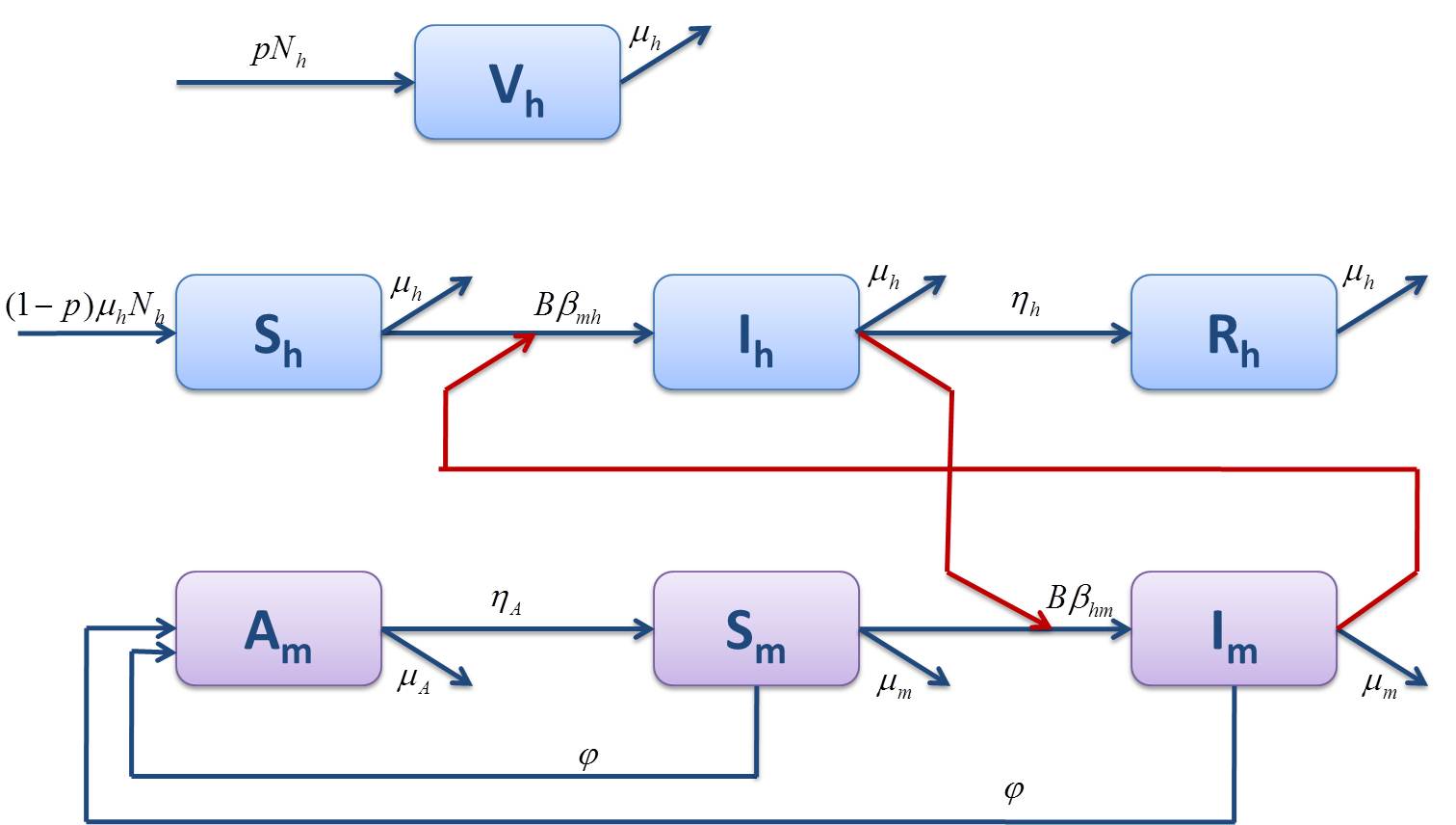
Figure 1: Epidemic model using a pediatric vaccine.

The mathematical formulation is:

$$\begin{cases}\frac{dS_{h}}{dt}(t)=(1-p)\mu_{h}N_{h}-\left(B\beta_{mh}\frac{I_{m}(t)}{N_{h}}+\mu_{h}\right)S_{h}(t)\\ \frac{dV_{h}}{dt}(t)=p\mu_{h}N_{h}-\mu_{h}V_{h}(t)\\ \frac{dI_{h}}{dt}(t)=B\beta_{mh}\frac{I_{m}(t)}{N_{h}}S_{h}(t)-(\eta_{h}+\mu_{h})I_{h}(t)\\ \frac{dR_{h}}{dt}(t)=\eta_{h}I_{h}(t)-\mu_{h}R_{h}(t)\\ \frac{dA_{m}}{dt}(t)=\varphi\left(1-\frac{A_{m}(t)}{kN_{h}}\right)(S_{m}(t)+I_{m}(t))-\left(\eta_{A}+\mu_{A}\right)A_{m}(t)\\ \frac{dS_{m}}{dt}(t)=\eta_{A}A_{m}(t)-\left(B\beta_{hm}\frac{I_{h}(t)}{N_{h}}+\mu_{m}\right)S_{m}(t)\\ \frac{dI_{m}}{dt}(t)=B\beta_{hm}\frac{I_{h}(t)}{N_{h}}S_{m}(t)-\mu_{m}I_{m}(t).\end{cases}$$ (1)

We are assuming that the vaccine is perfect, which means that it confers life-long protection. The nontrivial disease-free equilibrium for system (1) is given by

$$S_{h}=(1-p)N_{h},\quad V_{h}=pN_{h},\quad I_{h}=0,\quad R_{h}=0,$$

$$A_{m}=\left(1-\frac{\eta_{A}+\mu_{A}}{\varphi\,\eta_{A}}\mu_{m}\right)kN_{h},\quad S_{m}=\frac{\eta_{A}}{\mu_{m}}A_{m},\quad I_{m}=0.$$

As a first step, we determine the basic reproduction number without vaccination ($p=0$).

Theorem 2.1.

Without vaccination, the basic reproduction number $\mathcal{R}_{0}$, associated to the differential system (1), is given by

$$\mathcal{R}_{0}=\sqrt{\frac{kB^{2}\beta_{hm}\beta_{mh}\left(-\eta_{A}\mu_{m}-\mu_{A}\mu_{m}+\varphi\eta_{A}\right)}{\varphi(\eta_{h}+\mu_{h})\mu_{m}^{2}}}.$$ (2)

Proof.

The proof is similar to the one presented in [13]. ∎

We do all the simulations in two scenarios: an epidemic and an endemic situation. The following values for the parameters of the differential system and initial conditions were used (Tables 1 and 2). These values are based on previous works [11, 13]. A small number of initial infected individuals ($I_{h0}=10$) is considered, to simulate an early action by the health authorities. We recall that dengue is endemic when it occurs several times in a year, and is not related with the initial value of infected individuals. Moreover, a small initial value of infected individuals in an endemic scenario is in agreement with [14]. In our work the same initial value of $I_{h}$ for both epidemic and endemic scenarios is important in order to compare the development of the disease.

Parameter	Epidemic scenario	Endemic scenario
$N_{h}$	480000	480000
$B$	0.8	0.75
$\beta_{mh}$	0.375	0.21
$\beta_{hm}$	0.375	0.21
$\mu_{h}$	$\frac{1}{71\times 365}$	$\frac{1}{71\times 365}$
$\eta_{h}$	$\frac{1}{3}$	$\frac{1}{3}$
$\mu_{m}$	$\frac{1}{10}$	$\frac{1}{10}$
$\varphi$	6	6
$\mu_{A}$	$\frac{1}{4}$	$\frac{1}{4}$
$\eta_{A}$	0.08	0.08
$m$	3	3
$k$	3	3

Table 1: Parameters values of the differential system (1).

Initial conditions	Epidemic scenario	Endemic scenario
$S_{h0}$	479990	379990
$V_{h0}$	0	0
$I_{h0}$	10	10
$R_{h0}$	0	100000
$A_{m0}$	1440000	1440000
$S_{m0}$	1440000	1440000
$I_{m0}$	0	0

Table 2: Initial conditions of the differential system (1).

Two main differences between an epidemic episode and an endemic situation were found. Firstly, in the endemic situation there was a slight decrease in the average daily biting $B$ and transmission probabilities $\beta_{mh}$ and $\beta_{hm}$, which can be explained by the fact that the mosquito may have more difficulties to find a naive individual. The second difference is concerned with the strong increase of the initial human population that is resistant to the disease. This can be explained by the fact that the disease, in an endemic situation, already creates an immune resistance to the infection, i.e., the population already has herd immunity. With our values we obtain approximately $\mathcal{R}_{0}=2.46$ and $\mathcal{R}_{0}=1.29$ for epidemic and endemic scenarios, respectively.

During an outbreak, the disease transmission assumes different behaviors, according to the distinct scenarios, as can been seen in Figure 2. In one year, the peak in an epidemic situation could reach more than 80000 cases. In contrast, in the endemic situation the curve of infected individuals has a more smooth behavior and reaches a peak less than 3000 cases. Figure 3 relates to the mosquito population. In the endemic scenario, because a substantial part of the human population is resistant to the disease, the infected mosquitoes bite a considerable percentage of resistant host and, as consequence, the disease is not transmitted.

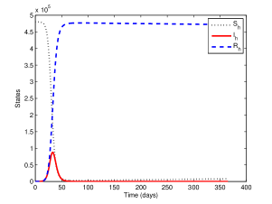
(a) Epidemic scenario

(b) Endemic scenario

Figure 2: Human population in a dengue outbreak, without vaccine.

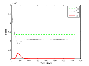
(a) Epidemic scenario

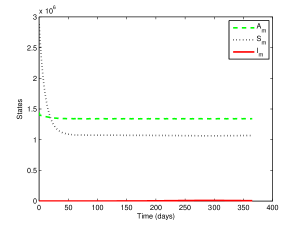
(b) Endemic scenario

Figure 3: Mosquito population in a dengue outbreak, without vaccine.

Suppose that at time $t=0$ a proportion $p$ of newborns is vaccinated with a perfect vaccine without side effects. Since this proportion, $p$, is now immune, $\mathcal{R}_{0}$ is reduced, creating a new basic reproduction number $\mathcal{R}_{0}^{p}$.

Definition 1 (cf. [1]).

The basic reproduction number with pediatric vaccination, $\mathcal{R}_{0}^{p}$, associated to the differential system (1), is given by $\mathcal{R}_{0}^{p}=(1-p)\mathcal{R}_{0}$, where $\mathcal{R}_{0}$ is defined by (2).

Observe that $\mathcal{R}_{0}^{p}\leq\mathcal{R}_{0}$. Equality is only achieved when $p=0$, i.e., when there is no vaccination. Note that the constraint $\mathcal{R}_{0}^{p}<1$ defines implicitly a critical vaccination portion $p>p_{c}:=1-\frac{1}{\mathcal{R}_{0}}$ that must be achieved for eradication. Since vaccination entails costs, to choose the smallest coverage that achieves eradication is the best option. This way, the entire population does not need to be vaccinated in order to eradicate the disease (this is the herd immunity phenomenon). Vaccinating at the critical level $p_{c}$ does not instantly lead to disease eradication. The immunity level within the population requires time to build up and at the critical level it may take a few generations before the required herd immunity is achieved. Thus, from a public health perspective, $p_{c}$ acts as a lower bound on what should be achieved, with higher levels of vaccination leading to a more rapid elimination of the disease. Figure 4 shows simulations with different proportions of the newborns vaccinated, in both epidemic and endemic scenarios. Note that at time $t=0$ no person was vaccinated. In the epidemic situation, as the outbreak reaches a peak at the beginning of the year, the proportion of newborns vaccinated at that time is minimum and cannot influence the curve of infected individuals, giving the optical illusion of a single curve. On the other hand, in the endemic case, as the outbreak occurs later, the vaccination campaign starts to produce effects, decreasing the total number of sick humans. This last graphic illustrates that a vaccination campaign centered in newborns is a bet for the future of a country, but does not produce instantly results to fight the disease. To achieve immediate results, it is necessary to use random mass vaccination, which means that it is necessary to vaccine a significant part of the population.

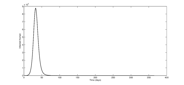
(a) Epidemic scenario

(b) Endemic scenario

Figure 4: Infected human in an outbreak, varying the proportion of newborns vaccinated ($p=0,0.25,0.50,0.75,1$).

2.2 Perfect random mass vaccination

A mass vaccination program may be initiated whenever there is an increase of the risk of an epidemic. In such situations, there is a competition between the exponential increase of the epidemic and the logistical constraints upon mass vaccination. For most human diseases it is possible, and more efficient, to not vaccinate those individuals who have recovered from the disease, because they are already protected. Another situation could be the introduction of a new vaccine in a population that lives an endemic situation. Let us consider the control technique of constant vaccination of susceptibles. In this scheme a fraction $0\leq\psi\leq 1$ of the entire susceptible population, not just newborns, is being continuously vaccinated. It is assumed that the permanent immunity acquired by vaccination is the same as natural immunity obtained from infected individuals in recovery. The epidemiological scheme is presented in Figure 5.

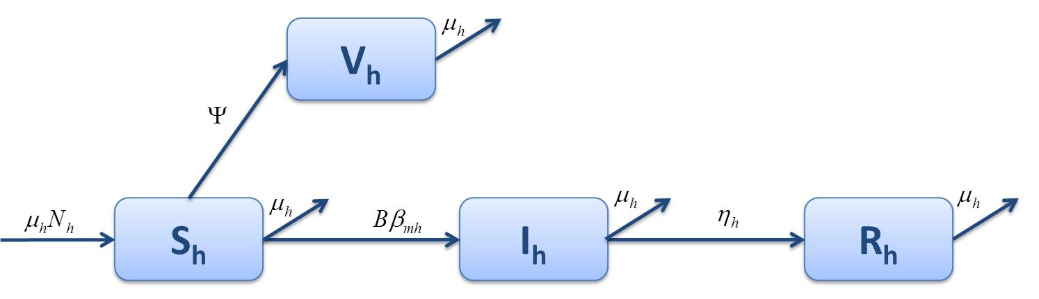
Figure 5: Epidemic model for human population using a mass random vaccine.

The mosquito population remains equal to the previous subsection, while the mathematical formulation for human population in the new epidemiological scheme is given by

$$\begin{cases}\frac{dS_{h}}{dt}(t)=\mu_{h}N_{h}-\left(B\beta_{mh}\frac{I_{m}(t)}{N_{h}}+\psi+\mu_{h}\right)S_{h}(t)\\ \frac{dV_{h}}{dt}(t)=\psi S_{h}(t)-\mu_{h}V_{h}(t)\\ \frac{dI_{h}}{dt}(t)=B\beta_{mh}\frac{I_{m}(t)}{N_{h}}S_{h}(t)-(\eta_{h}+\mu_{h})I_{h}(t)\\ \frac{dR_{h}}{dt}(t)=\eta_{h}I_{h}(t)-\mu_{h}R_{h}(t).\end{cases}$$ (3)

For this model, we define a new basic reproduction number $\mathcal{R}_{0}^{\psi}$.

Definition 2 (cf. [15]).

The basic reproduction number with random mass vaccination, $\mathcal{R}_{0}^{\psi}$, associated to the differential system (3), is given by

$$\mathcal{R}_{0}^{\psi}=\mathcal{R}_{0}\left(\frac{\mu_{h}}{\mu_{h}+\psi}\right),$$ (4)

where $\mathcal{R}_{0}$ is defined by (2).

Comparing this model with the model of constant vaccination of newborns, it is apparent that instead of constantly vaccinating a portion of newborns, a part of the entire susceptible population is now being continuously vaccinated. Since the natural birth rate $\mu_{h}$ is usually small, the fraction $p\mu_{h}$ of newborns being continuously vaccinated will be also small, whereas in this model, a larger group $\psi S_{h}$ of susceptible can be continuously vaccinated. For this reason, we expect this model to require a smaller proportion $\psi$ to achieve eradication. Note that $\mathcal{R}_{0}^{\psi}\leq\mathcal{R}_{0}$. Equality is only achieved in the limit, when $\psi=0$, that is, when there is no vaccination. The constraint $\mathcal{R}_{0}^{\psi}<1$ defines implicitly a critical vaccination portion $\psi>\psi_{c}$ that must be achieved for eradication:

$$\psi_{c}=\left(\mathcal{R}_{0}-1\right)\mu_{h}.$$

Figure 6 illustrates the variation of the number of infected people when a mass vaccination is introduced. The graphs present five simulations using different proportions of the susceptible being vaccinated: $\psi=0.05,0.10,0.25,0.50,1$. Observe that, in spite of the calculations being done in the period of 365 days, the figures only show suitable windows, in order to provide a better analysis. In both epidemic and endemic scenarios, even with a small coverage of the population, vaccination dramatically decreases the number of infected. In the epidemic scenario, the situation has changed from around 80000 cases (with no vaccination, Figure 2) to less than 1200 cases, vaccinating only 5% of the susceptible. In the endemic scenario, the decrease is even more accentuated.

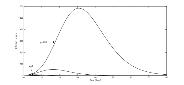
(a) Epidemic scenario

(b) Endemic scenario

Figure 6: Infected human in an outbreak, varying the proportion of susceptible population vaccinated ($\psi=0.05,0.10,0.25,0.50,1$).

Until here, we have considered a perfect vaccine, which means that every vaccinated individual remains resistant to the disease. However, a majority of the available vaccines for the human population does not produce 100% success in the disease battle. Usually, the vaccines are imperfect, which means that a minor percentage of cases, in spite of vaccination, are infected.

2.3 Imperfect random mass vaccination

Most of the theory about disease evolution is based on the assumption that the host population is homogeneous. Individual hosts, however, may differ and they may constitute very different habitats. In particular, some habitats may provide more resources or be more vulnerable to virus exploitation [16]. The use of models with imperfect vaccines can describe better this type of human heterogeneity. Another explanation for the use of imperfect vaccines is that until now we had considered models assuming that as soon as individuals begin the vaccination process, they become immediately immune to the disease. However, the time it takes for individuals to obtain immunity by completing a vaccination process cannot be ignored, because meanwhile an individual can be infected. In this section a continuous vaccination strategy is considered, where a fraction $\psi$ of the susceptible class was vaccinated. The vaccination may reduce but not completely eliminate susceptibility to infection. For this reason, we consider a factor $\sigma$ as the infection rate of vaccinated members. When $\sigma=0$, the vaccine is perfectly effective, when $\sigma=1$, the vaccine has no effect at all. The value $1-\sigma$ can be understood as the efficacy level of the vaccine. The new model for the human population is represented in Figure 7.

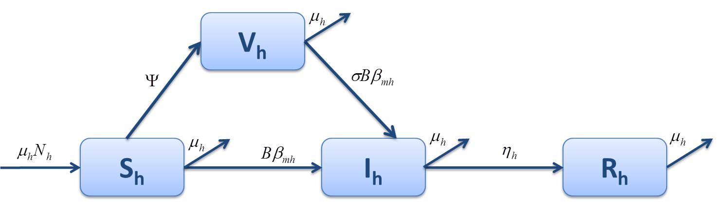
Figure 7: Epidemiological $SVIR$ model for human population with an imperfect vaccine.

Accordingly, we have the following system of differential equations:

$$\begin{cases}\frac{dS_{h}}{dt}=\mu_{h}N_{h}-\left(B\beta_{mh}\frac{I_{m}}{N_{h}}+\psi+\mu_{h}\right)S_{h}\\ \frac{dV_{h}}{dt}=\psi S_{h}-\left(\sigma B\beta_{mh}\frac{I_{m}}{N_{h}}+\mu_{h}\right)V_{h}\\ \frac{dI_{h}}{dt}=B\beta_{mh}\frac{I_{m}}{N_{h}}(S_{h}+\sigma V_{h})-(\eta_{h}+\mu_{h})I_{h}\\ \frac{dR_{h}}{dt}=\eta_{h}I_{h}-\mu_{h}R_{h}.\end{cases}$$ (5)

As expected, a new basic reproduction number is associated to (5).

Definition 3 (cf. [17]).

The basic reproduction number with an imperfect vaccine, $\mathcal{R}_{0}^{\sigma}$, associated to the differential system (5), is defined by

$$\mathcal{R}_{0}^{\sigma}=\left(1+\sigma\psi\right)\frac{\mu_{h}}{\mu_{h}+\psi}\mathcal{R}_{0}=\left(1+\sigma\psi\right)\mathcal{R}_{0}^{\psi},$$

where $\mathcal{R}_{0}^{\psi}$ is given by (4).

Note that $\mathcal{R}_{0}^{\psi}\leq\mathcal{R}_{0}^{\sigma}$ and when the vaccine is perfect, i.e., $\sigma=0$, $\mathcal{R}_{0}^{\sigma}$ degenerates into $\mathcal{R}_{0}^{\psi}$. In other words, a high efficacy vaccine leads to a lower vaccination coverage to eradicate the disease. However, it is realized in [17] that it is much more difficult to increase the efficacy level of the vaccine when compared to controlling the vaccination rate $\psi$. Figures 8 and 9 show several simulations, by varying the vaccine efficacy and the percentage of population that is vaccinated. Comparing with Figure 6a, in the epidemic scenario with a perfect vaccine, the number of human infected has reached to a maximum peak of 1200 cases per day, in the worst scenario ($\psi=0.05$). Using an imperfect vaccine, with a level of efficacy of 80% (Figure 8a), with the same values for $\psi$, the maximum peak increases until 9000 cases. We conclude that the production of a vaccine with a high level of efficacy has a preponderant role in the reduction of the disease spread. Figures 9a and 9b reinforce the previous sentence. Assuming that 85% of the population is vaccinated, the number of infected cases decreases sharply with the increasing of the effectiveness level of the vaccine.

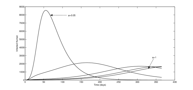
(a) Epidemic scenario

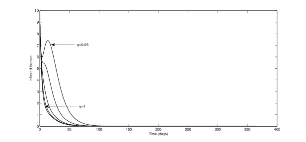
(b) Endemic scenario

Figure 8: Infected humans in an outbreak varying the proportion of susceptible population vaccinated ($\psi=0.05,0.10,0.25,0.50,1$) with a vaccine simulating 80% of effectiveness ($\sigma=0.2$)

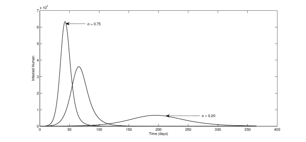
(a) Epidemic scenario

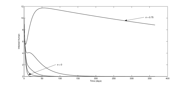
(b) Endemic scenario

Figure 9: Infected humans in an outbreak varying the efficacy level of the vaccine ($\sigma=0,0.10,0.20,0.50,0.75$) and considering that 85% of the human susceptible population is vaccinated ($\psi=0.85$).

According to [18], an acceptable level of efficacy is at least 80% against all four serotypes, and 3 to 5 for the length of protection. These values are commonly considered, across countries, as the minimum acceptable levels.

Next we study another type of imperfect vaccine: one that confers a limited life-long protection.

2.4 Random mass vaccination with waning immunity

Until the 1990s, the universal assumption of mathematical models of vaccination was: there is no waning of vaccine-induced immunity. This assumption was routinely made because, for most of the major vaccines against childhood infectious diseases, it is approximately correct [1].

Suppose that the immunity, obtained by the vaccination process, is temporary. Assume that immunity has the waning rate $\theta$. Then the model for humans is given by

$$\begin{cases}\frac{dS_{h}}{dt}(t)=\mu_{h}N_{h}+\theta V_{h}(t)-\left(B\beta_{mh}\frac{I_{m}(t)}{N_{h}}+\psi+\mu_{h}\right)S_{h}(t)\\ \frac{dV_{h}}{dt}(t)=\psi S_{h}(t)-\left(\theta+\mu_{h}\right)V_{h}(t)\\ \frac{dI_{h}}{dt}(t)=B\beta_{mh}\frac{I_{m}(t)}{N_{h}}S_{h}(t)-(\eta_{h}+\mu_{h})I_{h}(t)\\ \frac{dR_{h}}{dt}(t)=\eta_{h}I_{h}(t)-\mu_{h}R_{h}(t).\end{cases}$$ (6)

This model can be represented by the epidemiological scheme of Figure 10.

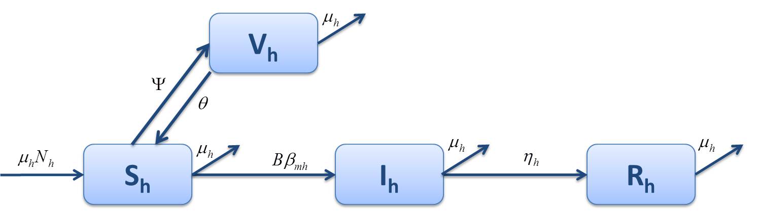
Figure 10: Epidemiological $SVIR$ model for human population with a waning immunity vaccine.

This leads naturally to the following basic reproduction number.

Definition 4.

The basic reproduction number with an imperfect vaccine, $\mathcal{R}_{0}^{\theta}$, associated to the differential system (6), is defined by $\mathcal{R}_{0}^{\theta}=\mathcal{R}_{0}^{\psi}$, where $\mathcal{R}_{0}^{\psi}$ is given by (4).

According to [19], the basic reproduction numbers $\mathcal{R}_{0}^{\theta}$ and $\mathcal{R}_{0}^{\psi}$ are the same, because the disease will still spread at the same rate with or without temporary immunity. However, we should expect that the convergence rate will be different between the random mass vaccination and random mass vaccination with waning immunity, since the disease will be eradicated faster in the constant treatment model without waning immunity compared to the other with waning immunity. Figure 11 illustrates this statement. Considering that 85% of human population is vaccinated, the number of infected is increasing as the value of the waning immunity is growing ($\theta=0,0.05,0.10,0.15,0.20$).

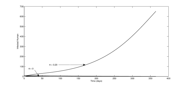
(a) Epidemic scenario

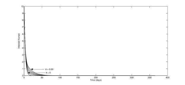
(b) Endemic scenario

Figure 11: Infected humans in an outbreak considering 85% of susceptible population vaccinated ($\psi=0.85$) and varying waning immunity $(\theta=0,0.05,0.10,0.15,0.20$).

Depending on the vaccine that will be available on the market, it will be possible to choose or even combine features. In the next section we define the vaccination process as a control system.

3 Vaccine as a control

In this section we consider a SIR model for humans and an ASI model for mosquitoes. The parameters remain the same as in the previous section. The vaccination is seen as a control variable to reduce or even eradicate the disease. Let $u$ be the control variable: $0\leq u(t)\leq 1$ denotes the percentage of susceptible individuals that one decides to vaccinate at time $t$. A random mass vaccination with waning immunity is selected. In this way, a parameter $\theta$ associated to the control $u$ represents the waning immunity process. Figure 12 shows the epidemiological scheme for the human population. Note that $R_{h}$ includes both vaccinated and naturally-immune individuals; only vaccinated immune individuals have waning immunity.

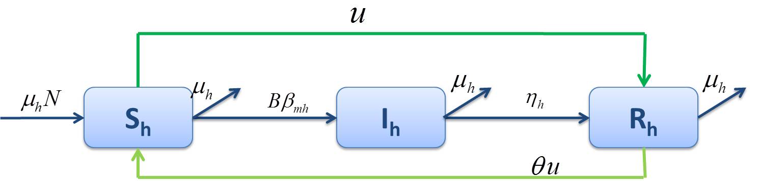
Figure 12: Epidemiological $SIR$ model for the human population using the vaccine as a control.

The model is described by an initial value problem with a system of six differential equations:

$$\begin{cases}\frac{dS_{h}}{dt}=\mu_{h}N_{h}-\left(B\beta_{mh}\frac{I_{m}}{N_{h}}+\mu_{h}+u\right)S_{h}+\theta uR_{h}\\ \frac{dI_{h}}{dt}=B\beta_{mh}\frac{I_{m}}{N_{h}}S_{h}-(\eta_{h}+\mu_{h})I_{h}\\ \frac{dR_{h}}{dt}=\eta_{h}I_{h}+uS_{h}-\left(\theta u+\mu_{h}\right)R_{h}\\ \frac{dA_{m}}{dt}=\varphi\left(1-\frac{A_{m}}{kN_{h}}\right)(S_{m}+I_{m})-\left(\eta_{A}+\mu_{A}\right)A_{m}\\ \frac{dS_{m}}{dt}=\eta_{A}A_{m}-\left(B\beta_{hm}\frac{I_{h}}{N_{h}}+\mu_{m}\right)S_{m}\\ \frac{dI_{m}}{dt}=B\beta_{hm}\frac{I_{h}}{N_{h}}S_{m}-\mu_{m}I_{m}.\end{cases}$$ (7)

The main aim is to study the optimal vaccination strategy, considering both the costs of treatment of infected individuals and the costs of vaccination. The objective is to

$$\text{ minimize }J[u]=\int_{0}^{t_{f}}\left[\gamma_{D}I_{h}(t)^{2}+\gamma_{V}u(t)^{2}\right]dt,$$ (8)

where $\gamma_{D}$ and $\gamma_{V}$ are positive constants representing the weights of the costs of treatment of infected people and vaccination, respectively. We solve the problem using optimal control theory.

3.1 Pontryagin’s Maximum Principle

Let us consider the following set of admissible control functions:

$$\Delta=\{u(\cdot)\in L^{\infty}(0,t_{f})\,|\,0\leq u(t)\leq 1,\forall t\in[0,t_{f}]\}.$$

Theorem 3.1.

The problem (7)–(8) with initial conditions (see Table 2), admits a unique optimal solution $\left(S_{h}^{*}(\cdot),I_{h}^{*}(\cdot),R_{h}^{*}(\cdot),A_{m}^{*}(\cdot),S_{m}^{*}(\cdot),I_{m}^{*}(\cdot)\right)$ associated with an optimal control $u^{*}(\cdot)$ on $[0,t_{f}]$, with a fixed final time $t_{f}$. Moreover, there exists adjoint functions $\lambda_{i}^{*}(\cdot)$, $i=1,\ldots,6$, satisfying

$$\left\{\begin{array}[]{l}\dot{\lambda}_{1}^{*}(t)=(\lambda_{1}-\lambda_{2})\left(B\beta_{mh}\frac{I_{m}(t)}{N_{h}}\right)+\lambda_{1}\mu_{h}+(\lambda_{1}-\lambda_{3})u(t)\\ \dot{\lambda}_{2}^{*}(t)=-2\gamma_{D}I_{h}(t)+\lambda_{2}(\eta_{h}+\mu_{h})-\lambda_{3}\eta_{h}+(\lambda_{5}-\lambda_{6})\left(B\beta_{hm}\frac{S_{m}(t)}{N_{h}}\right)\\ \dot{\lambda}_{3}^{*}(t)=-\lambda_{1}\theta u(t)+\lambda_{3}(\mu_{h}+\theta u(t))\\ \dot{\lambda}_{4}^{*}(t)=\lambda_{4}\varphi\frac{S_{m}(t)+I_{m}(t)}{kN_{h}}+\lambda_{4}(\eta_{A}+\mu_{A})-\lambda_{5}\eta_{A}\\ \dot{\lambda}_{5}^{*}(t)=-\lambda_{4}\varphi\left(1-\frac{A_{m}(t)}{kN_{h}}\right)+(\lambda_{5}-\lambda_{6})B\beta_{hm}\frac{I_{h}(t)}{N_{h}}+\lambda_{5}\mu_{m}\\ \dot{\lambda}_{6}^{*}(t)=(\lambda_{1}-\lambda_{2})\left(B\beta_{mh}\frac{S_{h}(t)}{N_{h}}\right)-\lambda_{4}\varphi\left(1-\frac{A_{m}(t)}{kN_{h}}\right)+\lambda_{6}\mu_{m}\\ \end{array}\right.$$

(9)

and the transversality conditions $\lambda_{i}^{*}(t_{f})=0$, i=1, …6. Furthermore,

$$u^{*}(t)=\min\left\{1,\max\left\{0,\frac{\left(\lambda_{1}(t)-\lambda_{3}(t)\right)\left(S_{h}(t)-\theta R_{h}(t)\right)}{2\gamma_{V}}\right\}\right\}.$$ (10)

Proof.

The existence of optimal solutions $\left(S_{h}^{*}(\cdot),I_{h}^{*}(\cdot),R_{h}^{*}(\cdot),A_{m}^{*}(\cdot),S_{m}^{*}(\cdot),I_{m}^{*}(\cdot)\right)$ associated to the optimal control $u^{*}(\cdot)$ comes from the convexity of the integrand of the cost functional (8) with respect to the control $u$ and the Lipschitz property of the state system with respect to state variables $\left(S_{h},I_{h},R_{h},A_{m},S_{m},I_{m}\right)$ (for more details, see [20, 21]). According to the Pontryagin maximum principle [22], if $u^{*}(\cdot)\in\Delta$ is optimal for the problem considered, then there exists a nontrivial absolutely continuous mapping $\lambda:[0,t_{f}]\rightarrow\mathbb{R}$, $\lambda(t)=\left(\lambda_{1}(t),\lambda_{2}(t),\lambda_{3}(t),\lambda_{4}(t),\lambda_{5}(t),\lambda_{6}(t)\right)$, called the adjoint vector, such that

$$\dot{S}_{h}=\frac{\partial H}{\partial\lambda_{1}},\quad\dot{I}_{h}=\frac{\partial H}{\partial\lambda_{2}},\quad\dot{R}_{h}=\frac{\partial H}{\partial\lambda_{3}},\quad\dot{A}_{m}=\frac{\partial H}{\partial\lambda_{4}},\quad\dot{S}_{m}=\frac{\partial H}{\partial\lambda_{5}},\quad\dot{I}_{m}=\frac{\partial H}{\partial\lambda_{6}}$$ (11)

and

$$\dot{\lambda}_{1}=-\frac{\partial H}{\partial S_{h}},\quad\dot{\lambda}_{2}=-\frac{\partial H}{\partial I_{h}},\quad\dot{\lambda}_{3}=-\frac{\partial H}{\partial R_{h}},\quad\dot{\lambda}_{4}=-\frac{\partial H}{\partial A_{m}},\quad\dot{\lambda}_{5}=-\frac{\partial H}{\partial S_{m}},\quad\dot{\lambda}_{6}=-\frac{\partial H}{\partial I_{m}},$$ (12)

where the Hamiltonian $H$ is defined by

$$\begin{split}H(S_{h},I_{h},R_{h},&A_{m},S_{m},I_{m},\lambda,u)=\gamma_{D}I_{h}^{2}+\gamma_{V}u^{2}+\lambda_{1}\left(\mu_{h}N_{h}-\left(B\beta_{mh}\frac{I_{m}}{N_{h}}+\mu_{h}+u\right)S_{h}+\theta uR_{h}\right)\\ &+\lambda_{2}\left(B\beta_{mh}\frac{I_{m}}{N_{h}}S_{h}-(\eta_{h}+\mu_{h})I_{h}\right)+\lambda_{3}\left(\eta_{h}I_{h}+uS_{h}-(\theta u+\mu_{h})R_{h}\right)\\ &+\lambda_{4}\left(\varphi\left(1-\frac{A_{m}}{kN_{h}}\right)(S_{m}+I_{m})-\left(\eta_{A}+\mu_{A}\right)A_{m}\right)\\ &+\lambda_{5}\left(\eta_{A}A_{m}-\left(B\beta_{hm}\frac{I_{h}}{N_{h}}+\mu_{m}\right)S_{m}\right)+\lambda_{6}\left(B\beta_{hm}\frac{I_{h}}{N_{h}}S_{m}-\mu_{m}I_{m}\right),\end{split}$$

together with the minimality condition

$$H\left(S_{h}^{*}(t),I_{h}^{*}(t),R_{h}^{*}(t),A_{m}^{*}(t),S_{m}^{*}(t),I_{m}^{*}(t),\lambda^{*}(t),u^{*}(t)\right)\\ =\min_{u}H\left(S_{h}^{*}(t),I_{h}^{*}(t),R_{h}^{*}(t),A_{m}^{*}(t),S_{m}^{*}(t),I_{m}^{*}(t),\lambda^{*}(t),u\right),$$ (13)

satisfied almost everywhere on $[0,t_{f}]$. Moreover, the transversality conditions $\lambda_{i}(t_{f})=0$ hold, $i=1,\ldots 6$. System (9) is derived from (12), and the optimal control (10) comes from the minimality condition (13). ∎

3.2 Numerical simulations and discussion

The simulations were carried out using the values of Section 2. The values chosen for the weights in the objective functional (8) were $\gamma_{D}=0.5$ and $\gamma_{V}=0.5$. The system was normalized, putting all variables varying from 0 to 1. It was considered that the waning immunity was at a rate of $\theta=0.05$. The optimal control problem was solved using two methods: direct [23, 24] and indirect [25]. The direct method uses the cost functional (8) and the state system (7) and was solved by DOTcvp [26]. The indirect method used is an iterative method with a Runge–Kutta scheme, solved through ode45 of MatLab. Figure 13 shows the optimal control obtained by both methods. Note that DOTcvp only gives the optimal control as a constant piecewise function. Table 3 shows the costs obtained by the two methods in both scenarios. The indirect method gives a lower cost. This method uses more mathematical theory about the problem, such as the adjoint system (11) and optimal control expression (10). Therefore, it makes sense that the indirect method produces a better result.

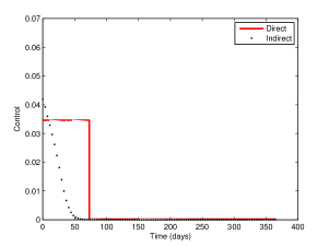
(a) Epidemic scenario

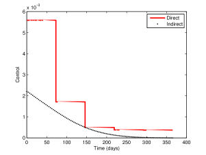
(b) Endemic scenario

Figure 13: Optimal control obtained from direct and indirect approaches, in both epidemic and endemic scenarios.

Method	Epidemic scenario	Endemic scenario
Direct (DOTcvp)	0.07505791	0.00189056
Indirect (backward-forward)	0.06070556	0.00080618

Table 3: Optimal values of the cost functional (8).

Using the optimal solution as reference, some tests were performed, regarding infected individuals and costs, when no control ($u\equiv 0$) or upper control ($u\equiv 1$) is applied. Table 4 shows the results for DOTcvp in the three situations. In both scenarios, using the optimal strategy of vaccination produces better costs with the disease, when compared to not doing anything. Once there is no control, the number of infected humans is higher and produces a more expensive cost functional. Figure 14 shows the number of infected humans when different controls are considered. It is possible to see that using the upper control, which means that everyone is vaccinated, implies that just a few individuals were infected, allowing eradication of the disease. Although the optimal control, in the sense of objective (8), allows the occurrence of an outbreak, the number of infected individuals is much lower when compared with a situation where no one is vaccinated.

	Epidemic scenario	Endemic scenario
optimal control	0.07505791	0.00189056
no control	0.32326592	0.01045990
upper control	147.82500296	116.800000275

Table 4: Values of the cost functional with optimal control, no control ($u\equiv 0$), and upper control ($u\equiv 1$).

(a) Epidemic scenario

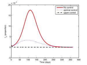
(b) Endemic scenario

Figure 14: Infected humans when using the optimal vaccination strategy, in terms of (8), no vaccination ($u\equiv 0$), and vaccination of all susceptible population ($u\equiv 1$).

We conclude that, assuming a considerable efficacy level of the vaccine, a vaccination campaign in the susceptible population can quickly decrease the number of infected people. Figures 15 and 16 show what happens to the optimal solution, in the epidemic and endemic scenarios, respectively, when the efficacy is changed. These figures confirm an increasing of infected human and control application with an increasing of the waning immunity rate $\theta$.

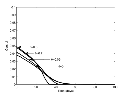
(a) Optimal control

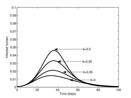
(b) Number of infected

Figure 15: Optimal solutions for different vaccine efficacies (epidemic scenario).

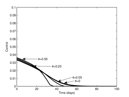
(a) Optimal control

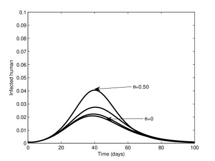
(b) Number of infected

Figure 16: Optimal solutions for different vaccine efficacies (endemic scenario).

4 Conclusions

The worldwide expansion of dengue fever is a growing health problem. In Portugal, on October 2012, for the first time in its history, an outbreak of dengue on the Madeira island occurred. Besides Aedes albipictus, the other vector that transmits the disease is already in the Old Continent, namely in Italy and Spain. Dengue vaccine is an urgent challenge that needs to be overcome. This may be commercially available within a few years, when the researchers will find a formula that protect against all four dengue viruses. A vaccination program is seen as an important measure used in infectious disease control and immunization and eradication programs.

In the first part of the paper, different ways of distributing the vaccine, as well as their features and some of coverage thresholds, were introduced, in order to cover most of the future vaccine features. The main goal of a vaccination program is to reduce the prevalence of an infectious disease and ultimately to eradicate it. It was shown that eradication success depends on the type of vaccine as well as on the vaccination coverage. The imperfect vaccines may not completely prevent infection but could reduce the probability of being infected, thereby reducing the disease burden. In this study all the simulations were done using epidemic and endemic scenarios to illustrate distinct realities. A second analysis was made, using an optimal control approach. The vaccine behaved as a new disease control variable and, when available, can be a promising strategy to fight the disease.

Dengue is an infectious tropical disease difficult to prevent and manage. Researchers agree that the development of a vaccine for dengue is a question of high priority. In the present study we have shown how a vaccine results in reducing morbidity and, simultaneously, in a reduction of the budget related with the disease. As future work we intend to study the interaction of a dengue vaccine with other kinds of controls already investigated in the literature, such as insecticide and educational campaigns [13, 27]. It would be also interesting to investigate what happens if the final size of the epidemic is included in the objective functional.

References

- [1] A. Scherer, A. McLean, Mathematical models of vaccination, British Medical Bulletin 62 (1) (2002) 187–199.
- [2] C. Farrington, On vaccine efficacy and reproduction numbers, Math. Biosci. 185 (1) (2003) 89–109.
- [3] M. Otero, N. Schweigmann, H. G. Solari, A stochastic spatial dynamical model for aedes aegypti, Bull. Math. Biol. 70 (5) (2008) 1297–1325.
- [4] P. Cattand, et al., Disease Control Priorities in Developing Countries, DCPP Publications, 2006, Ch. Tropical Diseases Lacking Adequate Control Measures: Dengue, Leishmaniasis, and African Trypanosomiasis, pp. 451–466.
- [5] M. J. Keeling, P. Rohani, Modeling infectious diseases in humans and animals, Princeton, NJ: Princeton University Press, 2008.
- [6] S. Murrell, S. C. Wu, M. Butler, Review of dengue virus and the development of a vaccine, Biotechnology Advances 29 (2) (2011) 239–247.
- [7] D. V. Clark, et al., Economic impact of dengue fever / dengue hemorrhagic fever in Thailand at the family and population levels, Am J Trop Med Hyg 72 (6) (2005) 786–791.
- [8] D. S. Shepard, et al., Cost-effectiveness of a pediatric dengue vaccine, Vaccine 22 (9-10) (2004) 1275–1280.
- [9] J. A. Suaya, et al., Cost of dengue cases in eight countries in the Americas and Asia: A prospective study, Am J Trop Med Hyg 80 (5) (2009) 846–855.
- [10] A. K. Supriatna, E. Soewono, S. A. Van Gils, A two-age-classes dengue transmission model, Mathematical Biosciences 216 (1) (2008) 114–121.
- [11] H. S. Rodrigues, M. T. T. Monteiro, D. F. M. Torres, Modeling and optimal control applied to a vector borne disease, in: J. Vigo-Aguiar (Ed.), Proceedings of the 2012 International Conference on Computational and Mathematical Methods in Science and Engineering, Vol. III, 2012, pp. 1063–1070. arXiv:1207.1949
- [12] Y. Dumont, F. Chiroleu, Vector control for the Chikungunya disease, Math. Biosci. Eng. 7 (2) (2010) 313–345.
- [13] H. S. Rodrigues, M. T. T. Monteiro, D. F. M. Torres, A. Zinober, Dengue disease, basic reproduction number and control, Int. J. Comput. Math. 89 (3) (2012) 334–346. arXiv:1103.1923
- [14] L. C. de Castro Medeiros, C. A. R. Castilho, C. Braga, W. V. de Souza, L. Regis, A. M. V. Monteiro, Modeling the dynamic transmission of dengue fever: investigating disease persistence, PLoS Negl. Trop. Dis. 5 (1) (2011) e942, 14 pp.
- [15] Y. Zhou, H. Liu, Stability of periodic solutions for an sis model with pulse vaccination, Mathematical and Computer Modelling 38 (2003) 299–308.
- [16] S. Gandon, M. Mackinnon, S. Nee, A. Read, Imperfect vaccination: some epidemiological and evolutionary consequences, in: Proceedings of Biological Sciences, Vol. 270, 2003, pp. 1129–1136.
- [17] X. Liu, Y. Takeuchib, S. Iwami, SVIR epidemic models with vaccination strategies, Journal of Theoretical Biology 253 (2008) 1–11.
- [18] D. DeRoeck, J. Deen, J. D. Clemens, Policymakers’ views on dengue fever/dengue haemorrhagic fever and the need for dengue vaccines in four southeast Asian countries, Vaccine 22 (2003) 121–129.
- [19] P. Stechlinski, A study of infectious disease models with switching, Ph.D. thesis, University of Waterloo (2009).
- [20] L. Cesari, Optimization — theory and applications. Problems with ordinary differential equations, Applications of Mathematics, 17, New York, Heidelberg-Berlin: Springer-Verlag, 1983.
- [21] C. J. Silva, D. F. M. Torres, Optimal control strategies for tuberculosis treatment: a case study in Angola, Numer. Algebra Control Optim. 2 (3) (2012) 601–617. arXiv:1203.3255
- [22] L. S. Pontryagin, V. G. Boltyanskii, R. V. Gamkrelidze, E. F. Mishchenko, The mathematical theory of optimal processes, Translated from the Russian by K. N. Trirogoff; edited by L. W. Neustadt, Interscience Publishers John Wiley & Sons, Inc. New York-London, 1962.
- [23] J. Betts, Practical Methods for Optimal Control Using Nonlinear Programming, SIAM: Advances in Design and Control, 2001.
- [24] E. Trélat, Contrôle optimal: théorie & applications, Vuibert, Collection Mathématiques Concrètes, 2005.
- [25] S. Lenhart, J. T. Workman, Optimal control applied to biological models, Chapman & Hall/CRC Mathematical and Computational Biology Series, Chapman & Hall/CRC, Boca Raton, FL, 2007.
- [26] T. Hirmajer, E. Balsa-Canto, J. R. Banga, Dotcvpsb, a software toolbox for dynamic optimization in systems biology, Bioinformatics 10 (2009) 199–213.
- [27] H. S. Rodrigues, M. T. T. Monteiro, D. F. M. Torres, Insecticide control in a dengue epidemics model, in: T. E. Simos, et al. (Eds.), Numerical analysis and applied mathematics. International conference on numerical analysis and applied mathematics, Rhodes, Greece. American Institute of Physics Conf. Proc., no. 1281 in American Institute of Physics Conf. Proc., 2010, pp. 979–982. arXiv:1007.5159