Microscopically based calculations of the free energy barrier and dynamic length scale in supercooled liquids:
The comparative role of configurational entropy and elasticity

Abstract

We compute the temperature-dependent barrier for $\alpha$-relaxations in several liquids, without adjustable parameters, using experimentally determined elastic, structural, and calorimetric data. We employ the random first order transition (RFOT) theory, in which relaxation occurs via activated reconfigurations between distinct, aperiodic minima of the free energy. Two different approximations for the mismatch penalty between the distinct aperiodic states are compared, one due to Xia and Wolynes (Proc. Natl. Acad. Sci. 97, 2990), which scales universally with temperature as for hard spheres, and one due to Rabochiy and Lubchenko (J. Chem. Phys. 138, 12A534), which employs measured elastic and structural data for individual substances. The agreement between the predictions and experiment is satisfactory, given the uncertainty in the measured experimental inputs. The explicitly computed barriers are used to calculate the glass transition temperature for each substance—a kinetic quantity—from the static input data alone. The temperature dependence of both the elastic and structural constants enters the temperature dependence of the barrier over an extended range to a degree that varies from substance to substance. The lowering of the configurational entropy, however, seems to be the dominant contributor to the barrier increase near the laboratory glass transition, consistent with previous experimental tests of the RFOT theory using the XW approximation. In addition, we compute the temperature dependence of the dynamical correlation length, also without using adjustable parameters. These agree well with experimental estimates obtained using the Berthier et al.(Science 310, 1797) procedure. Finally, we find the temperature dependence of the complexity of a rearranging region is consistent with the picture based on the RFOT theory but is in conflict with the assumptions of the Adam-Gibbs and “shoving” scenarios for the viscous slowing down in supercooled liquids.

I Motivation

There is little consensus, at present, on the detailed connection between the molecular motions preceding the glass transition and system-specific interactions, in actual glass-formers. The uncertainties are such that wildly different hypotheses about the underlying physics are still entertainedBiroli and Garrahan (2013), despite much recent progressLubchenko and Wolynes (2007a). The ambiguity in complete molecular understanding also prevents one from calculating the liquid relaxation rates and the glass-forming ability for specific substances, making materials design difficult. Of course, such difficulties are part of the bigger challenge—still faced by materials scientists of all stripes—that of the à priori prediction of the structure and phase behavior of compounds with arbitrary stoichiometries.

Despite these issues, a microscopic foundation to address quantitatively the structure and dynamics of supercooled liquids has been provided by the random first order transition (RFOT) theory, see Ref.Lubchenko and Wolynes (2007a) for a review. In this picture, the transport in the liquid above its glass transition is realized by local, activated reconfiguration events between long-lived, quasi-equilibrium aperiodic structures. It is the central notion of the ROFT theory that sufficiently below the crossover to activated transport, these reconfigurations take place by a process resembling nucleation of a new aperiodic arrangement within the one presently existing, according to the following free energy profileKirkpatrick et al. (1989); Xia and Wolynes (2000):

$$F(r)=4\pi r^{2}\sigma_{0}(a/r)^{1/2}-(4\pi/3)(r/a)^{3}Ts_{c},$$ (1)

where the first term on the right hand side represents the mismatch penalty between the initial and final configuration. The scaling of the penalty with the droplet size $r$ as $r^{3/2}$—not the familiar $r^{2}$—implies, effectively, a curvature dependent surface tension coefficient $\sigma=\sigma_{0}(a/r)^{1/2}$Kirkpatrick et al. (1989); Villain (1985). The quantity $\sigma_{0}$ is the mismatch penalty at length scale $a$ equal to the volumetric size of the chemically rigid molecular unit, or “bead”Lubchenko and Wolynes (2003); Bevzenko and Lubchenko (2009). The second term on the right hand side gives the bulk-driving force for the reconfiguration, which, in equilibrium, is completely determined by the excess, configurational entropy of the liquid, denoted here as $s_{c}$, per bead. The driving force also has an enthalpic component during aging, where the initial state has stored energyLubchenko and Wolynes (2004).

The free energy profile (1) yields the following activation barrierKirkpatrick et al. (1989); Xia and Wolynes (2000):

$$\frac{F^{\ddagger}}{k_{B}T}=\frac{3\pi(\sigma_{0}a^{2}/k_{B}T)^{2}}{s_{c}/k_{B}}.$$ (2)

Furthermore, the size $r^{*}$ such that $F(r^{*})=0$ corresponds to a region that typically has an alternative state. Thus it represents the cooperativity length for the reconfigurations. Often, one uses a volumetric size $\xi\equiv(4\pi/3)^{1/3}r^{*}$. From Eq. (1), it follows that

$$\xi/a=(4\pi/3)^{1/3}\left(\frac{3\sigma_{0}a^{2}}{Ts_{c}}\right)^{2/3}.$$ (3)

According to Eq. (3), the cooperativity size is determined by a competition between two factors: the free energy cost of extending the interface between alternative aperiodic states and their multiplicity. Eq. (2) shows that the temperature dependences of these two competing factors determine the temperature dependence of the activation barrier.

The configurational entropy can, in principle, be calculated for actual substances starting from the force laws by using the classical density functional theoryHall and Wolynes (2008) or recent replica-approachesMézard and Parisi (1999); Parisi and Zamponi (2010). In practice, making such estimates is quite challenging for molecules that are not spherically shaped. At any rate, a good approximation to $s_{c}$ can be determined by integrating the calorimetrically determined heat capacity of the glass and the supercooled liquidL.-M. Martinez and Angell (2001); Angell (1997).

The mismatch penalty, or the surface tension coefficient $\sigma_{0}$, cannot be measured directly in the laboratory, but again a recipe exists for calculating it from first principles. The DFT formalism does suggest some simple approximations. Xia and WolynesXia and Wolynes (2000) (XW) put forth a general argument, by which the mismatch penalty is approximated by the free energy cost of “localizing” individual particles during the crossover to the activated transportXia and Wolynes (2000), see also the discussion of Eq. (9) in Ref.Rabochiy and Lubchenko (2013). As such, the penalty is largely determined by the kinetic pressure—which, in turn, scales approximately linearly with the ambient temperature (it does so exactly for hard spheres)—and the logarithm of the vibrational displacement of a particle around its average position in the aperiodic lattice. This yields the following, very simple formula for the activation barrier $F^{\ddagger}$ in equilibriumXia and Wolynes (2000); Lubchenko and Wolynes (2003); Stevenson and Wolynes (2005):

$$\frac{F^{\ddagger}}{k_{B}T}\approx\frac{32.k_{B}}{s_{c}}.$$ (4)

In the assumption that the surface tension coefficient $\sigma_{0}$ in Eqs. (1) and (2) changes smoothly with temperature, the above expression can be regarded as an asymptotic result that is expected to work better the closer the system is to the “ideal glass transition” at the KauzmannKauzmann (1948) temperature $T_{K}$. Below $T_{K}$, the glass is in a putative state for which the multiplicity of the distinct aperiodic packings is subthermodynamic so that the configurational entropy vanishes. This ideal glass state is not achievable by cooling directly, owing to the diverging relaxation times; it is also predicted generally to be avoided by substances that can crystallize into a periodic structureStevenson and Wolynes (2011). Although expected to be strictly correct only asymptotically, the formalism leading to Eq. (4) has given rise to dozens of quantitative predictions of seemingly disparate glassy phenomena, without making use of adjustable parameters. One of these is the “fragility index”:

$$m=\frac{\partial\log_{10}\tau}{\partial(T_{g}/T)}\Big{|}_{T=T_{g}}.$$ (5)

By Eq. (4), the XW estimate of the mismatch penalty impliesLubchenko and Wolynes (2003); Stevenson and Wolynes (2005)

$$m_{\text{frag}}\approx 20.7\Delta c_{p}/k_{B},$$ (6)

where $\Delta c_{p}$ is the heat capacity jump at the glass transition. The numerical constant 20.7 pertains specifically to setting the laboratory glass transition to occur on the time scale $10^{5}$ sec, see below for derivation. The constant would be (modestly) different for other speeds of quenching. The simple relation (6) between the kinetic and thermodynamic attributes of the glass transition does indeed conform to observation, according to the compilation of several dozen substances by Stevenson and WolynesStevenson and Wolynes (2005), even though it appears to systematically underestimate the fragility for the more fragile substances.

Dozens more predictions stemming from the XW estimate for the mismatch energy factor $\sigma_{0}$ have been confirmed by experiment and include, importantly, the size of the cooperative reconfigurationsAshtekar et al. (2010); Tracht et al. (1998); Russell and Israeloff (2000); Cicerone and Ediger (1996); Berthier et al. (2005), see Refs.Lubchenko and Wolynes (2007a, b); Lubchenko (2012); Lubchenko and Wolynes (2012) for reviews, and also more recent work in Refs.Wisitsorasak and Wolynes (2012); Rabochiy and Lubchenko (2012a, b, 2013); Wisitsorasak and Wolynes (2013). Note that the strict existence of the ideal glass state is not necessary for the RFOT theory to be useful, although quantitative predictions are expected to be the more accurate the smaller the value of $s_{c}$, as already mentioned. Recently, ultrastable glasses have been produced by vapor deposition that are characterized by values of $s_{c}$Swallen et al. (2007); Dawson et al. (2009); Stevenson and Wolynes (2008), that are significantly lower than at the common laboratory $T_{g}$ achieved by cooling. The predictions of the ROFT theory still seem to hold up since the limiting configurational entropy predicted by surface motions in the RFOT theory is confirmed. It is also important to recognize that there is a rigorous sense, in which the entropy crisis at $T_{K}$ exists as a possible idealized fixed point, as has been shown in related spin modelsKirkpatrick and Wolynes (1987) and via liquid theory approximations of Parisi and coworkersMézard and Parisi (1999); Parisi and Zamponi (2010).

Recently, Rabochiy and LubchenkoRabochiy and Lubchenko (2013) (RL) have estimated the mismatch penalty in a different way, using a more detailed density functional argument than XW employed. In their argument, the activation barrier explicitly depends on the high-frequency elastic moduli of the liquid and local coordination, via the structure factor $S(k)$, in addition to the configurational entropy. The calculations of the mismatch penalty made by them for several substances were limited to the vicinity of the glass transition because the elastic constants and structure factor were not measured over sufficiently extended temperature range. Despite the complexity of the approximation in Ref.Rabochiy and Lubchenko (2013) and the potential ambiguities in the experimentally measured inputs, the values of the mismatch penalty obtained by RL near $T_{g}$ are quite close to the estimates found by XW.

Here we use both the XW and RL derived expressions for $\sigma_{0}$ to compute, for the first time, the entire temperature dependence of the activation barrier for eight specific substances, over a finite temperature range, without adjustable parameters. The calculation can be justly called microscopic even though experimental input data are used. The input parameters consist of experimentally determined configurational entropy (XW and RL), high-frequency elastic constants, and the structure factor (RL). These are all “static” quantities. In addition, we will use the entropy of fusion to independently determine the volumetric size of the chemically rigid molecular unit, or the “bead.” Unfortunately, the structure factor $S(k)$ is available only at a single temperature for most of the substances in question. We have thus been forced to use the $S(k)$ values measured at a specific fixed temperature, usually near $T_{g}$, in the full temperature range; it is possible to assess the resulting error in some cases. In addition to directly comparing to experimental relaxation times, the predictions for the barriers are also tested by computing the corresponding kinetic glass transition temperature from the input static data and comparing these against experimental data. Another quantity of interest we calculate is the fragility coefficient. Finally, the same input data are used to estimate the cooperativity length $\xi$ for the two approximations. These are then compared to the values that are essentially experimentally determined via a relation due to Berthier et al.Berthier et al. (2005). We point out that all of the input data here taken from experiment for actual molecular systems can be obtained approximately using existing theoretical formalisms for sufficiently simple systems like Lennard-Jones spheres.

Of the four predicted quantities mentioned above, the absolute barrier itself at a given temperature and the fragility, which is the rate of barrier change with temperature, appear to be most sensitive to uncertainty in the experimental inputs and potential errors of the approximations. To separate the effects of these uncertainties on the absolute value of barrier and the rate of its change with temperature, we may rescale the barrier to match its known value at $T_{g}$, which is equivalent to using one adjustable constant, say, the bead size. This rescaling—which is in general, as we shall see, quite modest—has the effect of eliminating error in the absolute value of the barrier at the laboratory $T_{g}$: Using Eq. (4) and

$$\tau=\tau_{0}e^{F^{\ddagger}/k_{B}T},$$ (7)

one obtains $m_{\text{frag}}=(\log_{10}e)[F^{\ddagger}(T_{g})/T_{g}]\Delta c_{p}(T_{g})/s_{c}(T_{g})=\Delta c_{p}(T_{g})(\log_{10}e)[\ln\tau(T_{g})/\tau_{0}]^{2}/32.$Lubchenko and Wolynes (2003); Stevenson and Wolynes (2005). The logarithm in the latter expression is fixed by the timescale of the glass transition, and so one is left only with assessing the relative temperature derivative of the barrier.

While the complete temperature dependence of the rescaled barriers does deviate somewhat from the experimental values, the discrepancy is more noticeable for strong substances, for which the temperature range between the crossover and glass transition is larger, as well as the range to the ideal glass transition. In all cases, the RL predicted barrier decreases with temperature consistently faster than does the measured barrier. At the same time, the XW expression, which leaves out the potential temperature dependence of the elastic constants, owing to its hard sphere form, consistently yields a slower decay rate of the barrier with temperature, as expected; Lubchenko and Wolynes dealt with these barrier softening effects a decade agoLubchenko and Wolynes (2003). Although the set of substances covered here is admittedly modest in number, it does cover a wide chemical and fragility range suggesting the systematic underestimation of the barrier found here is meaningful. This, in turn, implies the RL expression is an adequate stepping stone for further systematic improvements in the theory of the absolute barriers.

The present work also allows us to determine the relative contributions of the temperature dependence of the configurational entropy and the temperature dependence of the elastic constants to the barrier increase with lowering temperature, which has excited much discussionBiroli and Bouchaud (2012). The elastic constant variation is central to many non-RFOT based ideas about glassy dynamics. For instance, recent work independently indicates there is an intimate connection between the elastic constants and the translational symmetry breaking in supercooled liquidsMari et al. (2009); Yan et al. (2013). Some worksDyre and Wang (2012); Klieber et al. (2013) go as far as to suggest that the temperature dependence of the barrier is exclusively due to changes of the shear modulus and nothing else. In those scenarios, the barrier and the shear modulus are taken to be simply proportional to each other. This simplicity requires there being a fixed cooperativity length determined by some other physical principle for each substance. In the purely elastic analysis, this size is then regarded as a freely adjustable parameter. The theory does not provide a specific recipe for calculating it. In contrast, the RFOT-based approach of RL dictates that the barrier depends on the elastic constants in an intricate fashion, while the size factor is predicted from the theory itself as in the XW implementation of theory. Importantly, the RL approximation calls for the use of high-frequency elastic moduli, i.e., on times shorter than the plateau time scale of the stress relaxation function. Here we show that even within the RL approximation, which appears to overestimate the variation of the barrier with temperature, the entropic contribution to the temperature dependence of the barrier progressively dominates the elastic part with decreasing temperature. Finally, we compute the complexity of the rearranging region as a function of the log-relaxation time as a means of testing the internal consistency of the RFOT-based expressions for the relaxation barrier. We establish that the latter expressions are indeed internally consistent, thus lending further support to the present microscopic picture. Conversely, we conclude that the experimentally determined temperature dependence of the complexity is inconsistent with the assumptions of several popular views on the structural glass transition, such as the venerable Adam-Gibbs approach and several realizations of the shoving model.

The article is organized as follows. In Section II we describe the methodology by which the mismatch penalty is computed. Section III contains the resulting calculations of the barrier over a range of temperatures, the kinetic glass transition temperature itself, the fragility coefficients, the cooperativity lengths, and the complexities. In Section IV, we summarize and discuss the present findings.

II Methodology

Our goal is to compute, as functions of temperature, two basic quantities predicted by the RFOT theory: the barrier for activated reconfigurations, Eq. (2), and the corresponding cooperativity length $\xi$, Eq. (3). In this Section, we describe how we determine the input quantities in Eqs. (2) and (3).

A simple estimate of the surface tension coefficient $\sigma_{0}$ at the elemental length scale $a$ was obtained by Xia and WolynesXia and Wolynes (2000):

$$\sigma_{0}^{\text{\tiny XW}}=\frac{3}{4}(k_{B}T/a^{2})\ln(\alpha a^{2}/\pi e)\approx 1.85k_{B}T/a^{2}.$$ (8)

where one assumes that the Lindemann ratioLindemann (1910); Lubchenko (2006) of the typical vibrational displacement to particle spacing $\alpha^{-1/2}/a=0.1$. This estimate is based on an assumed sharp demarcation of localized and delocalized regions at the atomic scale. The logarithm comes from the entropy cost of localization. The temperature scaling would be appropriate for hard spheres, where all free energies are strictly entropic in origin. Note substituting Eq. (8) into Eq. (2) yields Eq. (4). The surface penalty, according to XW, can be thought of as, roughly, a half of the missing “bond” energy for a particle allowing it to be localized in an aperiodic crystal versus being part of a delocalized liquid, in which many particle arrangements are allowed. An estimate for this bond energy comes from the free energy cost of particle localization when a uniform liquid freezes into an aperiodic crystalXia and Wolynes (2000), see also discussion in Ref.Rabochiy and Lubchenko (2013). Near the ideal glass transition itself, the latter free energy cost is determined mostly by an entropic cost of localizing a particle from a volume $a^{3}$—relevant for particle exchange—to the volume prescribed by vibrations of magnitude $a/\sqrt{\alpha}$ around its equilibrium position, hence Eq. (8). Eq. (8) is analogous to Turnbull’s ruleTurnbull (1950) relating the surface energy at a crystal-melt interface to the melting point.

More recently, Rabochiy and LubchenkoRabochiy and Lubchenko (2013) estimated $\sigma_{0}$ also using a classical density functional argument but with a different kind of reasoning. Their argument starts by assuming a spatially broad transition between specific structural states. It nevertheless concludes the interface is of molecular dimensions near the laboratory $T_{g}$. RL’s expression for the mismatch energy explicitly includes details of the interactions and coordination via the elastic constants and the structure factor $S(k)$:

$$\sigma_{0}^{\text{\tiny RL}}=\frac{k_{B}T}{a^{2}}\left[\frac{Mc_{l}^{2}a^{-1}S^{\prime}(\pi/a)}{12N_{b}k_{B}T}\right]^{1/2}\left\{2-\left[\frac{Mc_{l}^{2}}{8\pi^{2}k_{B}TN_{b}}\int_{0}^{\frac{\pi}{a}}S(k)k^{2}dk\right]^{-1/2}\right\},\text{ if }m\geq 2k_{B}T/a^{3}$$ (9)

$$\sigma_{0}^{\text{\tiny RL}}=\frac{Mc_{l}^{2}a^{-1}}{4\sqrt{6}\pi N_{b}}\left[S^{\prime}(\pi/a)\int_{0}^{\frac{\pi}{a}}S(k)k^{2}dk\right]^{1/2},\text{ if }m<2k_{B}T/a^{3}$$ (10)

where the quantity $m$, given by the expression

$$m=\frac{Mc_{l}^{2}}{4\pi^{2}N_{b}}\int_{0}^{\frac{\pi}{a}}S(k)k^{2}dk,$$ (11)

reflects the free energy penalty for uniform variations of the order parameter that describes the transition across the interface, see immediately below. The quantity $M$ stands for the mass of the stoichiometric unit, while the elastic constants enter via the longitudinal speed of sound $c_{l}$. Finally, $S^{\prime}(k)=dS/dk$.

The aforementioned order parameter, $\eta$, directly reflects the relative amount of one specific aperiodic phase (1) and the other, (2), whose individual, aperiodic spatially varying density profiles are denoted by $\rho_{1}$ and $\rho_{2}$ respectively:

$$\rho(\bm{r})=\rho_{1}(\bm{r})\frac{1-\eta(\bm{r})}{2}+\rho_{2}(\bm{r})\frac{1+\eta(\bm{r})}{2}.$$ (12)

The values $\eta=\pm 1$ correspond to pure components 1 and 2 sufficiently far from the interface. The slow variation of $\eta$ yields the corresponding Landau-Ginzburg-Cahn-Hilliard functionalCahn and Hilliard (1958) given by:

$$F\left[\eta(\bm{r})\right]=\int\left[\frac{\kappa}{2}(\nabla\eta)^{2}+f(\eta)\right]d^{3}\bm{r}.$$ (13)

The expression for coefficient $\kappa$ at the square-gradient term does not directly concern us in this paper (while it does enter the expression for $\sigma_{\text{\tiny RL}}$). The bulk free energy cost for uniform fluctuations of the order parameter are subject to a free energy cost approximated as:

$$f(\eta)=\left\{\begin{array}[]{lc}m(1+\eta)^{2}/2,&-1\leq\eta\leq-\eta^{\ddagger}\\ k_{B}T/a^{3},&-\eta^{\ddagger}<\eta<\eta^{\ddagger},\text{ if }\eta^{\ddagger}>0\\ m(1-\eta)^{2}/2,&\eta^{\ddagger}\leq\eta\leq 1\end{array}\right.$$ (14)

where

$$\eta^{\ddagger}=\max[1-(2k_{B}T/ma^{3})^{1/2},0].$$ (15)

The two expressions in Eqs. (9) and (10) correspond to two somewhat distinct regimes for the interface between alternative aperiodic structures. When the free energy cost for a spatially uniform change of the order parameter exceeds a certain threshold value (Eq. (9)), a multitude of (equally) dissimilar liquid states should be accessed in the interface. This would seem to correlate conceptually with further replica symmetry breaking in the interface, a phenomenon seen in the replica field theory approach of Dzero et al.Dzero et al. (2009). The appearance of those other liquid states is reflected in the presence of a flat portion in the bulk energy barrier in Eq. (14) just as in the replica instanton theory. Otherwise, (Eq. (10)), the transition occurs directly between the two aperiodic states in question, so that the bulk energy barrier $F(\eta)$ consists of two intersecting parabolas, i.e., the medium responds mostly in an elastic fashion, except in a very narrow region. We refer the reader to Ref.Rabochiy and Lubchenko (2013) for further details. Finally, note the $\pi$ in the denominator of Eq. (10) was inadvertently omitted during typesetting of the original expression in Eq. (53) of Ref.Rabochiy and Lubchenko (2013).

The final ingredient in implementing the RFOT theory using either the RL calculation or XW calculation is the number of beads per stoichiometric unit $N_{b}$, or “bead count.” This is needed to evaluate the configurational entropy $s_{c}$ per bead from Eq. (2) and the volumetric bead size $a$. Given the experimentally determined entropy per stoichiometric unit $s_{c}^{(m)}$, the entropy per bead is given by:

$$s_{c}=\frac{s_{c}^{(m)}}{N_{b}}.$$ (16)

The bead count $N_{b}$ can be estimated by dividing the entropy of fusion of a substance by that for an interacting material of spherical particles; the logic is that the degrees of freedom that freeze out during crystallization are the same ones that would be pertinent for the rearrangements in the liquid supercooled below its fusion pointLubchenko and Wolynes (2003). (This notion is reasonable except for plastic crystals or other examples of system-specific local ordering, see discussion of B₂O₃ below.) Specifically, here we follow Refs.Lubchenko and Wolynes (2003); Stevenson and Wolynes (2005); Rabochiy and Lubchenko (2012b, 2013) and take Ar as such a spherical particle material, whose fusion entropy is $1.68k_{B}$ per particle. This yields the expression:

$$N_{b}=\frac{\Delta H_{m}}{1.68k_{B}T_{m}},$$ (17)

where $\Delta H_{m}$ and $T_{m}$ are the enthalpy and temperature of fusion of the substance respectively. Eq. (17) corresponds to what we call the “calorimetric” bead count. For concreteness, we assume that the number of beads per stoichiometric unit is $T$-independent, except for case of B₂O₃, for chemical reasons described below. Because the density generally depends on temperature, the volumetric bead size $a=(v/N_{b})^{1/3}$ is (weakly) temperature dependent, where $v$ is the specific volume of the liquid.

III Calculation of the barrier and the cooperativity length

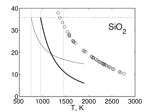
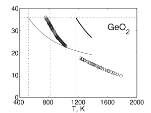
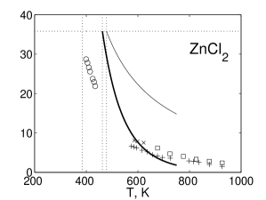
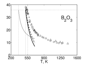
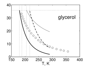
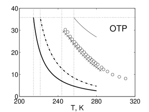
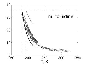
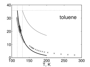
Figure 1: The free energy barrier for $\alpha$-relaxation (divided by $k_{B}T$) as a function of temperature calculated using the calorimetric bead count. The XW approximation is shown with the thin solid line and RL approximation with thick lines, see the main text for detailed explanation. The symbols correspond to experimental data; different symbols denote dinstinct experiments.

Comparison of Eqs. (8) with Eqs. (9) and (10) indicates that the RL approximation for the mismatch penalty implies there is an additional source of temperature dependence of the activation barrier, from Eq. (2), compared with the purely entropic result from the XW hard sphere-based approximation for $\sigma_{0}$. We compare the predictions of the two approximations for the barrier with experimental log-relaxation times in Fig. 1, for eight specific substances, for which all of the relevant input data are available: SiO₂, GeO₂, ZnCl₂, B₂O₃, glycerol, OTP, $m$-toluidine and toluene. The input data include the temperature dependences of the configurational entropy, elastic constants, and density. Smooth fitting curves to experimentally determined temperature dependences of the configurational entropy $s_{c}^{(m)}$ (and the corresponding heat capacity) per stoichiometric unit, for all eight substances under consideration, have been kindly provided to us by Drs. Zamponi and Capaccioli. These fits were used by Capaccioli, Ruocco, and ZamponiCapaccioli et al. (2008) to estimate the complexity $s_{c}(\xi/a)^{3}$ of a rearranging region. Quantifying the complexity is of special interest in the present context since it turns out to be a universal function of the relaxation time in either RFOT-based result; we will return to it later in the article.

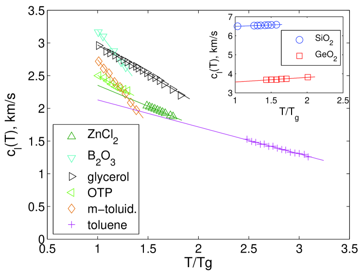
Figure 10: Temperature dependences of the longitudinal sound speed. The data for two substances are shown separately in the inset because of their greater magnitude compared to the rest of the substances.

We remind the reader that only the configurational entropy per bead is needed to produce the predictions based on the XW approximation, while the RL approximation needs structural and elastic input too. The experimentally determined input parameters and/or references to the original papers measuring them, in the case of temperature-dependent quantities, are given in Table 1. The substances are listed in the Tables in the order of increasing of the fragility index $m$, as experimentally determined. The bead counts from calorimetry $N_{b}$ and the corresponding bead sizes $a$ are provided in Tables 2 and 3 together with other calculated quantities that are predicted by the analysis. Note in several instances, we needed to extrapolate the elastic constants and calorimetric data to outside of the temperature interval where these input data were available. The extrapolations for the elastic data are shown in Fig. 10 below, while those for the configurational entropy are provided in the Supporting Information; the latter also contains the fitting coefficients for both the elastic constants and entropy.

In Fig. 1, the symbols indicate the experimental values of the free energy barrier (divided by $k_{B}T$), obtained from the measured relaxation times. For the latter, we used data compiled by Capaccioli, Ruocco, and ZamponiCapaccioli et al. (2008), and other sources, see the Supporting Information for details. For this determination, the high-$T$ limit of the relaxation time is taken to be $\tau_{0}=1$ ps: $F^{\ddagger}/k_{B}T=\ln(\tau/\tau_{0})$. In reality, although the high-$T$ value of $\tau$ is usually in the vicinity of a picosecond, as determined by the vibrational relaxation time, system-specific deviations from the latter value may be present. Consequently, for each order of magnitude worth of such deviation, the experimental points on Fig. 1 would be off by $\ln 10\approx 2.3$. The thin solid line shows the free energy barrier computed with Eq. (2) using the XW prediction (8) for $\sigma_{0}$.

The thick lines in Fig. 1 show the barrier (divided by temperature) computed using the RL prediction for $\sigma_{0}$, Eqs. (9) and (10). Some of the substances fall into the regime corresponding to just one of these equations in the full temperature range. In such cases, the corresponding equation number is provided in Table 1. Some substances obey Eq. (9) at low $T$ but make a change, at some temperature above $T_{g}$, to the regime in which the uniform liquid states are bypassed during reconfigurations so that Eq. (10) now applies. Under these circumstances, we provide, in Table 1, the temperature of that change.

The graph for B₂O₃ contains a thick dashed line, which accounts for the temperature dependence of its bead size. This matter has been discussed extensively by two of us in Ref.Rabochiy and Lubchenko (2012b) and has to do with a gradual ordering transition in B₂O₃, in which the rigid molecular units at sufficiently high temperatures can be thought of as BO₃ triangles, but at low temperatures they are essentially the boroxol rings B₃O₆.

Last, but not least, all of the RL-based calculations mentioned so far employ a temperature independent structure $S(k)$ measured near $T_{g}$. Unfortunately, there is a lack of data at other temperatures (see Table 1 for the specific temperature $T_{S}$ at which $S(k)$ was measured for each substance). For two of the liquids, i.e., glycerol and OTP, we have also found $S(k)$’s measured at an additional, higher temperature, see Table 1. We present the barrier values computed using the $S(k)$ measured at these high temperatures as the dashed-dotted lines. We observe that the computed barrier values, at high temperatures, move in the right direction and, in the case of glycerol, almost coincide with the measured value at the higher temperature at which $S(k)$ is known, i.e., 295 K. This notion suggests that accounting for the temperature dependence of the structural factor may be in fact important for quantitative barrier estimates. Finally, we have not found $S(k)$ for toluene measured at $T_{g}$, but only at a higher temperature and higher pressure, which should be a reasonable substitute for the $S(k)$ at $T_{g}$, as two of us argued elsewhereRabochiy and Lubchenko (2013).

	$M$, $10^{-25}$kg	$T_{S}$, K	$T_{m}$, K	$\Delta H$, kJ/mol	$c_{l}$	$\rho$	Eq.	Eq.(sc)
SiO2Mei et al. (2008)	1.00	1452	1995	9.60	Polian et al. (2002)	Levelut et al. (2005)	(10)	(9)
GeO2Salmon et al. (2007)	1.74	816	1389	17.1	Youngman et al. (1997)	Dingwell et al. (1993)	(9)	(9)
ZnCl2Zeidler et al. (2010)	2.26	385	598	10.3	Dreyfus et al. (2001)	Gruber and Litovitz (1964)	(9)	$T_{c}=418$ K
B2O3Swenson et al. (1995)	1.16	553	723	24.6	Grimsditch et al. (1989)	Macedo et al. (1966)	(9)	(9)
glycerolHanely et al. (1987)	1.53	183, 295	291	18.3	Kovalenko et al. (2009); Comez et al. (2003)	Scarponi et al. (2004)	(10)	(10)
OTPBartsch et al. (1993)	3.82	255, 314	329	17.2	Dreyfus et al. (2003); Monaco et al. (2001)	Monaco et al. (2001)	(10)	(10)
m-toluid.Alba-Simionesco et al. (1998)	1.78	210	242	8.80	Dreyfus et al. (2002)	Aouadi et al. (2000)	$T_{c}=210$ K	$T_{c}=212$ K
tolueneAlba-Simionesco et al. (1998)	1.53	293*	178	6.64	Rubio et al. (2001)	Rubio et al. (2001)	$T_{c}=134$ K	$T_{c}=135$ K

Table 1: The melting temperature $T_{m}$ is obtained from Ref.CRC (2011) for all substances; the fragility index $m$, glass transition temperature $T_{g}$, heat of fusion $\Delta H$ and heat capacity jump $\Delta C_{p}$ at $T_{g}$ are from Ref.Wang et al. (2006) for all substances except SiO₂, Refs.Böhmer et al. (1993); CRC (2011); Sipp et al. (2001). The quantity $T_{S}$ is the temperature at which the structure factor $S(k)$ is known. The asterisk at toluene’s $T_{S}$ indicates the structure factor is known at a higher pressure, see text. $c_{l}$ and $\rho$ stand for the longitudinal sound speed and density respectively. The last two columns indicate whether Eq. (9) and (10) was used to calculate the surface tension in the RL approach. If both equations have been used—Eq. (9) at lower $T$ and Eq. (10) at higher $T$— we indicate the temperature $T_{c}$ that separates the two regimes.

	$a$, Å	$a^{\text{sc}}$, Å	$N_{b}$	$N_{b}^{\text{sc}}$	$m_{\text{exp}}$	$m_{\text{th}}$	$m_{\text{th}}^{\text{sc}}$	$T_{g}^{\text{exp}}$, K	$T_{g}^{\text{th}}$, K	$\xi_{\text{exp}}$, nm	$\xi_{\text{th}}$, nm
SiO2	5.09	4.49	0.34	0.50	20	47	35	1452	958	2.91	2.42
GeO2	3.79	4.37	0.88	0.57	20	27	30	816	1168	1.93	1.73
ZnCl2	4.13	4.64	1.23	0.87	30	82	94	385	462	2.27	2.33
B2O3	3.33	3.13	1.58	1.81	36	68	76	553	506	1.06	1.40
glycerol	2.95	2.89	4.50	4.82	53	108	103	188	179	0.82	1.85
OTP	4.50	3.44	3.74	8.41	81	355	134	244	214	1.60	3.91
m-toluid.	3.99	3.90	2.60	2.79	98	174	160	185	182	1.61	2.44
toluene	3.82	3.79	2.67	2.73	103	137	139	116	116	1.60	2.46

Table 2: The quantities $a$, $N_{b}$, $m$, and $T_{g}$ stand for the bead size, bead count, fragility index, and glass transition temperature respectively. The index “th” signifies the quantity was computed using the Rabochiy-Lubchenko (RL) approximation. The index “sc” signifies the corresponding quantities were evaluated using the “self-consistent” procedure for determining the bead count explained in the text.

	$a$, Å	$a^{\text{sc}}$, Å	$N_{b}$	$N_{b}^{\text{sc}}$	$m_{\text{exp}}$	$m_{\text{th}}$	$m_{\text{th}}^{\text{sc}}$	$T_{g}^{\text{exp}}$, K	$T_{g}^{\text{th}}$, K	$\xi_{\text{exp}}$, nm	$\xi_{\text{th}}$, nm
SiO2	5.09	3.98	0.34	0.72	20	37	9	1452	755	2.91	2.76
GeO2	3.79	3.42	0.88	1.20	20	11	11	816	521	1.93	2.04
ZnCl2	4.13	4.98	1.23	0.70	30	26	47	385	478	2.27	2.25
B2O3	3.33	2.51	1.58	3.53	36	55	16	553	359	1.06	1.76
glycerol	2.95	3.20	4.50	3.53	53	39	49	188	205	0.82	1.60
OTP	4.50	4.86	3.74	2.97	81	61	79	244	256	1.60	2.47
m-toluid.	3.99	4.38	2.60	1.97	98	71	95	185	194	1.61	2.17
toluene	3.82	4.48	2.67	1.65	103	50	98	116	131	1.60	2.08

Table 3: The quantities $a$, $N_{b}$, $m$, and $T_{g}$ stand for the bead size, bead count, fragility index, and glass transition temperature respectively. The index “th” signifies the quantity was computed using the Xia-Wolynes (XW) approximation. The index “sc” signifies the corresponding quantities were evaluated using the “self-consistent” procedure for determining the bead count explained in the text.

We observe that for most of the substances the agreement between the experiment and the theoretical predictions does leave some room for improvement. However, given that no adjustable parameters were used, the agreement seems satisfactory, considering the input data are purely static. To put things in perspective, we note that we are unaware of any existing calculation that starts from the corresponding information such as (high-frequency) elastic constants and structure factor of a liquid and produces a figure for the crystal-nucleation barrier with an accuracy comparable to that seen in Fig. 1. At any rate, we feel the present degree of agreement would justify further studies that include more substances and suggests that the present approximations provide a reasonable formal basis for further systematic improvement.

Let us list possible errors that may arise in applying the present formalisms to specific substances. Both RFOT based expressions for the absolute barrier rely on accurate estimates of the bead size, by Eqs. (8-10), (16). As discussed elsewhereZhugayevych and Lubchenko (2010), the calorimetric bead count is especially likely to be off when local ordering is present, as in chalcogenide alloysZhugayevych and Lubchenko (2010) or the aforementioned boron oxideRabochiy and Lubchenko (2012b). To get a sense of the issue, consider the fusion entropy for chalcogenides. Almost independent of the stoichiometry, the fusion entropy in these materials is about $1.5k_{B}$ per atom—a typical value for ionic compoundsCRC (2011)—suggesting there is roughly one bead per atom. Yet it is clear that in As₂Se₃, for instance, the AsSe₃ pyramids are deformed little during liquid motions, implying instead a bead per arsenic atomZhugayevych and Lubchenko (2010). Now, the RL calculation is quite sensitive to the precise value of the structure factor. As discussed in detail in Ref.Rabochiy and Lubchenko (2013), the latter is subject to significant experimental uncertainty for the relatively small values of $k$ in question. Last but not least, the RL formula relies on accurate measurement of the elastic constants, which becomes progressively more difficult at increasing temperatures especially because of the problem of separating the purely elastic from the relaxational part of the stress response.

From the theoretical vantage point, we point out that neither the XW nor RL formulas completely contains all known effects that have been previously considered within the RFOT theory. Specifically, neglected are the barrier softening effects that arise from approaching the mode coupling temperatureLubchenko and Wolynes (2003). The latter effects stem from the spatial variation in the order parameter in the critical droplet near the crossover; the resulting transition rate between distinct aperiodic states is faster than what the simple nucleation-like argument predicts. The XW expression ignores the softening altogether. It would predict a finite nucleation rate even above the mean field dynamical transitionLubchenko and Wolynes (2003). The RL expression does exhibit some degree of softening since it employs empirically determined elastic constants. The RL approach nevertheless disregards several aspects of the instanton structure including the limited applicability of the renormalized surface tension coefficient in Eq. (1) close to the crossoverLubchenko and Wolynes (2003). Indeed, contrary to the assumptions behind Eq. (1), the reconfigurations are accompanied by string-like excitations close to $T_{\mbox{\scriptsize cr}}$ implying, among other things, that the interface is not thinStevenson et al. (2006).

A potential concern specific to the XW estimate for $\sigma_{0}$ is that it should be most accurate near $T_{K}$, as already mentioned. One of the sources of ambiguity in the RL approach, on the other hand, is the simplifying assumption on the vibrational spectrum, which was assumed to be Debye-like with a sharp cutoff at $k=\pi/a$. In reality, the cut-off should be soft; the $S^{\prime}(k)$ derivative would be replaced by a more complicated, integral expression under these circumstances, thus requiring the knowledge of $S(k)$ at even lower values of $k$. Finally, there is potential error in how one converts from the atomic to the bead-wise structure factor.

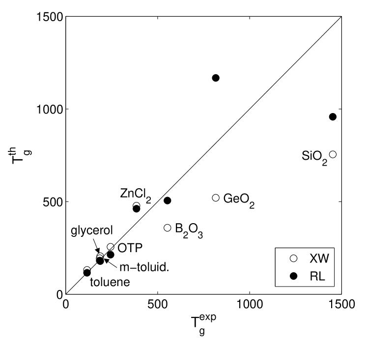
Figure 2: Theoretically predicted glass transition temperatures $T_{g}$, calculated using the XW and RL approximations for the mismatch penalty, plotted against experimental values. The theoretical temperatures are based on the barriers from Fig. 1 which rely on static input data, while the experimental values are kinetic quantities obtained from calorimetry.

It is instructive to provide a partial summary of the data in Fig. 1 by plotting the glass transition temperatures, as predicted by the theory, against their experimental values (they are also tabulated in Tables 2 and 3 for the RL and XW-based estimates respectively). For the sake of argument, we assume the time scale of the glass transition is $\tau_{g}=1$hr, while the vibrational relaxation time $\tau_{0}=10^{-12}$ sec. By Eq. (7), this implies $F^{\ddagger}(T_{g})/T_{g}=\ln(3.6\cdot 10^{15})\approx 35.8$. Fig. 2 shows the result of the calculation. We observe that the predicted glass transition temperatures agree well with the experimental values, despite the sometimes large discrepancy between theory and experiment for the rates themselves in Fig. 1. Note that in Fig. 2 and the Tables we use the experimental $T_{g}$ as determined calorimetrically, instead of using relaxation data, and so one should expect some discrepancy between the relaxation time-based apparent $T_{g}$, as inferred from Fig. 1, and the calorimetric $T_{g}$, which is indicated by a vertical line on the same figure. This discrepancy is generally present because of variations in the quench rate, sample purity, detailed fitting of the DSC curve, etc.

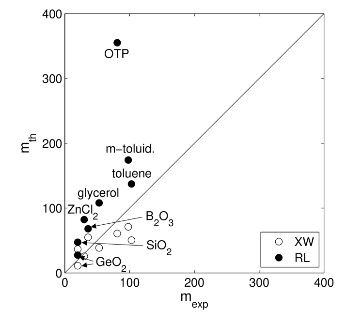
Figure 3: The fragility indices for several substances, Eq. (5), corresponding to the barriers from Fig. 1 plotted against their experimental values.

Incidentally, one can compute the slopes of the curves from Fig. 1 at the glass transition temperature, in the form of fragility indices, see Eq. (5). We emphasize that the theoretically predicted fragility indices shown in the Tables were computed at the predicted $T_{g}$, not at the experimental glass transition temperature. Fig. 3 shows this measure of liquid fragility plotted against its experimental value, for the eight substances in question. We note that both the RL and XW approximation show a good correlation with measurement, except for the RL prediction for OTP, to be commented on shortly.

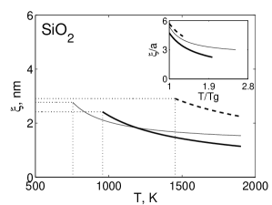
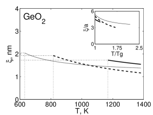
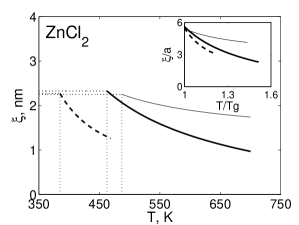
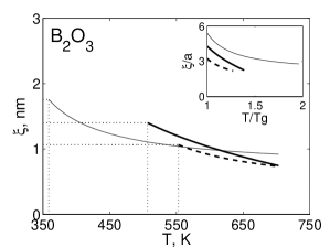
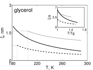
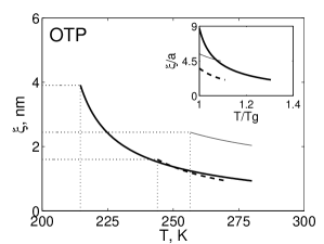
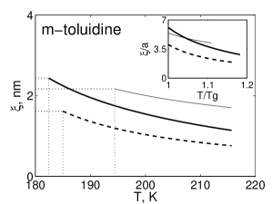
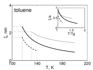
Figure 4: Comparison of the RFOT-based predictions for the cooperativity length $\xi$ as a function of temperature from Eq. (3) (solid lines) with the “experimental” cooperativity length (dashed line) determined according to the procedure by Berthier et al.Berthier et al. (2005), see Eq. (18). The thick and thin solid lines correspond to the RL and XW approximation for the mismatch penalty respectively. The vertical dotted lines indicate the respective glass transition temperatures for each set of data, as in Fig. 1. The horisontal dotted lines are added as a visual aid. The insets are lengths scaled by the bead size and refer to temperature scaled by the respective glass transition temperatures.

Next, in Fig. 4, we show the temperature dependence of the cooperativity length $\xi$ from Eq. (3). The thin and thick solid lines show the result of the XW and RL based calculations respectively. The respective temperature intervals for the RL and XW lengths correspond to the temperature intervals in Fig. 1; they do not coincide because the predicted glass transition temperatures are different for the two approximations. Now, the dashed line shows the dynamical correlation length $\xi$ computed according to the procedure of Berthier et al.Berthier et al. (2005):

$$\xi/a=\left\{\frac{1}{\pi}\left[\frac{\beta}{e}\frac{\partial\ln\tau}{\partial\ln T}\right]^{2}\frac{k_{B}}{\Delta c_{p}}\right\}^{1/3},$$ (18)

where $\beta$ is the exponent in the stretched exponential relaxation profile: $e^{-(t/\tau)^{\beta}}$. As already mentioned, we have used the calorimetric data of Capaccioli, Ruocco, and ZamponiCapaccioli et al. (2008). In addition we have used their fitting forms for the relaxation times and, when available, the stretching exponent $\beta$. The corresponding fits are shown in the Supporting Information. For three of the substances—glycerol, ZnCl₂, and B₂O₃—the temperature dependence of $\beta$ was available, while for the rest of the substances, a constant value for this quantity, as measured near $T_{g}$, was adopted for the lack of data for $\beta$ in the extended temperature range just as was done by Capaccioli et al.Capaccioli et al. (2008) previously. Berthier et al. have argued that although the $\xi$ from Eq. (18) is a lower bound, it should be numerically close to the actual value of the cooperativity length. One may thus regard this quantity as an experimentally inferred dynamical correlation length. Fig. 4 demonstrates that both the XW and RL determined lengths are generically quite close to the experimental $\xi$. Deviations, when present, echo those for the computed barriers in Fig. 1. This is expected based on Eqs. (2) and (3). Finally, the insets in Fig. 4 show the same lengths as the main graphs, but normalized by $a$ and as functions of temperature normalized by the respective $T_{g}$, to simplify comparison.

To see whether an error in the absolute barrier values above is potentially due to incorrectly determined bead size, we perform a procedure analogous to what RL did to assess the effects of bead size on their $\sigma_{0}$ values. This procedure gave a bead size that was chemically reasonable (as in the As₂Se₃ example), except for OTPRabochiy and Lubchenko (2013), where the self-consistent bead count is too high. (This issue was pointed out previously by Rabochiy and LubchenkoRabochiy and Lubchenko (2013) and may be related to uncertainty in the experimental structure factor.) Likewise, we can rescale the bead size by a constant factor so that the hereby computed barrier values match experiment at the glass transition temperature itself. This is particularly straightforward in the XW case, where the barrier is proportional to the bead count $N_{b}$, and so the barrier is rescaled simply by a constant factor. It is more cumbersome to do this, but not too much so, for the more complicated RL expressions, where (numerically) solving a non-linear equation is required. We will call this way of fixing the bead size, i.e., based on a predetermined value of the absolute free energy barrier at $T_{g}$, the “self-consistent” bead count. As in Fig. 2, we fix $F^{\ddagger}(T_{g})/T_{g}=\ln(3.6\cdot 10^{15})\approx 35.8$. The bead counts obtained in this way and the corresponding bead sizes are listed in Tables 2 and 3.

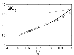
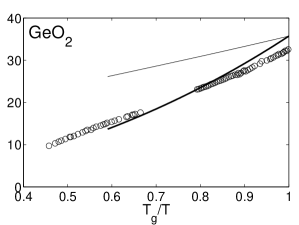
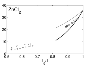
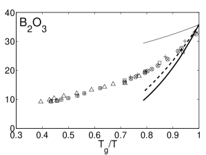
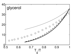
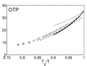
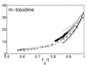
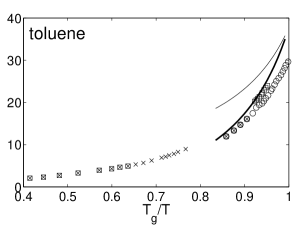
Figure 5: Barrier for $\alpha$-relaxation (divided by $k_{B}T$) as a function of temperature calculated using the self-consistent bead count. The XW approximation is shown with the thin solid line and RL approximation with thick lines, see the main text for detailed explanation. In all graphs, the temperature is scaled by the experimentally determined $T_{g}$.

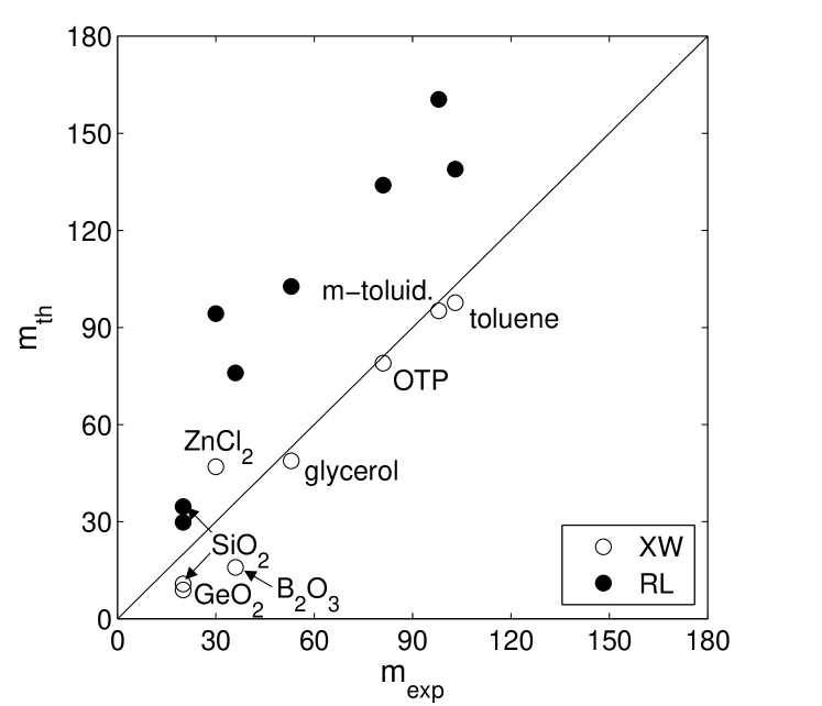
Figure 6: The fragility indices, Eq. (5), corresponding to the activation barriers from Fig. 5, computed using the self-consistently determined bead count, plotted against experimental values.

In Fig. 5, we present the temperature-dependent barrier values computed when the self-consistent bead count is employed. Neither the high temperature relaxation time $\tau_{0}$ nor the time scale of the glass transition for the experimental systems in question is available, and so some discrepancy between theory and experiment is built-in at the onset. This amounts to only a mild inconvenience, however, as the reader can infer from Fig. 5. The latter figure lets one focus on the slope of the temperature dependence of the barriers, as opposed to their absolute values. The legend in this figure is the same as in Fig. 1. Now, the fragility indices corresponding to Fig. 5 are shown in Fig. 6, to be compared with those in Fig. 3. We observe that both the RL-based and XW-based values of the fragility index show a better correlation with experiment than for the calorimetrically determined bead count. For both ways to count beads, the RL-based prediction consistently overestimates the rate of the barrier decrease with temperature. Note that the because of the rescaling, the effect of using a different structure factor for glycerol and OPT is quite small.

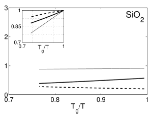
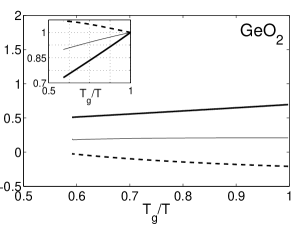
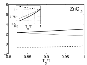
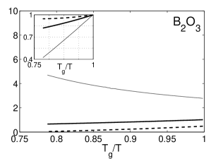
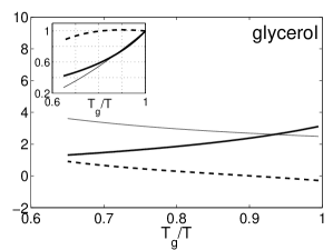
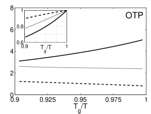
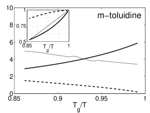
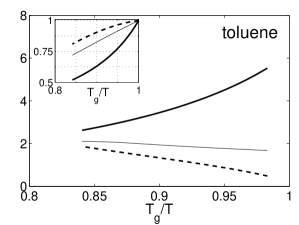
Figure 7: The logarithmic temperature derivative, $(\partial/\partial\ln T)\ln$, of the entropic (thick solid line) and the remaining contribution (thin solid line) to the RL-based barrier $F^{\ddagger}$. The thick dashed line corresponds to $F^{\ddagger}_{\text{exp}}s_{c}$, where $F^{\ddagger}_{\text{exp}}$ is the experimentally determined barrier; this would be the actual non-entropic contribution to the barrier change according to Eq. (1). Insets: the entropic contribution ( thin line) and remaining contribution (thick line) to the RL-based barrier as functions of temperature, normalized to 1 at $T_{g}$. In both main graph and inset, we use the calorimetric bead count.

According to Figs. 5 and 6, the XW approximation consistently yields an adequate estimate for the rate of change of the barrier with temperature, near the glass transition as defined by a fixed free energy barrier. At the same time, it systematically underestimates this variation at higher temperatures. This agrees with our earlier remarks on the progressively more dominant contribution of the configurational entropy to the temperature variation the closer one is to $T_{K}$. The RL argument suggests that some of the missing portion of the temperature dependence in XW formulation is, in fact, due to the temperature dependence of the elastic constants. Apart from the overall magnitude of the barrier, the RL-predicted rates of change of the barrier with temperature seem to be closer to experiment in the broader temperature range, even though they are now overestimated. We will comment on the latter in the Discussion Section. For now, it seems instructive to assess the relative contributions of the configurational entropy, $1/s_{c}(T)$, and the elastic constants, $F^{\ddagger}_{\text{RL}}(T)s_{c}(T)$, to the temperature dependence of the RL-based value of the barrier $F^{\ddagger}$. Note that because we use a constant value of the structure factor $S(k)$, the latter does not contribute to the temperature dependence of the barrier. Now, the main panels of Fig. 7 show the logarithmic derivatives of the logarithm of the entropic and elastic contributions, which allows one to compare the corresponding rates of change of these quantities not only for each given substance separately but also across different substances. Here, the thick solid line depicts the entropic part. The thin solid line corresponds to the RL prediction of the elastic contribution alone, i.e, $F^{\ddagger}_{\text{RL}}(T)s_{c}(T)$. The thick dashed line corresponds to the elastic contribution as assessed on the experimentally determined value of the barrier, i.e, $F^{\ddagger}_{\text{exp}}(T)s_{c}(T)$; this would be the actual non-entropic contribution to the barrier change according to Eq. (1). We observe that the “experimentally inferred” elastic contribution to the temperature dependence of the barrier is consistently lower than the contribution from the variation of the entropy. In some cases, the so determined elastic variation is in fact negative, which may well be due to uncertainties in the experimental inputs. The situation with the RL-based microscopic prediction of the elastic contribution is a bit more complicated. In two cases, it exceeds the entropic contribution, while in the other cases it is comparable or less than the latter. In all cases, however, the configurational entropy becomes more important as $T_{g}$ is approached. As to the inconsistency of the RL estimate, compared with the experiment-based estimate, we suggest that our ignoring the temperature dependence of the structure factor may be to blame. At any rate, note that since the RL barrier overestimates the fragility, the effect of the RL-based temperature dependence of the elastic constants, as shown in Fig. 7, is probably overestimated, too.

The above assessment of the relative contributions of the configurational entropy and the elastic constants to the temperature dependence of the barrier relies, of course, on the RFOT-based expression (2). One can actually test the internal consistency of the latter RFOT expression in a manner that is independent of the value of the surface tension $\sigma_{0}$, and thus is in no way affected by the temperature dependence of the elastic constants, among other things. There is a simple relationship between the $\alpha$-relaxation barrier (or, equivalently, $\ln(\tau/\tau_{0})$) and the product $(\xi/a)^{3}s_{c}/k_{B}$, which is often called the “complexity” of the rearranging region. Indeed, dividing Eq. (2) by (3), one obtains that the complexity of a rearranging region is simply the barrier, in units of $k_{B}T$, times a factor of four:

$$(\xi/a)^{3}s_{c}/k_{B}=4F^{\ddagger}/k_{B}T=4\ln(\tau/\tau_{0})$$ (19)

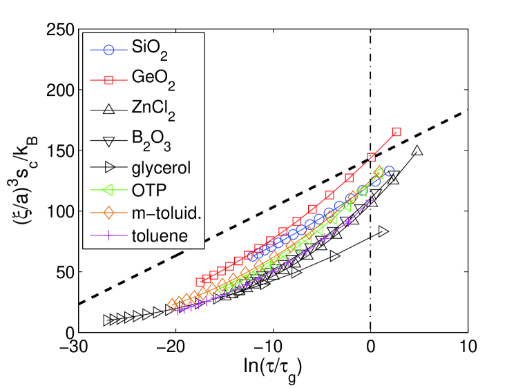
Figure 8: The experimentally inferred complexity of a rearranging region $s_{c}(\xi/a)^{3}$ is plotted (symbols) as a function of $\ln(\tau/\tau_{g})$, where $\tau_{g}$ is the relaxation time $\tau$ at $T_{g}$. The cooperativity length $\xi$ in this graph is estimated as in Ref.Capaccioli et al. (2008). The dashed lines line corresponds to the universal prediction from either form of the RFOT theory. This result does not depend on substance.

This relationship can be interpreted as saying rearrangement involves searching through all the states of a fixed fraction of the rearranging regionWolynes (1997). The relationship in Eq. (19) was tested by Capaccioli, Ruocco, and ZamponiCapaccioli et al. (2008) for a large number of actual substances. For the present purposes, it is convenient to plot the complexity as a function of $\ln(\tau/\tau_{g})$, where $\tau_{g}\equiv\tau(T_{g})$. In Fig. 8 we thus plot the complexity as a function of $\ln(\tau/\tau_{g})$ for the (experimentally determined) cooperativity lengths $\xi$ computed according to Eq. (18) and shown earlier in Fig. 4 as the dashed lines. The agreement of the “experimentally” determined complexity with the RFOT-based prediction from Eq. (19) is good. For one thing, the magnitudes are nearly universal and quite consistent. The functional dependence in Fig. 8 is approximately the straight line predicted by Eq. (19), however consistently there appears to be upward curvature. This is not entirely unexpected in view of the aforementioned softening effects, which are not accounted for in Eq. (19), as well as mode-coupling effectsBhattacharyya et al. (2008).

Still, it seems instructive to assess the potential ambiguity stemming from our neglect of the temperature dependence of the stretching exponent $\beta$ when computing $\xi$ for five of the substances. Such ambiguity is expected to be especially significant for fragile substancesXia and Wolynes (2001). In the absence of experimental data, we can utilize the expression for the temperature dependence of $\beta$ derived by Xia and WolynesXia and Wolynes (2001), based on their approximation for the barrier distribution and later modified slightly by LubchenkoLubchenko (2007) to achieve a better consistency between the distribution and experimental dielectric spectra:

$$\beta_{\text{XWL}}=\left[1+\left(\frac{F/k_{B}T}{8\sqrt{D}}\right)^{2}\right]^{-1/2},$$ (20)

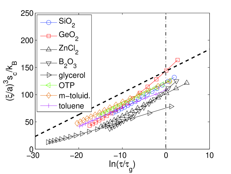
Figure 9: The complexity of a rearranging region $s_{c}(\xi/a)^{3}$ is plotted as a function of $\ln(\tau/\tau_{g})$, where $\tau_{g}$ is the relaxation time $\tau$ at $T_{g}$. The cooperativity length $\xi$ in this graph is estimated as in Ref.Capaccioli et al. (2008), except here we use the Xia-Wolynes-Lubchenko expression for the temperature dependence of the stretching exponent $\beta$ normalized so that it matches its experimental value at $T_{g}$.

where $D$ is the fragility as defined by the Vogel-Fulcher fitting form: $\tau=\tau_{0}e^{DT_{K}/(T-T_{K})}$. We plot, in Fig. 9, the complexity values computed using the XWL-based estimate of the temperature dependence of $\beta$ while normalizing the $\beta(T)$’s so that their value at $T_{g}$ matches the experimental values as before. For the sake of argument, we employed the latter procedure for all eight substances including those three for which an experimentally determined $\beta(T)$ is available. We see utilizing a reasonable estimate for the temperature dependence of the non-exponentiality removes much of the curvature. Clearly better measurements of $\beta(T)$ are needed before strict values of the scaling exponents can be assigned.

IV Discussion

We have presented calculations of the absolute free energy activation barriers for $\alpha$-relaxation in supercooled liquids over a finite temperature range from two microscopic but approximate theories both based on RFOT ideas. We used thermodynamic, static structural, and elastic inputs solely and no adjustable parameters. Both calculations are based on the RFOT theoryKirkpatrick et al. (1989); Xia and Wolynes (2000); Lubchenko and Wolynes (2004), by which the molecules move as a result of mutual nucleation of distinct aperiodic free energy minima; the corresponding activation energy profile is given by Eq. (1). Two different estimates for the mismatch penalty $\sigma_{0}$, due to Xia and WolynesXia and Wolynes (2000) and Rabochiy and LubchenkoRabochiy and Lubchenko (2013) have been employed and compared with each other and measured kinetic data. Among its other weaknesses, the XW estimate disregards potential effects of any temperature dependence of the elastic constants. On the other hand, it is rather general, even if approximate, relatively simple, and requires only thermodynamic input information. The RL estimate, on the other hand, explicitly accounts for details of structure and bonding in liquids. It is however rather intricate and in its current form uses additional measured static quantities as input.

In comparing with experiment, the XW formulation appears robustly to determine the values of the barrier and fragility index near $T_{g}$, while the RL approach seems to better capture the temperature dependence over a more extended temperature range. The better performance of the XW approximation near $T_{g}$ is perhaps to be expected for deep reasons since the elastic effects must saturate at very low $T$ so long as no new phase transitions occur; hereby the dramatic barrier growth at lowering temperatures is more dominated by the configurational entropy decrease, the lower the temperature. The latter notion is indeed explicitly confirmed by our calculation, see Fig. 7.

The present results also indicate that first principles estimates of the glass transition temperature itself for real substances are in sight. Indeed, given a known value of the configuration entropy, as a function of temperature, one can use Eq. (1), and Eqs. (8) or (9-10) to estimate the temperature dependence of the barrier. To a specific value of the latter, there corresponds a glass transition on the respective time scale. Here, we have demonstrated this notion by using the experimentally determined configurational entropy. Note that RFOT-based estimates of temperature scales are robust even when no other temperature scales are explicitly used in the calculation. For instance, Rabochiy and Lubchenko have recently estimated the crossover temperature $T_{\mbox{\scriptsize cr}}$ for several substancesRabochiy and Lubchenko (2012b), which all turned out to be consistently above the glass transition temperature.

We have already mentioned that the entropy variation is the major contributor to the barrier growth at low temperatures. Yet the temperature dependence of factors other than the entropy, such as the local structure, seems to be important for truly quantitative estimates. In the RL formalism, the force details enter through the elastic constants and the coordination, via the structure factor $S(k)$. Under certain circumstances, the barrier scales linearly with the elastic constants, which hearkens back to earlier, enthalpy based approaches to activated dynamics by Hall and WolynesHall and Wolynes (1987) and the so called “shoving model”Dyre et al. (1996). Note, however, that in the RL formulation there is also another significant contribution to the mismatch energy cost, contained in the curly brackets in Eq. (9). Now, the shoving model, in some of its particular realizationsDyre and Wang (2012); Klieber et al. (2013), proposes that the activation barrier grows exclusively because of the increase in the elastic constants at the “plateau” frequencies. In contrast, the RL approach would seem to call for high frequency elastic constants, as being the relevant ones for vibrational motions of individual beads. Also importantly, the RL approach calls not for the shear modulus alone, but the longitudinal sound speed, which amounts to a combination $K+4\mu/3$ of the bulk modulus $K$ and shear modulus $\mu$. As far as these high frequency moduli are concerned, we have seen in Fig. 7 that their temperature dependence is, in fact, important for quantitative estimates of the barrier over an extended temperature range. Still, it is essential to develop a formal theory with regard to the latter effects, which, generally, leads to complicated expressions as in Eq. (9). If one were simply to look for direct correlation between the elastic constants and the barrier, one would discover that this correlation is complicated, if any. For instance, in SiO₂ and GeO₂, the measured elastic constants increase with temperature, i.e., change in the direction opposite to the barrier change, as we show in Fig. 10.

In further discussing the relative importance of the entropic vs. elastic contributions to the barrier growth, we note that the entropic contribution entirely, quantitatively accounts for the discrete change in the apparent activation energy at the glass transitionLubchenko and Wolynes (2003). As a result the change is directly correlated with the heat capacity jump, and, hence, with the fragilityXia and Wolynes (2000); Lubchenko and Wolynes (2003); Stevenson and Wolynes (2005). A purely elasticity-based theory would also predict a jump, if the elastic constants measured at the plateau show a discontinuity in slope, at $T_{g}$, in their temperature dependences. (High-frequency constants certainly do so.) It thus seems important to investigate whether the measured discontinuity of the elastic constants would in fact correlate with the fragility of the liquid.

The present methodology relies on the inherent relationship between thermodynamics (the configurational entropy) and kinetics (the activation barrier for liquid rearrangement), which has been constructively derived within the RFOT framework, see Eq. (2). This deep relationship is reflected in a simple, RFOT-based prediction of a relation between the complexity of a rearranging region and the relaxation time, Eq. (19). This relation is universal in that it does not depend on the value of the mismatch penalty between distinct aperiodic free energy minima, which may indeed be temperature dependent; it is therefore not subject to various uncertainties stemming from input experimental data or approximations needed to estimate the mismatch penalty. The complexity also does not depend on the notion of spherical subunits, i.e., “beads”. We have found that the RFOT-derived, universal expression (19) is indeed consistent with observation. It is worth remarking that although the increase of the complexity of a rearranging region with relaxation time scale is a robust prediction of both incarnations of the RFOT theory, it is decidedly not expected in other pictures. Adam and Gibbs argued for an increase in the size of the correlated region on cooling; their argument was, however, precisely based on the assumption of a fixed limiting complexity of a rearranging region. This is clearly contradicted by the data when the Berthier analysis is used: The complexity changes at least by a factor of three over the temperature interval in question. In enthalpically-based versions of pure elastic models the rearrangement is assumed to have a fixed size. This assumption, combined with the experimentally established decrease of specific configurational entropy with increasing relaxation time, would yield a decreasing complexity of the rearranging region upon cooling. This is contradicted even more forcefully by the observations. The near universality of the complexity with increasing relaxation time growth, seen in the data, is, in our view, direct evidence that entropy and correlation length are intimately related. This lends further, strong support for a key non-trivial aspect of the RFOT viewpoint.

Acknowledgments: We are indebted to Matthieu Wyart for stimulating discussions of the temperature dependence of the elastic constants, which partially motivated this work. We thank Francesco Zamponi and Simone Capaccioli for sharing fits of the experimental data for the configurational entropy, relaxation times, and the stretching exponent $\beta$; and also Philip S. Salmon for making available $S(k)$ data for several substances. P.R. and V.L. gratefully acknowledge the support by the NSF Grant CHE-0956127, the Welch Foundation Grant No. E-1765, and the Alfred P. Sloan Research Fellowship. The work of P.G.W. is supported in part by the Center for Theoretical Biological Physics sponsored by the NSF (PHY-0822283) and the D. R. Bullard-Welch Chair at Rice University.

References

- Biroli and Garrahan (2013) G. Biroli and J. P. Garrahan, J. Chem. Phys. 138, 12A301 (2013).
- Lubchenko and Wolynes (2007a) V. Lubchenko and P. G. Wolynes, Annu. Rev. Phys. Chem. 58, 235 (2007a).
- Kirkpatrick et al. (1989) T. R. Kirkpatrick, D. Thirumalai, and P. G. Wolynes, Phys. Rev. A 40, 1045 (1989).
- Xia and Wolynes (2000) X. Xia and P. G. Wolynes, Proc. Natl. Acad. Sci. 97, 2990 (2000).
- Villain (1985) J. Villain, J. Physique 46, 1843 (1985).
- Lubchenko and Wolynes (2003) V. Lubchenko and P. G. Wolynes, J. Chem. Phys. 119, 9088 (2003).
- Bevzenko and Lubchenko (2009) D. Bevzenko and V. Lubchenko, J. Phys. Chem. B 113, 16337 (2009).
- Lubchenko and Wolynes (2004) V. Lubchenko and P. G. Wolynes, J. Chem. Phys. 121, 2852 (2004).
- Hall and Wolynes (2008) R. W. Hall and P. G. Wolynes, J. Phys. Chem. B 112, 301 (2008).
- Mézard and Parisi (1999) M. Mézard and G. Parisi, J. Chem. Phys. 111, 1076 (1999).
- Parisi and Zamponi (2010) G. Parisi and F. Zamponi, Rev. Mod. Phys. 82, 789 (2010).
- L.-M. Martinez and Angell (2001) L.-M. Martinez and C. A. Angell, Nature 410, 663 (2001).
- Angell (1997) C. A. Angell, J. Res. Natl. Inst. Stand. Techol. 102, 171 (1997).
- Rabochiy and Lubchenko (2013) P. Rabochiy and V. Lubchenko, J. Chem. Phys. 138, 12A534 (2013).
- Stevenson and Wolynes (2005) J. Stevenson and P. G. Wolynes, J. Phys. Chem. B 109, 15093 (2005).
- Kauzmann (1948) W. Kauzmann, Chem. Rev. 43, 219 (1948).
- Stevenson and Wolynes (2011) J. D. Stevenson and P. G. Wolynes, J. Phys. Chem. A 115, 3713 (2011).
- Ashtekar et al. (2010) S. Ashtekar, G. Scott, J. Lyding, and M. Gruebele, J. Phys. Chem. Lett. 1, 1941 (2010).
- Tracht et al. (1998) U. Tracht, M. Wilhelm, A. Heuer, H. Feng, K. Schmidt-Rohr, and H. W. Spiess, Phys. Rev. Lett. 81, 2727 (1998).
- Russell and Israeloff (2000) E. V. Russell and N. E. Israeloff, Nature 408, 695 (2000).
- Cicerone and Ediger (1996) M. T. Cicerone and M. D. Ediger, J. Chem. Phys. 104, 7210 (1996).
- Berthier et al. (2005) L. Berthier, G. Biroli, J.-P. Bouchaud, L. Cipelletti, D. El Masri, D. L’Hôte, F. Ladieu, and M. Perino, Science 310, 1797 (2005).
- Lubchenko and Wolynes (2007b) V. Lubchenko and P. G. Wolynes, Adv. Chem. Phys. 136, 95 (2007b).
- Lubchenko (2012) V. Lubchenko, J. Phys. Chem. Lett. 3, 1 (2012).
- Lubchenko and Wolynes (2012) V. Lubchenko and P. G. Wolynes, “Theories of Structural Glass Dynamics: Mosaics, Jamming, and All That,” in Structural Glasses and Supercooled Liquids: Theory, Experiment, and Applications, edited by P. G. Wolynes and V. Lubchenko (John Wiley & Sons, 2012) pp. 341–379.
- Wisitsorasak and Wolynes (2012) A. Wisitsorasak and P. G. Wolynes, Proc. Natl. Acad. Sci. 109, 16068 (2012).
- Rabochiy and Lubchenko (2012a) P. Rabochiy and V. Lubchenko, J. Chem. Phys. 136, 084504 (2012a).
- Rabochiy and Lubchenko (2012b) P. Rabochiy and V. Lubchenko, J. Phys. Chem. B 116, 5729 (2012b).
- Wisitsorasak and Wolynes (2013) A. Wisitsorasak and P. G. Wolynes, ArXiv e-prints (2013), arXiv:1305.0702 [cond-mat.dis-nn] .
- Swallen et al. (2007) S. F. Swallen, K. L. Kearns, M. K. Mapes, Y. S. Kim, R. J. McMahon, M. D. Ediger, T. Wu, L. Yu, and S. Satija, Science 315, 353 (2007).
- Dawson et al. (2009) K. J. Dawson, K. L. Kearns, L. Yu, W. Steffen, and M. D. Ediger, Proc. Natl. Acad. Sci. 106, 15165 (2009).
- Stevenson and Wolynes (2008) J. D. Stevenson and P. G. Wolynes, J. Chem. Phys. 129, 234514 (2008).
- Kirkpatrick and Wolynes (1987) T. R. Kirkpatrick and P. G. Wolynes, Phys. Rev. B 36, 8552 (1987).
- Biroli and Bouchaud (2012) G. Biroli and J.-P. Bouchaud, “The Random First Order Transition Theory of Glasses: A Critical Assessment,” in Structural Glasses and Supercooled Liquids: Theory, Experiment, and Applications, edited by P. G. Wolynes and V. Lubchenko (John Wiley & Sons, 2012) pp. 341–379.
- Mari et al. (2009) R. Mari, F. Krzakala, and J. Kurchan, Phys. Rev. Lett. 103, 025701 (2009).
- Yan et al. (2013) L. Yan, G. Düring, and M. Wyart, Proc. Natl. Acad. Sci. 110, 6307 (2013).
- Dyre and Wang (2012) J. C. Dyre and W. H. Wang, J. Chem. Phys. 136, 224108 (2012).
- Klieber et al. (2013) C. Klieber, T. Hecksher, T. Pezeril, D. H. Torchinsky, J. C. Dyre, and K. A. Nelson, J. Chem. Phys. 138, 12A544 (2013).
- Lindemann (1910) F. A. Lindemann, Phys. Z. 11, 609 (1910).
- Lubchenko (2006) V. Lubchenko, J. Phys. Chem. B 110, 18779 (2006).
- Turnbull (1950) D. Turnbull, J. Appl. Phys. 21, 1022 (1950).
- Cahn and Hilliard (1958) H. W. Cahn and J. E. Hilliard, J. Chem. Phys. 28, 258 (1958).
- Dzero et al. (2009) M. Dzero, J. Schmalian, and P. G. Wolynes, Phys. Rev. B 80, 024204 (2009).
- Capaccioli et al. (2008) S. Capaccioli, G. Ruocco, and F. Zamponi, J. Phys. Chem. B 112, 10652 (2008).
- Mei et al. (2008) Q. Mei, C. J. Benmore, S. Sen, S. R. Sharma, and J. L. Yarger, Phys. Rev. B 78, 144204 (2008).
- Polian et al. (2002) A. Polian, D. Vo-Thanh, and P. Richet, Europhys. Lett. 57, 375 (2002).
- Levelut et al. (2005) C. Levelut, A. Faivre, R. Le Parc, B. Champagnon, J.-L. Hazemann, and J.-P. Simon, Phys. Rev. B 72, 224201 (2005).
- Salmon et al. (2007) P. S. Salmon, A. C. Barnes, R. A. Martin, and G. J. Cuello, J. Phys.: Condens. Matter 19, 415110 (2007).
- Youngman et al. (1997) R. Youngman, J. Kieffer, J. Bass, and L. Duffrene, J. Non-Cryst. Sol. 222, 190 (1997).
- Dingwell et al. (1993) D. B. Dingwell, R. Knochc, and S. L. Webb, Phys. Chem. Minerals 19, 445 (1993).
- Zeidler et al. (2010) A. Zeidler, P. S. Salmon, R. A. Martin, T. Usuki, P. E. Mason, G. J. Cuello, S. Kohara, and H. E. Fischer, Phys. Rev. B 82, 104208 (2010).
- Dreyfus et al. (2001) C. Dreyfus, M. J. Lebon, F. Vivicorsi, A. Aouadi, R. M. Pick, and H. Z. Cummins, Phys. Rev. E 63, 041509 (2001).
- Gruber and Litovitz (1964) G. J. Gruber and T. A. Litovitz, J. Chem. Phys. 40, 13 (1964).
- Swenson et al. (1995) J. Swenson, L. Börjesson, and W. S. Howells, Phys. Rev. B 52, 9310 (1995).
- Grimsditch et al. (1989) M. Grimsditch, R. Bhadra, and L. M. Torell, Phys. Rev. Lett. 62, 2616 (1989).
- Macedo et al. (1966) P. B. Macedo, W. Capps, and T. A. Litovitz, J. Chem. Phys. 44, 3357 (1966).
- Hanely et al. (1987) H. J. M. Hanely, G. C. Straty, C. J. Glinka, and J. B. Hayter, Mol. Phys. 62, 1165 (1987).
- Kovalenko et al. (2009) K. Kovalenko, S. Krivokhizha, and I. Chaban, JETP 108, 866 (2009).
- Comez et al. (2003) L. Comez, D. Fioretto, F. Scarponi, and G. Monaco, J. Chem. Phys. 119, 6032 (2003).
- Scarponi et al. (2004) F. Scarponi, L. Comez, D. Fioretto, and L. Palmieri, Phys. Rev. B 70, 054203 (2004).
- Bartsch et al. (1993) E. Bartsch, B. H., P. Chieux, D. A., and H. Sillescu, Chem. Phys. 169, 373 (1993).
- Dreyfus et al. (2003) C. Dreyfus, A. Aouadi, J. Gapinski, M. Matos-Lopes, W. Steffen, A. Patkowski, and R. M. Pick, Phys. Rev. E 68, 011204 (2003).
- Monaco et al. (2001) G. Monaco, D. Fioretto, L. Comez, and G. Ruocco, Phys. Rev. E 63, 061502 (2001).
- Alba-Simionesco et al. (1998) C. Alba-Simionesco, D. Morineau, B. Frick, N. Higonenq, and H. Fujimori, J. Non-Cryst. Sol. 235-237, 367 (1998).
- Dreyfus et al. (2002) C. Dreyfus, R. Gupta, B. Bonello, C. Bousquet, A. Taschin, M. Ricci, and G. Pratesi, J. Chem. Phys. 116, 7323 (2002).
- Aouadi et al. (2000) A. Aouadi, C. Dreyfus, M. Massot, R. M. Pick, T. Berger, W. Steffen, A. Patkowski, and C. Alba-Simionesco, J. Chem. Phys. 112, 9860 (2000).
- Rubio et al. (2001) J. E. F. Rubio, V. G. Baonza, M. Taravillo, J. Nunez, and M. Caceres, J. Chem. Phys. 115, 4681 (2001).
- CRC (2011) CRC Handbook of Chemistry and Physics, 91st Edition (Taylor and Francis, 2010-2011).
- Wang et al. (2006) L.-M. Wang, C. A. Angell, and R. Richert, J. Chem. Phys. 125, 074505 (2006).
- Böhmer et al. (1993) B. Böhmer, K. L. Ngai, C. A. Angell, and D. J. Plazek, J. Chem. Phys. 99, 4201 (1993).
- Sipp et al. (2001) A. Sipp, Y. Bottinga, and P. Richet, J. Non-Cryst. Sol. 288, 166 (2001).
- Zhugayevych and Lubchenko (2010) A. Zhugayevych and V. Lubchenko, J. Chem. Phys. 133, 234504 (2010).
- Stevenson et al. (2006) J. D. Stevenson, J. Schmalian, and P. G. Wolynes, Nature Physics 2, 268 (2006).
- Wolynes (1997) P. G. Wolynes, J. Res. Inst. Stand. Technol. 102, 187 (1997).
- Bhattacharyya et al. (2008) S. M. Bhattacharyya, B. Bagchi, and P. G. Wolynes, Proc. Natl. Acad. Sci. 105, 16077 (2008).
- Xia and Wolynes (2001) X. Xia and P. G. Wolynes, Phys. Rev. Lett. 86, 5526 (2001).
- Lubchenko (2007) V. Lubchenko, J. Chem. Phys. 126, 174503 (2007).
- Hall and Wolynes (1987) R. Hall and P. Wolynes, J. Chem. Phys. 86, 2943 (1987).
- Dyre et al. (1996) J. C. Dyre, N. B. Olsen, and T. Christensen, Phys. Rev. B 53, 2171 (1996).