A Macroscopic Description of a Generalized Self-Organized Criticality System: Astrophysical Applications

Abstract

We suggest a generalized definition of self-organized criticality (SOC) systems: SOC is a critical state of a nonlinear energy dissipation system that is slowly and continuously driven towards a critical value of a system-wide instability threshold, producing scale-free, fractal-diffusive, and intermittent avalanches with powerlaw-like size distributions. We develop here a macroscopic description of SOC systems that provides an equivalent description of the complex microscopic fine structure, in terms of fractal-diffusive transport (FD-SOC). Quantitative values for the size distributions of SOC parameters (length scales $L$, time scales $T$, waiting times $\Delta t$, fluxes $F$, and fluences or energies $E$) are derived from first principles, using the scale-free probability conjecture, $N(L)dL\propto L^{-d}$, for Euclidean space dimension $d$. We apply this model to astrophysical SOC systems, such as lunar craters, the asteroid belt, Saturn ring particles, magnetospheric substorms, radiation belt electrons, solar flares, stellar flares, pulsar glitches, soft gamma-ray repeaters, black-hole objects, blazars, and cosmic rays. The FD-SOC model predicts correctly the size distributions of 8 out of these 12 astrophysical phenomena, and indicates non-standard scaling laws and measurement biases for the others.

1 INTRODUCTION

Although the paradigms of self-organized criticality (SOC) systems appear to be very intuitive and self-explaining, such as the self-adjusting angle of repose in Per Bak’s sandpile (Bak et al. 1987), or the stick-slip motion of earthquakes (Gutenberg and Richer 1949), theoreticians find it hard to establish a rigorous general definition of SOC systems. Part of the problem are the subtle differences between “criticality” in fine-tuned systems that undergo percolation or phase transitions, such as the Ising model (Ising 1925), versus “self-organized criticality” systems, which do not need any fine-tuning (e.g., Christensen and Moloney 2005). A solid definition of SOC systems should (i) be able to make quantitative predictions that are testable by observations, and (ii) provide discrimination criteria between SOC and alternative transport processes occurring in complex systems (such as random walk, branching theory, network theory, percolation, aggregation, or turbulence). A mathematical definition of SOC includes “non-trivial scale invariance (with spatio-temporal correlations) in avalanching (intermittent) systems as known from ordinary critical phenomena, but with internal, self-organized rather than external tuning of a control parameter (to a non-trivial value)” (Pruessner 2012). Alternatively, we may define SOC from a more physical point of view: SOC is a critical state of a nonlinear energy dissipation system that is slowly and continuously driven towards a critical value of a system-wide instability threshold, producing scale-free, fractal-diffusive, and intermittent avalanches with powerlaw-like size distributions. This definition applies to SOC phenomena as diverse as sandpiles, earthquakes, solar flares, or stockmarket fluctuations.

The major problem is that SOC is a microscopic process in complex systems, which cannot easily be described by macroscopic equations, unlike entropy-related processes in classical thermodynamics. In order to obtain insights into SOC processes, microscopic processes in complex systems have been simulated by iterative numerical codes, such as cellular automaton models, where a single time step is quantified by a mathematical redistribution rule, which operates on a microscopic level. Such SOC models are also called slowly-driven interaction-dominated threshold (SDIDT) systems, which all share some common properties, such as a large but finite number of degrees of freedom, a threshold for nonlinearity, a re-distribution rule once the local variable exceeds the threshold, and a continuous but slow driver (Jensen 1998; p.126; Pruessner 2012; p.7). Such numerical simulations produce powerlaw-like probability distributions of SOC parameters, which are generally considered as a necessary (but not satisfactory) criterion to identify SOC.

In this study we derive a macroscopic description of SOC processes by analytical means, which are supposed to mimic the statistics of microscopic, spatially unresolved, next-neighbor interactions in SOC systems. The situation is similar to classical thermodynamics, where macroscopic parameters such as temperature, pressure, or entropy describe the microscopic state (e.g., the Boltzmann distribution), resulting from atomic collisions and other energy dissipation processes. The analytical approximation of complex spatial structures is accomplished by the concept of fractals (i.e., monofractals or multi-fractals). Our analytical framework of SOC processes includes geometric, temporal, physical, and observable parameters, for which physical scaling laws exist that determine the spatio-temporal evolution and the statistical distributions. However, the main difference to classical thermodynamics is the nonlinear nature of complex systems, while thermodynamic systems are governed by incoherent random noise that add up in a linear way.

2 AN ANALYTICAL MACROSCOPIC SOC MODEL

Our analytical description of SOC models entails four different aspects: (1) geometric parameters and geometric scaling laws; (2) temporal parameters and spatio-temporal evolution and transport; (3) physical scaling laws; and (4) instrument-dependent observables. These four domains are treated separately in the following.

2.1 The Scale-Free Probability Conjecture

We start with geometric parameters, such as a length scale $L$, an Euclidean area $A$, an Euclidean volume $V$, embedded in a Euclidean space with a dimension of $d=$1, 2, or 3. Euclidean means space-filling here, while inhomogeneous structures are described by a fractal dimension $D_{d}$, which also depends on the Euclidean dimension $d$.

SOC phenomena (like avalanches on a sandpile) can be triggered by the infall of a single sand grain, and thus the causal consequence of a tiny input or disturbance can have an unpredictable magnitude of the outcome or nonlinear response of a SOC system. Henceforth, the geometric size of a SOC avalanche can cover a considerable range $L_{1}\leq L\leq L_{2}$ from the size $L_{1}$ of a single sand grain to the finite size $L_{2}$ of the SOC system. If only next-neighbor interactions are allowed in a SOC system, such as in the Bak-Tang-Wiesenfeld (BTW) model (Bak et al. 1987), a continuous distribution of length scales $L$ of avalanches is expected when averaged over a long time. Naturally, small avalanches have a higher probability to occur than large ones, because they can happen simultaneously at different places of a sandpile, while a large system-wide avalanche can occur only once at a time. So, we can ask the question about the probability distribution function (PDF), $N(L)dL$, of avalanches with size $L$ to occur in a SOC system. In order to solve this problem, we proceed in the same way as the PDF of random processes is derived.

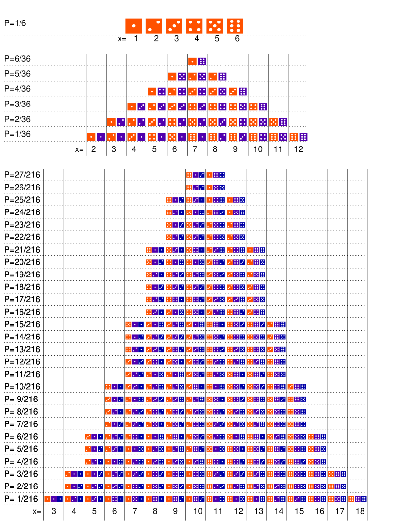
Figure 1: The probability distribution $P(x)$ of statistical outcomes $x$ are shown for tossing one (top panel), two (second panel), and three dice (bottom panel). The possible outcomes cover the ranges of $x=x_{1}=1,...,6$ for one dice, $x=(x_{1}+x2)=2,...,12$ for two dice, and $x=(x_{1}+x_{2}+x_{3})=3,...,18$ for three dice. The probability distributions are also known as binomial distributions and converge to a Gaussian distribution for an infinite number of dice.

The simplest statistical distribution is obtained from rolling dice, by enumerating all possible outcomes. The PDF of outcomes of rolling one dice, two dice, and three dice is shown in Fig. 1, the classical binomial distribution that approaches a Gaussian normal distribution (Fig. 1) for a large number of dice, with possible outcomes of $n\leq x\leq 6n$ for 6-sided dice, while the PDF $N(x)dx$ is a Gaussian function centered at $x=n(6+1)/2$.

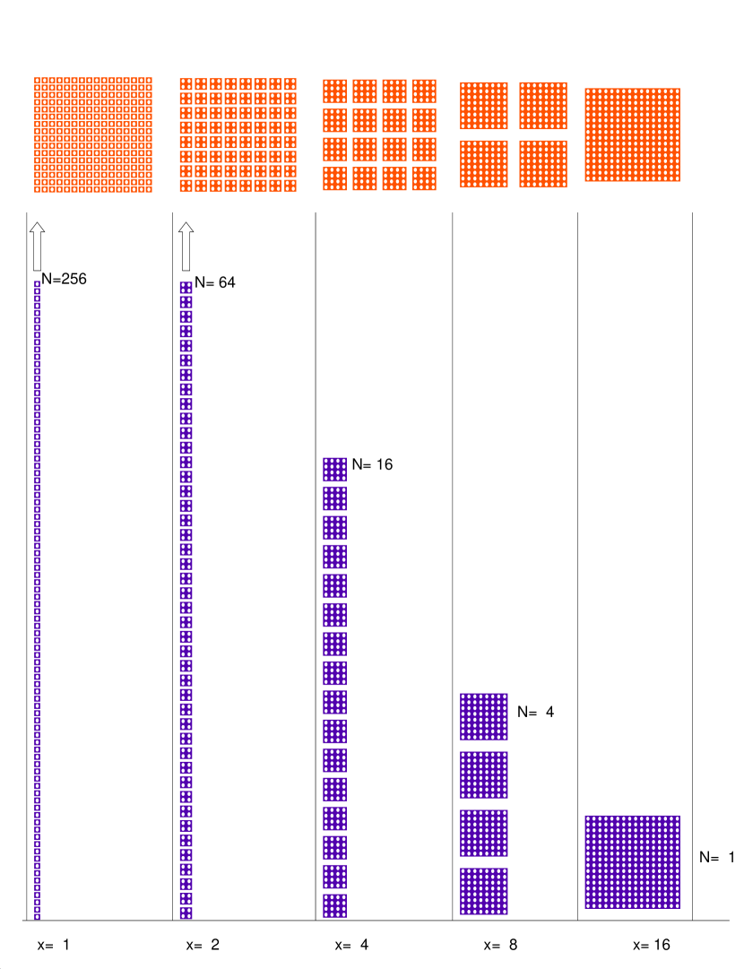
Figure 2: The probability distributions $N(x)$ of statistical outcomes $x$ are shown for braking domino pieces with square-like shape into smaller squares with side lengths that correspond to powers of two (i.e., x=1,2,4,8,16). A histogram with such logarithmic bins shows the number of outcomes, $N(x=1)=256=2^{5}$, $N(x=2)=64=2^{4}$, …., $N(x=16)=1$, which form a powerlaw distribution $N(x)\propto x^{-2}$ with a slope of $\alpha=\log{(N)}/\log{(x)}=-2$.

Going to the statistical probability distributions of avalanches with size $L$, we use the same method by enumerating all possible states with size $L$ that can occur in a SOC system with finite size $L_{2}$. The case with an Euclidean space dimension of $d=2$ is illustrated in Fig. 2, where we use logarithmic bins with size $x=1,2,4,8,16$. In a system with finite size $L_{2}=16$, one avalanche of this maximum size $L_{2}$ is possible in a given time interval, and thus $N(x=16)=1$. For a bin with half the size, $L=L_{2}/2=8$ we have four possible areas with a length scale of $x=L_{2}/2$, and thus $N(x=8)=4$. Proceeding to quarter bins, $L=L_{2}/4$, we have 16 possible areas with size $L=L_{2}/4$, and thus $N(x=4)=16=2^{4}$, and so forth. Obviously, the probability distribution scales as $N(x)dx=(L_{2}/L)^{2}$ for Euclidean dimension $d=2$. We can easily imagine the probabilities for the other Euclidean dimensions $d=1$, which is $N(x)dx=(L_{2}/L)$, and for $d=3$, which is $N(x)dx=(L_{2}/L)^{3}$. Therefore we obtain a generalized probability distribution of length scales $L$ according to

$$N(L)dL\propto L^{-d}\ dL\ ,$$ (1)

which we call the scale-free probability conjecture (Aschwanden 2012a), being related to packing rules (e.g., sphere packing, or dense packing) in geometric aggregation problems. A similar approach of using geometric scaling laws was also pioneered for earthquakes (Main and Burton 1984). The term scale-free is generally used to express that no special scale is present in a statistical distribution, unlike the first moment or center value of a Gaussian (normal) distribution, or the e-folding value in an exponential distribution. Our scale-free probability does not require that all possible avalanches in a SOC system have to occur simultaneously, or in any particular sequential order. They just represent the expected distribution of a statistically representative sample, similar to the rolling of dice. For instance, using $n=10^{26}$ dice to mimic the number of atoms per $cm^{3}$, there is no way to execute all possible rolls, but we expect for any statistically representative subset of possible outcomes a Gaussian distribution. Similarly, we expect a length distribution $N(L)$ according to Eq. (1) for any statistically representative subset of avalanches occurring in a SOC system. We expect that Eq. (1) has universal validity in SOC systems, because it is only based on a statistical argument of random processes on all scales, without any other constraints given by specific physical parameters or the dynamic behavior of a SOC system. This scale-free probability conjecture (Eq. 1) may also occur in other nonlinear systems, such as in turbulence. We may be able to discriminate between the two systems by the sparseness of avalanches (in slowly-driven SOC systems) and the space-filling of structures (in turbulent media).

2.2 Geometric Scaling Laws

In the following we are going to derive size distributions of SOC avalanches by using geometric scaling laws, which is a standard approach that has been applied in a number of previous work (e.g., Bak et al. 1988; Robinson 1994; Munoz et al. 1999; Biham et al. 2001).

Besides the length scale $L$, other geometric parameters are the Euclidean area $A$ or the Euclidean volume $V$. The simplest definition of an area $A$ as a function of a length scale $L$ is the square-dependence,

$$A\propto L^{2}\ ,$$ (2)

which applies also to circular areas, $A\propto\pi r^{2}$, or more complicated solid areas, differing only by a constant factor for self-similar geometric shapes. A direct consequence of this simple geometric scaling law is that the statistical probability distribution of avalanche areas is directly coupled to the scale-free probability distribution of length scales (Eq. 1), and can be computed by substitution of $L(A)\propto A^{1/2}$ (Eq. 2), into the distribution of Eq. (1), $N(L)=N(L[A])=L[A]^{-d}=(A^{1/2})^{-d}=A^{-d/2}$, and with the derivative $dL/dA\propto A^{-1/2}$,

$$N(A)dA\propto N(L[A])\left|{dL\over dA}\right|dA\propto A^{-(1+d)/2}\ dA\ .$$ (3)

Thus we expect an area distribution $N(A)$ depending on the dimensionality $d=2,3$ of the SOC system,

$$N(A)dA\propto A^{-\alpha_{A}}dA\qquad{\rm where}\ \left\{\begin{array}[]{ll}\alpha_{A}=1.5&{\rm for}\ d=2\\ \alpha_{A}=2.0&{\rm for}\ d=3\\ \end{array}\right.\ ,$$ (4)

which should also have universal validity for SOC systems. In spatially resolved astrophysical observations, such as of the Sun or magnetosphere, a length scale $L$ or area $A$ are the only directly measurable geometric parameters, while a volume $V$ is generally derived from the observed area of a SOC event.

Similarly to the area, we can derive the geometric scaling for volumes $V$, which simply scales with the cubic power in 3D space,

$$V\propto L^{3}\ ,$$ (5)

which represents a cube, but differs only by a constant factor for a sphere, i.e., $V=(4\pi/3)r^{3}$. Consequently, we can also derive the probability distribution $N(V)dV$ of volumes $V$ directly from the scale-free probability conjecture (Eq. 1), where the definition of Eq. (5) demands $d=3$. Substituting $L\propto V^{1/3}$ into $N(L[V])\propto L[V]^{d}\propto V^{-d/3}$ and the derivative $dL/dV=V^{-2/3}$ we obtain for $d=3$,

$$N(V)dV\propto N(L[V])\left|{dL\over dV}\right|dV\propto V^{-\alpha_{V}}\ dV\propto V^{-5/3}\ dV\ .$$ (6)

Thus, a powerlaw slope of $\alpha_{V}=5/3$ is predicted in 3D Euclidean space, which applies also to the Euclidean volume of a time-integrated SOC avalanche in lattice simulations. However, since avalanches have a fractal geometry, it is the time-integrated fractal volume that is equivalent to the number of active pixels in a lattice simulation, rather than the Euclidean volume.

Since all the assumptions made so far are universal, such as the scale-free probability conjecture (Eq. 1) and the geometric scaling laws $A\propto L^{2}$ and $V\propto L^{3}$, the resulting predicted occurrence frequency distributions of $N(A)$ (Eq. 3) and $N(V)$ (Eq. 6) are universal too, and powerlaw functions are predicted from this derivation from first principles, which is consistent with the property of universality in theoretical SOC definitions.

2.3 The Fractal Geometry

“Fractals in nature originate from self-organized critical dynamical processes” (Bak and Chen 1989). Fractal geometries have been pioneered in the context of self-similar structures before the advent of SOC models (Mandelbrot 1977, 1983, 1985), and have been applied to spatio-temporal SOC structures extensively (e.g., Bak et al. 1987, 1988; Bak and Chen 1989; Ito and Matsuzaki 1990; Feder and Feder 1991; Rinaldo et al. 1993; Erzan et al. 1995; Barabasi et al. 1995). Since the fractal geometry is a postulate of SOC processes invoked by the first pioneers of SOC, it is appropriate to approximate spatial structures of SOC avalanches by a fractal dimension. The simplest fractal is the Hausdorff dimension $D_{d}$, which is a monofractal and depends on the Euclidean space dimension $d=1,2,3$. The Hausdorff dimension $D_{3}$ for the 3D Euclidean space ($d=3$) is

$$D_{3}={\log{V_{f}(t)}\over\log{(L)}}\ ,$$ (7)

and analogously for the 2D Euclidean space ($d=2$),

$$D_{2}={\log{A_{f}(t)}\over\log{(L)}}\ ,$$ (8)

with $A_{f}(t)$ and $V_{f}(t)$ being the fractal area and volume of a SOC avalanche during an instant of time $t$. These fractal dimensions can be determined by a box-counting method, where the area fractal $D_{2}$ can readily be obtained from images from the real world, while the volume fractal $D_{3}$ is generally not available unless one obtains 3D data (or by numerical simulations).

A good approximation for the expected fractal dimension $D_{d}$ is the mean value of the smallest possible fractal dimension $D_{d,min}\approx 1$ and the largest possible fractal dimension $D_{d,max}=d$. The minimum possible fractal dimension is near the value of 1 because the next-neighbour interactions in SOC avalanches require some continuity between active nodes in a lattice simulation of a cellular automaton, while smaller fractal dimensions $D_{d}<1$ are too sparse to allow an avalanche to propagate via next-neighbor interactions. Thus, the mean value of a fractal dimension is expected to be (Aschwanden 2012a),

$$D_{d}\approx{D_{d,min}+D_{d,max}\over 2}={(1+d)\over 2}\ .$$ (9)

Thus, we expect fractal dimensions of $D_{3}\approx(1+3)/2=2.0$ for the 3D space, and $D_{2}\approx(1+2)/2=1.5$ for the 2D space. This conjecture of the mean value of the fractal dimension $D_{d}$ has been numerically tested with cellular automaton simulations for Eucledian dimensions $d=1,2,3$ and the following mean values were found: $D_{1}=1.00\pm 0.00$ (Aschwanden 2012a); then $D_{2}=1.58\pm 0.02$ (Charbonneau et al. 2001), $D_{2}=1.58\pm 0.03$ (McIntosh et al. 2002), $D_{2}=1.60\pm 0.17,1.62\pm 0.18$ (Aschwanden 2012a) for the 2D case, for which $D_{2}=1.5$ is predicted, and $D_{3}=1.78\pm 0.01$ (Charbonneau et al. 2001, McIntosh et al. 2002), $D_{3}=1.94\pm 0.27,1.97\pm 0.29$ (Aschwanden 2012a) for the 3D case, for which $D_{3}=2.0$ is predicted. Thus, the mean value defined in Eq. (9) is a reasonably accurate prediction based on the standard (BTW) cellular automaton model.

This relationship (Eq. 9) allows also a scaling between the fractal dimensions of the 2D and 3D Euclidean space,

$${D_{3}\over D_{2}}\approx{(1+3)\over(1+2)}={4\over 3}\ .$$ (10)

An extensive discussion of measuring the fractal geometry in SOC systems is given in Aschwanden (2011a, chapter 8) and McAteer (2013). Fractals are measurable from the spatial structure of an avalanche at a given instant of time. Therefore, they enter the statistics of time-evolving SOC parameters, such as the observed flux per time unit, which is proportional to the number of instantaneously active nodes in a lattice-based SOC avalanche simulation.

2.4 The Spatio-Temporal Evolution and Transport Process

The next important step is to include time scales, which together with the geometric scaling laws define the spatio-temporal evolution of SOC events. We model a SOC event simply as an instability that is triggered when a local threshold is exceeded. The universal behavior of any instability is an initial nonlinear growth phase and a subsequent saturation phase. We model the saturation phase with a diffusive function, as shown in Fig. 3 (upper panel),

$$r(t)=\kappa(t-t_{0})^{\beta/2}\ .$$ (11)

where $t_{0}$ is the onset time of the instability, $\kappa$ is the diffusion coefficient, and $\beta$ is the spreading exponent. A value of $\beta\lower 1.72218pt\hbox{$\;\buildrel>\over{\scriptstyle\sim}\;$}0$ corresponds to logistic growth with an upper limit of the spatial volume (Aschwanden 2011a, 2012b), $\beta\approx 0.5$ corresponds to subdiffusion, $\beta=1$ to classical diffusion, $\beta\approx 1.5$ to hyper diffusion or Lévy flight, and $\beta=2$ to linear expansion.

The corresponding velocity $v(t)$ of an expanding SOC avalance is shown in Fig. 3 (second panel), which monotonically decreases with time and is obtained from the time derivative of $r(t)$ (Eq. (11),

$$v(t)={dr(t)\over dt}={\kappa\beta\over 2}\ (t-t_{0})^{\beta/2-1}\ .$$ (12)

What spatio-temporal scaling law do we expect from this macroscopic description of a SOC avalanche. A spatial scale $L$ could be defined from the maximum size of the avalanche at the end time $T=(t-t_{0})$, and thus we expect from Eq. (11) the statistical spatio-temporal scaling law

$$L\propto\kappa\ T^{\beta/2}\ .$$ (13)

Substituting this scaling law $L(T)$ into the PFD of length scales (Eq. 1), we expect a powerlaw distribution of time scales,

$$N(T)dT=N(L[T]){dL\over dT}dT=T^{-[1+(d-1)\beta/2]}=T^{-\alpha_{T}}\ .$$ (14)

with the powerlaw slope of $\alpha_{T}=1+(d-1)\beta/2$, which has a value of $\alpha_{T}=1+\beta=2.0$ for 3D-Euclidean space $(d=3)$ and classical diffusion ($\beta=1$). This powerlaw slope for avalanche time scales is a prediction of universal validity, since it is only based on the scale-free probability conjecture (Eq. 1), $N(L)\propto L^{-d}$, and the diffusive nature (or random-walk statistics) of the saturation phase.

The spatio-temporal scaling law (Eq. 13), based on random-walk or a diffusion process, is used here as a simple approximation in an empirical way. Diffusive transport has been applied to SOC theory and SOC phenomena in a number of previous studies, e.g., by using the spreading exponents to determine the critical points of systems with multiple absorbing states (Grassberger and Delatorre 1979), as a discretized diffusion process using the Langevin equation (Wiesenfeld 1989; Zhang 1989; Foster et al. 1977; Medina et al. 1989), in terms of classical (Lawrence 1991) and anomalous diffusion of magnetic flux events (Lawrence and Schrijver 1993), in deriving spatio-temporal scaling laws with mean-field theory and branching theory (Vespignani and Zapperi 1998), as a continuum limit of a fourth-order hyper-diffusive system (Liu et al. 2001; Charbonneau et al. 2001), or in terms of a diffusion entropy description (Grigolini et al. 2002).

2.5 Energy and Flux Relationships

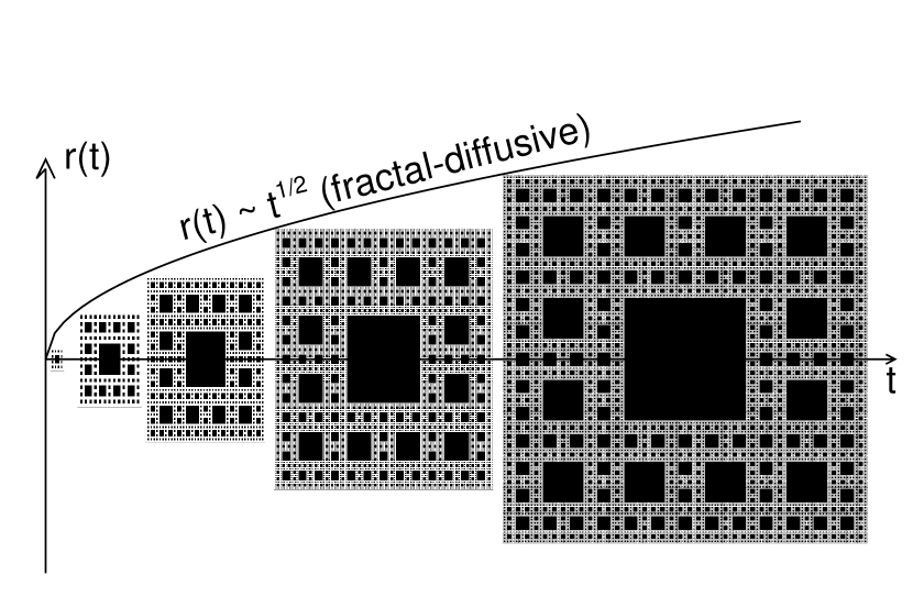
Figure 4: A cartoon that illustrates the concept of fractal-diffusive avalanche evolution. The Euclidean radius $r(t)$ evolves like a diffusive random walk, such as $r(t)\propto t^{1/2}$ for classical diffusion, while the avalanche area is fractal (black substructures). The instantaneous fractal area $A_{f}(t)\propto r(t)^{D_{t}}$ consists of the number active nodes and is proportional to the energy dissipation rate $dE(t)/dt$ or flux $F(t)$ at a given time $t$.

In numerical SOC simulations, such as in lattice-based cellular automaton models of the BTW type (Bak et al. 1987), energy is dissipated in every node that exceeds a threshold temporarily, and thus the energy that is dissipated during a SOC avalanche is proportional to the total number of all active nodes, summed over space at each instant of time. If we count these active nodes at a given time interval, we have a quantity that is proportional to the instantaneous energy dissipation rate, which has the unit of energy per time. In the real world we observe a signal from a SOC avalanche in form of an intensity flux $f(t)$ (e.g., seismic waves from earthquakes, hard X-ray flux from solar flares, or the amount of lost dollars per day in the stockmarket). Let us assume that this intensity flux is proportional to the volume of active nodes, which corresponds to the instantaneous fractal volume $V_{f}(t)$ of a SOC avalanche in our spatio-temporal SOC model (Fig. 4), also called fractal-diffusive (FD-SOC) model (Aschwanden 2012a),

$$f(t)\propto V_{f}(t)\propto r(t)^{D_{d}}\ ,$$ (15)

which is shown in Fig. 3 (third panel) for $\beta=$0.1, 0.5, and 1. The flux time profile $f(t)$ is expected to fluctuate substantially in real data or in lattice simulations, because the fractal dimension can vary in the range of $D_{d,min}\approx 1$ and $D_{max}=d$, while we use only the mean value $D_{d}=(D_{min}+D_{max})/2$ (Eq. 9) in our macroscopic model. Occasionally, the instantaneous fractal dimension may reach its maximum value, i.e., $D_{d}(t)\lower 1.72218pt\hbox{$\;\buildrel<\over{\scriptstyle\sim}\;$}d$, which defines an expected upper limit $f_{max}(t)$ of

$$f_{max}(t)\propto V(t)\propto r(t)^{d}\ .$$ (16)

Integrating the time-dependent flux $f(t)$ over the time interval $[0,t]$ yields the total dissipated energy $e(t)$ up to time $t$ (using Eq. 11),

$$e(t)\propto\int_{0}^{t}V_{f}(t)dt=\int_{0}^{t}r^{D_{d}}(t)dt=\int_{0}^{t}\kappa^{D}_{d}(t-t_{0})^{D_{d}\beta/2}dt={\kappa^{D_{d}}\over D_{d}\beta/2+1}(t-t_{0})^{D_{d}\beta/2+1}\ ,$$ (17)

which is a monotonically increasing quantity with time (Fig. 3, bottom panel).

From this time-dependent evolution of a SOC avalanche we can characterize at the end time $t$ a time duration $T=(t-t_{0})$, a spatial scale $L=r(t=t_{0}+T)$, an expected flux or energy dissipation rate $F=f(t=t_{0}+T)$, an expected peak flux or peak energy dissipation rate $P=f_{max}(t=t_{0}+T)$, and a dissipated energy $E=e(t=t_{0}+T)$, which is proportional to the avalanche size $S$ in BTW models. Thus, we have the following scaling relations between the different SOC parameters and the length scale $L$ (using Eqs. 15-17),

$$F\propto L^{D_{d}}\propto T^{D_{d}\beta/2},$$ (18)

$$P\propto L^{d}\propto T^{d\beta/2}\ ,$$ (19)

$$E\propto S\propto L^{D_{d}+2/\beta}\propto T^{D_{d}\beta/2+1}\ .$$ (20)

An alternative notation for the diffusive spreading exponent $\beta$ used in literature is $D_{T}=2/\beta$, so that the spatio-temporal scaling law (Eq. 13) reads as $T\propto L^{D_{T}}$ and the energy scaling law (Eq. 20) as $E=S\propto V_{f}T\propto L^{D_{d}+D_{T}}$, which can be expressed as $S\propto L^{D_{S}}$ with the exponent $D_{S}=D_{3}+D_{T}$. Slight variations of this scaling law have been inferred from observations in different wavelengths, such as $D_{S}=D_{A}/2+D_{T}$ for magnetic events (Eq. 18 in Uritsky et al. 2013), which seems to be equally consistent with observations as our generalized (wavelength-independent) FD-SOC model (see EIT and MDI events from Udritsky et al. 2013 in Table 1).

Finally we want to quantify the occurrence frequency distributions of the the (smoothed) energy dissipation rate $N(F)$, the peak flux $N(P)$, and the dissipated energy $N(E)$, which all can readily be obtained by substituting the scaling laws (Eqs. 18-20) into the fundamental length scale distribution (Eq. 1), yielding

$$N(F)dF=N(L[F])\left|{dL\over dF}\right|dF\propto F^{-[1+(d-1)/D_{d}]}\ dF\ ,$$ (21)

$$N(P)dP=N(/[P])\left|{dL\over dP}\right|dP\propto P^{-[2-1/d]}\ dP\ ,$$ (22)

$$N(E)dE=N(L[E])\left|{dL\over dE}\right|dE\propto E^{-[1+(d-1)/(D_{d}+2/\beta)]}\ dE\ .$$ (23)

Thus this derivation from first principles predicts powerlaw functions for all parameters $L$, $T$, $F$, $P$, $E$, and $S$, which are the hallmarks of SOC systems. In summary, if we denote the occurrence frequency distributions $N(x)$ of a parameter $x$ with a powerlaw distribution with power law index $\alpha_{x}$,

$$N(x)dx\propto x^{-\alpha_{x}}\ dx\ ,$$ (24)

we have the following powerlaw coefficients $\alpha_{x}$ for the parameters $x=L,T,F,P,E$, and $S$,

$$\begin{array}[]{rl}\alpha_{L}&=d\\ \alpha_{T}&=1+(d-1)\beta/2\\ \alpha_{F}&=1+(d-1)/D_{d}\\ \alpha_{P}&=1+(d-1)/d\\ \alpha_{E}=\alpha_{S}&=1+(d-1)/(D_{d}+2/\beta)\\ \end{array}\ .$$ (25)

If we restrict to the case to 3D Euclidean space (d=3), as it is almost always the case for real world data, the predicted powerlaw indexes are,

$$\begin{array}[]{rl}\alpha_{L}&=3\\ \alpha_{T}&=1+\beta\\ \alpha_{F}&=1+2/D_{3}\\ \alpha_{P}&=1+2/3\\ \alpha_{E}=\alpha_{S}&=1+1/(D_{3}/2+1/\beta)\\ \end{array}\ .$$ (26)

Restricting to classical diffusion $(\beta=1)$ and an estimated mean fractal dimension of $D_{3}\approx(1+3)/2=2$ we have the following absolute predictions

$$\begin{array}[]{rl}\alpha_{L}&=3\\ \alpha_{T}&=2\\ \alpha_{F}&=2\\ \alpha_{P}&=5/3\\ \alpha_{E}=\alpha_{S}&=3/2\\ \end{array}\ .$$ (27)

2.6 Waiting Time Probabilities in the Fractal-Diffusive SOC Model

The FD-SOC model predicts a powerlaw distribution $N(T)\propto T^{-\alpha_{T}}$ of event durations $T$ with a slope of $\alpha_{T}=[1+(d-1)\beta/2]$ (Eq. 25) that derives directly from the scale-free probability conjecture $N(L)\propto L^{-d}$ (Eq. 1) and the random walk (diffusive) transport ($L\propto T^{\beta/2}$; Eq. 13). For classical diffusion ($\beta=1$) and space dimension $d=3$ the predicted powerlaw is $\alpha_{T}=2$. From this time scale distribution we can also predict the waiting time distribution with a simple probability argument. If we define a waiting time $\Delta t$ as the time interval between the start time of two subsequent events, so that no two events overlap with each other temporally, the waiting time cannot be shorter than the time duration of the intervening event, i.e., $\Delta t_{i}\geq(t_{i+1}-t_{i})$. Let us consider the case of non-intermittent, contiguous flaring, but with no time overlap between subsequent events. In this case the waiting times are identical with the event durations, and therefore their waiting time distributions are equal also, reflecting the same statistical probabilities,

$$N(\Delta t)d\Delta t\propto N(T)dT\propto\Delta t^{-\alpha_{\Delta t}}d\Delta t\ ,$$ (28)

with the powerlaw slope,

$$\alpha_{\Delta t}=\alpha_{T}=1+(d-1)\beta/2\ .$$ (29)

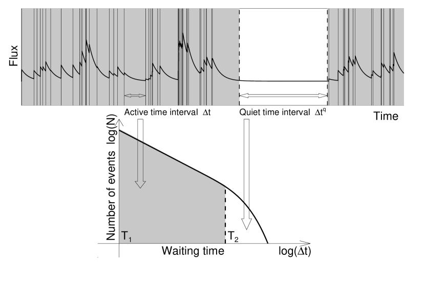
Figure 5: The concept of a dual waiting time distribution is illustrated, consisting of active time intervals $\Delta t\lower 1.72218pt\hbox{$\;\buildrel<\over{\scriptstyle\sim}\;$}T_{2}$) that contribute to a powerlaw distribution (which is equal to that of time durations, $N(T)$), and random-like quiet time intervals ($\Delta t^{q}$) that contribute to an exponential cutoff.

This statistical argument is true regardless what the order of subsequent event durations is, so it fulfills the Abelian property. Now we relax the contiguity condition and subdivide the time series into blocks with contiguous flaring (with intervals $\Delta t\approx T$), interrupted by arbitrarily long quiet periods $\Delta t=\Delta t^{q}$ when no events occur (Fig. 5). The distribution of quiet periods $\Delta t^{q}$ may be drawn from a random process, which has an exponential distribution

$$N(\Delta t^{q})d\Delta t^{q}\propto\exp{(-\Delta t^{q}/\Delta t^{q}_{0})}\ d\Delta t^{q}\ .$$ (30)

If we define a maximum event duration $T_{2}$ and assume that this is also approximately a lower limit for the quiet time intervals, i.e., $\Delta t^{q}_{min}\approx T_{2}$, then we expect a powerlaw distribution with a slope of $\alpha_{\Delta t}=\alpha_{T}$ for the range of waiting times that are shorter than the maximum flare duration $\Delta t\lower 1.72218pt\hbox{$\;\buildrel<\over{\scriptstyle\sim}\;$}T_{2}$, with an exponential cutoff at $\Delta t\lower 1.72218pt\hbox{$\;\buildrel>\over{\scriptstyle\sim}\;$}T_{2}$. The contributions of waiting times from the subset of contiguous time blocks will still be identical, while those time intervals from the intervening quiet periods add some longer random waiting times. The predicted powerlaw slope of short waiting times ($T_{1}\lower 1.72218pt\hbox{$\;\buildrel<\over{\scriptstyle\sim}\;$}\Delta t\lower 1.72218pt\hbox{$\;\buildrel<\over{\scriptstyle\sim}\;$}T_{2}$) is then $\alpha_{\Delta t}=2.0$ for classical diffusion $\beta=1$ and space dimension $d=3$. Interestingly, this predicted slope is identical to that of nonstationary Poisson processes in the limit of intermittency (Aschwanden and McTiernan 2010). At the same time, this waiting time model predicts also clustering of events during active periods, and thus event statistics with memory and persistence, as it was demonstrated recently for CME events using Weibull distributions (Telloni et al. 2014).

2.7 Pulse Pile-Up Correction for Waiting Times

We can define a mean waiting time $\langle\Delta t\rangle$ from the total duration of the observing period $T_{obs}$ and the number of observed events $n_{obs}$,

$$\langle\Delta t\rangle={T_{obs}\over n_{obs}}\ .$$ (31)

From the distribution of event durations $T$, we have an inertial range of time scales $[T_{1},T_{2}]$, over which we observe a powerlaw distribution, $N(T)\propto T^{-\alpha_{T}}$, with the corresponding number of events $[N_{1},N_{2}]$, so that we can define a nominal powerlaw slope of $\alpha_{T}=\log(N_{2}/N_{1})/\log(T_{2}/T_{1})$. If the mean waiting time of an observed time series becomes shorter than the upper limit of time scales $T_{2}$ during very busy periods, we start to see time-overlapping events, a situation we call “event pile-up” or “pulse pile-up”. In such a case we expect that the waiting time distribution starts to be modified, because the time durations of the long events are underestimated (by some automated detection algorithm), so that the nominal powerlaw slope that is expected with no pulse pile-up, $\alpha_{\Delta t}=\log(N_{2}/N_{1})/\log(T_{2}/T_{1})$, has to be modified by replacing the lower time scale $T_{1}$ with the mean waiting time $\langle\Delta t\rangle$,

$$\alpha_{\Delta t}^{pileup}\ =\ \alpha_{\Delta t}\times\left\{\begin{array}[]{ll}1&{\rm for}\ \langle\Delta t\rangle\ >\ T_{2}\\ \log(T_{2})/\log{\langle\Delta t\rangle}&{\rm for}\ \langle\Delta t\rangle\ \leq\ T_{2}\\ \end{array}\right.$$ (32)

As a consequence, the measurements of event durations must suffer from the same pile-up effect, and a similar correction is expected for the time scale distribution $N(T)$,

$$\alpha_{T}^{pileup}\ =\ \alpha_{T}\times\left\{\begin{array}[]{ll}1&{\rm for}\ \langle\Delta t\rangle\ >\ T_{2}\\ \log(T_{2})/\log{\langle\Delta t\rangle}&{\rm for}\ \langle\Delta t\rangle\ \leq\ T_{2}\\ \end{array}\right.$$ (33)

Thus the predicted waiting time distribution has a slope of $\alpha_{T}=2$ in the slowly-driven limit, but can be steeper in the strongly-driven limit. For instance, the waiting time distributions of solar flares correspond to the slowly-driven limit during the minima of the solar 11-year cycle, while the powerlaw slopes indeed steepen during the maxima of the solar cycle (Aschwanden and Freeland 2012), when the flare density becomes so high that the slowly-driven limit, and thus the separation of time scales, is violated.

2.8 Physical Scaling Laws

Our fractal-diffusive SOC model developed so far has universal validity because it is entirely derived from statistical probabilities and fractal-diffusive transport. The predicted scaling laws and occurrence frequency distributions derived above do not depend on any specific physical parameter of a SOC phenomenon. Using real-world observations, however, some physical scaling laws are involved between the observables and the spatio-temporal parameters used so far. For instance, the strength of an earthquake is measured in magnitudes of the Gutenberg-Richter scale (Richter 1958), which may be related to the observed earthquake rupture area by some mechanical scaling law that determines the statistics (Main and Burton 1984). For solar flares, the observed fluxes in soft or hard X-rays are related to the physical parameters of electron temperatures, densities, and pressures of heated plasma, as it can be derived for the equilibrium point between heating and cooling (e.g., Rosner et al. 1978). Other scaling laws used in solar physics include, for instance, relationships between magnetic energies and the reduced MHD equations (Longcope and Sudan 1992), or the magnetic reconnection geometry (Craig 2001), or between the heating rate and the magnetic field strength (Schrijver et al. 2004). Such physical scaling laws allow us to derive the powerlaw slope of the frequency distribution of both the observables and the physical parameters, which is examined elsewhere (e.g., Aschwanden et al. 2013).

The predicted frequency distributions for energies and fluxes derived in Section 2.5, are strictly only valid for systems where the assumption of proportionality between the flux and the instantaneous fractal volume is fulfilled, i.e., $F(t)\propto V_{f}(t)\propto r(t)^{D_{d}}$ (Eq. 15), because the scaling of observables depends then on geometric parameters only, which can be derived entirely from statistical probabilities, in terms of the scale-free probability conjecture (Eq. 1).

Without specializing on a particular physical mechanism of a given SOC system, we can give some general rules how to derive the powerlaw function of physical parameters. The simplest situation is a 2-parameter correlation or scaling law, where a physical parameter $x$ is related to the geometric length scale by a powerlaw function with index $\gamma$,

$$L\propto x^{\gamma}\ .$$ (34)

Inserting this scaling law into the fundamental length scale distribution $N(L)\propto L^{-d}$ (Eq. 1) and using the derivative $dL/dx=x^{\gamma-1}$ yields then directly the occurrence frequency distribution $N(x)$,

$$N(x)dx=N(L[x]){dL\over dx}dx=x^{-[1+(d-1)\gamma]}dx\ .$$ (35)

Also common is a 3-parameter correlation or scaling law, such as in terms of two physical parameters $x$ and $y$ and the length scale $L$, i.e.,

$$L\propto x^{\gamma}y^{\delta}\ ,$$ (36)

in terms of powerlaw functions with exponents $\gamma$ and $\delta$. The probability distribution for one of the physical parameters, say $y$, can then be written as,

$$N(y)dy=\int N(L,x[L,y])dL\ dy=\int N(L)N(x[L,y])dL\ dy\propto y^{a_{x}\delta/\gamma}\ dy\ ,$$ (37)

after the integration over the variable $L$ is carried out. Thus the resulting distribution $N(y)dy\propto y^{-\alpha_{y}}dy$ has a powerlaw slope of $\alpha_{y}=\alpha_{x}\delta/\gamma$. The powerlaw solution is strictly valid only for complete sampling of the parameters, which in reality is often not possible due to limited statistics, instrumental sensitivity limits, and data noise. This leads to truncation effects and finite-size effects, which can be simulated with Monte-Carlo simulations or analytically calculated (see Appendix in Aschwanden et al. 2013 for examples).

2.9 Instrument-Dependent Size Distributions

Besides physical scaling laws that are specific to a particular physical mechanism of a SOC system, there are also instrument-dependent scaling laws that are not universal and depend on the specific instrument used in an observation of SOC phenomena. If there is a nonlinear scaling between the observable and the geometric volume of a SOC avalanche, we cannot expect to measure the same powerlaw slope of an observable with different instruments. In order to make observed frequency distributions obtained with different instruments compatible, it is often advisable to reduce the observable parameters to physical parameters using a well-established instrument calibration. For astrophysical observations in soft X-rays and EUV, for instance, an instrument-independent physical quantity is the differential emission measure distribution, which can be inverted from observed fluxes in different wavelengths (e.g., Aschwanden et al. 2013).

3 RELATIONSHIP TO THEORETICAL MICROSCOPIC SOC MODELS

After we have described a general macroscopic model of a SOC system that predicts the occurrence frequency distributions of spatial, temporal, and volume-related observables, such as the flux and energy, we turn now to theoretical and numerical SOC models and discuss whether our macroscopic model meets the basic definitions of a SOC system. A comprehensive review of theoretical and numerical SOC models is given in the textbook by Pruessner (2012). While a strict definition of SOC systems is still not well-established, we will use here the working definition given in the Introduction: SOC is a critical state of a nonlinear energy dissipation system that is slowly and continuously driven towards a critical value of a system-wide instability threshold, producing scale-free, fractal-diffusive, and intermittent avalanches with powerlaw-like size distributions. The property of self-tuning to criticality is warranted by system-inherent physical conditions that define a system-wide instability threshold. This system-inherent physical condition is often given by the equilibrium solution between two competing forces. For instance, the angle of repose in a sandpile is self-tuning to a system-wide critical value, corresponding to an equilibrium point between the gravity force and the static friction force. In the Ising model (Ising 1925), a phase transition occurs at a critical point between an ordered and a disordered magnetic spin state, but the tuning to the critical point is not self-organized. In the following we discuss how the macroscopic SOC model (Section 2) relates to the microscopic (mathematical and numerical) SOC models, regarding powerlw-scaling (Section 3.1), spatio-temporal correlations (Section 3.2), separation of time scales and intermittency (Section 3.3), and self-tuning and critical threshold (Section 3.4).

3.1 Powerlaw Scaling

The original Bak-Tang-Wiesenfeld (BTW) model revealed the generic scale invariance of simulated or observed SOC parameters, which ideally exhibits powerlaw functions for the occurrence frequency distributions, possibly related to the 1/f-noise of power spectra (Bak et al. 1987). The property of a powerlaw shape became the hallmark of SOC phenomena, but it was recognized that this is a necessary but not a satisfactory condition, since other phenomena (such as turbulence or percolation) produce powerlaws also.

Our fractal-diffusive SOC model (FD-SOC) derives the probability distribution functions (PFD) based on a statistical probability argument, which leads to a powerlaw function of spatial and geometric scales. The additional assumption of fractal-diffusive transport leads to a powerlaw function of temporal scales. Further we define the size of an avalanche from the time-integrated fractal volume that participates in an avalanche, and consequently we obtain also powerlaw distributions for the size or total dissipated energy of avalanches. Since all these assumptions are of statistical nature and do not depend on any physical parameters of a SOC system, the predictions of the PDFs of spatial, temporal, and energy SOC parameters have universal applicability, irregardless of the physical process that is involved in the nonlinear energy dissipation process. The prediction of a pure powerlaw function for the size distributions at all scales is also called universality in theoretical SOC models (e.g. Sethna et al. 2001), and is fulfilled in the macroscopic description of our FD-SOC model by design (as a consequence of the scale-free probability conjecture; Eq. 1). However, we should be aware that this simple FD-SOC model provides only a first-order prediction, while additional effects (such as truncation, incomplete sampling, or finite-size effects) may modify the observed size distributions into broken powerlaws, double powerlaws, or other powerlaw-like distribution functions. However, similar effects occur also in cellular automaton simulations.

3.2 Spatio-Temporal Correlations

SOC systems are expected to exhibit spatio-temporal correlations (Jensen 1998) of a SOC state variable ${\bf B({\bf r},t)}$,

$$C({\bf r},t)=<B({\bf r}_{0},t_{0})B({\bf r}_{0}+{\bf r},t_{0}+t)>-<{\bf B}({\bf r}_{0},t_{0})>^{2}\ .$$ (38)

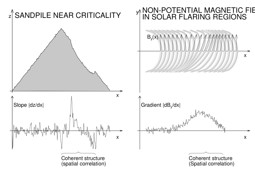
Figure 6: Left: A sandpile in a state in the vicinity of criticality is shown with a vertical cross-section $z(x)$, with the gradient of the slope (or repose angle) $|dz/dx|$ (bottom), exhibiting short-range fluctuations due to noise and long-range correlation lengths due to locally extended deviations from the mean critical slope. Right: The solar analogy of a flaring region is visualized in terms of a loop arcade over a neutral line in $x$-direction, consisting of loops with various shear angles that are proportional to the gradient of the field direction $B_{x}/B_{y}$, showing also some locally extended (non-potential) deviations from the potential field (bottom).

Such correlations are absent in systems with random noise. In our FD-SOC model, however, the random structure of the background in a state near criticality is episodically disturbed by an avalanche event, which carves out a “hole” with a size $L$ during a time scale $T$, which represents a major disturbance in form of a spatially and temporally coherent structure, which can be restored to the critical state only gradually, for slowly-driven SOC systems. Naturally, large avalanches leave their footprints behind and produce spatio-temporal correlations during the local restoration time. The correlation is best for large avalanches with similar shapes. The time profiles of avalanches in our FD-SOC system are self-similar to some extent, since they are characterized by a common fractal dimension $D_{d}$ (Eq. 15), diffusion constant $\kappa$, and diffusive spreading exponent $\beta$ (Eq. 11). We visualize the spatial correlations with a cartoon in Fig. 6, which shows coherent disturbances as deviations from the critical state in large avalanches occurring in sandpiles and in solar flares.

In our two-component model of waiting times (Section 2.6), an observed time series consist of quiet intervals $\Delta t^{q}>T_{2}$ with no avalanching (which have a random distribution), and active intervals with contiguous flaring (which have a powerlaw distribution like the event durations $N(\Delta t)=N(T)$). This dual behavior is also called intermittency, and has the consequence that the combined waiting time distribution has both a powerlaw range ($T_{1}\leq\Delta t\leq T_{2}$) and an exponential cutoff ($\Delta t\geq T_{2}$). Consequently, we expect spatio-temporal correlations (Eq. 38) during the intermittently active periods only, while they are expected to be absent during the quiet time intervals. Avalanching during active periods is also expected to exhibit persistence and memory, while no memory is expected during quiet time intervals. This property seems to be more consistent with observations (e.g., Telloni et al. 2014), but is different from the pure random (Poisson) statistics of the original BTW model, but reconciles related debates about the functional shape of the waiting time distributions (e.g., Boffetta et al. 1999; Lepreti et al. 2001).

3.3 Separation of Time Scales and Intermittency

Classical SOC systems operate in the limit of slow driving, which implies a separation between the duration of an avalanche and the waiting time interval between two subsequent avalanches. Numerically, the separation of time scales is simply realized by allowing only one single disturbance of a SOC system at a time, which triggers an avalanche (with duration $T$) or not, while the next disturbance is not initiated after a waiting time $\Delta t>T$, in the case of an avalanche.

In our FD-SOC model, the energy dissipation rate $(de/dt)$ is monotonically growing after a triggering disturbance, which exceeds the system-wide threshold value $(de/dt)_{crit}$ until the spatial diffusion stops after time $T$, due to a lack of unstable nodes among the next-neighbors of an instantaneous avalanche area or volume. Therefore, the energy dissipation rate during an avalanche exceeds the threshold value during the entire duration of an avalanche. Energy conservation between the slowly-driven energy input rate and the intermittent avalanching output rate can therefore only be obtained with sufficiently long waiting times $\Delta t$ during which the energy loss of an avalanche is restored. This requires a balance of the long-term averages of the energy input and output rates, i.e.,

$$\langle(de/dt)_{in}\rangle\langle\Delta t\rangle\approx\langle(de/dt)_{out}\rangle\langle T\rangle\ .$$ (39)

Since $\langle(de/dt)_{in}\rangle\leq(de/dt)_{crit}\ll\langle(de/dt)_{out}\rangle$, it follows that $\langle\Delta t\rangle\gg\langle T\rangle$, which warrants a separation of the time scales, i.e., the waiting time $\Delta t$ and the avalanche duration $T$.

The resulting time profile of the energy dissipation rate $(de/dt)$ of a SOC system is then necessarily highly intermittent due to the long waiting times inbetween subsequent avalanches. In addition, the time profile is strongly fluctuating during an avalanche, according to $f(t)\propto r(t)^{D_{d}}$ (Eq. 15), since the fractal dimension $D_{d}(t)$ can fluctuate in the entire range between the minimum and maximum value as a function of time, i.e., $1\lower 1.72218pt\hbox{$\;\buildrel<\over{\scriptstyle\sim}\;$}D_{d}(t)\leq d$. However, for the scaling laws in the FD-SOC model (Eqs. 18-20), we can replace the fluctuating value of $D_{d}(t)$ with a constant mean value $\langle D_{d}(t)\rangle=(1+d)/2$ and obtain the same size distributions.

3.4 Self-Organization and Criticality

How does our fractal-diffusive SOC model reinforce self-organized criticality? In classical SOC models, criticality is obtained by a slowly-driven input of energy which restores the energy losses of avalanches until the system-wide critical threshold is reached (more or less) and new avalanches can be triggered by a local excess of the critical threshold. In our FD-SOC model, the time evolution of an avalanche has a generic shape that is given by fractal-diffusive transport, while the energy balance between energy input (disturbances) and output (avalanches) is not explicitly reinforced, unlike cellular automaton models which iterate a mathematical redistribution rule to drive the dynamics of a SOC system and are designed to conserve energy. Instead, self-organization of the FD-SOC model is constrained by statistical probability only, which does not need to be self-tuning to produce a particular functional form of a size distribution, because there is only one statistical distribution with maximum likelyhood, which is a powerlaw distribution function of spatial scales (according to our scale-free probability conjecture). So, we can say that the FD-SOC model gravitates around the statistically most likely state, like entropy in self-contained statistical systems without external influence. This may be a more general definition of self-organized criticality then originally proposed by Per Bak and coworkers, but explains the concept of self-organization by the most general principle of maximum statistical likelyhood. This should not surprise us, since the entire evolution of our universe followed maximum statistical likelihood, from the initial big bang expansion all the way to the bio-chemical evolution of life, forming complexity out of simple structures based on processes that are driven by statistical likelyhood (e.g., Mendel’s law in genetics).

4 ASTROPHYSICAL APPLICATIONS

In this section we examine frequency distributions observed in various realms of astrophysics and discuss the application of the fractal-diffusive SOC model in a few selected datasets with large statistics. Some preliminary discussion of such astrophysical objects can also be found in Aschwanden (2011a; chapters 7 and 8) and in Aschwanden (2013; chapter 13). An overview of astrophysical phenomena with observed powerlaw indices of size distributions is given in Table 1.

4.1 Lunar Craters

If we mount a large container with a gel-like surface below a circular plate that holds Per Bak’s sandpile, we would record impact craters from each sandpile avalanche in the viscous gel and could infer the avalanche sizes from the diameters of the impact craters (see experimental setup of sandpile experiment conducted by Held et al. 1990). Similarly, the Moon was targeted by many impacting meteors and meteorites, especially during an intense bombardment in the final sweep-up of debris at the end of the formation of the solar system between 4.6 and 4.0 billion years ago (e.g., Neukum et al. 2001). The sizes of lunar craters were measured with the first lunar orbiters (Ranger 7, 8, 9) in the early 1960’s, and a cumulative powerlaw distribution with sizes in the range of $L\approx 10^{0}-10^{4.5}$ cm was found, with a powerlaw slope of $\alpha^{cum}_{L}\approx 2.0$ for the cumulative distribution (Cross 1966), which corresponds to a value of $\alpha_{L}=\alpha^{cum}_{L}+1=3.0$ for the differential size distribution. This quite accurate result (for a size distribution covering a range of over 4 orders of magnitude) corresponds exactly to our prediction of the scale-free probability conjecture, $N(L)\propto L^{-3}$ (Eq. 1). A similar value of $\alpha_{L}=2.75$ was found for the size distribution of meteorites and space debris from man-made rockets and satellites (Fig. 3.11 in Sornette 2004). The formation of the sizes of meteors and meteorites may have been controlled by a nonlinear process that includes a combination of self-gravity, gravitational disturbances, collisions, depletions, fragmentation, and captures of incoming new bodies in the solar system (e.g., Ivanov 2001). The Moon acts as a target that records the sizes of impacting meteorites that were produced by a SOC process, similar to the gel-filled plate under Bak’s sandpile.

4.2 Asteroid Belt

The origin of the asteroid main belt is believed to be associated with a time period of intense collisional evolution shortly after the formation of the planets (e.g., Botke et al. 2005). The asteroids are a leftover of the planetesimals that were either too small to form a planet by self-gravitation, or they orbited in an unstable region of the solar system that constantly got disturbed by the largest planets Jupiter and Saturn.

In Table 1 we compile some values of measured size distributions of asteroids, given as powerlaw slopes $\alpha_{L}$ of the differential size distributions (related to the slope $\alpha^{cum}_{L}$ of the cumulative size distribution by $\alpha_{L}=\alpha^{cum}_{L}+1$, which includes values in the range of $\alpha_{L}\approx 2.3-4.0$, obtained from the Palomar Leiden Survey (Van Houten et al. 1970), the Spacewatch Surveys (Jedicke and Metcalfe 1998), the Sloan Digital Sky Survey (Ivezic et al. 2001), and the Subaru Main-Belt Asteroid Survey (Yoshida et al. 2003; Yoshida and Nakamura 2007). These values of the powerlaw slopes agree within $\approx 25\%$ with our theoretical prediction of $\alpha_{L}=3.0$, but the statistical range of sizes covers less than two decades, and thus incomplete sampling of small sizes is likely to limit the accuracy.

4.3 Saturn Ring

The Saturn ring extends over a range of 7,000-80,000 km above Saturn’s equator and has a mass of $3\times 10^{19}$ kg, consisting of myriads of small particles with sizes in the range from 1 mm to 20 m (Zebker et al. 1985; French and Nicholson 2000). The particle size distribution was measured in eight different ring regions with Voyager I radio occultation measurements (Zebker et al. 1985). These size distributions were found to have slightly different powerlaw slopes in each ring zone, with values of $\alpha_{L}=2.74-3.03$ for ring A, $\alpha_{L}=2.79$ for the Cassini division, and $\alpha_{L}=3.05-3.22$ for ring C (Zebker et al. 1985). Averaging the values from all eight zones we find $\alpha_{L}=2.89\pm 0.16$, which is remarkably close to the prediction $\alpha_{L}=3.0$ of the scale-free probability conjecture (Eq. 1). Thus, the fragmentation of Saturn ring particles is consistent with the statistics of SOC avalanches, and the process of collisional fragmentation driven by celestial mechanics can be considered as a self-organizing system that is constantly driven towards the collisional instability threshold. An instability occurs by a collision of particles. If the system has a too low density, no collisions occur and the system is subcritical, while a too high density of particles would result into an excessive collision rate that would destroy the structure of the Saturn ring. Hence, the long-lived Saturn ring can be considered as a SOC system that self-tunes to a critical collisional limit that maintains its shape and conserves its (kinetic) energy, similar to Bak’s SOC sandpile that maintains its slope and conserves the potential energy.

4.4 Magnetosphere

The Earth’s magnetosphere displays a number of phenomena that have been associated with SOC models (Table 1), such as active and quiet substorms and auroral events (Lui et al. 2000; Uritsky et al. 2001, 2002, 2006; Kozelov et al. 2004; Klimas et al. 2010), substorm flow bursts (Angelopoulos et al.  1999), auroral electron (AE-index) bursts (Takalo 1993; Takalo et al. 1999), upper auroral (AU-index) bursts (Freeman et al. 2000; Chapman and Watkins 2001), or outer radiation belt electron events (Crosby et al. 2005). The powerlaw indexes of observed size distributions of these phenomena are listed in Table 1.

Accurate measurements, using the same definition of time-integrated avalanche sizes as in the BTW model (Bak et al. 1987; Charbonneau et al. 2001) and in this paper, were carried out for auroral events in UV by Uritsky et al. (2002), and in visible light by Kozelov et al. (2004), yielding size distribution with powerlaw slopes of $\alpha_{A}\approx 1.7-2.0$, $\alpha_{T}\approx 2.0-2.5$, $\alpha_{P}\approx 1.66-2.0$, and $\alpha_{E}=1.4-1.7$, which agree well with the predictions of the FD-SOC model ($\alpha_{A}=2.0$, $\alpha_{T}=2.0$, $\alpha_{P}\approx 1.67$, $\alpha_{E}=1.5$) (Table 1). The earlier reported lower values for the powerlaw slopes of auroral fluences (Lui et al. 2000) are incompatible with recent observational results as well as with the FD-SOC model, because the auroral sizes were measured from snapshots taken in regular time intervals, rather than measured individually for each avalanche event (Udritsky et al. 2002). This case with contradicting statistical results measured from the same data is an example of a validation test with the FD-SOC model.

The number of electrons in the outer radiation belt (at $4-8$ L-shell distances) is modulated by the solar wind, exhibiting size distributions of electron peak fluxes with powerlaw slopes of $\alpha_{P}\approx 1.5-2.1$ (Crosby et al. 2005). The variation of the powerlaw slope is mostly attributed to variations of the orbits of the microsatellites (STRV-1a and 1b) that record the electron bursts at different intersections of the radiation belt with the orbits. Nevertheless, the mean value averaged over different years and L-shell distances, $\alpha_{P}=1.7\pm 0.2$, is quite consistent with the theoretical prediction $\alpha_{P}=1.67$ of the FD-SOC model. The radiation belt can be considered as a SOC system, where the input is driven by solar wind electrons, which become trapped in the outer radiation belt, while magnetic variations modulate the untrapping of electrons by a self-organizing loss-cone angle, producing avalanches of electrons bursts.

4.5 Solar Flares

Solar flares have been interpreted as a SOC phenomenon since 1991 (Lu and Hamilton 1991) and numerous studies have been performed to establish the size distributions of various solar flare parameters measured in hard X-rays (HXR), soft X-rays (SXR), extreme ultraviolet (EUV), and radio wavelengths. A representative selection of powerlaw slopes from size distributions of solar flare length scales ($\alpha_{L}$), flare areas ($\alpha_{A}$), time durations ($\alpha_{T}$), peak fluxes ($\alpha_{P}$), and fluences or energies ($\alpha_{E}$) is given in Table 1 (see references in footnote of Table 1). We note that most of the powerlaw slopes measured in HXR, SXR and EUV agree well with the theoretical predictions of our FD-SOC model, i.e., $\alpha_{L}=3.0$, $\alpha_{A}=2.0$, $\alpha_{T}=2.0$, $\alpha_{P}=1.67$, and $\alpha_{E}=1.50$, say typically within 5% to 10%. The remaining differences can be attributed to the different instrumental bias and the different analysis methods (threshold definition, preflare background subtraction, temperature bias) of the observations. Also the peak fluxes observed in radio wavelengths are commensurable with the predictions for incoherent emission mechanisms, such as gyrosynchrotron emission in microwave bursts. Only the solar energetic particles appear to have a flatter distribution than predicted, which has been interpreted in terms of a selection bias for large events (Cliver et al. 2012), or alternatively in terms of the geometric dimensionality of the SOC system (Kahler 2013). In summary, except for the SEP events, solar flares observed in almost all wavelengths are in agreement with the FD-SOC model and provide the strongest support for SOC models among all astrophysical phenomena.

What are the physical mechanisms in a SOC system that produce solar flares. The solar corona is considered to be a multi-component SOC system, where each active region or quiet Sun region represents a different SOC sandpile, with its own spatial (finite-size) boundary, lifetime, and flaring rate. Interestingly, the statistics of a single SOC system (one active region) seems not to be significantly different from the statistics of an ensemble of SOC systems (in the entire corona), except for a different largest-event cutoff (Kucera et al. 1997). The energy input comes ultimately from build-up of nonpotential magnetic fields (with electric currents) that is driven by subphotospheric magneto-convection and magnetic flux emergence. The coronal SOC system is slowly driven by continuous emergence of magnetic flux, braiding, and stressing of the magnetic field. Once a local threshold for instability is exceeded (kink instability, torus instability, tearing mode instability, etc.), an avalanche of magnetic energy dissipation is triggered that ends in a fractal-diffusive phase. The dissipated energy can be converted into thermal energy of heated plasma (visible in soft X-rays and EUV), and into kinetic energy of accelerated particles (detectable in hard X-rays and in gyrosynchrotron emission in radio wavelengths). The fact that we measure similar powerlaw slopes in all wavelengths (HXR, SXR, EUV, radio) implies that all converted energies are approximately proportional to the emitting volume, i.e., $E\propto V_{f}T$. Only solar energetic particles (SEP) events and coherent emission in radio wavelengths show a much flatter powerlaw slope, which indicates a nonlinear scaling law $E\propto(V_{f}T)^{\gamma}$ or a selection bias for large events.

4.6 Stellar Flares

Stellar flares have been observed in small numbers during a few hours with the Hubble Space Telescope (HST) (Robinson et al. 1999), the Extreme Ultraviolet Explorer (EUVE) (Audard et al. 2000; Kashyap et al. 2002; Güdel et al. 2003; Arzner and Güdel 2004; Arzner et al. 2007), and the X-ray Multi-Mirror Mission (XMM) - Newton (Stelzer et al. 2007), which produced size distributions of flare energies (time-integrated EUV fluxes) with powerlaw slopes in a range of $\alpha_{E}=2.17\pm 0.25$ (Table 1). These values are significantly steeper than derived for solar flare energies ($\alpha_{E}\approx 1.5-1.6$), but are expected for small samples near the exponential fall-off at the upper end of the size distribution (Aschwanden 2011a). In addition, since plasma cooling extends the soft X-ray and EUV flux beyond the time interval of energy release, the fluence of the largest flares may be over-estimated for the largest solar and most stellar flare events.

Much larger statistics of stellar flares became recently available from the Kepler mission: 373 flaring stars were identified in a search for white-light flares on $\approx 23,000$ cool dwarfs in the Kepler Quarter 1 long cadence data (Walkowicz et al. 2011; Maehara et al. 2012); a total of 1547 superflares (several orders of magnitude larger than solar flares) were detected on 279 G-type (solar-like) stars (Notsu et al. 2013; Shibayama et al. 2013). The flare energies were estimated from the time-integrated bolometric luminosity in visible light. Similar energy size distributions were found as in earlier smaller samples (with EUVE), with powerlaw slopes of $\alpha_{E}=2.0\pm 0.2$ for flares on all G-type stars, and $\alpha_{E}=2.3\pm 0.3$ for flares on slowly rotating G-type stars (Maehara et al. 2012; Shibayama et al. 2013). We show the size distribution for the total sample of 1538 stellar flares in Fig. 7 (middle panel), which has a powerlaw slope of $\alpha_{E}=2.04\pm 0.13$. From Kretzschmar (2011, Table 1 therein) we derive a scaling law between the bolometric fluence (total solar irradiance) $E_{t}$ (which is equivalent to the bolometric energy $E_{b}$) and the GOES 1-8 Å peak flux $P_{x}$ (Fig. 7, top panel),

$$E_{b}\propto E_{t}\propto P_{x}^{(0.78\pm 0.13)}\ .$$ (40)

Using this scaling law we can derive the distribution of GOES peak fluxes of the stellar flares,

$$N(P_{x})dP_{x}\propto N(E_{b}[P_{x}]){dE_{b}\over dP_{x}}\ dP_{x}\propto P_{x}^{-1.81\pm 0.12}\ dP_{x}\ ,$$ (41)

which is consistent with the size distribution of GOES fluxes directly obtained by applying the scaling law of Kretzschmar (2011) given in Eq. (40), with a powerlaw slope of $\alpha_{P}=1.88\pm 0.09$ (Fig. 7, bottom). Interestingly, the so obtained peak flux $\alpha_{P}\approx 1.88$ agrees better with the theoretical prediction $\alpha_{P}=1.67$ of our FD-SOC model, than the bolometric fluence. This may indicate that the bolometric fluence is not an accurate proxy of the flare energy or flare volume, possibly due to a nonlinear scaling of the bolometric fluence with flare energies.

4.7 Pulsars

Pulsars exhibit intermittent irregular radio pulses, besides the regular periodic pulses that are synchronized with their rotation period. The irregular pulses indicate some glitches in the positive spin-ups of the neutron star, possibly caused by sporadic unpinning of vortices that transfer momentum to the crust (Warzawski and Melatos 2008), which was interpreted as a SOC system (Young and Kenny 1996). A size distribution of the radio fluxes from the Crab pulsar exhibited a powerlaw distribution with slopes in the range of $\alpha_{P}=3.06-3.50$ (Argyle and Gower 1972; Lundgren et al. 1995). A similar value of $\alpha_{P}=2.8\pm 0.1$ was found for PSR B1937+21 (Cognard et al. 1996). Statistical measurements of the size distribution of pulsar glitches obtained from about a dozen of other pulsars yielded a large scatter of values in the range of $\alpha_{P}=-0.13,...,2.4$ (Melatos et al. 2008). The reasons for these inconsistent values may be rooted in the small-number statistics ($N=6,...,30$) and methodology (rank-order plots). If the more reliable values from the crab pulsar hold up ($\alpha_{P}\approx 3.0$), which are typical for size distribution of length scales ($\alpha_{L}=3.0$), physical models that predict a proportionality between peak fluxes $P$ and length scales $L$ should be considered.

4.8 Soft Gamma-Ray Repeaters

Soft gamma-ray repeaters, detected at energies of $>25$ keV with the Compton Gamma Ray Observatory (CGRO) and the Rossi X-ray Timing Explorer, exhibited size distributions with fluences in the range of $\alpha_{E}=1.43-1.76$ (Gogus et al. 1999, 2000), which is quite consistent with the values measured from solar flares at the same energies and predicted by our FD-SOC model ($\alpha_{E}=1.5$). However, the physical mechanisms of soft gamma-ray repeaters are entirely different from solar flares, believed to originate from slowly rotating, extremely magnetized neutron stars that are located in supernova remnants (Kouveliotou et al. 1998, 1999), where neutron star crust fractures occur, driven by the stress of an evolving, ultrastrong magnetic field in the order of $B\lower 1.72218pt\hbox{$\;\buildrel>\over{\scriptstyle\sim}\;$}10^{14}$ G (Thompson and Duncan 1996). The fact that solar flares and soft gamma-ray repeaters exhibit the same energy size distribution, although the underlying physical processes are entirely different, supports the universal applicabilitity of our FD-SOC model.

4.9 Black Hole Objects

Cygnus X-1, the first galactic X-ray source that has been identified as a black-hole candidate, emits hard X-ray pulses with a time variability down to 1 ms, which is attributed to bremsstrahlung X-ray pulses from mass infalling towards the black hole and the resulting turbulence in the accretion disk. Observations with Ginga and Chandra exhibit complex 1/f noise spectra and size distributions of peak fluxes with very steep powerlaw slopes of $\alpha_{P}\approx 7.1$ (Negoro et al. 1995; Mineshige and Negoro 1999), which have been interpreted in terms of SOC models applied to accretion disks (Takeuchi et al. 1995; Mineshige and Negoro 1999). Such steep values of the powerlaw slope of peak fluxes are difficult to understand in terms of our standard FD-SOC model, which predicts $\alpha_{P}=1.67$. They exclude a linear scaling between the peak flux $P$ and the emitting volume $V$ covered by an X-ray pulse. Such a steep slope can only be produced by an extremely weak dependence of the X-ray peak flux $P$ on the avalanche volume $V$, requiring a quenching mechanism that limits every fluctuation to almost the same level. The cellular automaton model of Mineshige and Negoro (1999), which can produce powerlaw size distributions with such steep slopes of $\alpha_{P}\approx 7$, indeed prescribes a non-random distribution of time scales for large pulses (shots), where the occurrence of large pulses is suppressed for a certain period after each large pulse.

4.10 Blazars

Blazars (BL Lacertae objects) are high-polarization quasars and optically violent variable stars, which exhibit a high degree of fluctuation in radio and X-ray emission due to their particular orientation with the jet axis almost coaligned with our line-of-sight. Light curves from GX 0109+224 were analyzed and found to exhibit a 1/f noise spectrum, i.e., $P(\nu)\propto\nu^{-p}$ with $p=1.57-2.05$, and a size distribution of peak fluxes with a powerlaw slope of $\alpha_{P}=1.55$, and have been interpreted in terms of a SOC model (Ciprini et al. 2003). This value is quite consistent with the prediction of our standard FD-SOC model ($\alpha_{P}=1.67$), which suggests that the peak flux $P$ emitted (in optical and radio wavelengths) is proportional to the emitting volume $V$. The agreement between observations and the theoretical prediction supports the universal applicability of the FD-SOC model.

4.11 Cosmic Rays

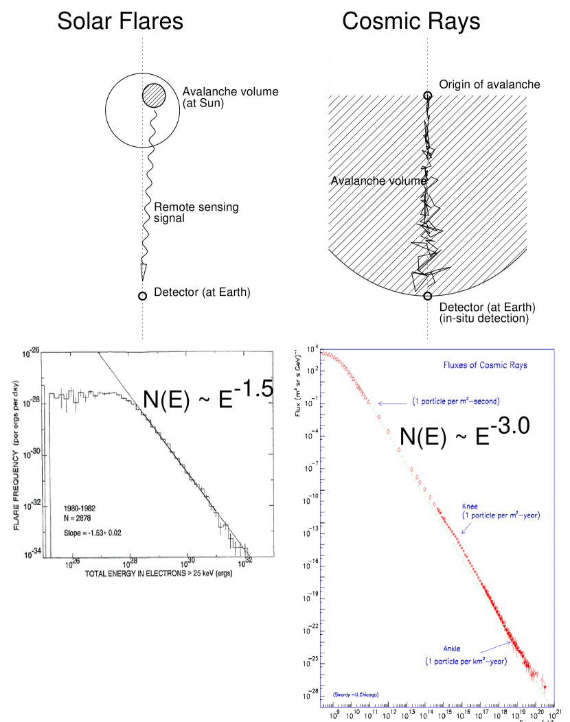
Figure 8: The energy of solar flares is proportional to the avalanche volume, which is probed in its entire 3D volume by remote sensing via soft or hard X-rays (top left), while the energy of cosmic rays detected in-situ is inferred from a linear sub-volume of the entire 3D avalanche only (top right). The predicted energy size distributions are therefore different, with $N(E)\propto E^{-1.5}$ based on the 3D Euclidean volume for solar flares, (bottom left; Crosby et al. 1993), and $N(E)\propto E^{-3.0}$ based on a 1D sub-volume for cosmic rays (bottom right; Credit: Simon Swordy, University of Chicago).

Cosmic rays are high-energetic particles that propagate through a large part of our universe and are accelerated by galactic and extragalactic magnetic fields. Cosmic ray energy spectra span over a huge range of $E=10^{9}-10^{21}$ eV, where the lower limit of $\approx 1$ GeV corresponds to the largest energies that can be accelerated in solar flares and coronal mass ejections. This cosmic ray energy spectrum exhibits an approximate powerlaw function with a mean slope of $\alpha_{E}\approx 3.0$ (Fig. 8, bottom right). A more detailed inspection reveals actually a broken powerlaw with a slope of $\alpha_{E1}\approx 2.7$ below the knee at $E_{knee}\approx 10^{16}$ eV, and a slope of $\alpha_{E2}\approx 3.3$ above the knee. The two energy regimes are associated with the particle origin in galactic space ($E\lower 1.72218pt\hbox{$\;\buildrel<\over{\scriptstyle\sim}\;$}E_{knee}$) and extragalactic space ($E\lower 1.72218pt\hbox{$\;\buildrel>\over{\scriptstyle\sim}\;$}E_{knee})$.

If we interpret a cosmic-ray energy spectrum as a size distribution of particle energies, we can apply our universal SOC model. The driver of the SOC system is a generation mechanism of seed populations of charged particles, which are mostly bound to astrophysical objects in a collisional plasma. A critical threshold is given by transitions of the particles from collisional to collisionless plamsa (such as in the “run-away regime”), where a particle can freely be accelerated, either by Fermi first-order or diffusive shock acceleration. The subsequent particle transport combined with numerous acceleration steps during every passage of suitable electric fields or shock fronts represents the build-up of an avalanche, until the particle hits the Earth’s upper atmosphere where it is detected by a shower of secondary particles. If we could observe all end products of an avalanche, we would expect an energy spectrum of $\alpha_{E}=1.5$. In reality, the energy spectrum of cosmic rays is $\alpha_{E}\approx 3.0$, assuming that the detected energies are proportional to the avalanche volume. How can we explain this discrepancy? A powerlaw index of this value is expected for the size distribution of length scales, $N(L)\propto L^{-3}$ (Eq. 1). Therefore, a similar energy spectrum of $N(E)\propto E^{-3}$ can only be produced if the energy $E$ is proportional to the length scale $L$, requiring that the fractal volume $V_{f}(t)\propto r(t)^{D_{3}}$ has a fractal dimension of $D_{3}=1.0$. Such a scaling can be arranged if only a linear subvolume of an entire 3D avalanche is observed, which is indeed the case for in-situ detection at Earth, since the origin of the cosmic ray avalanche is located far away. The situation is visualized in Fig. 8. In solar flares, on the other hand, almost all energetic particles accelerated during a flare lose their energy in the chromosphere, and thus we can detect the entire energy content of an avalanche event by remote-sensing. This is not possible in cosmic rays, because we cannot detect in-situ all energy losses of cosmic ray particles that originated isotropically from the same avalanche, in a remote place such as in a supernova or black hole. Another aspect that our FD-SOC model predicts is the random walk diffusion during its propagation, which is consistent with the current thinking of cosmic ray particle transport.

Adopting the resulting scaling law between the energy $E$ of a cosmic ray particle and the Euclidian length scale $L$ that a cosmic ray particle has traveled at the time of detection, $E\propto L$, which is expected for direct electric field acceleration in a voltage drop, as well as for any other particle acceleration mechanism with a fixed amount of energy extraction per distance increase, $dE/dL\approx const$, we can even determine the distance to the origination site of the cosmic ray particle. The cosmic ray spectrum shown in Fig. 8 has a knee at $E_{free}\approx 0.5\times 10^{16}$ eV, which marks the distance of the Earth to the center of our galaxy $(L_{gal}\approx 50$ light years or $L_{gal}\approx 5\times 10^{22}$ cm). The Euclidean distance where a cosmic ray particle with a maximum energy of $E_{max}\approx 5\times 10^{20}$ erg originated is then,

$$L_{max}\approx L_{gal}\left({E_{max}\over E_{knee}}\right)\ ,$$ (42)

which yields $L_{max}\approx 5\times 10^{27}$ cm, which corresponds to about 10% of the size of our universe ($R_{uni}\approx 4\times 10^{28}$ cm). Since the intergalactic and extragalactic magnetic fields have different field strengths, the diffusion coefficient of cosmic ray particles is also expected to be different in these two regimes, which may explain the slightly different powerlaw slopes below and above the galactic boundary $L_{gal}$ and the related energy $E_{knee}$.

The lowest energies of the cosmic ray spectrum are at $E_{min}\approx 10^{9}$ eV. Using the same linear scaling of energy with length scale,

$$L_{min}\approx L_{gal}\left({E_{min}\over E_{knee}}\right)\ ,$$ (43)

we estimate a distance of $L_{min}\approx 10^{16}$ cm or 200 AU, which is located somewhat outside of the termination shock of our heliosphere.

5 DISCUSSION

In this paper we developed a macroscopic description of SOC systems that is designed to reproduce the same statistical distributions of observables as from SOC processes occurring on a microscopic level and observed in nature. The microscopic processes cannot be treated analytically due to the large number of degrees of freedom and the nonlinear nature of the dynamic SOC systems. The complexity of the microscopic fine structure during SOC avalanches is captured here in a approximative form by three simple parameters: the fractal dimension $D_{d}$, the diffusion coefficient $\kappa$, and the diffusive spreading exponent $\beta$. What is common to all SOC processes is a system-wide critical threshold level that determines whether “avalanching” occurs or not. For an overview we list the physical mechanisms that operate in SOC systems in Table 2, containing a few classical SOC systems, as well as astrophysical applications that we described in this paper. We are aware that we use the term “self-organized criticality” in a more general sense than originally envisioned, in the spirit of the definition given in the introduction: SOC is a critical state of a nonlinear energy dissipation system that is slowly and continuously driven towards a critical value of a system-wide instability threshold, producing scale-free, fractal-diffusive, and intermittent avalanches with powerlaw-like size distributions.

Let us discuss the meaning of self-organizing criticality in astrophysical applications in some more detail. Essentially we have three aspects of a SOC system: (1) the energy input of the slow and steady driver, (2) the self-organizing criticality condition or instability threshold, and (3) the energy output in form of intermittent avalanches (Table 2). The driver is necessary to keep a SOC process going, because the SOC process would stop otherwise as soon as the system becomes subcritical. The instability threshold $z_{crit}$ represents a bifurcation of two possible dynamic outcomes: either nothing happens when the state in every node of a SOC system is below this critical threshold ($z<z_{crit}$), while an avalanche or nonlinear energy dissipation event is triggered when a threshold exceeds at some location ($z\geq z_{crit}$). In classical SOC systems, the self-organizing threshold can be a critical slope or angle of repose (sandpile), a phase transition point (superconductor, Ising model, tea kettle), a fire ignition threshold (forest fires), or dynamic friction (earthquakes). In astrophysical systems, the instability thresholds or critical values are equally diverse, such as thresholds for magnetic instability with subsequent magnetic reconnection (magnetospheric substorms, solar flares, stellar flares), magnetic stressing (neutron star quakes, accretion disk flares), particle acceleration thresholds, such as the “run-away regime” (solar energetic particles, cosmic rays), vortex unpinning (neutron stars), critical mass density for accretion (planetesimals, asteroids, accretion disk flares, black-hole objects), gravitational disturbances and unstable orbits that trigger collisions (Saturn ring particles, lunar craters), etc. All these instability thresholds have system-wide critical values, so that nothing happens below those values, while avalanching happens above their value. Since these instability thresholds or critical values occur system-wide, set by physical conditions of the internal microscopic processes, the system is self-organizing or self-tuning in the sense that it maintains the same critical values throughout the system. This follows the basic philosophy of Bak’s sandpile, where a critical slope is maintained system-wide, internally given by the critical value where the gravitational and the dynamic friction forces are matching. For magnetic reconnection processes, for instance, critical values are given by the kink-instability criterion or by the torus instability criterion. For the formation of planetesimals (as well as for the formation of planets and stars), a critical mass density is required where accretion by self-gravity overcomes diffusion. Thus, all these astrophysical processes fulfill the basic requirement of our SOC definition, i.e., these nonlinear systems are slowly driven towards a critical value of a system-wide instability threshold. And all of these astrophysical processes exhibit scale-free, fractal-diffuse, and intermittent avalanches, with powerlaw-like size distributions.

6 CONCLUSIONS

We can summarize the conclusions of this study as follows:

1. We propose the following general definition of a SOC system: SOC is a critical state of a nonlinear energy dissipation system that is slowly and continuously driven towards a critical value of a system-wide instability threshold, producing scale-free, fractal-diffusive, and intermittent avalanches with powerlaw-like size distributions. This generalized definition expands the original meaning of self-tuning “criticality” to a wider class of critical points and instability thresholds that have a similar (nonlinear) dynamical behavior and produce similar (powerlaw-like) statistical size distributions.

2. A macroscopic description of SOC systems has been derived from first principles that predicts powerlaw functions for the size distributions of SOC parameters, as well as universal values of the powerlaw slopes, for geometric and temporal parameters, and some observables (flux and energy if they are proportional to the emitting fractal volume). This macroscopic SOC model exhibits powerlaw scaling, universality, spatio-temporal correlations, separation of time scales, fractality, and intermittency. The predicted powerlaw slopes depend only on three parameters: on the Euclidean dimension $d$ of the system, the fractal dimension $D_{d}$, and the diffusive spreading exponent $\beta$. Note, that the spreading exponent is an adjustable parameter in the FD-SOC model and can accomodate classical diffusion, sub-diffusive, or hyper-diffusive transport, and thus represents in some sense an ordering parameter, while it cannot be adjusted in a branching process or in a BTW model with a given re-distribution rule.

3. The FD-SOC model makes the following predictions: For the case of 3D space ($d=3$) and classical diffusion ($\beta=1$), the predicted values for the average fractal dimension is $D_{d}\approx(1+d)/3=2$, the powerlaw slopes are $\alpha_{L}=3$ for length scales, $\alpha_{T}=2$ for time scales, $\alpha_{F}=2$ for fluxes or energy dissipation rates, $\alpha_{P}=5/3$ for peak fluxes or peak energy dissipation rates, and $\alpha_{E}=3/2$ for fluences (i.e., time-integrated fluxes) or (total) avalanche energies, assuming proportionality between the time-integrated fractal avalanche volume and the observed fluence.

4. Among the astrophysical applications we find agreement between the predicted and observed size distributions for the following phenomena: lunar craters, asteroid belts, Saturn ring particles, auroral events during magnetospheric substorms, outer radiation belt electron bursts, solar flares, soft gamma-ray repeaters, and blazars. This agreement between theory and observations supports the universal applicability of the fractal-diffusive SOC model.

5. Discrepancies between the predicted and observed size distributions are found for stellar flares, pulsar glitches, black holes, and cosmic rays, but some can be reconciled with modified SOC models. The disagreement for solar energetic particle (SEP) events is believed to be due to a selection bias for large events. For stellar flares we conclude that the bolometric fluence is not proportional to the dissipated energy and volume. Pulsar glitches are subject to small-number statistics. Black hole pulses have extremely steep size distributions that could be explained by a suppression of large pulses for a certain period after a large pulse. For cosmic rays, the energy size distribution implies a fractal dimension of $D_{3}=1$ and a proportionality between energy and length scales ($E\propto L$) according to our FD-SOC model, which can be explained by the nature of in-situ detections that capture only a small fraction of the avalanche volume.

Whatever the correct interpretations are for those phenomena with unexpected size distributions, the application of our standard FD-SOC model can reveal alternative scaling laws that can be tested in future measurements. A major achievement of our standard FD-SOC model is the fact that it can predict and explain, in a universal way, the powerlaw indices of different SOC parameters (lengths, durations, fluxes, energies, waiting times) in most of the considered astrophysical applications, which do not depend on the details of the underlying physical mechanisms. We have also to appreciate that the macroscopic approach of SOC statistics does not depend on the microscopic fine structure of each SOC process, unlike the mathematical/numerical SOC models, which produce different powerlaw slopes depending on the assumed re-distribution rule, and partially do not fulfill universality. Our macroscopic fractal-diffusive SOC model may also be suitable to correctly describe the statistics of other, SOC-related, nonlinear processes, such as percolation or turbulence, an aspect that needs to be investigated in future.

Table 1: Summary of theoretically predicted and observed powerlaw indices of size distributions in astrophysical systems.

	Length	Area	Duration	Peak flux	Energy	Waiting
	$\alpha_{L}$	$\alpha_{A}$, $\alpha_{th,A}$	$\alpha_{T}$	$\alpha_{P}$	$\alpha_{E}$	time $\alpha_{\Delta t}$
FD-SOC Theory	3.0	2.0	2.0	1.67	1.5	2.0
Lunar craters:
Mare Tranquillitatis ${}^{1})$	3.0
Meteorites and debris ${}^{2})$	2.75
Asteroid belt:
Spacewatch Surveys${}^{3})$	2.8
Sloan Survey${}^{4})$	2.3-4.0
Subaru Survey${}^{5})$	2.3
Saturn ring:
Voyager 1${}^{6})$	2.74-3.11
Magnetosphere:
EUV auroral events7		1.73$-$1.92	2.08$-$2.39	1.66$-$1.82	1.39$-$1.61
Optical auroral events8		1.85$-$1.98	2.25$-$2.53	1.71$-$2.02	1.50$-$1.74
Outer radiation belt${}^{9})$				1.5$-$2.1
Solar Flares:
HXR, ISEE-310			1.88-2.73	1.75-1.86	1.51-1.62
HXR, HXRBS/SMM11			$2.17\pm 0.05$	$1.73\pm 0.01$	$1.53\pm 0.02$	2.0a
HXR, BATSE/CGRO12			2.20-2.42	1.67-1.69	1.56-1.58	2.14$\pm$0.01b
HXR, RHESSI13			1.8-2.2	1.58-1.77	1.65-1.77	2.0a
SXR, Yohkoh14	1.96$-$2.41	1.77-1.94		1.64-1.89	1.4-1.6
SXR, GOES15			2.0-5.0	1.86-1.98	1.88	1.8$-$2.4c
EUV, SOHO/EIT16		2.3-2.6	1.4-2.0
EUV, TRACE17	2.50$-$2.75	2.4-2.6		1.52-2.35	1.41-2.06
EUV, AIA/SDO18	3.2$\pm$0.7	$2.1\pm 0.3$	$2.10\pm 0.18$	$2.0\pm 0.1$	$1.6\pm 0.2$
EUV, EIT/SOHO19	3.15$\pm$0.18	2.52$\pm$0.05	1.79$\pm$0.03		1.48$\pm$0.03
Magnetic events, MDI/SOHO19	2.57$\pm$0.13	1.93$\pm$0.06	2.02$\pm$0.07		1.47$\pm$0.03
Radio microwave bursts20				1.2-2.5
Radio type III bursts21				1.26-1.91
Solar energetic particles22				1.10-2.42	1.27-1.32
Stellar Flares:
EUVE flare stars23					$2.17\pm 0.25$
KEPLER flare stars24				$1.88\pm 0.09$	$2.04\pm 0.13$
Astrophysical Objects:
Crab pulsar25				3.06-3.50
PSR B1937+2126				$2.8\pm 0.1$
Soft Gamma-Ray repeaters27					$1.43-1.76$
Cygnus X-1 black hole28				7.1
Blazar GC 0109+22429				1.55
Cosmic rays30					$2.7-3.3$

References to Table 13.2: ${}^{1})$ Cross (1966); ${}^{2})$ Sornette (2004); ${}^{3})$ Jedicke and Metcalfe (1998); ${}^{4})$ Ivezic et al. (2001); ${}^{5})$ Yoshida et al. (2003), Yoshida and Nakamura (2007); ${}^{6})$ Zebker et al. (1985), French and Nicholson (2000); ${}^{7})$ Uritsky et al. (2002); ${}^{8})$ Kozelov et al. (2004); ${}^{9})$ Crosby et al. (2005) ${}^{10})$ Lu et al. (1993), Lee et al. (1993); ${}^{11})$ Crosby et al. (1993); ${}^{12})$ Aschwanden  (2012a,2011b); ${}^{13})$ Christe et al. (2008), Lin et al. (2001), Aschwanden  (2011a,c); ${}^{14})$ Shimizu (1995), Aschwanden and Parnell (2002); ${}^{15})$ Lee et al. (1995), Feldman et al. (1997), Veronig et al. (2002a,b), Aschwanden and Freeland (2012); ${}^{16})$ Krucker and Benz (1998), McIntosh and Gurman (2005); ${}^{17})$ Parnell and Jupp (2000), Aschwanden et al. 2000, Benz and Krucker (2002), Aschwanden and Parnell (2002), Georgoulis et al. (2002); ${}^{18})$ Aschwanden and Shimizu (2013), Aschwanden, Zhang, and Liu (2013); ¹⁹ Uritsky et al. (2002); ${}^{20})$ Akabane (1956), Kundu (1965), Kakinuma et al. (1969), Das et al. (1997), Nita et al. (2002); ${}^{21})$ Fitzenreiter et al. (1976), Aschwanden et al. (1995), Das et al. (1997), Nita et al. (2002); ${}^{22})$ Van Hollebeke et al. (1975), Belovsky and Ochelkov (1979), Cliver et al. (1991), Gabriel and Feynman (1996), Smart and Shea (1997), Mendoza et al. (1997), Miroshnichenko et al. (2001), Gerontidou et al. (2002); Gabriel and Feynman (1996); ${}^{23})$ Robinson et al. (1999). Audard et al. (2000), Kashyap et al. (2002), Güdel et al. (2003), Arzner and Güdel (2004), Arzner et al. (2007), Stelzer et al. (2007); ${}^{24})$ Maehara et al. 2012; Shibayama et al. 2013; ${}^{25})$ Argyle and Gower (1972), Lundgren et al. (1995); ${}^{26})$ Cognard et al. (1996); ${}^{27})$ Gogus et al. (1999, 2000); ${}^{28})$ Negoro et al. (1995), Mineshige and Negoro (1999); ${}^{29})$ Ciprini et al. (2003); ${}^{30})$ e.g., Fig. 13.18 (courtesy of Simon Swordy, Univ.Chicago); ${}^{a})$ Aschwanden and McTiernan (2010); ${}^{b})$ Grigolini et al. (2002); ${}^{c})$ Wheatland (2001, 2003), Boffetta et al. (1999), Lepreti et al. (2001).

Table 2: Physical mechanisms operating in self-organized criticality systems.

Phenomenon	Energy Input	Instability threshold	Energy output
	(steady driver)	(criticality)	(intermittent avalanches)
CLASSICAL SOC:
Sandpile	gravity (dripping sand)	angle of repose	sand avalanches
Superconductor	magnetic field change	phase transition	vortex avalanches
Ising model	temperature increase	phase transition	atomic spin-flip
Tea kettle	temperature increase	boiling point	vapour bubbles
Earthquakes	tectonic stressing	dynamical friction	rupture area
Forest fire	tree growth	fire ignition point	burned area
BTW cellular automaton	input at random nodes	critical threshold	next-neighbor redistribution
ASTROPHYSICS:
Lunar craters	meteorite production	lunar collision	lunar impact craters
Asteroid belt	planetesimals	critical mass density	asteroids
Saturn ring	gravitational disturbances	collision rate	Saturn ring particles
Magnetospheric substorm	solar wind	magnetic reconnection	auroral bursts
Radiation belt	solar wind	magnetic trapping/untrapping	electron bursts
Solar flares	magnetic stressing	magnetic reconnection	nonthermal particles
Stellar flares	magnetic stressing	magnetic reconnection	nonthermal particles
Pulsar glitches	neutron star spin-up	vortex unpinning	neutron starquakes
Soft gamma-ray repeaters	magnetic stressing	star crust fracture	neutron starquakes
Black-hole objects	gravity	accretion and inflow	X-ray bremsstrahlung pulses
Blazars	quasar jets	jet direction jitter	optical radiation pulses
Cosmic rays	galactic magnetic fields	(run-away) acceleration threshold	high-energy particles

Figure 3: The spatio-temporal evolution of the avalanche radius $r(t)$ is shown (top panel), the expansion velocity $v(t)$ (second panel), the energy dissipation rate or flux $F(t)$ (third panel), and the dissipated energy $E(t)$ (bottom panel), are shown for our macroscopic FD-SOC model for diffusive spreading exponents of $\beta=0.1$ (quasi-logistic; solid line style), $\beta=0.5$ (sub-diffusive; dashed line style), and $\beta=1$ (classical diffusion, solid line style).

Figure 7: The scaling law of the total solar irradiance (TSI) and the GOES 1-8 Å peak flux based on a linear regression fit (solid line) to data from Kretzschmar (2011) is shown, i.e., $E_{b}\propto P_{x}^{0.78\pm 0.13}$ (top panel). A linear relationship is indicated with a dotted line. The bolometric flare energy of 1538 stellar flares observed with Kepler is histogrammed, yielding a size distribution with a powerlaw slope of $\alpha_{E}=2.04\pm 0.13$ (middle panel), and the inferred size distribution of GOES fluxes using the scaling law of Kretzschmar (2011), yielding a powerlaw slope of $\alpha_{P}=1.88\pm 0.09$ (bottom panel).

References

- (1)
- (2) Akabane, K. 1956, Publ. Astron. Soc. Japan 8, 173.
- (3) Angelopoulos, V., Mukai, V., and Kobukun, S. 1999, Phys. Plasmas 6/11, 4161.
- (4) Argyle, E. and Gower, J.F.R. 1972, ApJ 175, L89.
- (5) Arzner, K. and Güdel, M. 2004, ApJ 602, 363.
- (6) Arzner, K., Güdel, M., Briggs, K., Telleschi, A. and Audard, M. 2007, A&A 468, 477.
- (7) Aschwanden, M.J., Benz, A.O., Dennis, B.R., and Schwartz, R.A. 1995, ApJ 455, 347.
- (8) Aschwanden, M.J., Tarbell, T., Nightingale, R., Schrijver, C.J., Title, A., Kankelborg, C.C., Martens, P.C.H., and Warren,H.P. 2000, ApJ 535, 1047.
- (9) Aschwanden, M.J., and Parnell,C.E. 2002, ApJ, 572, 1048.
- (10) Aschwanden, M.J. and McTiernan, J.M. 2010, ApJ 717, 683.
- (11) Aschwanden, M.J. 2011a, Self-Organized Criticality in Astrophysics. The Statistics of Nonlinear Processes in the Universe, Springer-Praxis: Heidelberg, New York, 416p.
- (12) Aschwanden, M.J. 2011b, Solar Phys. 274, 99.
- (13) Aschwanden, M.J. 2012a, A&A, 539, A2.
- (14) Aschwanden, M.J. 2012b, ApJ, 757, 94.
- (15) Aschwanden, M.J. and Freeland, S.L. 2012, ApJ, 754, 112.
- (16) Aschwanden, M.J. (Ed.) 2013, “Self-Organized Criticality Systems”, Open Academic Press, Warsaw, Berlin; http://www.openacademicpress.de/, 483pp.
- (17) Aschwanden, M.J., Zhang, J., and Liu,K. 2013, ApJ, 775, 23.
- (18) Aschwanden, M.J. and Shimizu, T. 2013, ApJ, 776, 132.
- (19) Audard, M., Güdel, M., Drake, J.J., and Kashyap, V.L. 2000, ApJ 541, 396.
- (20) Bak, P., Tang, C., and Wiesenfeld, K. 1987, PhRvL 59/4, 381.
- (21) Bak, P., Tang, C., and Wiesenfeld, K. 1988, PhRvA 38, 364.
- (22) Bak, P., and Chen, K. 1989, JPhD 38, 5.
- (23) Barabasi, A.L. and Stanley, H.E. 1995, Fractal Concepts in Surface Growth, Cambridge: Cambridge University Press.
- (24) Belovsky, M.N. and Ochelkov, Yu. P. 1979, Izvestiya AN SSR, Phys. Ser. 43, 749.
- (25) Benz, A.O. and Krucker, S. 2002, ApJ, 568, 413.
- (26) Biham, O., Milshtein, E., and Ofer, M. 2001, Phys.Rev. E 63(6), 061309.
- (27) Boffetta, G., Carbone, V., Giuliani, P., Veltri, P., and Vulpiani, A. 1999, Phys. Rev. Lett. 83/2, 4662.
- (28) Botke, W.F., Durda, D.D., Nesvorny, D., Jedicke,R., Morbidelli, A., Vokrouhlicky, D. 2005, Icarus, 175, 111.
- (29) Chapman, S.C. and Watkins, N. 2001, SSRv 95, 293.
- (30) Charbonneau, P., McIntosh, S.W., Liu, H.L., and Bodgan, T. 2001, Solar Phys. 203, 321.
- (31) Christe, S., Hannah, I.G., Krucker, S., McTiernan, J., and Lin, R.P. 2008, ApJ 677, 1385.
- (32) Christensen, K. and Moloney, N.R. 2005, Complexity and Criticality, London: Imperial College Press.
- (33) Ciprini,S., Fiorucci, M., Tosti, G., and Marchili, N. 2003, Astron. Soc. Pacific Conf. Ser. 299, 265.
- (34) Cliver, E.W., Ling, A.G., Belov, A., and Yashiro, S. 2012, ApJ 756, L29.
- (35) Cliver, E., Reames, D., Kahler, S., and Cane, H. 1991, Internat. Cosmic Ray Conf. 22nd Dublin, LEAC A92-36806 15-93, NASA: Greenbelt, p.2, 1-4
- (36) Cognard, I., Shrauner, J.A., Taylor, J.H., and Thorsett, S.E. 1996, ApJ 457, L81.
- (37) Craig, I.J.D. 2001, Solar Phys. 202, 109.
- (38) Crosby, N.B., Aschwanden, M.J., and Dennis, B.R. 1993, Sol. Phys., 143, 275.
- (39) Crosby, N.B., Meredith, N.P., Coates, A.J., and Iles, R.H.A. 2005, Processes in Geophysics 12, 993.
- (40) Cross, C.A. 1966, MNRAS 134, 245.
- (41) Das, T.K., Tarafdar, G., and Sen, A.K. 1997, Solar Phys. 176, 181.
- (42) Erzan, A., Pietronero, L., and Vespignani, A. 1995, Rev. Mod. Phys. 67(3), 545.
- (43) Feder, H.J. and Fecer J. 1991, Phys. Rev. Lett. 66, 2669.
- (44) Feldman, U., Doschek, G.A., and Klimchuk, J.A. 1997, ApJ 474, 511.
- (45) Fitzenreiter, R.J., Fainberg, J., and Bundy, R.B. 1976, Solar Phys. 46, 465.
- (46) Foster, D, Nelson, D.R., and Stephen, M.J. 1977, Physl. Rev. A 16(2), 732.
- (47) Freeman, M.P., Watkins, N.W., and Riley, D.J. 2000, GRL 27, 1087.
- (48) French, R.G. and Nicholson, P.D. 2000, Icarus 145, 502.
- (49) Gabriel, S.B. and Feynman, J. 1996, Solar Phys. 165, 337.
- (50) Georgoulis, M.K., Rust, D.V., Bernasconi, P.N., and Schmieder, B. 2002, ApJ 575, 506.
- (51) Gerontidou, M., Vassila,i, A., Mavromichalaki, H., and Kurt, V. 2002, J. Atmos. Solar-Terr. Phys. 64(5-6), 489.
- (52) Gogus E., Woods,P.M., Kouveliotou,C., Van Paradijs,J., Briggs, M.S., Duncan, R.C. and Thompson, C. 1999, ApJ 526, L93.
- (53) Gogus, E., Woods, P.M., Kouveliotou, C., van Paradijs, J., Briggs, M.S., Duncan, R.C., and Thompson, C. 2000, ApJ 532, L121.
- (54) Grassberger, P., and De la Torre, A. 1979, Ann. Phys. 122(2), 373.
- (55) Grigolini, P., Leddon, D., and Scafetta, N. 2002, Phys. Rev. E 65, 046203.
- (56) Güdel, M., Audard, M., Kashyap, V.L., and Guinan, E.F. 2003, ApJ 582, 423.
- (57) Gutenberg, B. and Richer, C.F. 1949, Seismicity of the Earth, Princeton, NJ: Princetorn University Press.
- (58) Held, G.A., Solina, D.H., Solina, H., Keane, D.T., Haag, W.J., Horn, P.M., and Grinstein, G. 1990, Phys. Rev. Lett. 65, 1120.
- (59) Ising, E. 1925, Z. Phys. 31, 253.
- (60) Ito, K. and Matsuzaki M. 1990, JGR 95(B5), 6853.
- (61) Ivanov, B.A. 2001, SSRv 96, 1/4, 87.
- (62) Ivecik, Z., Tabachnik, S., Rafikov, R., Lupton, R.H., Quinn, T., Hammergren, M., Eyer, L., Chu, J., et al. 2001, AJ 122, 2749.
- (63) Jedicke, R. and Metcalfe, T.S. 1998, Icarus 131(2), 245.
- (64) Jensen, H.J. 1998, Self-Organized Criticality, Emergent complex behavior in physical and biological systems, Cambridge: Cambridge University Press.
- (65) Kahler, S.W. 2013, ApJ 769, 35, 5pp.
- (66) Kakinuma, T., Yamashita, T., and Enome, S. 1969, Proc. Res. Inst. Atmos. Nagoya Univ., Japan, 16, 127.
- (67) Kashyap, V.L., Drake, J.J., Güdel, M., and Audard, M. 2002, ApJ 580, 1118.
- (68) Klimas, A.J., Uritsky, V.M., and Donovan, E. 2010, JGRA 115, A06202.
- (69) Kouveliotou, C., Dieters, S., Strohmayer, T., van Paradijs, J., Fishman, G.J., Meegan, C.A., Hurley, K., Kommers, J., et al. 1998, Nature 393, 235.
- (70) Kouveliotou, C., Strohmayer, T., Hurley, K., van Paradijs, J., Finger, M.H., Dieters, S., Woods, P., Thomson, C. and Duncan, R.C. 1999, ApJ 510, L115.
- (71) Kozelov, B.V., Uritsky, V.M., and Klimas, A.J. 2004, JGR 31, L20804.
- (72) Kretzschmar, M. 2011, A&A 530, A84.
- (73) Kucera, T.A., Dennis, B.R., Schwartz, R.A., and Shaw, D. 1997, ApJ 475, 338.
- (74) Krucker, S. and Benz, A.O. 1998, ApJ 501, L213.
- (75) Kundu, M.R. 1965, Solar Radio Astronomy, Interscience Publication: New York, 660p.
- (76) Lawrence, J.K. 1991, Solar Phys. 135, 249.
- (77) Lawrence, J.K. and Schrijver, C.J. 1993, ApJ 411, 402.
- (78) Lee, T.T., Petrosian,V., and McTiernan, J.M. 1993, ApJ 412, 401.
- (79) Lee, T.T., Petrosian,V., and McTiernan, J.M. 1995, ApJ 418, 915.
- (80) Lepreti, F., Fanello, P.C., Zaccaro, F., and Carbone, V. 2000, Solar Phys. 197, 149.
- (81) Lin, R.P, Feffer, P.T., and Schwartz, R.A. 2001, ApJ 557, L125.
- (82) Liu, H.L., Charbonneau, P., Bogdan, T.J., Poquet, A., and McIntosh, S.W. 2001, Phys. Rev. E 66, 056111.
- (83) Longcope, D.W. and Sudan, R.N. 1992, Ph.Rev.Lett. 68(11), 1706.
- (84) Lu, E.T. and Hamilton, R.J. 1991, ApJ 380, L89.
- (85) Lu, E.T., Hamilton, R.J., McTiernan, J.M., and Bromund, K.R. 1993, Ap 412, 841.
- (86) Lui, A.T.Y., Chapman, S.C., Liou,K., Newell, P.T., Meng, C.I., Brittnacher, M., and Parks, G.K. 2000, GRL 27/7, 911.
- (87) Lundgren, S.C., Cordes, J.M., Ulmer, M., Matz, S.M., Lomatch, S., Foster, R.S., and Hankins, T. 1995, ApJ 453, 433.
- (88) McAteer, R.T.J. 2013, in ”Self-Organized Criticality Systems” (ed. Aschwanden,M.J.), Open Academic Press GmbH & Co., http://www.openacademicpress.de.
- (89) Maehara, H., Shibayama, T., Notsu, S., Notsu, Y., Nagao, T., Kusaba, S., Honda, S., Nogami, D., and Shibata, K. 2012, Nature 485, 478.
- (90) Main, I.G. and Burton, P.W. 1984, Bull. Seismolog. Soc. America 74, 1409.
- (91) Mandelbrot, B.B. 1977, Fractals: form, chance, and dimension, Translation of Les objects fractals, W.H. Freeman, San Francisco.
- (92) Mandelbrot, B.B. 1983, The fractal geometry of nature, W.H. Freeman, San Francisco.
- (93) Mandelbrot, B.B. 1985, Self-affine fractals and fractal dimension, Physica Scripta 32, 257-260.
- (94) McIntosh, S.W., Charbonneau, P., Bogdan, T.J., Liu, H., and Norman, J.P. 2002, Phys. Rev. Lett. 65 046125.
- (95) Medina, E., Hua, T., Kardar, M., and Zhang, Y.C. 1989, Phys. Rev. A 39(6), 3053.
- (96) Melatos, A., Peralta, C., and Wyithe, J.S.B. 2008, ApJ 672, 1103.
- (97) McIntosh, S.W. and Gurman, J.B. 2005, Solar Phys. 228, 285.
- (98) Mendoza, B., Melendez-Venancio, R., Miroshnichenko, L.I., and Perez-Enriquez, R. 1997, in Proc. 25th Int. Cosmic Ray Conf., 1, 81.
- (99) Mineshige, S. and Negoro, H. 1999, ASP Conf. Ser. 161, 113.
- (100) Miroshnichenko, L.I., Mendoza, B., and Perez-Enriquez, R. 2001, Solar Phys. 202, 151.
- (101) Munoz, M.A., Dickman, R., Cespignani, A., and Zapperi S. 1999, Phys. Rev. E, 59, 6175.
- (102) Neukum, G., Ivanov, B.A., and Hartmann, W.K. 2001, SSRv 96, 1/4, 55.
- (103) Negoro, H., Kitamoto, S., Takeuchi, M., and Mineshige, S. 1995, ApJ 452, L49.
- (104) Nita, G.M., Gary, D.R., Lanzerotti, L.J., and Thomson, D.J. 2002, ApJ 570, 423.
- (105) Notsu, Y., Shibayama, T., Maehara, H., Notsu, S., Nagao, T., Honda, S., Ishii, T.T., Nogami, D., and Shibata, K. 2013, ApJ 771, 127.
- (106) Parnell, C.E., and Jupp, P.E. 2000, ApJ529, 554.
- (107) Pruessner, G. 2012, Self-Organised Criticality, Cambridge: Cambridge University Press.
- (108) Richter, C.F. 1958, Elementary Seismology, W.H. Freeman, San Francisco, California.
- (109) Rinaldo, A., Rodriguez-Iturbe, I., Rigon, R., Ijjasz-Vasquez, E., and Bras, R.L. 1993, Phys. Rev. Lett. 70(6), 822.
- (110) Robinson, P.A. 1994, Phys.Rev. E 49(5), 3919.
- (111) Robinson, R.D., Carpenter, K.G., and Percival, J.W. 1999, ApJ 516, 916.
- (112) Rosner, R., Tucker, W.H., and Vaiana, G.S. 1978, ApJ, 220, 643.
- (113) Schrijver, C.J., Sandman, A.W., Aschwanden, M.J., and DeRosa, M.L. 2004, ApJ 615, 512.
- (114) Shimizu, T. 1995, Publ. Astron. Soc. Japan 47, 251.
- (115) Shibayama, T., Maehara, H., Notsu, S., Notsu, Y., Nagao, T., Honda, S., Ishii, T.T., Nogami, D., and Shibata, K. 2013, ApJSS 209, 5.
- (116) Sethna, J.P., Dahmen, K.A¿, and Myers, C.R. 2001, Nature 410(6825), 242.
- (117) Smart, D.F. and Shea, M.A. 1997, in Proc. Solar-Terrestrial Prediction Workshop V, Hiraiso Solar-Terrestrial Research Center, Japan, p.449.
- (118) Sornette, D. 2004, Critical phenomena in natural sciences: chaos, fractals, self-organization and disorder: concepts and tools, Springer, Heidelberg, 528 p.
- (119) Stelzer, B., Flaccomio, E., Briggs, K., Micela, G., Scelsi, L., Audard, M., Pillitteri, I. and Güdel, M. 2007, ApJ 468, 463.
- (120) Takalo, J. 1993, Ph. Lic. Thesis, University of Jyväskylä.
- (121) Takalo, J., Timonem, J., Klimas, A., Valdivia, J., and Vassiliadis, D. 1999, GRL 26/13, 1813.
- (122) Takeuchi, M., Mineshige, S., and Negoro, H. 1995, Publ. Astron. Soc. Japan 47, 617.
- (123) Telloni, D., Carbone, V., Lepreti, F., and Antonucci, E. 2014, Astrophys. J. Lett. (in press).
- (124) Thompson, C. and Duncan, R.C. 1996, ApJ 473, 322.
- (125) Uritsky, V.M., Pudovkin, M.I., Steen, A. 2001, JASTP 63 (13), 1415.
- (126) Uritsky, V.M., Klimas, A.J., Vassiliadis, D., Chua, D., and Parks, G. 2002, JGR 107, A12, 1426.
- (127) Uritsky, V.M., Klimas, A.J., and Vassiliadis, D. 2006, GRL 33, L08102.
- (128) Uritsky, V.M., Davila, J.M., Ofman, L., and Coyner, A.J. 2013, ApJ 769, 62.
- (129) Van Hollebeke, M.A.I., Ma Sung, L.S., and McDonald F.B. 1975, Solar Phys. 41. 189.
- (130) Van Houten, C.J., can Houten-Groeneveld, I., Herget, P., and Gehrels, T. 1970, AApSS 2/5, 339.
- (131) Vespignani, A., and Zapperi, S. 1998, Phys. Rev. E 57, 6345.
- (132) Veronig, A., Temmer, M., Hanslmeier, A., Otruba, W., and Messerotti, M. 2002a, A&A 382, 1070.
- (133) Veronig, A., Temmer, M., and Hanslmeier, A. 2002b, Hvar Obs. Bull. 26/1, 7.
- (134) Walkowicz, L.M.,Basri, G., Batalha, N., Gilliland, R.L., Jenkins, J., Borucki, W.J., Koch, D., Caldwll, D., et al. 2011, ApJ 141, 50.
- (135) Warzawski, L. and Melatos, A. 2008, MNRAS 390/1, 175..
- (136) Wheatland, M.S. 2001, Solar Phys. 203, 87.
- (137) Wheatland, M.S. 2003, Solar Phys. 214, 361.
- (138) Wiesenfeld, K., Tang, C., and Bak, P. 1989, J. Stat. Phys. 54, 1441.
- (139) Yoshida, F., Nakamura, T., Watanabe. J., Kinoshita, D., and Yamamoto, N. 2003, Publ. Astron. Soc. Japan 55, 701.
- (140) Yoshida, F. and Nakamura, T. 2007, Planet. Space Science 55, 113.
- (141) Young, M.D.T. and Kenny, B.G. 1996, ASP COnf. Ser. 105 (eds. Johnston, S., Walker, M.A., and Bailes, M.), ASP: San Francisco, p179.
- (142) Zebker, H.A., Marouf, E.A., and Tyler, G.L. 1985, Icarus 64, 531.
- (143) Zhang, Y.C. 1989, Phys. Rev. Lett. 63(5), 470.
- (144)