The Gemini NICI Planet-Finding Campaign:
The Companion Detection Pipeline.

Abstract

We present the high-contrast image processing techniques used by the Gemini NICI Planet-Finding Campaign to detect faint companions to bright stars. NICI (Near Infrared Coronagraphic Imager) is an adaptive optics instrument installed on the 8-m Gemini South telescope, capable of angular and spectral difference imaging and specificially designed to image exoplanets. The Campaign data pipeline achieves median contrasts of 12.6 magnitudes at 0.5^′′ and 14.4 magnitudes at 1^′′ separation, for a sample of 45 stars ($V=$ 4.3–13.9 mag) from the early phase of the Campaign. We also present a novel approach to calculating contrast curves for companion detection based on 95% completeness in the recovery of artificial companions injected into the raw data, while accounting for the false-positive rate. We use this technique to select the image processing algorithms that are more successful at recovering faint simulated point sources. We compare our pipeline to the performance of the LOCI algorithm for NICI data and do not find significant improvement with LOCI.

1 INTRODUCTION

The study of exoplanets has advanced admirably in the last two decades, through the application of radial velocity, transit and microlensing techniques (e.g., Marcy et al., 2008; Borucki et al., 2010; Gould et al., 2010). Over 800 exoplanet detections have placed significant constraints on the mass and separation distribution of exoplanets for separations $\lesssim$3 AU from their parent stars (e.g., Cumming et al., 2008; Howard et al., 2010).

In comparison, current direct imaging techniques can detect Jupiter-mass planets at separations beyond $\sim$10 AU from the host star. Moreover, detecting photons from exoplanets allows us to study their atmospheres spectroscopically (e.g., Bowler et al., 2010; Barman et al., 2011). Several extrasolar planets have been directly imaged, including (1) HR 8799 bcde, a system with 4 massive (4–10 $M_{Jup}$) planets (Marois et al., 2008, 2010b); (2) $\beta$ Pictoris b, a 8${}^{+5}_{-2}$ $M_{Jup}$ planet first detected at only 3 AU separation from its primary star (Lagrange et al., 2009, 2010); (3) Fomalhaut b, a planet with a possible circum-planetary disk detected at 115 AU from the host star (Kalas et al., 2008, 2013); (4)  1RXS J1609$-$2105 b, an 8$\pm$3$M_{Jup}$ planet around a 5 Myr old star in the Upper Scorpius Association (Lafrenière et al., 2008; Lafreniere et al., 2010); (5) HD 95086 b, a 4–5$M_{Jup}$ planet around 10–17 Myr old A8 star (Rameau et al., 2013; Meshkat et al., 2013); (6) GJ 504 b, a 4–9$M_{Jup}$ planet around a 100-500 Myr old Sun-like star (Kuzuhara et al., 2013; Janson et al., 2013).

In recent years, several challenges have been overcome in the field of direct imaging. To achieve high sensitivity to point sources at sub-arcsecond separations, the intensity of the stellar halo can now be significantly reduced using adaptive optics (AO) and a coronagraph. However, long-lived speckles still dominate at angular separations close to the star in AO images and are difficult to distinguish from astronomical point sources. In addition, an impressive variety of instrumental and post-processing techniques have been developed to reduce the effect of these speckles. For example, angular differential imaging (ADI; Liu, 2004; Marois et al., 2005) decouples the sky rotation of the planet from the speckles. Spectral differencing imaging (SDI; Racine et al., 1999) and spectral deconvolution (Sparks & Ford, 2002; Thatte et al., 2007) help distinguish between the star and planet, taking advantage of the different ways their fluxes change as a function of wavelength. Finally, the study of speckle statistics over time can help to distinguish planets from speckles over multiple exposures (Gladysz & Christou, 2009).

Several direct imaging AO surveys of young ($\lesssim$100 Myr old) stars have been completed over the past decade. These have placed increasingly stronger constraints on the population of substellar companions and giant planets around nearby stars. Null results from these large surveys demonstrate that giant planets are rare at large semi-major axes ($\geq$60 AU; Nielsen & Close, 2010). The SDI survey (Biller et al., 2007; Nielsen et al., 2008) targeted 45 nearby young stars, looking for the 1.6$\mu$m methane signature expected in cool ($T_{eff}<$ 1400 K) substellar atmospheres (Burrows et al., 1997; Baraffe et al., 2003). The GDPS survey targeted 85 stars, using 6% methane filters in the $H$-band with ADI (Lafrenière et al., 2007b). Leconte et al. (2010) also completed a 58-star survey with the 3.6-m Advanced Electro-Optical System telescope in Maui.

The Gemini NICI Planet-Finding Campaign (Liu et al., 2010) is the most sensitive large exoplanet imaging survey to date. At 1^′′ separations, we have achieved a median $H$-band contrast of $14.4$ mag (this work), compared to $12$ mag for Vigan et al. (2012) and $12.9$ mag for Lafrenière et al. (2007b), for example. From December 2008 to April 2012, the Campaign at the Gemini-South 8.1-m Telescope targeted a carefully chosen sample of over 200 young nearby stars. The Campaign instrument, NICI (Near-Infrared Coronagraphic Imager), was specifically designed for imaging exoplanets (Ftaclas et al., 2003; Chun et al., 2008). It is equipped with an 85-element curvature adaptive optics system, a Lyot coronagraph, and a dual-camera system capable of simultaneous spectral difference imaging around the 1.6 $\mu$m methane feature. NICI can also be used in fixed Cassegrain rotator mode for ADI.

As part of our Campaign observations, we have already discovered cool brown dwarf ($\sim$30-60 $M_{Jup}$) companions to 4 nearby young stars. PZ Tel B is one of very few young ($\sim$10  Myr old) brown dwarf companions directly imaged at orbital separations similar to those of giant planets in our own solar system (Biller et al., 2010). We have also discovered CD$-$35 2722 B, one of the coolest (L4 spectral type) young ($\sim$ 100 Myr) brown dwarf companions directly imaged to date and a member of the AB Dor moving group (Wahhaj et al., 2011). We have found a substellar companion in a hierachical triple system, HD 1160 ABC. HD 1160 A is a young ($\sim$ 50 Myr old) A star and C is a low-mass M3.5 star, and B is the brown dwarf companion (Nielsen et al., 2012). Lastly, we have resolved the previously known young brown dwarf companion to HIP 79797 into a tight (3 AU) binary, composed of roughly equal mass brown dwarfs ($\sim$ 60 $M_{Jup}$), making this system one of the rare substellar binaries in orbit around a star (Nielsen et al., 2013). Constraints on the giant planet populations around A stars, young moving group stars and debris disk stars have also been established (Nielsen et al., 2013; Biller et al., 2013; Wahhaj et al., 2013).

In this paper, we (1) describe the NICI Campaign data pipeline that was used to achieve unprecedented contrasts at sub-arcsecond separations from our target stars (13.5 mag at 0.5^′′; this work); (2) present contrast curves for a set of 45 stars from the early part of the Campaign; (3) present a novel technique to compare the results from different pipelines; (4) compare the NICI Campaign pipeline to alternate reduction methods; and (5) estimate the astrometric and photometric precision of NICI Campaign observations.

2 CAMPAIGN OBSERVING MODES

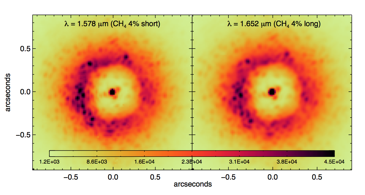
Figure 1: NICI Campaign images of the star HD 27290 seen through the focal plane mask, simultaneously obtained in the methane filters. The red channel image (right) has been rotated to match the sky PA of the blue channel image. The speckle pattern in the red channel is very similar to that in the blue channel but is larger in angular scale by roughly 4.6% (the ratio of the central wavelengths of the two filters). The halo in the red channel is also $\sim$5% fainter, because of slightly better halo suppression at that wavelength. The intensity scale is linear between -9$\times 10^{3}$ and 4.5$\times 10^{4}$ counts beyond which the scale ends. The counts in the blue channel image at the stellar peak is 1.1$\times 10^{5}$.

Our observing modes have been described in detail in Wahhaj et al. (2011). To summarize, we use two modes, ADI (Angular Difference Imaging) and ASDI (Angular and Spectral Difference Imaging), for each target in order to optimize sensitivity to both methane-bearing and non-methane bearing companions. In the ASDI mode, we observe simultaneously in two medium-band ($\Delta\lambda/\lambda=$4%) methane filters, $CH_{4}$S ($\lambda=$1.578 $\mu$m) and $CH_{4}$L ($\lambda$=1.652 $\mu$m), using NICI’s dual camera (Figure 1). In ADI mode, we only image in the $H$-band. In both observing modes, the primary star is placed behind a partially transmissive ($\Delta CH_{4}$S = 6.39 mag) coronagraphic mask with a half-power radius of 0.32^′′.

2.1 The ADI mode

When using the ADI technique, the telescope rotator is turned off, and the FOV rotates with respect to the instrument detectors. This is done so that the instrument and the telescope optics stay aligned with each other and fixed with respect to the detector. The respective speckle patterns caused by imperfections in the telescope and instrument optics are thus decoupled from any astronomical companions. In the de-rotated stack of images, the sky rotations of individual images are aligned. Thus, the speckle pattern is therefore azimuthally averaged, allowing the signal-to-noise of any point source in the field to improve as the square-root of integration time. This rate of improvement will only be achieved if the rotational offset between adjacent images is greater than the FWHM (Full Width at Half Maximum) of the PSF. Otherwise, the speckle-dominated regions in neighbouring images in the stack will be correlated and to some extent, the speckles will add as if they were signal. Finally, a reference PSF made by stacking the speckle-aligned images is subtracted from the individual images, so that some fraction of the speckle pattern is removed before it is azimuthally averaged. Thus the noise in the final stacked image is further reduced.

At large separations from the target star ($\gtrsim$ 1.5″), our sensitivity is limited by throughput, not by residual speckle structure. Thus the benefit of the ADI-only mode is that all the light is sent to one camera, to achieve maximum sensitivity. In this observing mode, we choose to acquire 20 1-minute images using the standard $H$-band filter, which is about four times wider than the 4% methane filters.

2.2 The ASDI mode

To search for close-in planets, we combine NICI’s angular and spectral difference imaging modes into a single unified sequence that we call “ASDI”. In this observing mode, a 50-50 beam splitter in NICI divides the incoming light between the $CH_{4}$S and $CH_{4}$L filters which pass the light into the two imaging cameras, henceforth designated the “blue” and “red” channels respectively. The two cameras are read out simultaneously for each exposure and thus the corresponding images have nearly identical speckle patterns. In effect, we have captured the rapidly changing atmospheric component of the speckles. However, because of differences in the light path of the two cameras and the wavelength-dependence of the speckles, the red channel PSF is not a perfect match to the blue channel PSF. The long-lived components of the speckle patterns in both channels are better captured in the remaining images of the full ASDI sequence, from which we can construct a reference PSF for further subtraction. In the ASDI Campaign mode, we typically choose to acquire 45 1-minute frames.

2.3 Observing constraints

Exposure times per frame are kept around 1 minute so that the time spent on detector readouts during an observing sequence is small. The hour angles when we observe our targets are chosen such that the rotation rate of the sky is less than 1 degree per minute to avoid excessive smearing during an individual exposure. The total sky rotation over the observing sequence is also required to be greater than 15 degrees, to minimize self-subtraction of companions at small separations (Biller et al., 2009).

For most targets, the exposure time per coadd in the ASDI mode is set small enough so that the star’s image behind the focal plane mask does not saturate. However, if this time is too small ($\leq$4 secs), a striping pattern resulting from electronic interference between the detectors during readout become prominent in the images. Thus for stars with $H<4$ mag, the star behind the mask and some part of its halo are allowed to saturate. For these data sets, we obtain short-exposure (unsaturated) images of the star behind the mask before and after the regular sequence. For faint stars, in individual images of 1-minute integrations, the final noise contribution from the speckles is smaller than the photon noise in the halo. So the ASDI mode ceases to yield an advantage. Thus, For stars with $H>7$ mag, we observe only in the ADI mode, but obtain 45 images instead of the usual 20.

3 DATA REDUCTION

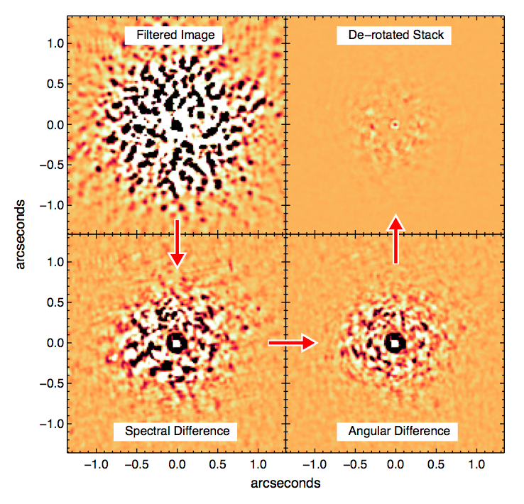
Figure 2: Partially reduced images after steps 2 through 6 of the NICI pipeline as described in the text. These images are from the reduction of the NICI observation of the star, HD 27290. The faint square pattern, somewhat discernible in the bottom two panels, is due to a striping pattern in the images. The total integration time for this ASDI observation was 45 minutes.

In our standard ASDI reduction, we reduce the images in six steps (see Figure 2):

1. Do basic reduction: apply flatfield, distortion and image orientation corrections.

2. Determine the centroid of the primary star.

3. Apply image filters (e.g. smoothing).

4. Subtract the red channel from the blue channel (SDI).

5. Subtract the median of all the images from the individual difference images (ADI).

6. De-rotate each individual image to a common sky orientation and then stack the images.

Step 1: Basic reduction Flatfield images were obtained during most NICI Campaign observing runs, and thus most datasets have corresponding flatfields obtained within a few days of their observing date. The images are divided by the flatfield. We estimate pixel-scale uncertainties of 0.1%, the fractional difference between two halves of a set of flatfield images. Bad pixels and cosmic ray hits are replaced by the median of the nearest eight good pixels. The distortion corrections used for the NICI data sets are available on the Gemini South NICI website. The correction is calculated from images of a rectangular focal-plane grid mask, upstream of the AO system, which captures the distortion introduced by both the AO system and the camera optics. To estimate the contribution of image distortion to astrometry, we compared two epochs of Proxima Centauri observations. There were 73 stars in these NICI images. We estimated the astrometric uncertainties to be 4 mas and 6 mas at separations of 3^′′ and 6^′′ from the center of the detector, respectively (see § 7.3). This distortion correction is an improvement over that used in Wahhaj et al. (2011).

When using ADI, the position angle (PA) of North in the individual NICI images are recorded in the FITS image headers at the beginning of the integrations. However, since the instrument rotator is turned off, over the course of an individual integration (1 min), the PA changes. We compute the PA value corresponding to the middle of the integration and add it to the FITS headers. This corrected PA is used later when de-rotating the individual images to a common orientation.

Steps 2 & 3: Centroiding and filtering In NICI Campaign datasets, the primary star is usually unsaturated as it is imaged a through a coronagraphic mask which is highly attenuating ($\Delta CH_{4}$S = 6.39$\pm$0.03 mag, $\Delta H=$5.94$\pm$0.05 mag; Wahhaj et al., 2011). Thus the location of the primary star in these images is easily determined and then recorded in the FITS headers, to be used later for image registration. The centroiding accuracy for unsaturated peaks or peaks in the non-linear regime is 0.2 mas (see §7.3). In ASDI datasets for bright stars (H $<$ 3.5 mag) and in most ADI datasets, the primary is saturated. In these images, the peak of the primary is still discernible as a negative image. We have estimated that the centroiding accuracy of the saturated images is 9 mas by comparing these to the centroids of unsaturated short-exposure images obtained right before and after the long exposures. For reference, the diffraction-limited FWHM in $H$-band is 43 mas and the NICI blue-channel plate scale is 17.96 mas.

Each red and blue channel image in a NICI dataset is processed by a software filter to isolate the contribution from point sources (quasi-static speckles and real objects) from the more diffuse light of the stellar halo. We describe how we chose the best filter in §4. In the end, we use the following procedure: (1) convolve the image with a Gaussian of 8 pixel FWHM, (2) subtract the convolved image from the original image to remove the diffuse PSF light and (3) convolve the resulting difference image with a Gaussian of 2 pixel FWHM to suppress the noise on the scale of individual pixels. This approach is quite effective at isolating the flux from point sources which have typical FWHM of 3 pixels.

Step 4: SDI subtraction We shift, rotate and demagnify the red channel images to match the speckles on the corresponding blue channel images. The speckles are matched over a 10 pixel wide annulus centered on the primary, with inner and outer radii of 0.65^′′ and 0.83^′′, respectively. This region is outside the coronagraphic mask, which is completely transparent at separations greater than 0.55^′′. Five parameters are optimized to find the best match between the two images: (1) shift in the horizontal direction; (2) shift in the vertical direction; (3) angular rotation offset; (4) radial demagnification; (5) intensity scaling. The match is determined by minimizing the RMS of the pixel values in the annular region in the difference image, using a simplex downhill routine (IDL routine AMOEBA; also see Press, W. H., Teukolsky, S. A., Vetterling, W. T., & Flannery, B. P., 1992). We use cubic interpolation to estimate the pixel values when rotating and shifting images. The relative rotation between the two channels is now known to a precision of 0.1^∘, based on imaging of dense fields. However, to be cautious, we still fit for the best angular offset between the two channels. For reference, the fractional increase in the RMS of the residual image is 1%, 5% and 100% for angular offset errors of 0.1^∘, 0.2^∘ and 1^∘, respectively.

Step 5: ADI subtraction Using the pre-computed centroids, all the difference images are registered. Then a reference PSF image is created by taking a median combination of the registered images. The motion of the star relative to the coronagraphic mask over course of the observation can cause shifts in the speckle pattern. Thus, the reference image is matched and subtracted from the individual difference images, optimizing the translational shift and intensity scaling. We caution here that a reference PSF subtraction may not only reduce the background RMS, but also remove some of the signal of a real object. However, such signal loss is significant only when the total sky rotation in an observation sequence results in an offset less than about twice the FWHM of the PSF at the angular separation of the object.

Step 6: De-rotation and stacking The double-differenced images (post-SDI and ADI subtraction) are now registered using the pre-computed centroids. At this step we are interested in aligning astronomical objects, not speckles. Also, using the previously computed PAs of the sky orientation, the images are de-rotated to orient North up. We compute the median of the stack of images to produce the final reduced image. At the edges of the field, only a subset of images contribute to the final image, since the square images have different sky orientations and thus non-overlapping regions.

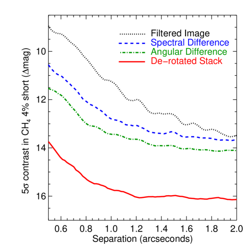
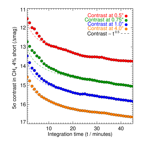
Figure 3: Left: Contrast curves (5$\sigma$) after step 2 through 6 of the NICI pipeline as described in the text. The curves computed after steps 3–5 are for an individual image, while the curve computed after step 6 represents the contrast limit on the stack of images. These contrast curves are from the reduction of the NICI images of the star HD 27290. The total integration time of this ASDI observation was 45 minutes. Right: Contrast versus integration time at different projected separations from HD 27290. The contrast improves roughly as $\sqrt{time}$.

The contrast achieved after each of the reduction steps for the NICI observation of HD 27290 is shown in the left panel of Figure 3. The fact that the improvement in contrast from stacking the difference images is roughly equal to the square root of the number of images in the stack implies that the residuals in the images are not correlated. That there is more than 2$\times$FWHM of rotational offset between frames at relevant angular separations is all that is necessary for this rate of contrast gain. As we see in the right panel of Figure 3, the contrast improves slightly faster than the square root of the integration time. This is probably because the Strehl ratio improved over the course of the observation. The ADI reduction is the same as the ASDI reduction, except that with ADI we are only dealing with one channel and so we do not perform the SDI reduction in step 4.

4 MEASUREMENT OF ACHIEVED CONTRAST VIA SIMULATED COMPANION RECOVERY

In this section, we describe a method to measure the contrast limit of NICI Campaign observations using simulated companions. We use scaled versions of the primary as seen through the focal plane mask to create these simulated companions. We have two goals for such work. The first goal is to measure the contrast at which 95% of the companions are recovered by different reduction pipelines (see § 5 & 6), and thereby identify the superior pipelines. We chose the 95% limit because, as will be clear later, an estimate of the 99% completeness limit takes roughly 5 times longer to compute. The second goal is to estimate the systematic and random errors introduced into the photometric and astrometric properties of the images by the reduction process. The method to do this is conceptually described below and then in greater detail in subsequent subsections.

Our method is to reprocess each data set with two modified reductions. The first reduction is to purposefully mis-rotate the frames so that the result does not contain any companions (a source-free reduction). This allows us to (1) set an upper contrast limit above which no detections (false positives) will be accepted and (2) determine the nominal 1$\sigma$ detection-limit curve. For the second reduction, we introduce fake companions 20 times brighter than the previously determined 1$\sigma$ limit (the 20$\sigma$ limit). The photometric and astrometric properties of the recovered companions of known contrast from the second reduction provide an estimate for the systematic and random errors introduced by the pipeline. Finally, the recovered companions are reinserted into the source-free reduction at several locations, and scaled up in intensity (starting from zero flux) until they meet our detection criteria. The contrast (1$\sigma$ limit times the scale factor) at which 95% of the simulated companions are detected (95% completeness) establishes our contrast curve for that star.

4.1 Making a source-free image to determine the false-positive threshold

To remove any real objects in a dataset from the final reduced image, in step 6 of the reduction procedure, we artificially set the orientation of the images to thirty times their actual sky PA values. Since the the directions of North on the images are now incorrect, when the stack of images is oriented to a common PA and median-combined any real objects disappear. Moreover, we can now assume that any point-source detection in this reduction is a false positive and that valid detections must be at a higher sigma level than the strongest false-positive. This is the first criteria that a companion detection must satisfy (in the properly oriented and stacked images) to be considered real by our algorithm.

4.2 1$\sigma$ contrast curve measurement

Since the focal plane mask attenuation is measured using a photometry aperture of 3 pixel radius (Wahhaj et al., 2011), the contrast curve is also measured using apertures of the same radius. We create an image from the final source-free reduced image, replacing each pixel value by the aperture (radius = 3 pixels) flux centered on that pixel. We then calculate the noise as a function of radius in this aperture flux map from the standard deviation of all pixel values in an annulus. Thus, the 1$\sigma$ contrast curve is the product of: (1) the inverse of the noise curve, (2) the flux of the primary (seen through the mask) and (3) the mask attenuation.

4.3 Detection criteria

To extract sources from the reduced image, we create a signal-to-noise map. To do this, we divide each pixel in the reduced image by the standard deviation of all the pixel values in a narrow annulus containing the chosen pixel. Since there are no real sources in the signal-to-noise map of the source-free image, the counts in the brightest spurious detection set the threshold for believable detections. To detect the spurious point sources, we first convolve the signal-to-noise map by the star spot (a circular region of radius 5 pixels centered on the star). This is done so that realistically shaped point sources, as opposed to single bright pixels or an accidental cluster of bright pixels, are preferentially amplified in the signal-to-noise map. As an initial sample of possible detections, we then take all the pixels brighter than three times the pixel-to-pixel standard deviation of the convolved signal-to-noise image. Next, we shift the star spot to the same center as each of the putative detections and scale its flux to match the peak pixel values in the unconvolved map. We then calculate a detection-strength metric given by $flux/\chi_{\nu}^{2}$, where $flux$ is the aperture (3 pixel radius) “flux” of the putative detection in the unconvolved S/N map, and $\chi_{\nu}^{2}$ is the reduced $\chi^{2}$ from the comparison between the detection and the star spot within the aperture. The flux is included in this metric to distinguish strong detections from faint point sources at the 1$\sigma$ level which can also have $\chi_{\nu}^{2}$ close to unity. The error in the pixel values is assumed to be one, since this is a signal-to-noise map. We find that point sources with a detection-strength of $\geq$0.25 look credible to the eye. This is satisfactory because Gaussian PSFs with peak intensity 5 times greater than the RMS of a Gaussian background also give a detection strength of 0.25. Finally, for a detection to be considered real, it must satisfy both this detection-strength criteria and be above the no-false-positive threshold.

4.4 Insertion of simulated 20$\sigma$ companions

We insert simulated companions at the 20$\sigma$ level to estimate the random and systematic effects of the pipeline and also to measure recovery completeness. After basic reduction of the individual images (step 1 of the pipeline), we embed 20$\sigma$ simulated companions into the individual blue channel images, using our 1$\sigma$ contrast curve as reference. The simulated companions are assumed to be methane-rich, such that they have negligible flux in the red channel. Note that our final contrast curves will be adjusted later to account for the methane channel brightnesses for companions as a function of spectral types (§7.2).

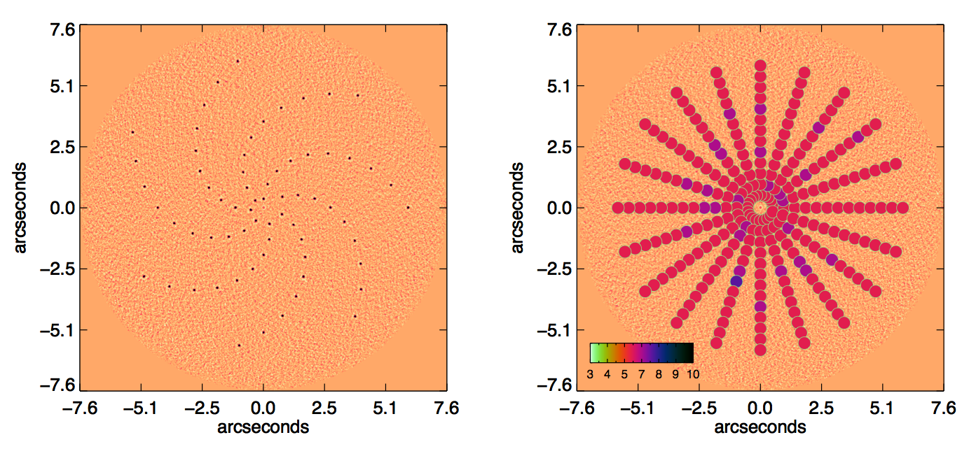
Figure 4: Left: Signal-to-noise map showing the recovery of simulated companions 20 times brighter than the 1$\sigma$ contrast curve. Right: Every 5^th ring of the 67 separation rings and 20 PAs at which the simulated companions were reinserted and recovered are shown with colored circles. The colors indicate the smallest signal-to-noise at which the companions satisfied the detection criteria. The color bar indicates the signal-to-noise scale. The image shown is the signal-to-noise map of the source-free reduction made from UY Pic data set of UT Dec 4, 2009.

The assumed sky PAs for the red and blue channel images are set to the same artificial values as in the source-free reduction, so that this final reduced image will be same, except for the embedded companions. The 20$\sigma$ companions are placed in each image at separations of 0.36^′′ to 6.3^′′ (20 to 350 pixels), with the first companion at 0.36^′′ separation and zero PA. Each subsequent companion is placed farther out by 0.09^′′ (5 pixels) and at a PA increased by 50 degrees (Figure 4). After the standard ASDI or ADI reduction procedure is applied and the signal-to-noise map is constructed, we easily recover all the simulated companions as roughly 20$\sigma$ detections. However, all the companions are recovered at different slightly contrasts than their original values and possibly have different fluxes depending upon the local effects of the reduction process. Our approach of generating the contrast (described below) naturally incorporates these effects.

4.5 Derivation of the 95% completeness contrast

The 20$\sigma$ companions in the signal-to-noise map at each separation (67 in total) are then cut out and inserted into the signal-to-noise map of the source-free reduction at 20 different PAs. At each location, we decrease the flux of the companion until it fails to satisfy our detection criteria. Remember that the two criteria are: (1) the source is above the false-positive threshold determined from the S/N map of the source-free image and (2) the source has good detection-strength which depends upon its total “flux” in the S/N map and PSF shape. Using these test insertions at each location, we record the maximum contrast (smallest companion flux) which resulted in detection. Thus, we know the contrast limit for each location. For each separation, we determine the contrast at which 19 out of 20 (95%) companions are recovered. The resulting curve represents the 95% completeness contrast. The right panel of Figure 4 shows the locations at which the recovered 20$\sigma$ companions were reinserted, i.e., where the contrast limits were determined. The standard contrast curve throws away information about the azimuthal variation of the contrast achieved. Figure 4 shows how much azimuthal variation there is in a typical reduction. The images shown are from the UY Pic ASDI data set obtained on 2009 December 4 UT.

5 OPTIMIZING IMAGE FILTERING VIA SIMULATED COMPANION RECOVERY

5.1 Description of the image filters

A better reduction should yield a better 95% completeness curve. Thus we use the 95% completeness curves to judge the effectiveness of different image filters in step 2 of the standard reduction procedure. The image filters we applied were different combinations of the following basic processes: “u’ unsharp-masking; “c” ’catch’ filtering (unsharp masking + smoothing); “a” removal of azimuthal profile and “d” de-striping. Unsharp masking is done by convolving an image with a Gaussian of 8-pixel FWHM and subtracting this convolved image from the original. Catch filtering entails a further smoothing with a Gaussian of 2-pixel FWHM in order to suppress pixel-to-pixel noise. The 2- and 8-pixel spatial scales are half and double the size, respectively, of the FWHM of the PSF in the poorer half of our data sets. The goal is to isolate to point sources. Azimuthal profiles were removed by a procedure described in Wahhaj et al. (2011). The procedure is very effective at removing PSF features which are extended azimuthally. De-striping is used to remove the striping pattern caused by detector electronics which usually occurs in short exposures. It is only applied to the region where the flux from the primary is fainter than twice the local pixel-to-pixel RMS. In this exterior region of the images, we subtract from each pixel the median of the closest 30 closest pixels in the same row, and then in the same column.

5.2 Comparison of the image filters

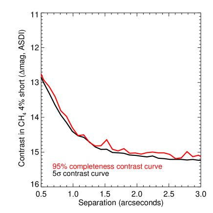
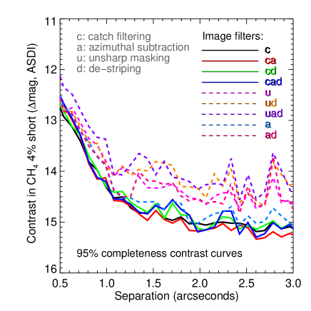
Figure 5: Left: The 95% completeness contrast curve (red line) compared to the 5$\sigma$ contrast curve (black line) as computed for the UY Pic 2009 Dec 4 data set. Right: The 95% completeness contrast curve for the same data set for several different image filters tested in the NICI pipeline. The different image filters are described in §5.1

Figure 5 shows the 95% completeness contrasts for different combinations of image filters used in the reduction of our UY Pic 2009 dataset. The filter ’cd’ indicates catch filtering followed by de-striping. We can see that the ’c’ filter yields the highest contrast close to the star, while at larger separations it yields one of the highest contrasts and also yields a smoother curve. The roughness of the other curves suggests that the other filters may be responsible for residual structures which are resulting in a patchy noise floor. The filter combinations that involve catch filtering yield better contrasts even at large separations where striping or sky noise dominates. It seems likely that the small-scale smoothing involved in catch filtering mitigates the problem of residual structures forming more complex patterns in the de-rotated reduced stack. At smaller separations, catch filtering leads to better fitting of the speckle pattern during the subtraction process. As expected, we found that the de-striping filter is more useful for datasets where the integration time per coadd is short, because the striping is more severe in these cases. We also make the following observations: (1) the best filters are ’c’, ’ca’, ’cd’ and ’cad’, and they are more or less equivalent; (2) the ’a’ and the ’d’ filters can slightly worsen performance when used together and (3) the catch filter generally improves performance. We choose the ’cad’ filter for the pipeline, as insurance against cases where the striping pattern or azimuthal variation across images is unusually severe. In Figure 5, we see that the 95% completeness curve agrees well with the nominal 5$\sigma$ noise curve for the UY Pic dataset.

6 COMPARISON WITH THE LOCI ALGORITHM

Algorithms for processing high contrast imaging have steadily improved at removing starlight while preserving the planet’s flux. Currently, the LOCI (Locally Optimized Combination of Images) algorithm is among the most commonly used post-processing method (Lafrenière et al., 2007a). It was originally used to process ADI data from the Gemini Deep Planet Survey (Lafrenière et al., 2007b). LOCI builds the optimal PSF for any given sub-region of the science image, choosing linear combinations of science images where the PSF is very similar. This algorithm has undergone several improvements. For example, the subtraction region can be masked so as not to bias the construction of a reference PSF by real companions (Marois et al., 2010a). Moreover, the subtraction region can reduced to one pixel, and LOCI choices tuned to improve point-source sensitivity (Soummer et al., 2011). Lastly, LOCI can be applied to integral field spectroscopy observations, where the reference PSF can be built from images of the star over an entire spectral and temporal range (e.g., Barman et al., 2011). Pueyo et al. (2012) have added the innovation that LOCI is programmed not just to minimize the local noise in the images but also to preserve the local flux. In other words, the algorithm tries to maximize the local signal-to-noise.

We can now compare the effectiveness of the original LOCI algorithm to that of our standard NICI Campaign pipeline using their respective 95% completeness contrast curves. The more sophisticated versions of LOCI (Soummer et al., 2011; Pueyo et al., 2012) designed for improved flux conservation are quite computationally intensive, and we do not test with them in this paper.

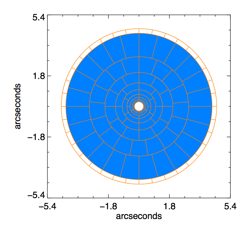
Figure 6: The subtraction and reference sectors for an example set of parameters in the LOCI algorithm, with $dr$ increasing at a rate of 50% ($dr_{fac}$=1.5) and number of sectors linearly increasing with radius, from 3 to 18. The reference regions extend beyond the subtraction regions radially by 15 pixels ($dw=$15). This extension is shown without color for the outermost ring.

The LOCI algorithm is applied in step 5 of our pipeline, after we subtract the red channel images from the blue channel images. In short, the algorithm works likes this. When processing each science image, instead of subtracting the median combination of the other images in the dataset, we subtract a linear combination of the images optimized for each region of the image. These regions are configured as segmented concentric annuli around the primary star (Figure 6). For each region that we want to optimally subtract speckles from, we define a reference region which extends outward radially from the subtraction region by an extra 15–30 pixels. The linear combination of images is optimized over the larger reference region to minimize the RMS of the subtraction.

The LOCI algorithm can be tuned by the following parameters: $N_{\delta}$, $N_{A}$, $dr$, $g$ and $dw$. $N_{\delta}$ represents the minimum offset required when selecting reference frames, measured as arclength traced by the sky rotation divided by the PSF FWHM. $N_{A}$ is the area of the reference region in units of the PSF FWHM, and $dr$ is the radial width of the subtraction region in units of PSF FWHM. The parameter, $g$, is the ratio of the radial extent to the angular extent of the reference region, and $dw$ is the extra radial width of the reference region beyond that of the subtraction region. For our LOCI processing, we assume a PSF FWHM of 3 pixels, which is representative of our NICI data.

Instead of setting $N_{A}$ and $g$ directly, we set it through two alternate parameters which are easier to conceptualize. We set the number of sectors in the annulus at $r=7^{\prime\prime}$ using by the parameter, $N_{sec}$. We choose the number of sectors per annulus to decrease linearly with decreasing radius, rounding the number to nearest integer. We increase the radial width of the subtraction regions geometrically going outwards by the factor $dr_{fac}$ with each annular increment. The $N_{A}$ and $g$ values corresponding to some of the $N_{sec}$ and $dr_{fac}$ values we used are given in Table 1. Our choice of sectors for an example set of LOCI parameters is shown in Figure 6.

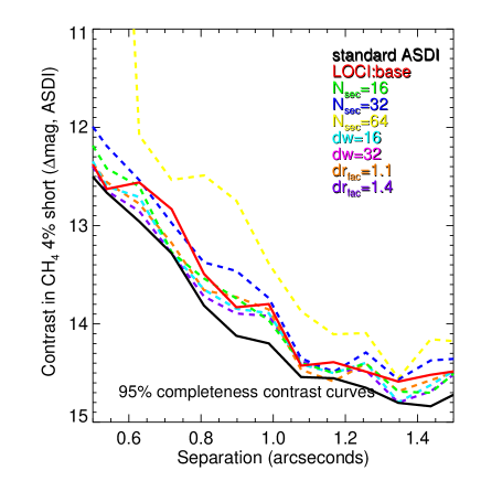
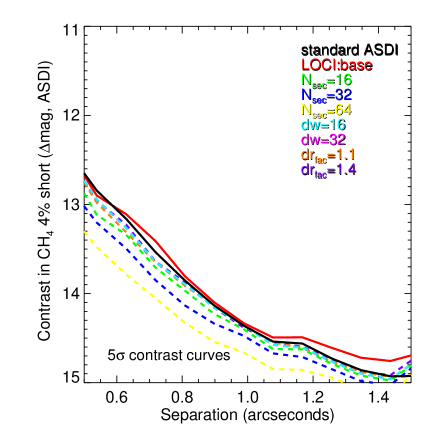
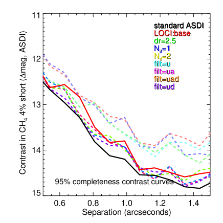
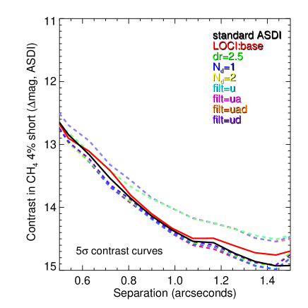
Figure 7: Left (top and bottom): Comparison of 95% completeness contrasts for different LOCI reductions and our standard ASDI reduction for UY Pic two-channel ASDI 2009 data. The LOCI base parameters were set to $N_{sec}=8$, $N_{\delta}=3$, $dr=4$, $dr_{fac}=1.2$, $dw=1$ and filt = ’cad’ (see text for explanation). For the other LOCI reductions, we set only one parameter to a different value as noted in the legends. Also shown is the 95% completeness contrast (black line) for the standard ASDI algorithm. The LOCI reductions are not an improvement on our standard ASDI reduction. Right (top and bottom): Comparison of the nominal 5$\sigma$ contrast curves.

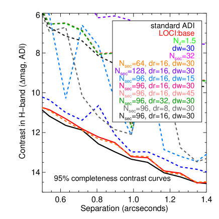
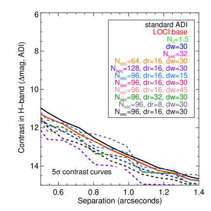
Figure 8: Left: Comparison of 95% completeness contrasts for different LOCI reductions and the standard reduction for UY Pic one-channel ADI 2009 data. The LOCI base parameters were set to $N_{sec}=8$, $N_{\delta}=3$, $dr=4$, $dr_{fac}=1.2$, $dw=1$ and filt = ’c’ (see text for explanation). For the other LOCI reductions, we set some parameters to different values as noted in the legends. Also shown is the 95% completeness contrast (black line) for the standard ADI algorithm. The LOCI reductions do not show any improvement over the standard ADI reduction. Right: Comparison of the nominal 5$\sigma$ contrast curves.

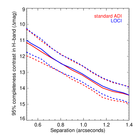
Figure 11: Comparison of median contrast curves from the NICI standard ADI reduction (red) and the best LOCI reduction (blue) for 45 NICI ADSI data sets obtained in 2009. The median completeness curves are drawn as solid lines, while the 1$\sigma$ range is shown by the dashed lines.

We tested the performance of several sets of parameters in the LOCI algorithm for our December 2009 UY Pic ASDI data set (45 images, each of 60 sec exposure time; total sky rotation of 34^∘). All combinations of parameters for $N_{sec}=\{8,16,32\}$, $dw=\{16,32\}$, $dr=\{2,4,6\}$ and $N{{}_{\delta}}=\{0.5,1\}$ were evaluated. However, no LOCI reduction yielded a noticeable improvement over the standard ASDI reduction, when comparing the 95% completeness curves. At the same time, we found that the LOCI reductions can produce final images with less noise. In the left panel of Figure 7, we demonstrate the effect of changing each LOCI parameter from a base set of values. Although none of the LOCI 95% completeness curves improve on the standard ASDI curve, in the right panel of Figure 7 we see that the LOCI reductions yield better nominal 5$\sigma$ contrast curves. In the fact, the more aggressive LOCI reductions (smaller subtraction regions, etc.) yielded better nominal 5$\sigma$ contrast curves but worse 95% completeness curves. Even for the plain one-channel ADI UY Pic data set, the LOCI 95% completeness curves showed no improvements over the standard reduction (Figure 8). This result was confirmed when we took 45 ADI Campaign datasets from 2009 (see §7) and compared their 95% completeness contrasts from LOCI and our standard ADI pipeline (Figure 11).

Our results differ from those of Lafrenière et al. (2007a) perhaps because we use a detection criteria to define our completeness curve, rather than just the radial noise profile. In their work, Lafrenière et al. (2007a) compare the signal-to-noise of recovered simulated companions for LOCI and non-LOCI algorithms but do not set a criteria for what counts as a detection, or consider the false-positive threshold. Another possible explanation for the different results is that the higher Strehl ratios achieved with NICI (Chun et al. 2008) have yielded more stable quasi-static speckle patterns than obtained with the Gemini/ALTAIR AO system for GDPS. In this case, the special selection of reference frames with LOCI would not be very effective, because the reference frames are all comparably good matches. Experimentation with NICI data sets longer than the Campaign stardard of 45 mins, where the quasi-static pattern changes significantly over the course of the observation, might show that in these cases, LOCI performs better. However, that experiment is beyond the scope of this paper.

Lafrenière et al. (2007a) have already explained that LOCI can remove signal from real objects in the field if applied too aggressively. When the reference regions are too small or the reference images too numerous, the application of LOCI is too aggressive. In practice, even when reference images are bad matches to the science image, as the number of images is increased, LOCI keeps reducing the noise in the output image. Thus it is advisable to check that simulated companions that are brighter than the contrast limits are not lost in the reduction process. Using the same method, one can also check that the contrast of the simulated companions are correctly recovered (Marois et al., 2010a).

7 ANALYSIS OF NICI CAMPAIGN DATA FROM 2009A

Since the NICI Campaign began in December 2008, we have obtained 172 ASDI data sets and 241 ADI data sets as of August 2012. Since performing the simulated companion tests on all the Campaign data is time-consuming, we limit our analysis to 45 ASDI and 45 ADI data sets obtained in the beginning of 2009. Some NICI targets have either only an ASDI or only an ADI observation, and so some of the targets in our ASDI and ADI sample data sets are different. We chose the standard ASDI reduction method over LOCI, since we noticed no improvement with the latter method (§6). Figure 11 also shows that the NICI standard ADI pipeline and the LOCI pipeline gives the same performance for the 2009 ADI data sets. As before, we generate the 95% completeness contrasts for all our data sets.

7.1 Achieved raw contrasts

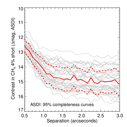
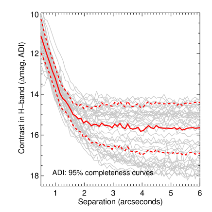
Figure 9: Left: 95% completeness contrasts from 45 NICI ADSI data sets obtained in 2009. Completeness contrasts from individual data sets are shown in gray. The median completeness curve is drawn as a solid red line, while the 1$\sigma$ range is shown by the dashed red lines. Right: 95% completeness contrasts from 45 NICI ADI data sets obtained in 2009. Some of the stars in the ASDI and ADI samples are different.

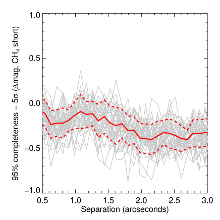
Figure 10: The difference between the 95% completeness and the 5$\sigma$ constrast curves for 45 NICI ADSI data sets obtained in 2009. The contrast differences from individual data sets are shown in gray. The median difference curve is drawn as a solid red line, while the 1$\sigma$ range is shown by the dashed red lines.

Figure 9 shows all the individual ASDI and ADI 95% completeness curves and also the median curve and the 1$\sigma$ dispersion. For this set of stars ($V=$ 4.3–13.9 mag), we should have recovered 95% of companions with a median ASDI contrast less than 12.6 mags at 0.5^′′ and less than 14.4 mags at 1.0^′′. The difference between the 95% completeness curves and the nominal 5$\sigma$ curve for each dataset is displayed in Figure 10 for comparison. The median 95% curve is poorer than the median 5$\sigma$ curve by 0.1 and 0.3 mag at 0.5^′′ and 3^′′, respectively, varying slowly with separation. The difference is smallest at separations dominated by the stellar halo, increases with separation, and is roughly flat at separations beyond 2^′′.

At low temperatures ($<$1400 K), substellar objects with spectral type T (Baraffe et al., 2003), exhibit methane absorption in their spectra, such that their red channel flux would be suppressed relative to their blue channel flux. However, these considerations only become important when we are trying to calculate companion mass sensitivities. So, we defer such a discussion to §7.2.3. Here, we just note that even for an object with no methane, there is little self-subtraction from the red channel beyond separations of 1^′′, since we radially stretch the red channel image before SDI subtraction. Inside of 1^′′, for objects without any methane, the reduction of the ADI-mode dataset or the separate ADI reductions of the red and the blue channels should yield better sensitivities as the red channel flux is not subtracted in these.

Beyond a separation of 1.5^′′, the ADI $H$-band contrast curves are more sensitive, with 95% completeness contrasts of 15.0 and 15.5 mag at 1.5^′′ and 3^′′, respectively. Beyond 3^′′, the ADI median completeness curve flattens out, as the noise from the sky background and detector readout begin to dominate that from the halo. Note that at large separations the ADI contrast distribution in Figure 9 is bimodal. This is because for faint stars, we reach the background limit at smaller angular separations than for bright stars, and the brightness distribution of our primary stars is also roughly bimodal. The distribution of contrasts at large separations is also skewed such that the mean contrast (16.0 mag) is greater than the median contrast (15.5 mag).

7.2 Contrast curve adjustments

The simulated companions used to estimate the contrast curves are not subject to the same alterations to their flux that real objects in the field are. To adjust the contrast curves for these alterations, we take into account three effects: (1) smearing of an object’s flux as the field rotates during each individual exposure; (2) the non-zero mask opacity from 0^′′ to 0.55^′′ separation from the primary; and (3) the flux loss from the red and blue channel differencing for objects that do not have photospheric methane absorption.

Note that another important effect, the contrast alteration due to ADI self-subtraction, is already accounted for in the 95% completeness curves, since the simulated companions used to construct the curve undergo the same alteration as any real object.

7.2.1 Smearing correction

The representative area of a PSF core is $\pi a^{2}$, where $a$ is the half width at half maximum of the PSF, or about 1.5 NICI pixels. Due to sky rotation during an individual exposure, the flux in the PSF core is spread over an area $\pi a^{2}+2aL$ (Lafrenière et al., 2007b). Here, $L$ ($=R\omega\Delta t$) is the arclength traced by a real object during an individual exposure, $\Delta t$ ( typically 1 minute for NICI observation). The separation from the primary and the rotation rate in radians per minute are $R$ and $\omega$, respectively. Thus, there is a fractional flux loss of $1+(2R\omega\Delta t)/(\pi a)$ in the PSF core. We convert this loss into magnitudes as a function of separation and subtract it from the 95% completeness contrasts. Out of 413 NICI observations obtained up to August 2012, 382 (93%) of NICI observations have an average rotation rate of less than 2 degrees per minute. Thus, 93% of the time the contrast is degraded by less than 0.015 and 0.08 magnitudes at 1^′′ and 5^′′, respectively.

To check the reliability of the flux correction, we simulated the smearing of Gaussian PSFs (FWHM= 3 pixels) for the target declinations and observing hour angles that yield very fast and non-uniform rotation rates. We tested declinations from -24^∘ to -36^∘ (Gemini South latitude$=-$30.24^∘) in steps of 2^∘ and starting hour angles of $+$10 and $-$10 minutes. These choices yielded average rotation rates of 1 to 3.5^∘ per minute. We placed the PSF at a separation of 3^′′ from the rotation center. For larger separations, one can use the superior ADI detection limits obtained with small rotation rates and thus avoid the smearing problem. We then measured the 3-pixel (radius) aperture flux of the median-combined 45 frames of smeared PSFs from the varying sky rotations. This aperture flux was adjusted for the flux loss fraction we computed earlier and compared to the true aperture flux of the Gaussian PSF. We found in all cases that the fractional difference was less than 1.5%. This precision is high enough for our purposes.

7.2.2 Mask opacity correction

As described in Wahhaj et al. (2011), we observed a pair of stars, (2MASS J06180157–1412573 and 2MASS J06180179–1412599) separated by only a few arcseconds, to measure the opacity of the coronagraphic mask in the $CH_{4}$ 4% short and long filters. The two stars were observed simultaneously without the mask and then observed with the brighter object at different displacements along a straight line from the center of the mask. We measured the contrast between the stellar pair in the off-mask images and in the mask-occulted images, using an aperture radius of 3 pixels. The difference between the on and off-mask contrasts (in magnitudes) gives us the mask opacity between 0^′′ to 0.55^′′ from the center of the mask. The measured opacities of the 0.32^′′ (radius) mask as a function of separation are given in Table 2. At the center of the mask, the opacity is 6.39$\pm$0.03 mag, while at a separation of 0.55^′′ the mask becomes completely transparent. The uncertainty in the opacity is dominated by the uncertainty in the astrometry of a detected source through an opacity gradient. Our measurements have shown this astrometric uncertainty to be roughly 0.5 NICI pixels (9 mas). The opacity uncertainties given in Table 2 are the standard deviation of opacity values over 9 mas ranges.

For the $H$-band, used in the ADI observations, we only have measurements of the central mask opacity. Thus for targets where we only conducted ADI observations, the $CH_{4}$ mask opacity adjustment is used, assuming that the $H$-band transmission profile has the same shape. The final sensitivity limits for a target star only depend on the better of the ASDI and ADI contrasts achieved at each separation. At separations of less than 0.55^′′, the ASDI observations taken with $CH_{4}$ filters always yield superior contrasts, so our lack of independent data for the $H$-band does not impact our survey results.

7.2.3 SDI self-subtraction correction

In the ASDI reduction, when the red channel image is demagnified to matched the speckles in the blue channel image, at large enough separations ($>$1.2^′′) the red channel counterpart of a real object will almost completely shift off the blue channel counterpart. However, at small separations the red and blue channel counterparts will still overlap. Thus during image differencing, some flux from the blue channel will be removed and this has to be adjusted for. Of course, this SDI self-subtraction correction does not affect the ADI contrast curves. We do not apply this correction to the ASDI contrast curves for the Campaign. Instead, we apply the correction when converting the ASDI contrast curves into companion-mass sensitivity curves, for which we have to assume a spectral type (e.g., T dwarf). Monte Carlo simulations are used to determine the planet detection probability of each NICI observation (Nielsen et al., 2013). In these simulations thousands of companions of are drawn from a power-law distribution in mass. Using evolutionary models (e.g. Baraffe et al., 2003), the temperatures corresponding to the masses of the simulated companions are computed, given the age of the host star. Next, we calculate the red to blue channel flux ratio given the temperatures of the companions and assumed spectral type to temperature relation. Thus, we can estimate the ASDI contrasts of the companions and what fraction of them are expected to be detected given the measured contrast curve. In other words, the SDI correction is not applied to the contrast curves themselves but to the model-derived contrasts of simulated companions.

The fractional flux loss due to SDI subtraction is a function of separation. We estimate this loss by subtracting a Gaussian PSF of width 3 pixels from itself after shifting it radially by 4.6% of the separation (which corresponds to red image demagnification) and taking the ratio of its fluxes before and after the subtraction. This maximum fractional loss is for objects without methane absorption. For T dwarfs, the red channel has less flux than the blue channel due to methane absorption, and thus the loss is less severe for these objects.

Using the spectrum of 2MASS J04151954$-$093506 (spectral type T8 Knapp et al., 2004; Burgasser et al., 2006), we estimate that companions of spectral type T8 have a red to blue channel flux ratio of 0.125. Thus, during the ASDI reduction process, at small separations roughly 0.125 mag of flux may be removed when subtracting the red channel from the blue channel. To recover the true CH₄ 4% short (blue channel) sensitivity to a T8 at small separations, we need to decrease the contrast estimate from the ASDI reduction by 0.125 mags.

We find that even with significant self-subtraction, the ASDI reduction can yield superior contrasts to the ADI reductions. For example, for a companion with no methane, the ASDI contrasts at 0.5^′′, 0.75^′′ and 1.0^′′ separation are reduced by 0.58, 0.49 and 0.2 mags, respectively, relative to its blue channel contrasts. Comparing the median contrast curves in Figure 9, we note that the ASDI curve is more sensitive than the ADI curve by 1.5, 1.35 and 0.9 mags at the same separations, respectively. Thus at small separations, the ASDI contrast curves are typically more sensitive, whether the companions are methane-bearing or not.

7.3 Photometric accuracy

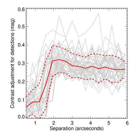
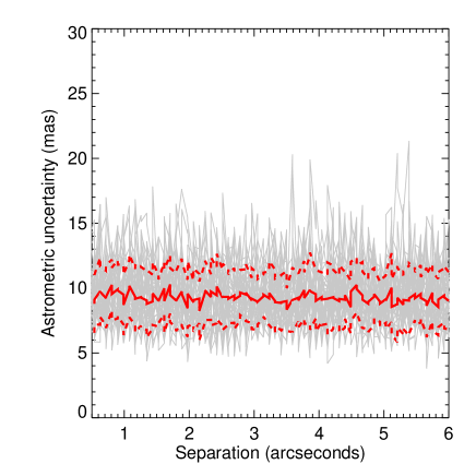
Figure 13: Left: Contrast adjustment to be applied to the photometry of detected companions. This adjustment or systematic error was estimated from 45 ASDI data sets from 2009. The adjustments for individual data sets are shown in gray. The median adjustment and the standard deviation are shown as a function of separation in red solid and dashed lines, respectively. Right: The astrometric uncertainties estimated from the same reductions. Individual, median and standard deviation curves are shown in the same color scheme as the left figure.

Our image reduction procedure introduces small systematic and random errors into the photometry of detected objects. Here, we estimate there errors by studying the recovered simulated companions. The original simulated companions were inserted into the individual frames as 20$\sigma$ sources relative to the $1\sigma$ contrast curve (§ 4.3). When these are recovered after the reduction procedure, their measured contrast with respect to the primary is differs from the original value. The differences between the input contrasts and the recovered contrasts for the 2009 ASDI data sets are plotted against separation in Figure 13. At each separation, we plot the median of the contrast difference as a solid line and indicate the standard deviation by two dashed lines. The contrast difference increases from 0.05 to 0.3 mags between 0.5 and 2^′′ and settles to 0.25 mags at 6^′′. The standard deviation suggests a uniform photometric uncertainty of 0.07 mags between 0.5 and 6^′′. We use these results to correct the photometry of detected companions. (Note that the 95% completeness curves do not require this correction.)

7.4 Astrometric accuracy

The reduction procedure also introduces some astrometric uncertainty in the location of companions with respect to the primary. We plot the astrometric displacement between the original locations of the artificial companions and their recovered locations in Figure 13. (The uncertainty is of course expected to be smaller for brighter companions.) We see that the astrometric uncertainty is roughly uniform ($\approx$ 10 mas) as a function of separation. However, we must also include the uncertainties introduced by centroiding, residual distortions and the plate scale estimate.

The astrometric uncertainty due to the precision limit of our centroiding algorithm, given the finite size of the NICI pixels, is 0.011 pixels (0.2 mas). We estimate this by testing our centroiding algorithm on Gaussian point sources placed in a noise-free image with different sub-pixel offsets relative to the pixel center. The standard deviation of the difference between the known positions and the measured positions of the point sources gives the uncertainty of the centroiding algorithm.

For saturated datasets, we compare the centroids of the short exposure unsaturated images, taken just prior to the science data, to the centroid estimate of the first saturated image. The movement of the star relative to the mask should be very small for the minute of elapsed time between the exposures. From analyzing several saturated datasets, we estimate that the centroiding uncertainty for saturated images is 0.5 pixels or 9 mas.

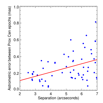
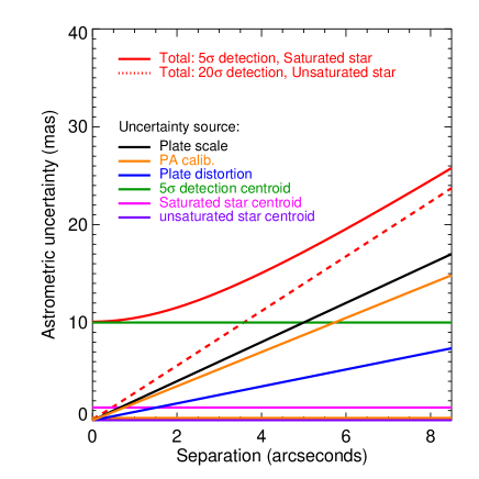
Figure 12: Left: Astrometric error between two epochs of Prox Cen NICI observations taken on UT 2009 April 8 and April 26. The 57 detections with signal-to-noise above 30 are shown. These were used to produce a robust line-fit for error vs separation (red line). Right: NICI astrometric errors from all the known sources as a function of separation (see text). The total errors for two cases are shown: (1) sources found at the detection limit in a dataset with a saturated primary, and (2) sources detected at the 20$\sigma$ level around an unsaturated star.

The astrometric uncertainty due to imperfect distortion correction was found to be 0.017+0.049$\rho$ pixels, where $\rho$ is the projected separation in arcseconds. This was measured by comparing the detections in the Proxima Centauri field from two NICI epochs obtained on 2009 April 8 and April 26 UT. Out of 73 background sources, the differences in the positions of 57 sources with S/N$>$30 were fitted robustly with a line (Figure 12), which resulted in the solution above.

The red and blue channel plate scales were measured from NICI observations of a field in the Large Megallanic Cloud. This field has been observed with Hubble Space Telescope Advanced Camera for Surveys to an astrometric precision of 1 mas (Diaz-Miller 2007). The astrometric uncertainty in the NICI plate scale measurement is estimated to be 0.2%. From these observations, we also estimated that the uncertainty in the direction of North is 0.1 degrees.

The total astrometric error is all these contributions added in quadrature. Figure 12 shows all the contributions as a function of separation. The total astrometric uncertainty for a 20$\sigma$ source detection around an unsaturated star is 2.2 and 11 mas at 1^′′ and 5^′′, respectively. The total astrometric uncertainty for a 5$\sigma$ source detection around a saturated star is 10 and 15 mas at 1^′′ and 5^′′, respectively.

8 CONCLUSIONS

We have presented the image processing techniques used to detect companions to target stars in the Gemini NICI Planet-Finding Campaign. We have achieved median contrasts of 12.6 magnitudes at 0.5^′′ and 14.4 magnitudes at 1^′′ separation, for a sample of 45 stars ($V=$ 4.3–13.9 mag) from the early part of our campaign. We have also implemented a novel technique to calculate completeness contrast curves, accounting for both completeness and false positives. We have demonstrated how this technique can be used to determine which image-processing pipelines are more successful at recovering faint simulated point sources. Specifically, we analyzed the effect of different image filters on the final contrast curves. We have compared our pipeline to the performance of the LOCI algorithm on NICI data, and found that LOCI is not more effective than our standard pipeline.

Our processing technique is conceptually similar to previous techniques, but differs in that we use special image filters and fit speckle patterns prior to reference PSF subtraction. The next-generation exoplanet finders, SPHERE (Beuzit et al., 2010) and the Gemini Planet Imager (Macintosh et al., 2008), will both be equipped with integral field spectrographs (also see Oppenheimer et al. (2013); Project 1640 and Guyon et al. (2011); SCExAO) and will thus require more complex algorithms to isolate the exoplanet signals (e.g. Pueyo et al., 2012). However, for the faintest planets, some version of the ASDI method discussed here will probably have to be used as the signal will be too weak to obtain resolved spectra. Thus, the techniques demonstrated here may be instrumental in addressing exoplanet detection challenges of the future.

Table 1: Relation between LOCI parameters

$N_{sec}$, $dr_{fac}$, $dw$	$N_{A}$, $g$ at $r=0.5^{\prime\prime}$	$N_{A}$, $g$ at $r=7^{\prime\prime}$
8, 1.2, 16	690, 0.1	3400, 0.3
8, 1.4, 16	570, 0.1	4200, 0.35
32, 1.2, 16	340, 0.2	960, 1.1
32, 1.4, 16	320, 0.2	1000, 1.5
8, 1.2, 1	160, 0.04	2700, 0.2
8, 1.4, 1	160, 0.04	3500, 0.3
32, 1.2, 1	80, 0.07	690, 1.0
32, 1.4, 1	70, 0.07	840, 1.3

Table 2: Measured opacities of the 0.32^′′ (radius) mask as a function of separation.

Separation (′′)	$\Delta CH_{4}$ short (mag)	uncertainty (mag)
0.0	6.39	0.03
0.2	4.5	0.22
0.3	2.1	0.09
0.4	0.73	0.02
0.55	0.0	-

References

- Baraffe et al. (2003) Baraffe, I., Chabrier, G., Barman, T. S., Allard, F., & Hauschildt, P. H. 2003, A&A, 402, 701
- Barman et al. (2011) Barman, T. S., Macintosh, B., Konopacky, Q. M., & Marois, C. 2011, ApJ, 733, 65
- Beuzit et al. (2010) Beuzit, J.-L., et al. 2010, in Astronomical Society of the Pacific Conference Series, Vol. 430, Pathways Towards Habitable Planets, ed. V. Coudé Du Foresto, D. M. Gelino, & I. Ribas, 231
- Biller et al. (2013) Biller, B., Liu, M. C., Wahhaj, Z., Nielsen, E. L., et al. 2013, ArXiv e-prints
- Biller et al. (2009) Biller, B., et al. 2009, in American Institute of Physics Conference Series, Vol. 1094, American Institute of Physics Conference Series, ed. E. Stempels, 425–428
- Biller et al. (2010) Biller, B. A., Liu, M. C., Wahhaj, Z., Nielsen, E. L., et al. 2010, ApJ, 720, 82
- Biller et al. (2007) Biller, B. A., et al. 2007, ApJS, 173, 143
- Borucki et al. (2010) Borucki, W. J., et al. 2010, Science, 327, 977
- Bowler et al. (2010) Bowler, B. P., Liu, M. C., Dupuy, T. J., & Cushing, M. C. 2010, ApJ, 723, 850
- Burgasser et al. (2006) Burgasser, A. J., Geballe, T. R., Leggett, S. K., Kirkpatrick, J. D., & Golimowski, D. A. 2006, ApJ, 637, 1067
- Burrows et al. (1997) Burrows, A., et al. 1997, ApJ, 491, 856
- Chun et al. (2008) Chun, M., et al. 2008, in Society of Photo-Optical Instrumentation Engineers (SPIE) Conference Series, Vol. 7015, Society of Photo-Optical Instrumentation Engineers (SPIE) Conference Series
- Cumming et al. (2008) Cumming, A., Butler, R. P., Marcy, G. W., Vogt, S. S., Wright, J. T., & Fischer, D. A. 2008, PASP, 120, 531
- Ftaclas et al. (2003) Ftaclas, C., Martín, E. L., & Toomey, D. 2003, in IAU Symposium, Vol. 211, Brown Dwarfs, ed. E. Martín, 521
- Gladysz & Christou (2009) Gladysz, S., & Christou, J. C. 2009, ApJ, 698, 28
- Gould et al. (2010) Gould, A., et al. 2010, ApJ, 720, 1073
- Guyon et al. (2011) Guyon, O., Martinache, F., Clergeon, C., Russell, R., Groff, T., & Garrel, V. 2011, in Society of Photo-Optical Instrumentation Engineers (SPIE) Conference Series, Vol. 8149, Society of Photo-Optical Instrumentation Engineers (SPIE) Conference Series
- Howard et al. (2010) Howard, A. W., et al. 2010, Science, 330, 653
- Janson et al. (2013) Janson, M., et al. 2013, ArXiv e-prints
- Kalas et al. (2013) Kalas, P., Graham, J. R., Fitzgerald, M. P., & Clampin, M. 2013, ApJ, 775, 56
- Kalas et al. (2008) Kalas, P., et al. 2008, Science, 322, 1345
- Knapp et al. (2004) Knapp, G. R., et al. 2004, AJ, 127, 3553
- Kuzuhara et al. (2013) Kuzuhara, M., et al. 2013, ApJ, 774, 11
- Lafrenière et al. (2008) Lafrenière, D., Jayawardhana, R., & van Kerkwijk, M. H. 2008, ApJ, 689, L153
- Lafreniere et al. (2010) Lafreniere, D., Jayawardhana, R., & van Kerkwijk, M. H. 2010, ApJ, 719, 497
- Lafrenière et al. (2007a) Lafrenière, D., Marois, C., Doyon, R., Nadeau, D., & Artigau, É. 2007a, ApJ, 660, 770
- Lafrenière et al. (2007b) Lafrenière, D., et al. 2007b, ApJ, 670, 1367
- Lagrange et al. (2009) Lagrange, A., et al. 2009, A&A, 493, L21
- Lagrange et al. (2010) Lagrange, A.-M., et al. 2010, Science, 329, 57
- Leconte et al. (2010) Leconte, J., et al. 2010, ApJ, 716, 1551
- Liu (2004) Liu, M. C. 2004, Science, 305, 1442
- Liu et al. (2010) Liu, M. C., et al. 2010, in Society of Photo-Optical Instrumentation Engineers (SPIE) Conference Series, Vol. 7736, Society of Photo-Optical Instrumentation Engineers (SPIE) Conference Series
- Macintosh et al. (2008) Macintosh, B. A., et al. 2008, in Society of Photo-Optical Instrumentation Engineers (SPIE) Conference Series, Vol. 7015, Society of Photo-Optical Instrumentation Engineers (SPIE) Conference Series
- Marcy et al. (2008) Marcy, G. W., et al. 2008, Physica Scripta Volume T, 130, 014001
- Marois et al. (2005) Marois, C., Doyon, R., Racine, R., Nadeau, D., Lafreniere, D., Vallee, P., Riopel, M., & Macintosh, B. 2005, JRASC, 99, 130
- Marois et al. (2008) Marois, C., Macintosh, B., Barman, T., Zuckerman, B., Song, I., Patience, J., Lafrenière, D., & Doyon, R. 2008, Science, 322, 1348
- Marois et al. (2010a) Marois, C., Macintosh, B., & Véran, J.-P. 2010a, in Society of Photo-Optical Instrumentation Engineers (SPIE) Conference Series, Vol. 7736, Society of Photo-Optical Instrumentation Engineers (SPIE) Conference Series
- Marois et al. (2010b) Marois, C., Zuckerman, B., Konopacky, Q. M., Macintosh, B., & Barman, T. 2010b, Nature, 468, 1080
- Meshkat et al. (2013) Meshkat, T., et al. 2013, ApJ, 775, L40
- Nielsen et al. (2013) Nielsen, E., et al. 2013, ApJ, 776, 4
- Nielsen & Close (2010) Nielsen, E. L., & Close, L. M. 2010, ApJ, 717, 878
- Nielsen et al. (2008) Nielsen, E. L., Close, L. M., Biller, B. A., Masciadri, E., & Lenzen, R. 2008, ApJ, 674, 466
- Nielsen et al. (2012) Nielsen, E. L., et al. 2012, ApJ, 750, 53
- Oppenheimer et al. (2013) Oppenheimer, B. R., et al. 2013, ApJ, 768, 24
- Press, W. H., Teukolsky, S. A., Vetterling, W. T., & Flannery, B. P. (1992) Press, W. H., Teukolsky, S. A., Vetterling, W. T., & Flannery, B. P., ed. 1992, Numerical recipes in C. The art of scientific computing
- Pueyo et al. (2012) Pueyo, L., et al. 2012, ApJS, 199, 6
- Racine et al. (1999) Racine, R., Walker, G. A. H., Nadeau, D., Doyon, R., & Marois, C. 1999, PASP, 111, 587
- Rameau et al. (2013) Rameau, J., et al. 2013, ApJ, 772, L15
- Soummer et al. (2011) Soummer, R., Brendan Hagan, J., Pueyo, L., Thormann, A., Rajan, A., & Marois, C. 2011, ApJ, 741, 55
- Sparks & Ford (2002) Sparks, W. B., & Ford, H. C. 2002, ApJ, 578, 543
- Thatte et al. (2007) Thatte, N., Abuter, R., Tecza, M., Nielsen, E. L., Clarke, F. J., & Close, L. M. 2007, MNRAS, 378, 1229
- Vigan et al. (2012) Vigan, A., et al. 2012, A&A, 544, A9
- Wahhaj et al. (2013) Wahhaj, Z., Liu, M., Nielsen, E., Biller, B., et al. 2013, ApJ, 773, 179
- Wahhaj et al. (2011) Wahhaj, Z., et al. 2011, ApJ, 729, 139