Discrete solitons in an array of quantum dots

Abstract

We develop a theory for the interaction of classical light fields with an a chain of coupled quantum dots (QDs), in the strong-coupling regime, taking into account the local-field effects. The QD chain is modeled by a one-dimensional (1D) periodic array of two-level quantum particles with tunnel coupling between adjacent ones. The local-field effect is taken into regard as QD depolarization in the Hartree-Fock-Bogoliubov approximation. The dynamics of the chain is described by a system of two discrete nonlinear Schrödinger (DNLS) equations for local amplitudes of the probabilities of the ground and first excited states. The two equations are coupled by a cross-phase-modulation cubic terms, produced by the local-field action, and by linear terms too. In comparison with previously studied DNLS systems, an essentially new feature is a phase shift between the intersite-hopping constants in the two equations. By means of numerical solutions, we demonstrate that, in this QD chain, Rabi oscillations (RO) self-trap into stable bright Rabi solitons or Rabi breathers. Mobility of the solitons is considered too. The related behavior of observable quantities, such as energy, inversion, and electric-current density, is given a physical interpretation. The results apply to a realistic region of physical parameters.

05.45.Yv; 68.65.Hb; 78.67.Ch; 73.21.-b

I Introduction

Rabi oscillations (RO) represent oscillating transitions of a two-level quantum system between its stationary states under the action of a synchronously oscillating field. The RO effect appears in the regime of the strong coupling of a quantum oscillator with the driving field, hence it cannot be considered as a small perturbation. The effect was for the first time theoretically predicted by Rabi [1] and experimentally observed by Torrey [2] as a periodic change (“flip-flops”) of the orientation of a nuclear spin in the magnetic field, in the radiofrequency range. Thereafter, RO were found in many other physical settings, such as electromagnetically driven atoms [3], semiconductor quantum dots (QDs) [4], semiconductor charge qubits [5], spin qubits [6], superconductive charge qubits based on Josephson junctions [7], etc. In particular, the interest to RO in different types of nanostructures is stipulated by potential applications to the design of elements of quantum logic and quantum memory.

The significant role of local-field effects (electron-hole dipole-dipole interactions) in building coherent optical response of the QDs, even in the weak-coupling regime, was predicted in Refs. [8-11]. In particular, local fields induce a fine structure of the QD absorption-emission spectrum [10,11]. The local-field effects enhanced by the strong light-QD coupling manifest themselves in a number of observable modifications of the conventional RO picture. Some of them, such as a bifurcation and essentially anharmonic RO regimes, were predicted in Refs. [12,13] and thereafter experimentally observed in Ref. [14] in quantum-well islands. The role of local fields in the formation of excitonic RO in self-assembling QDs was experimentally studied in Ref. [15], using the two-pulse photon-echo spectroscopy. As a result, it has been concluded that local-field effects considerably contribute to the QD optical response in agreement with the theoretical estimations [11-13].

The analysis of the local-field effects should be based, in principle, on the general principles of the quantum many-body theory [16,17]. However, because a direct solution of this problem is practically impossible, different phenomenological interpretations of the local field in the QD and, respectively, different approximate ways for its theoretical description have been elaborated. One model (scheme A, in terms of Ref. [18]) exploits the electrodynamic picture: a depolarization field is formed, making a difference between the local field inside the QD and the external acting field, due to the screening of the external field by the charges induced at QD boundaries. In this model, the total electromagnetic field is not fully transverse, including a longitudinal component. In the alternative model (scheme B in terms of Ref. [18]), only the transverse component is associated with the electromagnetic field, while the longitudinal part is related to the electron-hole interactions. Both approaches are equivalent and lead to identical results. In any case, the local fields should be introduced self-consistently, parallel to the consideration of the carrier motion. In the framework of single-particle models, this can be done by means of the Hartree-Fock-Bogoliubov approximation [19]. As a result, specific nonlinear terms appear in the equations of electron-hole oscillations in the QD, invalidating the superposition principle.

In spatially extended systems, such as one-dimensional QD chains, collective effects come into play. This leads to the spatial propagation of the RO in the form of plane waves and wave packets, as predicted in Refs. [20-22]. The spatial walk of the quantum transitions is accompanied by the transfer of energy, quasimomentum, and electron-electron and electron-photon correlations. To simplify the description of this quantum transport, the discrete QD chain was modeled as an effective continuous medium [20-22]. Two different cases may be distinguished with respect to the quantum structure of the incident field. In the first, semiclassical, case, the spatial structure of the classical external field follows the quantum motion of the particles, but light-matter interactions do not manifest themselves in the structure of the photonic field. Thus, the electron-photon wave function is factorizable, and only its electronic part should be explicitly examined. As a result, the RO propagation is described by a linear system of two coupled Schrödinger equations for complex envelope amplitudes of the ground- and excited-state probabilities [20]. The second case is a truly quantum one. In that case, the electron-photon exchange associated with the RO propagation process is accompanied by the transformation of the field distribution over $\left|n\right\rangle$-photon states, leading to entanglement of the photon and electron states (wave-like dressing of electrons by the radiation) [21]. In the latter context, a promising potential application of the RO waves for the excitation of optical nanoantennas was proposed in Ref. [22].

Relevant to the study the propagation of the RO waves in various nanostructures is the analysis of their nonlinearity. The modern arsenal of nonlinear physics (harmonic generation, self-action, multistability, solitons, etc.), can be applied to the RO waves in this context book . Due to the specific physical nature of these waves of quantum transitions, one may expect particular manifestations of the nonlinear effects. One of the nonlinearity mechanisms, as mentioned above, is based on the action of local fields. This, in particular, leads to the appearance of solitons and dynamical self-localized modes (breathers). The construction of such discrete Rabi solitons and Rabi breathers in QD arrays is the aim of the present work. In this paper, we restrict the analysis to the semi-classical case, i.e., the electromagnetic field is treated as a classical one, which is quite relevant for QD settings [20]. Indeed, as, even on the nanoscale spatial dimensions and respective femtosecond temporal scales characteristic for these systems, quantum fluctuations of the electromagnetic waves are negligible. The quantum description of the photonic field may be relevant for arrays of individual atoms or ions, rather than nanoparcticles (see, e.g., Ref. ions ).

The developed model amounts to a system of two coupled discrete nonlinear Schrödinger (DNLS) equations for the wave functions of the ground and excited states, with the nonlinearity represented solely by the cross-phase-modulation (XPM) terms, while the usual self-phase-modulation (SPM) is absent. The system also includes the linear coupling between the two equations, cf. Ref. coupledDNLS . A novel essential feature of the system, which makes it different from the previously studied ones, is the phase shift between constants of the intersite hopping in the two components of the system. The shift is introduced, as a geometric phase, by an angle between the chain and the Poynting vector of the electromagnetic field, which couples the ground and excited states of the two-level QDs. Dynamical modes in this system are studied by means of numerical methods, which reveal the existence of standing and moving Rabi solitons and breathers.

The paper is structured as follows. In Sec. II the model and corresponding system of DNLS equations are formulated, and their physical meaning is discussed in necessary detail. In Sec. III the results of the numerical analysis for single-soliton and double-soliton complexes are presented and conditions of their stability are reported. The paper is concluded by Sec. IV.

II Model equations

As said above, we consider a chain of identical QDs exposed to the classical light wave with the electric field at the $p$-th site of the chain presented as $E_{p}=\mathrm{Re}\left\{E_{0}e^{i\left(kap-\omega t\right)}\right\}$, where $k$ is the axial wavenumber, and $a$ the spacing of the QD chain. The QDs are assumed to be identical two-level non-dissipative systems with energy distance $\hbar\omega_{0}$ between the excited and ground-state electron orbitals, $\left|a_{p}\right\rangle$ and $\left|b_{p}\right\rangle$, respectively. Adjacent QDs are coupled through the electron tunneling (hopping), so that only intraband transitions are taken into account [22]. We assume that the light interacts with the QD chain in the resonant regime, therefore the frequency detuning is small in comparison to both the optical and quantum-transition frequencies . Following the rotating-wave-approximation 1' , we eliminate rapidly oscillating terms in the equations of motion. These assumptions correspond to the RO model formulated in Ref. 20 .

The raising, lowering, and population operators of the $p$-th QD are denoted as $\hat{\sigma}_{p}^{+}=$ $\left|a_{p}\right\rangle\left\langle b_{p}\right|$, $\hat{\sigma}_{p}^{-}=$ $\left|b_{p}\right\rangle\left\langle a_{p}\right|$, and $\hat{\sigma}_{zp}=$ $\left|a_{p}\right\rangle\left\langle a_{p}\right|-\left|b_{p}\right\rangle\left\langle b_{p}\right|$, respectively. The corresponding single-particle Hamiltonian is

$$\hat{H}=\hat{H}_{0}+\hat{H}_{T}+\Delta\hat{H},$$ (1)

where the first term describes the QD under the action of the electromagnetic field without tunnel coupling to its neighbors, while the second one corresponds to the interdot coupling through the tunneling. These two terms were included into to the model introduced in Ref. [22]. The last term in Hamiltonian (1) relates to the local-field effect. In the framework of the Hartree-Fock-Bogoliubov approximation, it is obtained as [10]

$$\Delta\hat{H}=\frac{4\pi}{V}N_{\alpha\beta}\mu_{\alpha}\mu_{\beta}\sum_{p}\left(\hat{\sigma}_{p}^{-}\left\langle\hat{\sigma}_{p}^{+}\right\rangle+\hat{\sigma}_{p}^{+}\left\langle\hat{\sigma}_{p}^{-}\right\rangle\right),$$ (2)

where $\mu_{\alpha}$ and $N_{\alpha\beta}$ and are, respectively, components of the dipole-moment vector and depolarization tensor of the single QD, $V$ is the volume of the single QD, and angle brackets denote averaging of the corresponding operator with respect to a given quantum state. The depolarization tensor depends both on the QD configuration and the quantum state of the electron-hole pair:

$$N_{\alpha\beta}=\frac{V}{4\pi}\int_{V}\int_{V}\left|\chi\left(\mathbf{r}\right)\right|^{2}\left|\chi\left(\mathbf{r}^{\prime}\right)\right|^{2}G_{\alpha\beta}\left(\mathbf{r}-\mathbf{r}^{\prime}\right)d^{3}\mathbf{r}d^{3}\mathbf{r}^{\prime},$$ (3)

where $\chi\left(\mathbf{r}\right)$ is the wave function of the electron-hole, and $G_{\alpha\beta}\left(\mathbf{r}-\mathbf{r}^{\prime}\right)$ is the Green tensor of the Maxwell’s equations in the quasi-static limit 2' .

Single-particle excitations are described by the coherent superposition,

$$\left|\Psi(t)\right\rangle=\sum_{p}\left[\Psi_{p}(t)e^{(i/2)\left(kpa-\omega t\right)}\left|a_{p}\right\rangle+\Phi_{p}(t)e^{-(i/2)\left(kpa-\omega t\right)}\left|b_{p}\right\rangle\right],$$ (4)

where $\Psi_{p}(t)$  and $\Phi_{p}(t)$ are unknown probability amplitudes. The evolution of the system is described by the nonstationary Schrödinger equation for wave function $\left|\Psi(t)\right\rangle$, which leads to the following system of coupled nonlinear equations for the probability amplitudes:

$$\frac{d\Psi_{p}}{dt} = iF\Psi_{p}+i\xi_{1}\left(e^{-i\phi}\Psi_{p-1}+e^{+i\phi}\Psi_{p+1}\right)$$ (5)

$$-ig\Phi_{p}-i\Delta\omega\left|\Phi_{p}\right|^{2}\Psi_{p},$$

$$\frac{d\Phi_{p}}{dt} = -iF\Phi_{p}+i\xi_{2}\left(e^{+i\phi}\Phi_{p-1}+e^{-i\phi}\Phi_{p+1}\right)$$ (6)

$$-ig\Psi_{p}-i\Delta\omega\left|\Psi_{p}\right|^{2}\Phi_{p},$$

where $\phi\equiv ka/2$ is the phase shift of the oblique incident electromagnetic wave per a half of the array period. Similar to its counterpart in the Berry phase Berry , this is a geometric phase, but in the present one-dimensional setting it does not generate a topological state. Values close to $\phi=\pi/2$ are reachable for surface waves with large retardation 21 , while $\phi=0$ corresponds to the excitation of the array by the normally incident plane wave. Further, $g\equiv-\mu E_{0}/\left(2\hbar\right)$ is the QD-field coupling factor ($\mu$ is the absolute value of the polarization vector with components $\mu_{\alpha}$), $\Delta\omega\equiv$ $4\pi\mu_{\alpha}\mu_{\beta}N_{\alpha\beta}/\left(\hbar V\right)$ is the depolarization shift,

$$F\equiv(1/2)\left(\omega-\omega_{0}\right)$$ (7)

is the an independent detuning parameter, and $\xi_{1,2}$ are coefficients of the coupling between adjacent sites of the lattice.

These equations may be considered as the discrete version of equations that have been used in Ref. [20] for the prediction of RO waves in a continuous medium built of Rabi oscillators. Below, we use Eqs. (5) and (6) as a basic model for the analysis of RO solitons in the QD arrays. In the simplest case, one may assume equal intersite coupling coefficients for the ground and excited states, $\xi_{1}=\xi_{2}\equiv\xi>0$. Next, we set, by means of an obvious rescaling, $g\equiv-1$ and $\mathrm{sign}(\Delta\omega)\equiv-1$, hence the results are presented below in the respective dimensionless form. In terms of general systems of coupled DNLS equations coupledDNLS , these signs imply, respectively, the onsite attraction between fields $\Psi_{p}$ and $\Phi_{p}$, and the self-focusing sign of the onsite nonlinearity. Actually, if $g$ is originally positive, it can be made negative by substitution $\Phi_{p}\equiv-\Phi_{p}^{\prime}$, and if $\Delta\omega$ is originally positive, it can be made negative by means of the usual staggering substitution book . Thus, there remain three independent parameters in Eqs. (5) and (6), which can be combined into frequency detuning (7), and the complex lattice coupling, $\xi\exp\left(i\phi\right)$, with $\phi\equiv ka/2$. We restrict $\phi$ to interval $0\leq\phi\leq\pi/2$, while both positive and negative values of $\omega_{0}-\omega$, i.e., of $F$, as per Eq. (7) should be considered.

The cardinal difference of the present system from previously considered models based on coupled DNLS equations book ; coupledDNLS is the presence of the phase shift, $\phi$, in the lattice coupling. Other differences are the mismatch parameter $F$, and the fact that the onsite nonlinearity in Eqs. (5) and (6) is of the XPM type, with respect to fields $\Psi_{p}$ and $\Phi_{p}$, unlike the standard DNLS equations which feature the SPM nonlinearity book .

Before proceeding to the detailed analysis of the model, it is relevant to outline physical characteristics of the RO excitations described by this setting. These are: i) the electric current and polarization induced by the external field in the given QD; ii) the local inversion; iii) the integral inversion. The electric polarization produced by the displacement current in the QD via the quantum transitions is given by 10

$$P_{p}=\frac{\mu}{V}\left\langle\hat{\sigma}_{p}^{-}\right\rangle+\mathrm{c.c.}=\frac{\mu}{V}\Psi_{p}\Phi_{p}^{\ast}e^{i\left(kpa-\omega t\right)}+\mathrm{c.c.},$$ (8)

where $\mathrm{c.c.}$ stands for the complex conjugate. Another component of the electrical current in the QD chain represents the electron-hole hopping between adjacent QDs. It appears as a result of changing the probability for the electron-hole pair to be found in the QD under the action of the electromagnetic field. Therefore, it may be obtained, using the continuity relation for wave function (4) 16 , as

$$j_{p}^{T}=\frac{ie\hbar}{2ma}\left[\Psi_{p}\left(e^{i\phi}\Psi_{p+1}^{\ast}-e^{-i\phi}\Psi_{p-1}^{\ast}\right)+\Phi_{p}\left(e^{-i\phi}\Phi_{p+1}^{\ast}-e^{i\phi}\Phi_{p-1}^{\ast}\right)\right]+\mathrm{c.c.}$$ (9)

The local inversion is defined as $\left\langle\hat{\sigma}_{zp}\right\rangle$, while the integral inversion, $W$, is a result of the summation of local inversions over the chain:

$$W=\sum_{p}\left(\left|\Psi_{p}\right|^{2}-\left|\Phi_{p}\right|^{2}\right).$$ (10)

The integral inversion shows the difference for the QD chain to be found in the excited and ground states, respectively. This value varies in interval $-1\leq W\leq+1$, generalizing the correspondent characteristic of the single atom 1' .

The dispersion relation for Eqs. (5), (6) can be derived by looking for solutions to the linearized version of the system as

$$\left\{\Psi_{p},\Phi_{p}\right\}=\left\{A,B\right\}\exp\left(iKp-i\Omega t\right).$$ (11)

A straightforward analysis yields two branches of the dispersion relation,

$$\Omega=-2\xi\left(\cos\phi\right)\cos K\pm\sqrt{g^{2}+\left[F-2\xi\left(\sin\phi\right)\sin K\right]^{2}}$$ (12)

[recall that we actually fix $g\equiv-1$, and $F$ is defined as per Eq. (7)], examples of which are shown in Fig. 1. In the limit of $\phi=0$, Eq. (12) goes over into the known relation for the usual system of linearly coupled DNLS equations, cf. Ref. coupledDNLS , which consists of two similar branches shifted by a constant, $\Delta\Omega=2\sqrt{g^{2}+F^{2}}$. In the case of $\phi\neq 0$, $\Delta\Omega$ is no longer a constant, depending on wavenumber $K$.

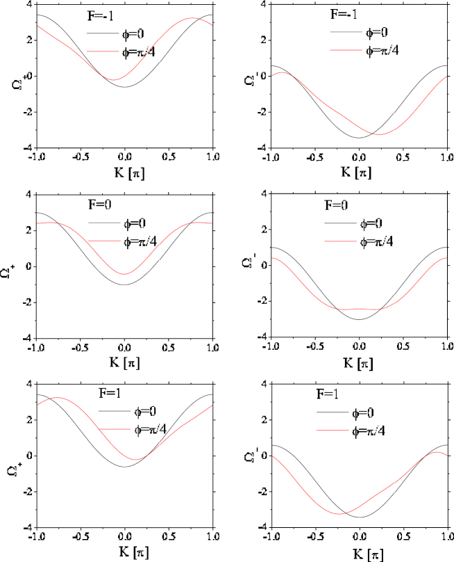
Figure 1: (Color online) Dispersion curves $\Omega(K)$ for the linearized system at different combinations of the values of parameters $F$ and $\phi$, as indicated in the corresponding plots. Other coefficients are $\xi=1$ and $\,g=-1$. The complexes formed of fundamental discrete solitons are expected to exist in the regions with $\Omega<0$ (semi-infinite gaps), i.e., below the black (red) lines, depending on the system’s parameters.

The objective of the work is to construct discrete solitons in this model, and then test their dynamical stability and mobility. Obviously, the solitons must be located inside gaps of the dispersion relation (12), see Fig. 1.

Stationary soliton solutions of Eqs. (5) and (6) were obtained by adopting the nonlinear equation solver based on the Powell method powell . Direct dynamical simulations were based on the Runge-Kutta numerical procedure of the sixth order powell . The numerical solution was performed for a finite lattice, $-N/2\leq p\leq+N/2$, of size $N+1$ with even $N$, and periodic boundary conditions. In this case, the system preserves the total probability, which is normalized to be $1$:

$$P=\sum_{p=-N/2}^{+N/2}(|\Psi_{p}|^{2}+|\Phi_{p}|^{2})\equiv 1,$$ (13)

and the corresponding energy,

$$\left\langle\hat{H}\right\rangle=\frac{1}{2}\sum_{p=-N/2}^{+N/2}\left\{-F\left(\left|\Psi_{p}\right|^{2}-\left|\Phi_{p}\right|^{2}\right)\right.$$

$$-\xi\Psi_{p}^{\ast}\left(\Psi_{p-1}e^{-i\phi}+\Psi_{p+1}e^{i\phi}\right)-\xi\Phi_{p}^{\ast}\left(\Phi_{p-1}e^{i\phi}+\Phi_{p+1}e^{-i\phi}\right)$$

$$\left.+g\Psi_{p}^{\ast}\Phi_{p}+\frac{1}{2}\Delta\omega\left|\Psi_{p}\right|^{2}\left|\Phi_{p}\right|^{2}\right\}+\mathrm{c.c.}$$ (14)

The analysis presented below was performed with $N=101$, unless stated otherwise.

Before proceeding to the description of results, it is relevant to discuss the applicability of the proposed model to really existing QDs. Parameters of an isolated QD, as well as the inter-dot coupling, widely vary depending on the configuration, material and environment of the QD. Coefficients which are used below are realistic for typical semiconductor-based QDs. Firstly, as noted in Ref. 15 , for the observation of the RO modified by the local field effects, it is essential to use an exciting optical pulse with $\Omega\lesssim\Delta\omega$. This implies that one should use an optical pulse which is longer than the Rabi-period, $2\pi/\Omega$, but still sufficiently shorter than transverse damping time, $T_{\mathrm{damp}}$. Such conditions where experimentally realized, in particular, in Ref. 15 (with $T_{\mathrm{damp}}\simeq 2.5$ ns) for the QDs grown in a capped layer. Further, the general condition, $g\sim\xi$, defines a range of the field-QD coupling strength in which the interplay of the Rabi dynamics and interdot tunneling is essential. As shown in Ref. 21 , this condition is realistic in typical experimental situations.

III Results and discussion

III.1 Single-soliton complexes

Stationary solitons with frequency $\Omega$ are looked for in the usual form,

$$\left\{\Psi_{p}(t),\Phi_{p}(t)\right\}=e^{-i\Omega t}\left\{A_{p},B_{p}\right\}.$$ (15)

Two-component single-soliton complexes are composed of single-peak pulses in fields $A_{p}$ and $B_{p}$. Recall that, in the single-component DNLS equation, there are two types of fundamental discrete solitons, stable onsite-centered and unstable intersite-centered ones book . We have found that Eqs. (5) and (6) give rise to two species of stationary single-soliton complexes, in which both components are of the same type, either onsite or intersite. Accordingly, these species are referred to as SOOM (single on-on-site mode) and SIIM (single inter-inter-site mode) solutions, respectively. As concerns the relative sign of the two components, the complexes characterized by

$$\mathrm{sgn}\left\{\mathrm{Re}(A_{p})\mathrm{Re}(B_{p})\right\}=\left\{+1,-1\right\}$$ (16)

are called in-phase and counter-phase configurations, respectively.

Stable stationary solitons and robust breathers found in present model are reported below. Before proceeding to their detailed description, it is relevant to discuss the physical purport of these localized collective excitations. Firstly, we note that Eqs. (5) and (6) are invariant with respect to substitution $i\rightarrow-i,~{}\Psi_{p}\longleftrightarrow\Phi_{p}$. This implies the existence of a set of SIIM and SOOM solutions satisfying conditions $\left|A_{p}\right|=\left|B_{p}\right|$, $\mathrm{Re}\left(A_{p}\right)=\mathrm{Re}\left(B_{p}\right)$, $\mathrm{Im}\left(A_{p}\right)=-\mathrm{Im}\left(B_{p}\right)$. Examples of dynamically stable SOOM solitons, which may be considered as Rabi solitons, are presented at Fig. 2. They are characterized by the conserved energy, see Eq. (14), which includes the contribution from the QD chain proper, and the energy of field-QD interaction. Actually, quasiparticles represented by the Rabi solitons may be considered as artificial RO atoms. Dynamical polarization (8) of such excitations harmonically oscillates at the frequency of the external field. These oscillations do not manifest themselves in observable values (such as induced currents), rather serving for the inner stabilization of the Rabi soliton. The tunneling transitions are able to produce the dc current in the soliton, as per Eq. (9). Its value is proportional to $\sin\phi$, hence it vanishes at $\phi\rightarrow 0$. Further, according to Eq. (10), the inversion vanishes for the stationary Rabi solitons.

The situation is different for the breathing SIIM structures, for which the corresponding spectra feature two lines with frequencies $\nu=\Omega$ and $\nu\approx\Omega/2$, see Fig. 3(d) below. This entails emergence of additional lines in the current spectra. In particular, the resonant line at the external-field frequency transforms into a triplet with frequencies $\nu=\Omega$, $\nu\approx\Omega\pm\Omega/2$. Its physical nature is similar to the well-known Mollow triplet in the resonant fluorescence 1' . The dc current transforms into a low-frequency part of the current spectrum, which partially encloses the resonance line at frequency $\nu=\Omega/2$. The appearance of this spectral feature is stipulated by the asymmetry produced by the phase shift. The physical mechanism of its creation is similar to that for the spectral line at the Rabi frequency in the QD’s RO with spatially broken symmetry, predicted in Ref. 1'' .

III.1.1 The case of $\phi=0$

In the case of $\phi=0\$and $F=0$ [no frequency mismatch, see Eq. (7)], stationary single-soliton complexes are formed of two identical onsite or intersite solitons, which are standard DNLS modes with real probability amplitudes, $\mathrm{Im}(A_{p})=\mathrm{Im}(B_{p})=0$, see Fig. 2(b). Two configurations, in-phase and counter-phase, of each complex differ by the sign of the relative sign of the two components. Families of such complexes are represented by the corresponding $\Delta\omega(\Omega)$ curves in Fig. 2(a). It is relevant to stress that families of the solitons in the present system are characterized by such curves (the nonlinearity coefficient versus the carrier frequency), as the total probability (soliton’s norm) is fixed as per Eq. (13). The situation is opposite in nonlinear optics, where the nonlinearity coefficient is fixed, while the total norm varies, showing the total power of the soliton book . Of course, as concerns actual solutions of the model, these two settings may be transformed into each other by rescaling.

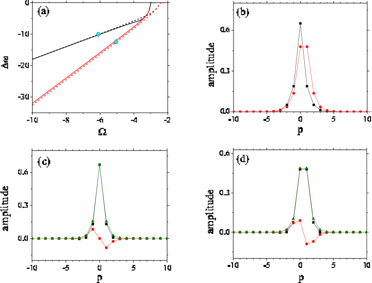
Figure 2: (Color online) (a) The $\Delta\omega$ vs. $\Omega$ diagrams for SOOM and SIIM (black and red line, respectively). Solid lines correspond to $\phi=0$, while dashed ones to $\phi=\pi/4$. (b) Amplitude profiles of onsite components of the SOOM (black) and intersite components of SIIM (red) ($\phi=0$). Plots (c) and (d) show real and imaginary parts (black and red lines) and the absolute value (green) of one component of SOOM and SIIM, respectively, for $\phi=\pi/4$. Note relations $|A_{p}|=|B_{p}|$,  $\mathrm{Re}(A_{p})=\mathrm{Re}(B_{p})$, and $\mathrm{Im}(A_{p})=-\mathrm{Im}(B_{p})$ between the components of these solitons.

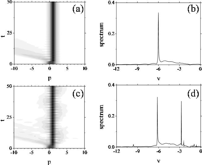
Figure 3: Examples of unstable evolution of SIIM. One of the components is displayed here. (a) The SIIM with $\Omega=-5,\Delta\omega=-11.81$ and $\phi=0$ transforms into an SOOM breather with smaller $\Delta\omega=-10.3$, and $\Omega=-6$ (circles on the curves). The corresponding breather’s spectrum is shown in (b). (c) SIIM with $\Omega=-5,\Delta\omega=-12.32,\phi=\pi/4$ transforms into an onsite breather, whose spectrum is shown in (d).

In accordance with the above-mentioned stability properties of the usual DNLS solitons, only the SOOM of the in-phase type is found to be dynamically stable, while the SIIM evolves, due the instability, into a localized breathing structure. An example of the evolution of an unstable SIIM, with $\Delta\omega=-11.81,\Omega=-5$, into a periodic breather of the SOOM type (with $\Omega\approx-6$) is displayed in Fig. 3. The corresponding spectrum in Fig. 3(c) features one characteristic peak, at $\nu\approx-6$.

Similar behavior is found in the parameter region where the SIIM and SOOM complexes with close values of $\Delta\omega$ coexist [an area of small $|\Omega|$ in Fig. 2(a)]: an unstable SIIM radiates away a small part of its norm and transforms themselves into a SOOM [circles on the respective curves in Fig. 2(a) designate the initial and final states corresponding to the example displayed in Fig. 3(a)]. The spontaneous transformation into a quasi-periodic breather is found too in the region with well separated $\Delta\omega(\Omega)$ curves for different species of the single-soliton complexes. The breathers feature a more complex structure if they develop from the counter-phase original configurations.

III.1.2 The case of $\phi\neq 0$

As said above, the central issue addressed in this work is the novel type of the system of coupled DNLS equations (5) and (6) with $\phi\neq 0$. In this case, the onsite and intersite modes are characterized by complex amplitudes, with $\mathrm{Im}(A_{p}),\mathrm{Im}(B_{p})\neq 0$, see Figs. 2(c) and (d). As in the previous case, the in-phase and counter-phase configurations of the single-soliton modes can be distinguished, as per definition (16). In both configurations, the relative sign of the imaginary parts of the amplitudes is opposite to that for the real parts. Similar to the case of $\phi=0$, only the in-phase SOOMs are stable in the present case, see Fig. 4, while SIIMs develop into breathers of the onsite type, as shown in Figs. 3(c) and (d).

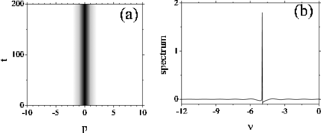
Figure 4: (a) An example of the evolution of the dynamically stable SOOM with $\Omega=-5$, $\Delta\omega=-7.88$ and $\phi=\pi/4$. (b) The corresponding spectrum is characterized by the single line at $\nu=\Omega$.

The presence of the nonzero frequency detuning, $F\neq 0$ [see Eq. (7)] makes the two components of SOOM and SIIM solutions mutually asymmetric. All the findings concerning the dynamical stability of the single-soliton complexes remain the same as for $F=0$. This conclusion turns out to be universal in the framework of the present model, therefore all the results are presented for $F=0$.

Concluding this subsection, we note that systematic simulations demonstrate that moving single-soliton complexes are found in a robust form only in the region where SOOM and SIIM species coexist with nearly equal values of $\Delta\omega$. As usual, the moving modes can be generated, for any value of $\phi$, from stable standing ones by the application of the kick to both components, $\left\{\Psi_{p},\Phi_{p}\right\}\rightarrow e^{iKp}\left\{\Psi_{p},\Phi_{p}\right\}$. However, it is observed that with increasing the values of $\phi$ the moving mode can be trapped by the lattice potential. Physically, this means that the soliton is created in a segment of the QD chain where an additional ramp (linear potential) is applied. Alternatively, the kick may be imparted by an additional nonresonant laser beam shone along the chain. The resulting running solitons seem as breathing complexes traveling across the lattice, see Fig. (5).

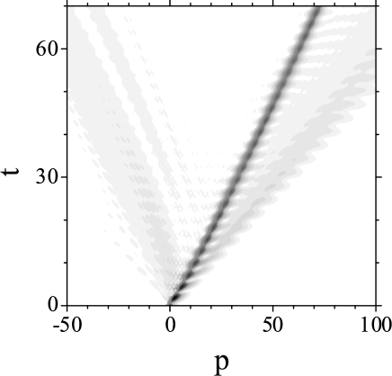
Figure 5: An example of the moving breathing component of the dynamically stable SOOM with $\Omega=-3.6$, $\Delta\omega=-5.86472,\,N=301$ and $\phi=0$. The kick strength is $K=\pi/6$.

III.2 Double soliton complexes

III.2.1 Building bound complexes

The same system of Eqs. (5) and (6) makes it possible to create two-component double-soliton complexes (bound states of fundamental discrete solitons), with two peaks in each component. Stable among them may naturally be double on-on-site modes (DOOMs, i.e., bound states of SOOMs). Here we analyze the dynamics of DOOMs built of two fundamental soliton complexes with the separation between their centers equal to one, three, and five lattice periods ($\Delta=1,3,5$), see Figs. 6 and 9. Depending on the symmetry with respect to the central lattice site, antisymmetric (odd) and symmetric (even) DOOMs can be identified, see Figs. 6 and 9, respectively. In particular, the antisymmetric bound state with $\Delta=1$ corresponds, in the case of the usual single-component DNLS equation, to the well-known twisted modes twisted . Here, we consider only DOOMS of the in-phase type, as concerns the relative phase of the two components, because counter-phase bound states turnout to be strongly unstable.

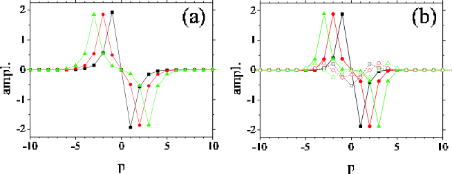
Figure 6: (Color online) (a) The antisymmetric bound state of two onsite solitons (DOOM), with separations $\Delta=1,3,5$ between centers of the solitons, and $\phi=0,\Omega=-5$. (b) The real part (full symbols and solid lines) and imaginary part (empty symbols and dashed lines) for component of the antisymmetric DOOM with $\Omega=-5$ and $\phi=\pi/4$. Black, red and green lines correspond to $\Delta=1,3,5$, respectively

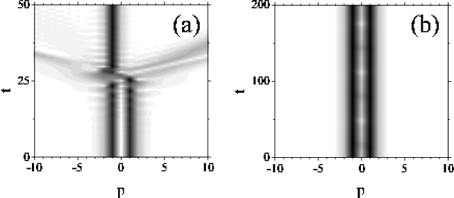
Figure 7: A breathing localized configuration which is a part of the complex formed by perturbing the antisymmetric DOOM with $\Delta=1,\phi=0,\Omega=-5,\Delta\omega=-16.2$ (a), and $\Delta=1,\phi=\pi/4,\Omega=-5,\Delta\omega=-15.7$ (b).

Figure 8: Spectra of the breathers shown in Fig. 7. Plots (a) and (b) show the power spectra at sites $p=-1$ and $p=1$ for $\Delta=1,\phi=0,\Omega=-5,\Delta\omega=-16.2$, which corresponds to Fig. 7(b). Plots (c) shows the spectrum at $p=-1$ for $\Delta=1,\phi=\pi/4,\Omega=-5,\Delta\omega=-15.7$, which corresponds to Fig. 7(b). Both components of the double soliton complexes are identical, therefore the spectra are shown for one of them.

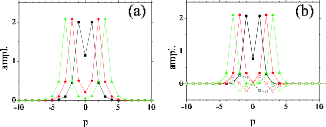
Figure 9: (Color online) (a) The same as in Fig. 6(a) but for a symmetric bound state (DOOM), with $\Omega=-5.8$. (b) The real part (full symbols and solid lines) and imaginary part (empty symbols and dashed lines) for the component of the symmetric DOOM with $\Omega=-5.8$ and $\phi=\pi/4$. Black, red and green lines correspond to $\Delta=1,3,5$.

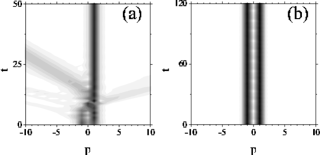
Figure 10: The breather which is part of the complex formed by a perturbed symmetric DOOM with $\Delta=1,\phi=0,\Omega=-5.8$ (a), and $\Delta=1,\phi=\pi/4,\Omega=-5.8$ (b).

III.2.2 The case of $\phi=0$

The amplitudes of the components of the stationary DOOMs in this case are real, as it was the case for SOOMs. Apart from the symmetric DOOM with $\Delta=1$, which is strongly unstable in its whole existence region, complexes of other types are stable, except for narrow instability regions, which shrinks with the increase of separation $\Delta$ between the two solitons. The situation is similar to its well-known counterpart for the single DNLS equation Panos . Examples of the instability development are shown in Figs. 7(a) and 10(a) for antisymmetric and symmetric DOOMs, respectively. To illustrate the structure of the breather which is presented in Fig. 7 (a), its power spectra at sites $p=-1$ and $p=1$ are shown in Fig. 8.

III.2.3 The case of $\phi\neq 0$

In the system with $\phi\neq 0$, both antisymmetric and symmetric DOOMs evolve into bound states of onsite breathers featuring periodic or quasiperiodic oscillations, depending on separation $\Delta$ and parameters of the system, see Figs. 7(b) and 10(b). The spectrum of the on-site breather at site $p=-1$, for the case presented in Fig. 7(b), features a single peak centered close to $\nu=-5$ (not shown here). For other $p$, the corresponding spectra are centered at the same frequency.

IV Conclusions

Our objective in this work was to develop the theory for the interaction of the QD (quantum–dot) chain with classical light in the strong-coupling regime, which takes into account the local-field effect (depolarization). The latter effect makes the system nonlinear. We have introduced the periodic array of identical two-level QDs, coupled via tunneling between neighboring dots. The system of equations of motion has been derived, which includes the tunneling and depolarization. The main conclusions produced by the analysis can be summarized as follows.

(i) The equations of motion have the form of two coupled DNLS (discrete nonlinear Schrödinger) equations for probability amplitudes of the given QD (lattice site) to be found in the ground or excited state. There are two different mechanisms of coupling between the equations. The linear mechanism is stipulated by the “chain-light” interaction, and manifests itself in the form of the RO (Rabi oscillations). The other coupling mechanism is based on the XPM nonlinear terms, which represent the action of the local fields. The constants of the intersite lattice coupling (hopping) are complex ones, whose phases, which are opposite in the two coupled DNLS equations, are determined by the angle between the chain’s axis and the direction of the incident electromagnetic wave. These intersite hopping coefficients, which are complex conjugate to each other in the two equations, represent a drastic difference of the present model from previously studied systems of coupled DNLS equations.

(ii) The numerical analysis has demonstrated that RO waves in the QD chain, coupled to the co-propagating classical electromagnetic field, self-trap into stable onsite-centered fundamental Rabi solitons, while the intersite fundamental solitons are unstable, spontaneously transforming into onsite-centered robust Rabi breathers. Bound states of fundamental solitons are unstable in the stationary state, but they too readily transform themselves into robust breathers. The above-mentioned intersite hopping coefficients, which take complex conjugate in the coupled equations, affect the internal structure of the solitons, making them complex modes, but this novel feature does not destabilize the solitons. The detuning between the light and inter-level transition frequencies breaks the symmetry between the two components of the discrete solitons, but does not affect their stability either. Mobility of the Rabi solitons was investigated too.

(iii) The frequency spectrum of the stable Rabi solitons features a single narrow line at the Rabi frequency. The RO at this frequency do not manifest themselves in terms of observable quantities, serving for the stabilization of the solitons. The inversion of the stable Rabi soliton [$W$, see Eq. (10)] is exactly equal to zero. The frequency spectrum of electric current in the QD chain comprises a narrow line at the external field frequency, as well as the zero-frequency line corresponding to the dc current. The former frequency is produced by the displacement current due to the resonant quantum transitions, while the latter one is induced by the tunneling (intersite hopping).

(iv) The frequency spectrum of the robust Rabi breathers features an additional spectral line, which produces extra lines in the current spectra. The resonant line at the external-field frequency transforms into a triplet, while the dc current transforms into the low-frequency spectral component, which partially overlaps with the single resonance line. The low-frequency current component is induced by the asymmetry, which is determined by the direction of the light propagation relative to the QD chain. Accordingly, the low-frequency component vanishes in the limit of the normal incidence.

The theory presented in this paper does not account for relaxation mechanisms, the quantum structure of the incident light, and interaction of moving Rabi-solitons with edges of the chain (unless the chain is circular, and has no edges). These problems are of special interest and should be considered elsewhere.

- (1) I. I. Rabi, Phys. Rev. 51, 662 (1937).
- (2) H. C. Torrey, Phys. Rev. 76, 1059 (1948).
- (3) G. B. Hocker and C. L. Tang, Phys. Rev. Lett. 21, 591 (1968).
- (4) H. Kamada, H. Gotoh, J. Temmyo, T. Takagahara, and H. Ando, Phys. Rev. Lett. 87, 246401 (2001).
- (5) S. D. Barrett and J. Milburn, Phys. Rev B. 68, 155307 (2003).
- (6) G. Barkard and A. Imamogly, Phys. Rev B. 74, 041307(R) (2006).
- (7) A. Blais, J. Gambetta, A. Wallraff, D. I. Schuster, S. M. Girvin, M. H. Devoret, and R. J. Schoelkopf, Phys. Rev A. 75, 032239 (2007).
- (8) S. Shmitt-Rink, D. A. B. Miller, and D. S. Chemla, Phys. Rev B. 35, 8113 (1987).
- (9) B. Hanewinkel, A. Knorr, P. Thomas, and S. W. Koch, Phys. Rev B. 55, 13715 (1997).
- (10) G. Ya. Slepyan, S. A. Maksimenko, A. Hoffmann, and D. Bimberg, Phys. Rev A. 66, 063804 (2002).
- (11) G. Ya. Slepyan and S. A. Maksimenko, New J. Phys. 10, 023032 (2008).
- (12) G. Ya. Slepyan, A. Magyarov, S. A. Maksimenko, A. Hoffmann, and D. Bimberg, Phys. Rev B. 70, 045320 (2004).
- (13) G. Ya. Slepyan, A. Magyarov, S. A. Maksimenko, A. Hoffmann, Phys. Rev B. 76, 195328 (2007).
- (14) Y. Mitsumori, A. Hasegawa, M. Sasaki, H. Maruki, and F. Minami, Phys. Rev B. 71, 233305 (2005).
- (15) K. Asakara, Y. Mitsumori, H. Kosaka, K. Edamatsu, K. Akahane, N. Yamamoto, M. Sasaki, and N. Ohtani, Phys. Rev B. 87, 241301(R) (2013).
- (16) L. D. Landau and E. M. Lifshitz, Quantum Mechanics (Pergamon Press, 2003).
- (17) Ph. A. Martin and F. Rothen, Many-Body Problems and Quantum Field Theory (Springer-Verlag, Berlin, 2002).
- (18) H. Ajiki, T. Tsuji, K. Kawano, and K. Cho, Phys. Rev B. 66, 245322 (2002).
- (19) M. Lewenstein, L. You, J. Cooper, and K. Burnett, Phys. Rev A. 50, 2207 (1994).
- (20) G. Y. Slepyan, Y. Yerchak, S. A. Maksimenko, and A. Hoffmann, Phys. Lett. A 373, 1374 (2009).
- (21) G. Y. Slepyan, Y. Yerchak, A. Hoffmann, and F. G. Bass, Phys. Rev. B 81, 085115 (2010).
- (22) G. Y. Slepyan, Y. Yerchak, S. A. Maksimenko, A. Hoffmann, and F. G. Bass, Phys. Rev. B 85, 245134 (2012).
- (23) M. Berry, Proc. R. Soc. Lond. A 392, 45 (1964).
- (24) P. G. Kevrekidis, The Discrete Nonlinear Schrödinger Equation: Mathematical Analysis, Numerical Computations, and Physical Perspectives (Springer: Berlin and Heidelberg, 2009).
- (25) M. Johanning, A. F. Varón, and C. Wunderlich, J. Phys. B: At. Mol. Opt. Phys. 42, 154009 (2009).
- (26) G. Herring, P. G. Kevrekidis, B. A. Malomed, R. Carretero-González, and D. J. Frantzeskakis, Phys. Rev. E 76, 066606 (2007).
- (27) M. O. Scully and M. S. Zubairy, Quantum Optics (Cambridge University Press: Cambridge, England, 2001).
- (28) L. Novotny and B. Hecht, Principles of Nano-Optics (Cambridge University Press: New York, 2006).
- (29) A. Maluckov, Lj. Hadžievski, B. A. Malomed, L. Salasnich, Phys. Rev. A 78, 013616 (2008).
- (30) O. V. Kibis, G. Ya. Slepyan, S. A. Maksimenko, and A. Hoffmann, Phys. Rev. Lett. 102, 023601 (2009).
- (31) S. Darmanyan, A. Kobyakov, and F. Lederer, Zh. Eksp. Teor. Fiz. 113, 1253 (1998) [J. Exp. Theor. Phys. 86, 682 (1998)].
- (32) T. Kapitula, P. G. Kevrekidis, and B. A. Malomed, Phys. Rev. E 63, 036604 (2001).