Force spectroscopy of polymer desorption: Theory and Molecular Dynamics simulation

Abstract

Forced detachment of a single polymer chain, strongly-adsorbed on a solid substrate, is investigated by two complementary methods: a coarse-grained analytical dynamical model, based on the Onsager stochastic equation, and Molecular Dynamics (MD) simulations with Langevin thermostat. The suggested approach makes it possible to go beyond the limitations of the conventional Bell-Evans model. We observe a series of characteristic force spikes when the pulling force is measured against the cantilever displacement during detachment at constant velocity $v_{c}$ (displacement control mode) and find that the average magnitude of this force increases as $v_{c}$ grows. The probability distributions of the pulling force and the end-monomer distance from the surface at the moment of final detachment are investigated for different adsorption energy $\epsilon$ and pulling velocity $v_{c}$. Our extensive MD-simulations validate and support the main theoretical findings. Moreover, the simulation reveals a novel behavior: for a strong-friction and massive cantilever the force spikes pattern is smeared out at large $v_{c}$. As a challenging task for experimental bio-polymers sequencing in future we suggest the fabrication of stiff, super-light, nanometer-sized AFM probe.

I Introduction

In recent years single-molecule pulling techniques based on the use of laser optical tweezers (LOT) or atomic force microscope (AFM) have gained prominence as a versatile tool in the studies of non-covalent bonds and self-associating bio-molecular systems Ritort ; Franco ; Hugel ; Butt ; Gao ; Janshof ; Carrion ; Fisher ; Gaub . The latter could be exemplified by the base-pair binding in DNA as well as by ligand-receptor interactions in proteins and has been studied recently by means of Brownian dynamic simulations and the master equation approach Alexander_1 ; Alexander_2 . The LOT and AFM methods are commonly used to manipulate and exert mechanical forces on individual molecules. In LOT experiments, a micron-sized polystyrene or silica bead is trapped in the focus of the laser beam by exerting forces in the range $0.1-100\>pN$. Typically, AFM (which covers forces interval in $20\>pN-10\>nN$ range) is ideal for investigations of relatively strong inter- or intramolecular interactions which are involved in pulling experiments in biopolymers such as polysaccharides, proteins and nucleic acids. On the other hand, due to the relatively small signal-to-noise ratio, the AFM experiments have limitations with regard to the mechanochemistry of weak interactions in the lower piconewton regime.

The method of dynamic force spectroscopy (DFS) is used to probe the force-extension relationship, rupture force distribution, and the force vs loading rate dependence for single-molecule bonds or for more complicated multiply-bonded attachments. Historically, the first theoretical interpretation of DFS has been suggested in the context of single cell adhesion by Bell Bell and developed by Evans Evans_1 ; Evans_2 ; Evans_3 . The consideration has been based on the semi-phenomenological Arrhenius relation which describes surface detachment under time-dependent pulling force, $f=r_{l}t$, with $r_{l}$ being the loading rate. It was also assumed that the effective activation energy, $E_{b}(f)$, may be approximated by a linear function of the force, i.e., $E_{b}(f)=E_{b}^{(0)}-x_{\beta}f$. Here $x_{\beta}$ is the distance between the bonded state and the transition state where the activation barrier is located. The resulting Bell-Evans (BE) equation then gives the mean detachment force as a function of temperature $T$ and loading rate $r_{l}$, i.e., $f=\frac{k_{B}T}{x_{\beta}}\ln(\frac{rx_{\beta}}{k_{B}T\kappa_{0}})$, where $\kappa_{0}$ is the desorption rate in the absence of applied pulling force.

As one can see from this BE-equation, the simple surmounting of BE-activation barrier results in a linear dependence of detachment force on the logarithm of loading rate, provided one uses the applied force as a governing parameter in the detachment process (i.e., working in an isotensional ensemble when $f$ is controlled and the distance $D$ from the substrate to the clamped end-monomer of the polymer chain fluctuates). For multiply-bonded attachments the interpretation problem based on this equation becomes more complicated since a non-linear $f-\ln r_{l}$ relationship is observed Merkel . In this case chain detachment involves passages over a cascade of activation barriers. For example, Merkel et al. Merkel suggested that the net rate of detachments can be approximated by a reciprocal sum of characteristic times, corresponding to jumps over the single barriers. In particular, regarding the detachment of biotin-streptavidin single bonds, it was suggested that two consecutive barriers might be responsible for the desorption process.

A simple example of multiply-bonded bio-assembly is presented by a singe-stranded DNA (ssDNA) macromolecule, strongly adsorbed on graphite substrate. The forced-induced desorption (or peeling) of this biopolymer has been studied analytically and by means of Brownian dynamics (BD) simulation by Jagota et al. Jagota_1 ; Jagota_2 ; Jagota_3 ; Jagota_4 . In ref. Jagota_1 the equilibrium statistical thermodynamics of ssDNA forced-induced desorption under force control (FC) and displacement control (DC) has been investigated. In the latter case one works in an isometric ensemble where $D$ is controlled and $f$ fluctuates. It has been demonstrated that the force response under DC exhibits a series of spikes which carry information about the underlying base sequence of ssDNA. The Brownian dynamics (BD) simulations Jagota_2 confirmed the existence of such force spikes in the force-displacement curves under DC.

The nonequilibrium theory of forced desorption has been developed by Kreuzer et al. Kreuzer_1 ; Kreuzer_2 ; Kreuzer_3 on the basis of Master Equation approach for the cases of constant velocity and force-ramp modes in an AFM-experiment. The authors assumed that individual monomers detachments represent a fast process as compared to the removal of all monomers. This justifies a two-state model where all monomers either remain on the substrate or leave it abruptly. The corresponding transition rates (which constitute a necessary input in the Master Equation approach) must satisfy detailed balance. As a result of the Master Equation solution, the authors obtained a probability distribution of detachment heights (i.e., distances between the cantilever tip and the substrate) as well as an average detachment height as a function of the pulling velocity.

Irrespective of all these efforts, a detailed theoretical interpretation of the dynamic force spectroscopy experiments is still missing. For example, in terms of Kramers reaction-rate theory Hanggi the Arrhenius-like BE - model holds only when the effective activation energy $E_{b}(f)\gg k_{B}T$. On the other hand, it is clear that for large forces (which we experience in AFM), the case when $E_{b}(f)\approx k_{B}T$ occurs fairly often. In this common case the general approach, based on the BE-model, becomes questionable. Besides, it can be shown Hanke , that the activation energy vs force dependence, $E_{b}(f)$, is itself a nonlinear function, so that the conventional BE - model, based on the linear approximation, $E_{b}(f)\approx E_{b}^{(0)}-x_{\beta}f$, should be limited to small forces. Moreover, the Arrhenius - like relationship for the detachment rate, which was used in the BE - model, is a consequence of a saddle-point approximation for the stationary solution of Fokker- Planck equation Hanggi . This contradicts the typical loading regimes, used in experiments, where applied force or distance grow linearly with time.

The present paper is devoted to the theoretical investigation of a single molecule desorption dynamics and aimed at interpretation of AFM - or LOT - based dynamic force spectroscopy in the DC constant-velocity mode. The organization of the paper is as follows: in Sec. II we give the equilibrium theory of detachment for the case of strong polymer adsorption. The mean force (measured at the cantilever tip) versus displacement diagram is discussed in detail. In particular, the characteristic force-“spikes” structure (which was first discussed in Ref. Jagota_1 ; Jagota_2 ) can be clearly seen. In Sec. III we give a dynamical version of the detachment process. Our approach rests on construction of general free energy functions, depending on coarse-grained variables, which govern the non-linear response and structural bonding changes in presence of external forces. The corresponding free-energy-based stochastic equations (known as Onsager equations Puri ) are derived and solved numerically. This solution makes it possible to provide not only force-displacement diagrams and the ensuing dependence on cantilever displacement velocity $v_{c}$ but also the detachment force probability distribution function (PDF). In Sec. IV the main theoretical results are then checked against extensive Molecular Dynamics (MD) simulation. A brief discussion of results is offered in Sec. V.

II Equilibrium theory at the strong adsorption case

Figure 1: Principal scheme of a single molecule forced desorption experiment based on the AFM: (left panel) There is no friction between the adsorbed portion and substrate. (right panel) Strong friction case.

Recently we suggested a theory of the force-induced polymer desorption (for relatively weak adsorption energy) in the isotensional Bhattacharya_1 ; Bhattacharya_2 and isometric Bhattacharya_3 equilibrium ensembles supported by extensive Monte Carlo (MC) simulations. In the former case, the fraction of adsorbed monomers changes abruptly (undergoes a jump) when one varies the adsorption energy or the external pulling force. In the second case, the order parameter varies steadily with changing height of the AFM-tip, even though the phase transition is still of first order. The total phase diagram in terms of adsorption energy - pulling force, or, adsorption energy - end-monomer height, has been discussed theoretically and in terms of MC-simulations.

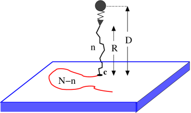
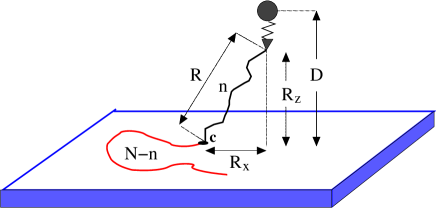
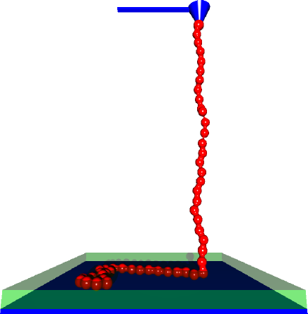
On the other hand, the AFM experiments deal with relatively strong forces ($20\>pN-10\>nN$ Ritort ) so that in the case of a single molecule desorption experiment only a really strong adsorption energy is essential. This limit has been discussed in the recent papers by Jagota et al. Jagota_1 ; Jagota_2 ; Jagota_3 ; Jagota_4 and Kreuzer ey al. Kreuzer_1 ; Kreuzer_2 ; Kreuzer_3 . Here we consider this problem in a slightly more general form. In so doing we distinguish between two different models: with frictionless- and strong-friction substrates, as indicated in Fig. 1.

II.1 Frictionless substrate

This case has been considered in Refs. Jagota_1 ; Jagota_2 ; Kreuzer_1 ; Kreuzer_2 ; Kreuzer_3 and is based on the assumption that the force resisting sliding is sufficiently small, i.e., the cantilever tip and the contact point $c$ are both placed along the same $z$-axis (see Fig. 1 (left panel)). The total partition function for a fixed cantilever distance $D$, i.e., $\Xi_{\rm tot}(D)$, is a product of partition functions of the adsorbed part , $\Xi_{\rm ads}(n)$ , of the desorbed portion (a stretched polymer portion), $\Xi_{\rm pol}(n,R)$, and of the cantilever itself, $\Xi_{\rm can}(D-R)$, where $n$ is the number of desorbed polymer segments, and $R$ denotes the distance between the clamped end of this desorbed portion and the substrate. As a result,

$$\Xi_{\rm tot}(D)=\sum_{n=0}^{N}\>\Xi_{\rm ads}(n)\>\int\limits_{0}^{bn}\>dR\;\Xi_{\rm pol}(n,R)\>\theta(D-R)\Xi_{\rm can}(D-R),$$ (1)

where the integration interval, $0<R<bn$, and the step-function, $\theta(D-R)$, imply that restrictions, $R<bn$ and $R<D$, should be applied simultaneously. In this representation $D$ is the control variable (which is monitored by the corresponding AFM operating mode) whereas $n$ and $R$ are coarse-grained dynamic variables which should be integrated (in our case, an integral over $R$, and summation over $n$) out. Moreover, if we introduce the function

$$\min(bn,D)=\begin{cases}bn&\mbox{for}\qquad bn<D\\ D&\mbox{for}\qquad D<bn,\end{cases}$$ (2)

then Eq. (1) can be rewritten as

$$\Xi_{\rm tot}(D)=\sum_{n=0}^{N}\>\Xi_{\rm ads}(n)\>\int\limits_{0}^{\min(bn,D)}\>dR\;\Xi_{\rm pol}(n,R)\>\Xi_{\rm can}(D-R)$$ (3)

In the strong adsorption regime, $\Xi_{\rm ads}(n)$ attains a simple form

$$\Xi_{\rm ads}(n)=\exp\left[\epsilon(N-n)\right],$$ (4)

where the dimensionless adsorption energy $\epsilon=\varepsilon/k_{B}T$. The cantilever manifests itself as a harmonic spring with a spring constant $k_{c}$, i.e., the corresponding partition function reads

$$\Xi_{\rm can}(D-R)=\exp\left[-\dfrac{k_{c}}{2k_{B}T}(D-R)^{2}\right]$$ (5)

Finally, we derive the partition function of the desorbed part of the polymer as function of the dynamic variables $n$ and $R$, based of the Freely Jointed Bond Vector (FJBV) model Lai ; Schurr . The corresponding Gibbs free energy (i.e., the free energy in the isotensional-ensemble) is

$$G_{\rm pol}(n,{\widetilde{f}})=-nk_{B}T\>\ln\left[\dfrac{\sinh{\widetilde{f}}}{{\widetilde{f}}}\right],$$ (6)

where the dimensionless force ${\widetilde{f}}\stackrel{{\scriptstyle\rm def}}{{=}}bf/k_{B}T$. The corresponding distance $R=-\partial G_{\rm pol}(n,{\widetilde{f}})/\partial{\widetilde{f}}$.

$$R=-\dfrac{\partial G_{\rm pol}}{\partial f}=nb{\cal L}({\widetilde{f}}),$$ (7)

where the so called Langevin function ${\cal L}({\widetilde{f}})\equiv\coth({\widetilde{f}})-1/{\widetilde{f}}$ has been used. In the isometric-ensemble, the proper thermodynamic potential is the Helmholtz free energy, $F_{\rm pol}(n,R)$, which is related to $G_{\rm pol}(n,{\widetilde{f}})$ by Legendre transformation,

$$F_{\rm pol}(n,R)=G_{\rm pol}(n,{\widetilde{f}})+f\>R,$$ (8)

where $f=\partial F_{\rm p}(n,R)/\partial R$. Taking the Gibbs free energy, Eq. (6), into account and the relation Eq. (7) for the Helmholtz free energy, we have

$$F_{\rm pol}(n,R) = G_{\rm pol}(n,{\widetilde{f}})+f\>R$$ (9)

$$= -n\>k_{B}T\>\ln\left[\dfrac{\sinh{\widetilde{f}}}{{\widetilde{f}}}\right]+{\widetilde{f}}\>k_{B}T\>n\>{\cal L}({\widetilde{f}})$$

$$= -n\>k_{B}T\;\left\{\ln\left[\dfrac{\sinh{\widetilde{f}}}{{\widetilde{f}}}\right]+1-{\widetilde{f}}\>\coth({\widetilde{f}})\right\}\equiv-n\>k_{B}T\;{\cal G}({\widetilde{f}}),$$

where the function ${\cal G}(x)\equiv\ln[\sinh(x)/x]+1-x\coth(x)$. As a result, Eq. (9) along with Eq. (7) parametrically define $F_{\rm p}(n,R)$, and the corresponding partition function

$$\Xi_{\rm pol}(n,R)=\exp\left[n{\cal G}({\widetilde{f}})\right]$$ (10)

as function of $n$ and $R$.

By making use of Eqs. (4), (5), (10), the total partition function given by Eq. (1) reads

$$\Xi_{\rm tot}(D)=\sum_{n=0}^{N}\>\int\limits_{0}^{\min(nb,D)}\>dR\;\exp\left[\epsilon(N-n)\right]\>\exp\left[n\>{\cal G}({\widetilde{f}})\right]\>\exp\left[-\dfrac{k_{c}}{2k_{B}T}(D-R)^{2}\right].$$ (11)

In Eq. (11) the force ${\widetilde{f}}$ should be expressed in terms of $R/bn$ as follows: ${\widetilde{f}}={\cal L}^{-1}(R/bn)$, where ${\cal L}^{-1}(x)$ denotes the inverse Langevin function. The corresponding effective free energy function in terms of $n$ and $R$ reads

$${\cal F}(n,R)=-k_{B}T\epsilon(N-n)-k_{B}Tn{\cal G}({\widetilde{f}})+\dfrac{k_{c}}{2}\left(D-R\right)^{2}$$ (12)

In the limit of a very stiff cantilever, $k_{c}b^{2}/k_{B}T\gg 1$, the cantilever partition function approaches a $\delta$-function Kreuzer_1 :

$$\Xi_{\rm can}(D-R)=\exp\left[-\dfrac{k_{c}}{2k_{B}T}(D-R)^{2}\right]\rightarrow(2\pi k_{B}T/k_{c})^{1/2}\>\delta(D-R),$$ (13)

and Eq. (11) takes the form

$$\Xi_{\rm tot}(D)=\sum_{n=0}^{N}\>\exp\left[\epsilon(N-n)\right]\>\exp\left[n\>{\cal G}({\widetilde{f}})\right]\>\theta(nb-D),$$ (14)

where ${\widetilde{f}}={\cal L}^{-1}(D/bn)$ and the step-function $\theta(bn-D)$ ensures that the condition $bn>D$ holds. It is this very stiff cantilever limit that was considered in ref. Jagota_1 ; Jagota_2 .

For the isometric ensemble, i.e., in the $D$-ensemble, the average force $\langle f_{z}\rangle$, measured by AFM-experiment, is given by

$$\langle f_{z}\rangle = -k_{B}T\>\dfrac{\partial}{\partial D}\>\ln\Xi_{\rm tot}(D)$$ (15)

$$= \dfrac{k_{c}}{\Xi_{\rm tot}(D)}\>\sum_{n=0}^{N}\>\exp\left[\epsilon(N-n)\right]\>\int\limits_{0}^{\min(bn,D)}\>dR\;(D-R)\>\exp\left[n\>{\cal G}({\widetilde{f}})\right]\>\exp\left[-\dfrac{k_{c}}{2k_{B}T}(D-R)^{2}\right],$$

where $\Xi_{\rm tot}(D)$ is given by Eq. (11).

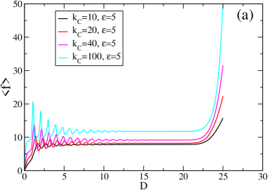
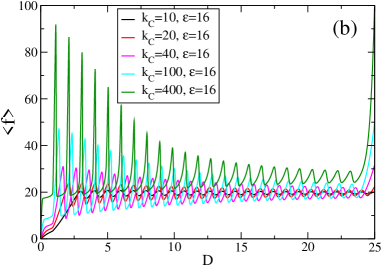
The numerical results, which follow from Eq. (15), are shown in Fig. 2. One can immediately see the ”sawtooth“-, or force-spikes structure on the force-displacement diagram as it was also found by Jagota et al. Jagota_1 in the limit of very stiff cantilever. Physically, spikes correspond to the reversible transitions $n\rightleftarrows n+1$, during which the release of polymer stretching energy is balanced by the adsorption energy. The corresponding thermodynamic condition reads ${\cal F}(n,R)={\cal F}(n+1,R)$. This condition also leads to the spikes amplitude law $f_{\rm amp}\propto\exp(\epsilon/n)$ Jagota_1 , i.e. the spikes amplitude gradually decreases in the process of chain detachment (i.e., with growing $n$).

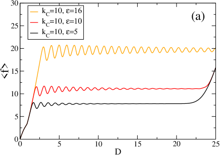
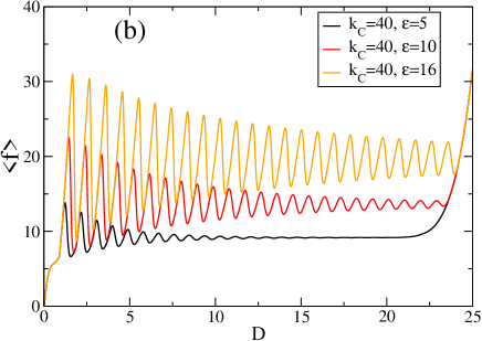
This structure is more pronounced at larger adsorption energy $\epsilon$ and cantilever spring constant $k_{c}$. Thus, while the force oscillates, its mean value remains nearly constant in a broad interval of distances $D$, exhibiting a kind of plateau. Complementary information (for fixed $k_{c}$ at different values of $\epsilon$) is given on Fig. 3. One can verify that the plateau height is mainly determined by $\epsilon$ whereas the spikes amplitude is dictated by the cantilever spring constant $k_{c}$.

Figure 2: The equilibrium force-displacement diagrams calculated according to Eq. (15). The sawtooth structure becomes more pronounced with increasing adsorption energy $\epsilon$ and spring constant $k_{c}$.

Figure 3: The equilibrium force-displacement diagrams calculated according to Eq.  (15). The same as in Fig. 2 but for fixed $k_{c}$ and different $\epsilon$.

II.2 Strong polymer-substrate friction

In this limit one has to take into account the specific geometry of an AFM experiment, shown in Fig. 1 (right panel). For simplicity, an infinite friction of the polymer at the surface is assumed. The adsorbed polymer portion may be considered as a two-dimensional self-avoiding chain comprising $N-n$ segments. The last contact point (marked as $c$ in Fig. 1) can move due to adsorption or desorption elementary events. In Ref. Netz this was classified as the sticky case. In Fig. 1, $D$ is the distance from the cantilever base to to the substrate, $R_{z}$ is the height of the cantilever tip above the substrate, and $R$ is the distance between the cantilever tip and the contact point $c$. Eventually, $R_{x}$ is the lateral distance between cantilever base and the contact point $c$. One may assume that initially the desorbed portion of $n$ segments has occupied a distance of $R_{x}$ which, due to self-avoiding $2D$-configurations of an adsorbed chain, equals $R_{x}^{2}\approx b^{2}n^{2\nu}$ (where $\nu=3/4$).

The specific geometry of the AFM experiment in the case of strong polymer-substrate friction (shown in Fig. 1) brings about changes only in the cantilever partition function, i.e., instead of Eq. (5), one has

$$\Xi_{\rm can}(D,R) = \exp\left[-\dfrac{k_{c}}{2k_{B}T}(D-R_{z})^{2}\right].$$ (16)

$$= \exp\left[-\dfrac{k_{c}}{2k_{B}T}\left(D-\sqrt{R^{2}-b^{2}n^{2\nu}}\right)^{2}\right]$$

As a result, the total partition function in this case is given by

$$\Xi_{\rm tot}(D)=\sum_{n=0}^{N}\>\exp\left[\epsilon(N-n)\right]\>\int\limits_{bn^{\nu}}^{bn}\>dR\;\exp\left[n\>{\cal G}({\widetilde{f}})\right]\>\exp\left[-\dfrac{k_{c}}{2k_{B}T}\left(D-\sqrt{R^{2}-b^{2}n^{2\nu}}\right)^{2}\right]\theta(D-\sqrt{R^{2}-b^{2}n^{2\nu}})$$ (17)

where again the variable ${\widetilde{f}}$ should be excluded in favor of $R/bn$ by means of the relation ${\widetilde{f}}={\cal L}^{-1}(R/bn)$. In Eq. (17) the following constraints

$$bn^{\nu} < R<bn,$$

$$R_{z} = \sqrt{R^{2}-b^{2}n^{2\nu}}<D,$$ (18)

have been taken into account.

The corresponding free energy functional in terms of dynamical variables $n$ and $R$ has the following form

$${\cal F}(n,R)=-k_{B}T\epsilon(N-n)-k_{B}Tn{\cal G}({\widetilde{f}})+\dfrac{k_{c}}{2}\left(D-\sqrt{R^{2}-b^{2}n^{2\nu}}\right)^{2}.$$ (19)

The average force, which is measured in AFM-experiments, is given by

$$\langle f_{z}\rangle=\dfrac{k_{c}}{\Xi_{\rm tot}(D)}\>\sum_{n=0}^{N}\>\>\int\limits_{bn^{\nu}}^{bn}\>dR\;\left(D-\sqrt{R^{2}-b^{2}n^{2\nu}}\right)\>\> \exp\left[\epsilon(N-n)+n\>{\cal G}({\widetilde{f}})-\dfrac{k_{c}}{2k_{B}T}\left(D-\sqrt{R^{2}-b^{2}n^{2\nu}}\right)^{2}\right]$$ (20)

$$\times\theta\left(D-\sqrt{R^{2}-b^{2}n^{2\nu}}\right).$$

III Dynamics of desorption

In our recent paper Paturej we have studied a single polymer force-induced desorption kinetics by making use of the notion of tensile blobs as well as by means of Monte Carlo and Molecular Dynamics simulations. It was clearly demonstrated that the total desorption time $<\tau_{d}>$ scales with polymer length $N$ as $<\tau_{d}>\propto N^{2}$.

In order to treat a realistic AFM experiment in which the cantilever-substrate distance changes with constant velocity $v_{c}$, i.e., $D(t)=D_{0}+v_{c}t$, one has to consider the AFM tip dynamics. With this in mind, we will develop a coarse-grained stochastic model based on the free-energy functional Eq. (12). Before proceeding any further, we need to define the adsorption-desorption potential profile $F_{\rm ads}(n)$. This plays the role of the potential of mean force (PMF) which depends on $n$.

III.1 Stochastic Model

In the Helmholtz free-energy functional ${\cal F}(n,R)$, given by Eq. (12) and Eq. (19), the free energy of the adsorbed portion is given by a simple contact potential, $F_{\rm ads}=-k_{B}T\epsilon(N-n)$, where $n$ is an integer number in the range $0\leq n\leq N$. Considering desorption dynamics (see below), we will treat $n$ as a continuous variable with a corresponding adsorption-desorption energy profile satisfying the following conditions:

1. For integer $n$-values the energy profile has minima whereby we use the contact potential $F_{\rm ads}(n)=-k_{B}T\epsilon(N-n)$.

2. For half-integer values of $n$ the adsorption potential goes over maxima.

3. The activation barrier for monomer desorption, $\Delta E^{+}=F_{\rm ads}(n+1/2)-F_{\rm ads}(n)$, and the corresponding adsorption activation barrier, $\Delta E^{-}=F_{\rm ads}(n+1/2)-F_{\rm ads}(n+1)$, are proportional to the adsorption strength $\epsilon$ of the substrate whereby $\Delta E^{+}>\Delta E^{-}$.

4. The adsorption-desorption energy profile satisfies the boundary conditions: $F_{\rm ads}(0)=-k_{B}T\epsilon N$ (a fully adsorbed chain), and $F_{\rm ads}(N)=0$ (an entirely detached chain).

One may show that the following energy profile, given as

$$F_{\rm ads}(n)=T\epsilon\left\{1+\cos[(2n+1)\pi]+n\right\}-k_{B}T\epsilon N,$$ (21)

meets the conditions (1) - (4).

The minima and maxima of Eq. (21) are located in the points defined by $\sin[(2s+1)\pi]=1/2\pi$ with $s$ denoting the continuous index of a monomer.

Figure 4: Adsorption-desorption potential profiles for two different strengths $\epsilon=5$ and $\epsilon=10$ of surface attraction. The integer $n$-values correspond to minima whereas at half-integer $n$-values the potential has local maxima. The dashed lines denote the corresponding contact potential $F_{\rm ads}=-\varepsilon(N-n)$ which has been used in Sec. II.

As a result,

$$s=\begin{cases}\dfrac{1}{2\pi}\arcsin\left(\dfrac{1}{2\pi}\right)+k-\dfrac{1}{2}&\mbox{for}\quad k=1,2,\dots\\ \\ -\dfrac{1}{2\pi}\arcsin\left(\dfrac{1}{2\pi}\right)+n&\mbox{for}\quad n=0,1,2,\dots\end{cases}$$ (22)

In Eq. (22) the first term, $(1/2\pi)\arcsin(1/2\pi)\approx 0.025$, is very small and could be neglected. Thus, the minima and maxima are located at the integer and half integer points respectively (see Fig. 4)

In order to calculate the activation barriers, we determine first $F_{\rm ads}(s)$ at the half-integer points, i.e.,

$$F_{\rm ads}(n+1/2)=k_{B}T\epsilon(n+5/2)-k_{B}T\epsilon N,$$ (23)

as well as at the integer points

$$F_{\rm ads}(n) = k_{B}T\epsilon n-k_{B}T\epsilon N$$

$$F_{\rm ads}(n+1) = k_{B}T\epsilon(n+1)-k_{B}T\epsilon N.$$ (24)

Therefore, the activation barriers for the detachment, $\Delta E^{+}$, and adsorption, $\Delta E^{-}$, are given by

$$\Delta E^{+} = F_{\rm ads}(n+1/2)-F_{\rm ads}(n)=\dfrac{5}{2}k_{B}T\epsilon$$

$$\Delta E^{-} = F_{\rm ads}(n+1/2)-F_{\rm ads}(n+1)=\dfrac{3}{2}k_{B}T\epsilon$$ (25)

i.e., $\Delta E^{+}>\Delta E^{-}$. Finally, one may readily see that $F_{\rm ads}(0)=-k_{B}T\epsilon N$ and $F_{\rm ads}(N)=0$ which is in line with condition (iv).

The total Helmholtz free energy for the frictionless substrate model is given by

$${\cal F}(n,R)=k_{B}T\epsilon\left\{1+\cos[(2n+1)\pi]+n\right\}-k_{B}T\epsilon N-k_{B}Tn{\cal G}({\widetilde{f}})+\dfrac{k_{c}}{2}\left(D-R\right)^{2},$$ (26)

whereas for the strong polymer-substrate friction model we have

$${\cal F}(n,R)=k_{B}T\epsilon\left\{1+\cos[(2n+1)\pi]+n\right\}-k_{B}T\epsilon N-k_{B}Tn{\cal G}({\widetilde{f}})+\dfrac{k_{c}}{2}\left(D-\sqrt{R^{2}-b^{2}n^{2\nu}}\right)^{2}.$$ (27)

These Helmholtz free energy functions govern the dissipative process which is described by the stochastic (Langevin) differential equations

$$\dfrac{\partial n}{\partial t} = -\lambda_{n}\>\dfrac{\partial}{\partial n}\>{\cal F}(n,R)+\xi_{n}(t)$$

$$\dfrac{\partial R}{\partial t} = -\lambda_{R}\>\dfrac{\partial}{\partial R}{\cal F}(n,R)+\xi_{R}(t)$$ (28)

where $\lambda_{n}$ and $\lambda_{R}$ are the Onsager coefficients. The random forces $\xi_{n}(t)$ and $\xi_{R}(t)$ describe Gaussian noise with means and correlators given by

$$\langle\xi_{n}(t)\rangle = \langle\xi_{R}(t)\rangle=0$$

$$\langle\xi_{n}(t)\xi_{n}(0)\rangle = 2\lambda_{n}k_{B}T\delta(t)$$

$$\langle\xi_{R}(t)\xi_{R}(0)\rangle = 2\lambda_{R}k_{B}T\delta(t)$$ (29)

Equations (28) are usually referred to as the Onsager equations Puri .

The set of stochastic differential equations, Eq.(28) can be treated by a time integration scheme. Each realization $(l)$ of the solution provides a time evolution of $n^{(l)}(t)$ and $R^{(l)}(t)$. In order to get mean values of the observables, these trajectories should be averaged over many independent runs $l=1,2,\dots\cal N$. For example, in order to obtain the average force, Eq. (20), one should average over the runs

$$\langle f_{z}(t)\rangle=\dfrac{k_{c}}{\cal N}\>\sum_{l=1}^{\cal N}\>\left(D(t)-\sqrt{[R^{(l)}(t)]^{2}-b^{2}[n^{(l)}(t)]^{2\nu}}\right)$$ (30)

III.2 Thermodynamic forces

The thermodynamic forces which arise in Eq. (28), i.e., $f_{n}\stackrel{{\scriptstyle\rm def}}{{=}}-\frac{\partial{\cal F}(n,R}{\partial n}$ and $f_{R}\stackrel{{\scriptstyle\rm def}}{{=}}-\frac{\partial{\cal F}(n,R)}{\partial R}$, could be calculated explicitly. For example, for the free energy function, Eq. (26), one has

$$f_{n} = -k_{B}T\epsilon\left\{1-2\pi\sin[(2n+1)\pi]\right\}+k_{B}T\>{\cal G}({\widetilde{f}})+k_{B}T\>n\>{\cal G}^{\prime}({\widetilde{f}})\>\left(\dfrac{\partial{\widetilde{f}}}{\partial n}\right)_{R}$$ (31)

$$= -k_{B}T\epsilon\left\{1-2\pi\sin[(2n+1)\pi]\right\}+k_{B}T\>{\cal G}({\widetilde{f}})-\dfrac{k_{B}T\>R}{b\>n}\>\dfrac{{\cal G}^{\prime}({\widetilde{f}})}{{\cal L}^{\prime}({\widetilde{f}})},$$

where we have used (recall that $R/bn={\cal L}({\widetilde{f}})$)

$$\left(\dfrac{\partial{\widetilde{f}}}{\partial n}\right)_{R}=-\dfrac{R/bn^{2}}{{\cal L}^{\prime}({\widetilde{f}})}.$$

On the other hand, a direct calculation shows that

$${\cal G}^{\prime}(x) = \dfrac{x}{[\sinh(x)]^{2}}\>-\>\dfrac{1}{x}$$

$${\cal L}^{\prime}(x) = \dfrac{1}{x^{2}}\>-\>\dfrac{1}{[\sinh(x)]^{2}}$$ (32)

so that

$$\dfrac{{\cal G}^{\prime}(x)}{{\cal L}^{\prime}(x)}=-x.$$ (33)

Thus, for the force $f_{n}$, given by Eq. (31), one has

$$f_{n}=-k_{B}T\epsilon\left\{1-2\pi\sin[(2n+1)\pi]\right\}+k_{B}T\dfrac{R\>{\widetilde{f}}}{b\>n}+k_{B}T\>{\cal G}({\widetilde{f}}).$$ (34)

In the strong friction case, Eq. (27) leads to a more complicated expression for the thermodynamic force:

$$f_{n}=-k_{B}T\epsilon\left\{1-2\pi\sin[(2n+1)\pi]\right\}+k_{B}T\dfrac{R\>{\widetilde{f}}}{b\>n}+k_{B}T\>{\cal G}({\widetilde{f}})+\>\nu\;b^{2}\>k_{c}\;\left(\dfrac{D}{\sqrt{R^{2}-b^{2}n^{2\nu}}}-1\right).$$ (35)

For $f_{R}\stackrel{{\scriptstyle\rm def}}{{=}}-\partial{\cal F}(n,R)/\partial R$ one obtains

$$f_{R}=k_{B}T\>n\>{\cal G}^{\prime}({\widetilde{f}})\>\left(\dfrac{\partial{\widetilde{f}}}{\partial R}\right)_{n}+k_{c}(D-R)=\dfrac{k_{B}T}{b}\>\dfrac{{\cal G}^{\prime}({\widetilde{f}})}{{\cal L}^{\prime}({\widetilde{f}})}\>+\>k_{c}(D-R)$$ (36)

where we have used

$$\left(\dfrac{\partial{\widetilde{f}}}{\partial R}\right)_{n}=\dfrac{1/bn}{{\cal L}^{\prime}({\widetilde{f}})}.$$

Taking into account Eq. (33), one finally derives

$$f_{R}=-\dfrac{k_{B}T\>{\widetilde{f}}}{b}\>+\>k_{c}(D-R).$$ (37)

For the model, given by Eq. (27), the corresponding force reads

$$f_{R}=-\dfrac{k_{B}T\>{\widetilde{f}}}{b}\>+\>k_{c}\;R\>\left(\dfrac{D}{\sqrt{R^{2}-b^{2}n^{2\nu}}}-1\right).$$ (38)

Finally, the variable ${\widetilde{f}}$ should be expressed in terms of $R/bn$ by making use of the relationship ${\widetilde{f}}={\cal L}^{-1}(R/bn)$, where ${\cal L}^{-1}(x)$ is the inverse Langevin function. A very good approximation for the inverse Langevin function, published in Ref. Cohen , is given by

$${\widetilde{f}}={\cal L}^{-1}(R/bn)\approx \dfrac{R}{bn}\>\left[\dfrac{3-\left(\dfrac{R}{bn}\right)^{2}}{1-\left(\dfrac{R}{bn}\right)^{2}}\right]$$ (39)

III.3 Quasistationary approximation

It could be shown that for a strongly stretched desorbed portion of the polymer chain, the $R$ variable rapidly relaxes to its quasi-stationary value (see Appendix A). In other words, $R$ can quickly adjust to the slow evolution of $n$ (governed by the Kramers process). In this quasi-stationary approximation $f_{R}=0$, and from Eq. (37) one has $k_{c}(D-R)=k_{B}T{\widetilde{f}}/b$, so that the following nonlinear equation for $R$ emerges

$$k_{c}[D(t)-R]=\dfrac{k_{B}T}{b}\>{\cal L}^{-1}\left(\frac{R}{nb}\right)$$ (40)

This could be represented as

$$G(n,R;t)\stackrel{{\scriptstyle\rm def}}{{=}}\dfrac{R}{bn}-{\cal L}\left(\dfrac{k_{c}b[D(t)-R]}{k_{B}T}\right)=0,$$ (41)

i.e., the height $R$ is instantaneously coupled to the number of desorbed beads, $n$. Inserting Eq. (39) into Eq. (40), one obtains

$$P(n,R;t)\stackrel{{\scriptstyle\rm def}}{{=}}\dfrac{k_{c}b[D(t)-R]}{k_{B}T}-\left(\dfrac{R}{bn}\right)\>\left[\dfrac{3-\left(\dfrac{R}{bn}\right)^{2}}{1-\left(\dfrac{R}{bn}\right)^{2}}\right]=0.$$ (42)

The Onsager equation for the slow variable $n$ is given as

$$\dfrac{\partial n}{\partial t} = \lambda_{n}\>f_{n}(n,R)+\xi_{n}(t)$$ (43)

$$= \lambda_{n}\>[-k_{B}T\epsilon\left\{1-2\pi\sin[(2n+1)\pi]\right\}+k_{B}T\dfrac{R\>{\widetilde{f}}}{b\>n}+k_{B}T\>{\cal G}({\widetilde{f}})]+\xi_{n}(t)$$

where ${\widetilde{f}}$ is determined by Eq. (39).

Eventually, we get a system of so-called semi-explicit differential-algebraic equations (DAE) Ascher

$$\dfrac{\partial n}{\partial t} = \lambda_{n}\>f_{n}(n,R)+\xi_{n}(t)$$

$$0 = G(n,R;t)$$ (44)

In this particular form of DAE one can distinguish between the differential variable $n(t)$ and the algebraic variable $R(t)$. Eq. (44) can be solved numerically by making use of an appropriate Runge - Kutta (RK) algorithm, as shown in the Appendix B.

III.4 Results

Figure 5: (left panel) The effect of averaging over many desorption events. The blue line shows a single run, whereas the red line demonstrates the result of averaging over $300$ runs. The detachment velocity $v_{c}=100$, the cantilever spring $k_{c}=100$, adsorption energy $\epsilon=5$, and the Onsager coefficient $\lambda=0.1$. (right panel) The dynamic force-displacement diagram for $\epsilon=5$ and different detachment velocities $v_{c}$ (see legend).

We have solved numerically our stochastic model, given by Eq. (43) and Eq. (41), for the case of frictionless substrate. To this end we used the second order Runge - Kutta (RK) algorithm for stochastic differential-algebraic equations (see Appendix B for more details). The advantage of the stochastic differential equations approach as compared to the Master Equation method Kreuzer_3 is that the former one gives a more detailed (not averaged) dynamic information corresponding to each individual force-displacement trajectory (as is often in an experiment). The result of averaging over $300$ runs is shown in Fig. 5 (left).

Fig. 5 (right panel) shows the resulting force - displacement diagram for $\epsilon=5$ and different detachment velocities. It it worth noting that the ”sawtooth” pattern can be seen for all investigated detachment velocities ranging between $v_{c}=5\times 10^{-4}$ and $v_{c}=10^{-2}$. For larger velocities the plateau height of the force grows substantially. In other words, the mean detachment force increases as the AFM-tip velocity gets higher and the bonds stretching between successive monomers becomes stronger.

Figure 6: The normalized PDF for detachment forces at $\epsilon=5$ (a), and $\epsilon=8$ (b), as well as for different detachment velocities $v_{c}$ (shown in the legends). The PDFs for the detachment distance $R$ of cantilever tip at $\epsilon=5$ (c) and $\epsilon=8$ (d).

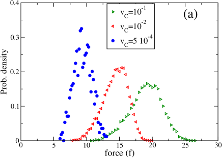
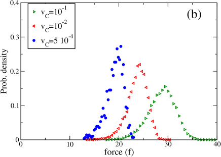
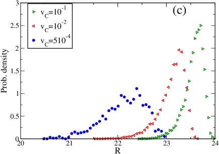
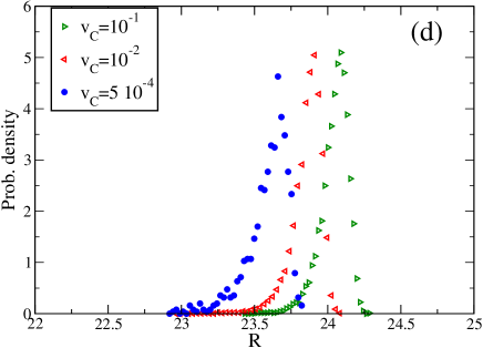
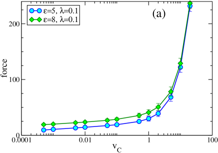
We have also studied the detachment force behavior as well as that of the cantilever tip distance from the substrate at the moment of a full detachment, (i.e. when $n=N$), by repeating the detachment procedure $10^{4}$ times and plotting the probability distribution functions (PDF) for different adsorption energies $\epsilon$ and detachment velocities $v_{c}$ - Fig. 6. As one can see from Fig. 6a, b, both the average and the dispersion of detachment force grow with $v_{c}$ which agrees with findings for reversible (i.e., when a broken bond can rebind) bond-breaking dynamics Diezemann . In contrast, the mean cantilever tip distance $R$ variance decreases and its average value increases with growing $v_{c}$ (cf. Fig. 6c, d).

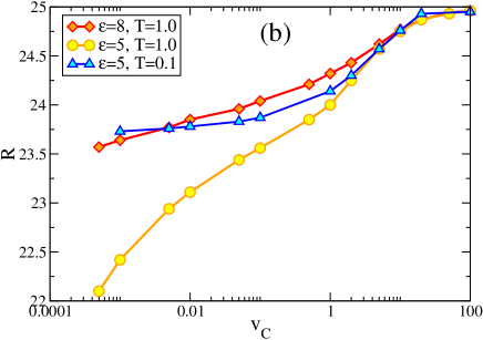
The average detachment force dependence on cantilever velocity $v_{c}$ is a widely covered subject in the literature in the context of biopolymers unfolding Kreuzer_4 ; Eom_1 ; Eom_2 or forced separation of two adhesive surfaces Leckband ; Seifert ; Diezemann . Figure 7a, which shows the result of our calculations, has the characteristic features discussed also in ref. Leckband . One observes a well expressed crossover from a shallow-slope for relatively small detachment rates to a steep-slope region as detachment speed increases. One remarkable feature is that this crossover practically does not depend on the adsorption energy $\epsilon$: the curve is merely shifted upwards upon increasing of $\epsilon$. Therefore, the crossover is not related to a competition between the Kramers rate and the cantilever velocity but rather accounts for the highly nonlinear chain stretching as the velocity $v_{c}$ increases. The corresponding detachment distance of the cantilever tip $R$ (detachment height), Fig. 7b, reveals a specific sigmoidal shape in agreement with the results based on the Master Equation Kreuzer_3 . At low velocities of pulling, $v_{c}$, when the chain still largely succeeds in relaxing back to equilibrium during detachment, an interesting entropy effect is manifested in Fig. 7b: the (effectively) stiffer coil at $T=1.0$ leaves the substrate at lower values of $R$ than in the case of the colder system, $T=0.1$. As the pulling velocity grows, however, this entropic effect vanishes and the departure from the substrate is largely governed by the stretching of the bonds rather than of the coil itself whereby the difference in behavior between $T=1.0$ and $T=0.1$ disappears.

Figure 7: The average detachment force (a), and cantilever tip distance (b), vs detachment velocity $v_{c}$ for two different adsorption energies $\epsilon=5$ and $\epsilon=8$. In addition, the distance $R$ is plotted in (b) for two different temperatures, $T=1.0$ and $T=0.1$, both at the same adsorption strength $\epsilon=5.0$. Evidently, with growing $T$ the elasticity of the coil decreases, the coil itself becomes stiffer and therefore detaches from the substrate at lwoer height $R$. This entropic effect is well expressed at sufficiently low pulling velocity only.

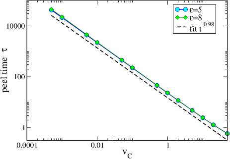
Eventually, as it can be seen from Fig. 8, the total detachment (peel) time $\tau_{\rm det}$ vs. velocity $v_{c}$ relationship has a well-defined power-law behavior, $\tau_{\rm det}\sim 1/v_{c}^{\alpha}$, with the power $\alpha\approx 1$, in line with previous theoretical findings Seifert .

Figure 8: The average detachment (peeling) time $\tau_{\rm det}$ versus detachment velocity $v_{c}$ for two different adsorption energies $\epsilon=10$ and $\epsilon=16$. The inversely proportional dependence, $\tau_{\rm det}\sim 1/v_{c}$, agrees well with previous theoretical findings Seifert .

IV MD simulations

IV.1 The model

In our MD-simulations we use a coarse-grained model of a polymer chain of $N$ beads connected by finitely extendable elastic bonds. The bonded interactions in the chain is described by the frequently used Kremer-Grest potential, $V^{\mbox{\tiny KG}}(r)=V^{\mbox{\tiny FENE}}(r)+V^{\mbox{\tiny WCA}}(r)$. The FENE (finitely extensible nonlinear elastic) potential is given by

$$V^{\mbox{\tiny FENE}}=-\frac{1}{2}kr_{0}^{2}\ln{\left[1-\left(\frac{r}{r_{0}}\right)^{2}\right]}$$ (45)

with $k=30\,\epsilon/\sigma^{2}$ and $r_{0}=1.5\sigma$.

In order to allow properly for excluded volume interactions between bonded monomers, the repulsion term is taken as Weeks-Chandler-Anderson (WCA) potential (i.e., the shifted and truncated repulsive branch of the Lennard-Jones potential,) given by

$$V^{\mbox{\tiny WCA}}(r)=4\epsilon\left[(\sigma/r)^{12}-(\sigma/r)^{6}+1/4\right]\theta(2^{1/6}\sigma-r)$$ (46)

with $\theta(x)=0$ or $1$ for $x<0$, or $x\geq 0$, and $\epsilon=1$, $\sigma=1$. The overall potential $V^{\mbox{\tiny KG}}(r)$ has a minimum at bond length $r_{\mbox{\tiny bond}}\approx 0.96$. The nonbonded interaction between monomers are taken into account by means of the WCA potential, Eq. 46. Thus, the interactions in our model correspond to good solvent conditions.

The substrate in the present investigation is considered simply as a structureless adsorbing plane, with a Lennard-Jones potential acting with strength $\epsilon_{s}$ in the perpendicular $z$–direction, $V^{\mbox{\tiny LJ}}(z)=4\epsilon_{s}[(\sigma/z)^{12}-(\sigma/z)^{6}]$. In our simulations we consider as a rule the case of strong adsorption $\epsilon_{s}/k_{B}T=5\div 20$, where $k_{B}T$ is a temperature of Langevin thermal bath described below.

The dynamics of the chain is obtain by solving the Langevin equations of motion for the position $\mathbf{r}_{n}=[x_{n},y_{n},z_{n}]$ of each bead in the chain,

$$m\ddot{\mathbf{r}}_{n}=\mathbf{F}_{n}^{j}+\mathbf{F}_{n}^{\mbox{\tiny WCA}}-\gamma\dot{\mathbf{r}}_{n}+\mathbf{R}_{n}(t)\qquad(1,\ldots,N)$$ (47)

which describes the Brownian motion of a set of bonded particles.

The influence of solvent is split into slowly evolving viscous force and rapidly fluctuating stochastic force. The random Gaussian force $\mathbf{R}_{n}$ is related to friction coefficient $\gamma=0.25$ by the fluctuation-dissipation theorem. The integration step is $\tau=0.005$ and time in measured in units of $\sqrt{m\sigma^{2}/\epsilon}$, where $m$ denotes the mass of the polymer beads, $m=1$. In all our simulations the velocity-Verlet algorithm was used to integrate equations of motion (47).

Figure 9: Snapshots of a polymer chain with $N=50$ monomers during detachment from a substrate at $\varepsilon=2.5$ (left) and $\varepsilon=20$ (right). Here $v_{c}=0.0001$. The interaction range of the adsorption potential is shaded (transparent) green. The cantilever tip is shown schematically in blue. One may clearly see that the polymer chain is more relaxed (less stretched) at $\varepsilon=2.5$, and the adsorbed monomers do not stick tightly to the surface but partially exit the range of surface adsorption.

The molecule is pulled by a cantilever at constant velocity $\mathbf{V}=[0,0,v_{c}]$. The cantilever is imitated by two beads connected by harmonic spring and attached to one of the ends of the chain.

The mass of beads $m_{c}$, forming the cantilever, was set either to $m_{c}=1$ or to $25$. The equilibrium size of this harmonic spring was set to $0$ and the spring constant was varied in the range $k_{c}=50\div 400\,\epsilon/\sigma^{2}$. The hydrodynamics radius $a$ of beads composing the cantilever was varied by changing the friction coefficient $\gamma_{c}=0.25\div 25$, taking into account the Stokes’ law, $\gamma_{c}=6\pi\eta a$, where $\eta$ is the solvent viscosity.

Taking the value of the thermal energy $k_{B}T\approx 4.11\times 10^{-21}$ J at $k_{B}T=300$ K, the typical Kuhn length of $\sigma=1$ nm and the mass of coarse-grained monomer as $m\approx 10^{-25}$ kg setups the unit of time in our simulations which is given in $~{}10^{-12}\,{\text{s}}=1$ ps. The velocities used in simulations are in units of $10^{-4}\div 10^{-1}\,\text{nm}/\text{ps}\approx 10^{-1}\div 10^{2}\,\text{m}/\text{s}$. Spring constants of our cantilever in real units are: $k_{c}=50\div 400\,k_{B}T/(\text{nm})^{2}=0.2\div 1.6\,\text{N}/\text{m}$.

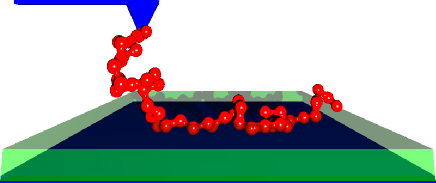
Two typical snapshots of a polymer chain during slow detachment from an adsorbing substrate with different strengths of adsorption, $\varepsilon=2.5$ and $\varepsilon=20$ are shown in Fig. 9. Evidently, the chain is much more stretched for the strongly-attractive substrate where all adsorbed monomers stick firmly to the surface.

Figure 10: Comparison of averaged force measured at the cantilever vs single realization of desorption experiment. Force $f$ at the cantilever was calculated by monitoring extensions $\Delta z_{c}$ of a harmonic spring, i.e. $f=k_{c}\Delta z_{c}$. Here $N=20$, $k_{c}=50\,\epsilon/\sigma^{2}$, $v_{c}=10^{-4}\,\sigma/\tau$ and $\epsilon_{s}/k_{B}T=20$. $m_{c}=1$ and $\gamma_{c}=0.25$.

IV.2 MD-results

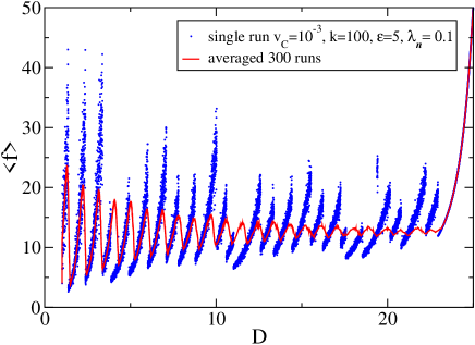
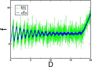
As we have already seen in Sec. III.4, the averaging of the force profile over many runs reveals the inherent sawtooth-structure of the force vs distance dependence (see Fig. 5) which is otherwise overshaded by thermal noise. Our MD-simulation result, depicted in Fig. 10, show the same tendency against the noisy background of a single detachment event. Therefore, for better clarity and physical insight, all our graphic results that are given below result from such averaging procedure.

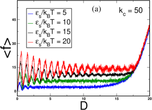
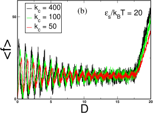
Figure 11a shows how adsorption energy $\epsilon$ affects the force $f$ vs distance $D$ relationship. Apparently, with increasing $\epsilon$ the mean force (plateau height) is found to grow in agreement with our equilibrium theory results, given in Fig. 3. As suggested by our recent theory Bhattacharya_1 ; Bhattacharya_3 , the plateau height goes up as $f_{p}\propto\epsilon^{1/2}$, or as $f_{p}\propto\epsilon$, for relatively small or large $\epsilon$ values, respectively. The amplitude of spikes increases with growing $\epsilon$ too, in line with the equilibrium findings (see Fig. 3). Moreover, as found by Jagota et al. Jagota_1 , the amplitude of spikes follows an exponential law, $f_{\rm amp}\propto\exp(\epsilon/n)$, where $n$ is the number of desorbed polymer segments. On the other hand, the comparison of Fig. 11b and Fig.2 suggests that the stiffness of the cantilever spring constant $k_{c}$ affects mainly the spike amplitude especially at large $\epsilon$.

Figure 11: Time-averaged force $\langle f\rangle$ at the cantilever as a function of a distance from the substrate $D$ during chain detachment. Here $N=20$, $v_{c}=10^{-4}\,\sigma/\tau$, $m_{c}=1$ and $\gamma_{c}=0.25$. Presented results are for different adsorption strengths $\epsilon$, as indicated in the legend, and $k_{c}=50\epsilon/\sigma^{2}$ (a). Figure (b) presents results for $\epsilon=20$ and different spring constants $k_{c}$. Each curve originates from $10^{3}$ independent simulations.

Figure 12: Profiles of averaged force $\langle f\rangle$ vs distance above the substrate $D$ displayed for different pulling velocities $v_{c}$ . Here $N=20$, $k_{c}=50\,\epsilon/\sigma^{2}$ and $\epsilon_{s}/k_{B}T=20$ and (a) $m_{c}=1,\gamma_{c}=1$ , (b) $m_{c}=1,\gamma_{c}=25$, (c) $m_{c}=25,\gamma_{c}=0.25$, (d) $m_{c}=25,\gamma_{c}=25$.

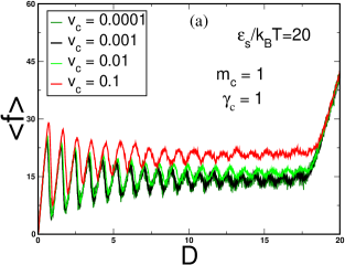
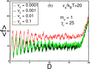
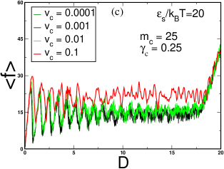
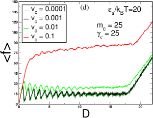
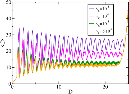
Eventually, we demonstrate the impact of cantilever velocity, $v_{c}$, as well as of its mass, $m_{c}$, and friction coefficient, $\gamma_{c}$, on the force-distance profile. Apparently, these parameters affect differently strong the observed force - distance relationship. Similar to the results, obtained for our coarse-grained model in Sec. II, in the MD-simulation data the plateau height grows less than twice upon velocity increase of three orders of magnitude (see Fig. 12)! Only for a very massive, ($m_{c}=25$), and strong-friction, ($\gamma_{c}=25$), cantilever, the plateau height grows significantly and gains a slight positive slope (see Fig.12d) whereby oscillations vanish. This occurs for the fastest detachment $v_{c}=0.1$. Evidently, this effect is related to the combined role of the friction force in the case of rapid detachment along with the much larger inertial force ($m_{c}=25$) whereby the substrate-induced oscillations are overshadowed by the increased effort of pulling. In contrast, neither Fig. 12b, nor Fig. 12c indicate any major qualitative changes in the $f$-vs-$D$-behavior when medium-friction, or mass cantilever alone are drastically changed.

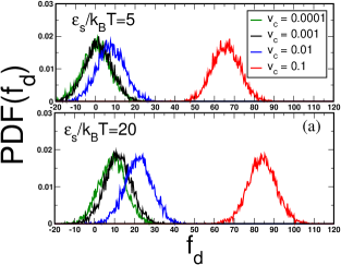
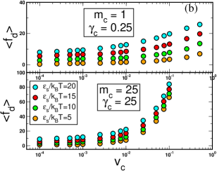
The PDF of the detachment force and its velocity $v_{c}$ dependence are shown in Fig. 13. Similarly as in Sec. II, the average value and dispersion grow with increasing speed of pulling and this is weakly sensitive with regard to the adsorption strength of the substrate $\epsilon$. Remarkably, the mean detachment force $\langle f_{d}\rangle$ shows a similar nonlinear dependence on $\ln v_{c}$ (cf. Fig. 7a). The crossover position does not change practically as the adhesion strength is varied, and the variation of the other parameters ($m_{c}=1\to 25,\;\gamma_{c}=0.25\to 25$) towards a massive and strong-friction cantilever render this crossover considerably more pronounced.

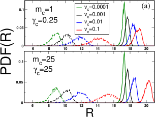
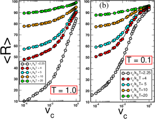
The complementary PDF for the detachment height $R$ is given in Fig. 14a together with the corresponding average $\langle R\rangle$ vs $v_{c}$ relationship. As predicted by our analytic model, cf. Section II, the height of final detachment of the chain from the substrate becomes larger for faster peeling $v_{c}$ and stronger adhesion $\epsilon$, which is consistent with the MD data. One can see again the typical sigmoidal-shape in the $\langle R\rangle$ vs $v_{c}$ dependence.

The two panels for different temperature, shown in Fig. 14b, indicate a smaller increase in $\langle R\rangle$ at the higher temperature, provided the pulling velocity $v_{c}$ is sufficiently small too. This can be readily understood in terms entropic (rubber) elasticity of polymers and represents a case of delicate interplay between entropy and energy-dominated behavior. It is well known that a polymer coil becomes less elastic (i.e., it contracts) upon a temperature increase, cf. the lowest (grey) curve in Fig. 14b, (left panel) at $T=1.0$, so that $R$ is smaller than in the corresponding lowest curve for $T=0.1$ in the right panel of Fig. 14b. This occurs at low values of $v_{c}$. On the other hand, the softer chain (at $T=0.1$) stretches more easily and, therefore, $R$ goes up to $\approx 95$ for the highest speed $v_{c}=10^{4}$ instead of $R\approx 80$ for $T=1.0,v_{c}=10^{4}$. This entropic effect is well expressed at weak attraction to the surface, $\epsilon/k_{B}T=2.25$, which does not induce strong stretching of the bonds along the chain backbone. In contrast, at high $\epsilon/k_{B}T=20$, the bonds extend so strongly that the chain turns almost into a string and entropy effects become negligible. The energy cost of stretching then dominates and leads to higher values of $R$ at the higher temperature (cf. upper most green symbols in Fig. 14b) since it is now the elasticity of the bonds between neighboring segments which governs the physics of detachment. In this case the elastic constant of the bonds effectively decreases with an increase of $T$ so that the distance of detachment $R$ in the left panel of Fig. 14b for $T=1.0$ is higher than that for $T=0.1$ in the right panel.

Figure 13: (a) Probability distribution function of a force $f_{d}$ at the cantilever measured in the moment of detachment (when the last monomer leaves the substrate). Here $N=20$, $k_{c}=50\,\epsilon/\sigma^{2}$ , $\epsilon_{s}/k_{B}T=20$, $m_{c}=1$ and $\gamma_{c}=0.25$. (b) Averaged force $\langle f_{d}\rangle$ plotted versus pulling velocity $v_{c}$ in the semilogaritmic scale. The values of parameters are the same.

Figure 14: (a) Probability distribution function of the detachment height $R$. Upper panel present results for $m_{c}=1$ and $\gamma_{c}=0.25$ while lower panel contains data for $m_{c}=25$ and $\gamma_{c}=25$. Solid line represent results for $\epsilon_{s}/k_{B}T=20$ while dashed line for $\epsilon_{s}/k_{B}T=5$. Here $N=20$, $k_{c}=50\,\epsilon/\sigma^{2}$. (b) Averaged detachment height $\langle R\rangle$ as a function of pulling velocity $v_{c}$ in the semi-logarithmic scale plotted for different adsorption strengths as indicated: (left panel) $k_{B}T=1.0$, (right panel) $k_{B}T=0.1$. On both panels symbols plotted with same color correspond to the same ratio of $\epsilon_{s}/k_{B}T$ while the corresponding values of $\epsilon_{s}$ and $k_{B}T$ differ. Here $N=100$, $k_{c}=50\,\epsilon/\sigma^{2}$, $m_{c}=1$ and $\gamma_{c}=0.25$.

V Discussion

We have demonstrated in this paper that a simple theory, based on the Onsager stochastic equations, yields an adequate description of a typical AFM- experiment within the displacement-control mode. This approach makes it possible to relax most of the restrictions inherent in the BE-model. For example, this approach also holds for small desorption activation barriers (i.e., for $E_{b}(f)\approx k_{B}T$), and also for nonlinear barrier vs. force dependence. It naturally takes into account the reversible desorption-adsorption events Diezemann which are neglected in BE-model. Moreover, it does not rest on the stationary approximation (which is customary in the standard Kramers rate calculation Hanggi ) and is, therefore, ideally suited for description of driven force- (FC) or displacement-control (DC) regimes. One of the principal results in this analytic treatment is the predicted existence of characteristic spikes the mean force vs distance profile, observed in the DC-regime. These spikes depend on the adsorption energy $\epsilon$, cantilever spring constant $k_{c}$ as well as on the cantilever velocity $v_{c}$. In equilibrium, this has been found earlier by Jagota and coworkers Jagota_1 . The PDF of detachment forces and detachment distances are been thoroughly investigated. The relevant mean detachment force is found to be a strongly nonlinear function of $v_{c}$ which is mainly governed by the nonlinear chain stretching upon increasing $v_{c}$. The average full detachment (peeling) time scales $\propto 1/v_{c}$ which is supported by early theoretical findings Seifert .

Some of these predictions were checked by means of MD-simulation and found in a qualitative agreement with the results, gained by the analytic method. Most notably, this applies to properties like the characteristic force oscillations pattern and the mean force vs cantilever velocity $v_{c}$ dependence. On the other hand, our MD-simulation reveals a very strong increase in the magnitude of the force plateau for a strong-friction ($\gamma_{c}=25$) and massive ($m_{c}=25$) cantilever. Interestingly, in this case the spikes pattern is almost totally smeared out. This might be the reason why the force spikes pattern is not seen in laboratory detachment experiments. We recall that in a recent Brownian dynamic simulation (which totally ignores inertia forces) Jagota_3 , the friction coefficient of the cantilever was $70$ times larger than the friction coefficient of the chain segments. It was shown that for this high-friction cantilever and large velocity of pulling, the force spikes pattern was significantly attenuated Jagota_3 so that information on the base sequence was hardly assessable. Therefore, fabrication of a stiff and super-light, nanometer-sized AFM probe would be a challenging task for future developments of biopolymer sequencing.

As an outlook, our coarse-grained Onsager stochastic model could be generalized to encompass investigations of forced unfolding of a multi-domain, self-associating biopolymers Kreuzer_4 .

Acknowledgement

This work was supported by grant SFB 625 from German Research Foundation (DFG). Computational time on PL-Grid Infrastructure is acknowledged. A.M. thanks the Max Planck Institute for Polymer Research in Mainz, Germany, and CECAM - MPI for hospitality during his visit at the Institute.

Appendix A The separation $R$ as an instantaneously adjustable variable

Due to strong adsorption, the desorbed portion of polymer chain is expected to be strongly stretched. One could simplify the force, $f_{R}\approx(R/bn)[3-(R/bn)^{2}]/[1-(R/bn)^{2}]\approx 1/[1-(R/bn)]$, where Eq. (39) has been used and the contribution of the cantilever has been neglected. Therefore, the simplified equation which governs $R$ reads

$$\dfrac{dR}{dt}\approx-\dfrac{\lambda_{R}k_{B}T}{b[1-(R/bn)]}$$ (48)

This equation can be easily solved and the corresponding solution has the form

$$\dfrac{1-R(t)/bn}{1-R_{0}/bn}=\sqrt{1+t/\tau_{R}}$$ (49)

where the relaxation time $\tau_{R}=(b^{2}/2k_{B}T\lambda_{R})(1-R_{0}/bn)^{2}$. This result suggests that for a strongly stretched chain, i.e., for $R_{0}\leqslant bn$, the relaxation time $\tau_{R}$ is very small Febbo . For example, in the case that $R_{0}=b(n-1)$ we have

$$\tau_{R}=\dfrac{b^{2}}{2k_{B}T\lambda_{R}n^{2}}$$ (50)

This relaxation time should be compared to the characteristic time, $\tau_{\rm Kram}$, of the slow variable $n(t)$ which is governed by the Kramers process. According to the semi-phenomenological Bell model Bell , the characteristic time of unbonding (that is, desorption in our case) is given by $\tau_{\rm Kram}=\tau_{0}\exp[(\Delta E-r_{0}f_{p})/k_{B}T]$ where $\tau_{0}=\xi_{0}b^{2}/k_{B}T$ is the segmental time, $\Delta E=F_{1}-F_{2}$ is the activation energy for single monomer desorption, $r_{0}$ stands for the width of adsorption potential, and $f_{p}$ is the plateau height. The free energies in the desorbed, $F_{1}$, and in the adsorbed, $F_{2}$, states are given by $F_{1}=-k_{B}T\ln\mu_{2}$ and $F_{2}=-k_{B}T\epsilon-k_{B}T\ln\mu_{3}$ where $\mu_{2}$ and $\mu_{3}$ are the so-called connective constants in two- and three dimensions respectively Vanderzande .

As mentioned in Sec. IV.2, for large adsorption energies $\epsilon$ the dimensionless plateau height ${\widetilde{f}}_{p}\stackrel{{\scriptstyle\rm def}}{{=}}bf_{p}/k_{B}T\propto\epsilon$. Taking this into account, one could represent $\tau_{\rm Kram}$ in the following form:

$$\tau_{\rm Kram}=\dfrac{\tau_{0}\mu_{2}}{\mu_{3}}\>\exp[(1-\alpha)\epsilon],$$ (51)

where $\alpha=r_{0}/b<1$. Therefore, in the case when $\tau_{R}\ll\tau_{\rm Kram}$, the distance $R$ could be treated as the fast variable. With Eqs. (50) and (51) and taking into account that the Onsager coefficient $\lambda_{R}=1/\xi_{0}n$, this condition means that

$$\dfrac{n\mu_{2}}{\mu_{3}}\>\exp[(1-\alpha)\epsilon]\gg 1.$$ (52)

This condition holds for all typical values of the relevant parameters.

Appendix B Runge-Kutta algorithm for stochastic differential-algebraic equations

In order to solve the DAE (44) numerically, one may employ the second order Runge-Kutta (RK) algorithm. To this end the first equation in Eq. (44) may be rewritten as an integral equation which relates the $i$-th and $i+1$ grid points (using discrete time points $t_{i}=ih$)

$$n_{i+1}=n_{i}+\lambda_{n}\int\limits_{t_{i}}^{t_{i+1}}\>f_{n}(n(s),R(s))ds+w_{n}(h)$$ (53)

where $h$ is the time step and $n_{i}=n(ih)$. Moreover, $w_{n}(h)=\int_{t_{i}}^{t_{i+1}}\;\xi_{n}(s)ds$ describes a Wiener process with zero mean and with variance:

$$\langle w_{n}(h)w_{n}(h)\rangle = \int_{t_{i}}^{t_{i+1}}ds_{1}\;\int_{t_{i}}^{t_{i+1}}ds_{2}\langle\xi_{n}(s_{1})\xi_{n}(s_{2})\rangle=2\lambda_{n}k_{B}T\>\int_{t_{i}}^{t_{i+1}}ds_{1}\;\int_{t_{i}}^{t_{i+1}}ds_{2}\;\delta(s_{1}-s_{2})$$ (54)

$$= 2\lambda_{n}k_{B}T\>h$$

The integral over the deterministic force in Eq. (53) within this $2-nd$ order approximation reads

$$\int_{t_{i}}^{t_{i+1}}\>f_{n}(n(s),R(s))\>ds\approx\dfrac{h}{2}\left[f_{n}(n_{i+1},R_{i+1})+f_{n}(n_{i},R_{i})\right]+{\cal O}(h^{3})$$ (55)

This is so-called trapezoidal rule for approximation of the integral. In order to calculate $f_{n}(n_{i},R_{i})$, one should first take the initial value $n_{i}$, and find $R_{i}$ through the solution of the nonlinear equation $G(n_{i},R_{i},t_{i})=0$. For the calculation of $f_{n}(n_{i+1},R_{i+1})$, one can use the forward Euler method of order $1$, i.e., $n_{i+1}^{E}=n_{i}+h\lambda_{n}f_{n}(n_{i},R_{i})+h^{1/2}(2\lambda_{n}k_{B}T)^{1/2}Z_{n}$ and $R_{i+1}^{E}$ are obtained as solution of the equation $G(n_{i+1}^{E},R_{i+1}^{E},t_{i+1})=0$. Here the random variable $Z_{n}$ is Gaussian with zero mean value and with variance

$$\langle Z_{n}^{2}\rangle=1$$ (56)

As a result, the recursive procedure which relates the $i$-th and $i+1$ grid points can be defined as:

1. For a given initial value of $n_{i}$, go to Eq. (41) or Eq. (42) and solve this nonlinear equation (e.g. $G(n_{i},R_{i},t_{i})=0$) with respect to $R_{i}$.

2. Compute $g_{1}=f_{n}(n_{i},R_{i})$.

3. Compute $n_{i+1}$ and $R_{i+1}$ within the Euler approximation, i.e., calculate first $n_{i+1}^{E}=n_{i}+h\lambda_{n}f_{n}(n_{i},R_{i})+h^{1/2}(2\lambda_{n}k_{B}T)^{1/2}Z_{n}$ and then solve $G(n_{i+1}^{E},R_{i+1}^{E},t_{i+1})=0$ with respect to $R_{i+1}^{E}$.

4. Compute $g_{2}=f_{n}(n_{i+1}^{E},R_{i+1}^{E})$.

5. Compute the corrected $n_{i+1}$ , i.e.

   $$n_{i+1}=n_{i}+\dfrac{h}{2}(g_{1}+g_{2})+h^{1/2}(2\lambda_{n}k_{B}T)^{1/2}Z_{n}$$

6. Finally, with the value of $n_{i+1}$, go to item $1$ and solve the nonlinear equation $G(n_{i+1},R_{i+1},t_{i+1})=0$ with respect to $R_{i+1}$.

References

- (1) F. Ritort, J. Phys.: Condens. Matter, 2006, 18, R531 - R583.
- (2) I. Franco, M.A. Ratner, G.C. Schatz, Single-Molecule Pulling: Phenomenology and Interpretation, in Nano and Cell Mechanics: Fundamentals and Frontiers, edited by H.D. Esinosa and G. Bao (Wiley, Microsystem and Nanotechnology Series, 2013) Chap. 14, p. 359-388 .
- (3) B.N. Balzer, M. Gallei, M.V. Hauf, M. Stallhofer, L. Wiegleb, A. Holleiner, M. Rehahn, T. Hugel, Angew. Chem. Int. Ed., 2013, 52, 6541-6544.
- (4) H.-J. Butt, B. Cappella, M. Kappl, Surf. Sci. Rep., 2005, 59, 1-152.
- (5) Y. Gao, G. Sirinakis, Y. Zhang, J. Am. Chem. Soc., 2011, 133, 12749-12757.
- (6) A. Janshof, M. Neitzert, Y. Oberdorfer, H. Fuchs, Angew. Chem., Int. Ed., 2000, 39, 3212 - 3237.
- (7) M. Carrion-Vazquez, A. F. Oberhauser, S. Fowler, P. E. Marszalek, S.E. Broedel, J. Clarke, J. M. Fernandez, Proc. Natl, Acad. Sci. U.S.A., 1999, 96, 3694 - 3699 .
- (8) T. E. Fisher, A. F. Oberhauser, M. Carrion-Vazquez, P. E. Marszalek, J. M. Fernandez, Trends Biochem. Sci., 1999, 24, 379 - 384.
- (9) H. Clausen-Schaumann, M. Seitz, R. Krautbauer, H. E. Gaub, Curr. Opin. Chem. Biol., 2000, 4, 524 - 530.
- (10) C.E. Sing, A. Alexander-Katz, Macromolecules, 2011, 44, 6962 - 6971.
- (11) C.E. Sing, A. Alexander-Katz, Macromolecules, 2012, 45, 6704 - 6718.
- (12) G. I. Bell, Science, 1978, 200 618 - 627.
- (13) E. Evans, K. Ritchie, Biophys. J., 1997, 72, 1541 - 1555.
- (14) E. Evans, Annu. Rev. Biophys. Biomol. Struct., 2001, 30, 105 - 128.
- (15) E. Evans, D. A. Calderwood, Science, 2007, 316 1148 - 1153.
- (16) R. Merkel, P. Nassoy, K. Ritchi, E. Evans, Nature, 1999, 397, 50 - 53 .
- (17) S. Manohar, A. Jagota , Phys. Rev. E, 2010, 81, 021805.
- (18) S. Manohar, A. R. Manz, K. E. Bancroft, Ch-Y. Hui, A. Jagota, D. V. Vezenov, Nano Lett., 2008, 8, 4365 - 4372.
- (19) S. Iliafar, D. Vezenov, A. Jagota, Langmuir, 2013, 29, 1435 - 1444.
- (20) S. Iliafar, K. Wagner, S. Manohar, A. Jagota, D. Vezenov, J. Phys. Chem. C , 2012, 116, 13896 - 13903.
- (21) H. J. Kreuzer, S.H. Payne, L. Livadaru, Biophys. J., 2001, 80, 2505 - 2514.
- (22) D. B. Staple, F. Hanke, H. J. Kreuzer, Phys. Rev. E, 2008, 77, 021801.
- (23) D. B. Staple, M. Geisler, T. Hugel, L. Kreplak, H.J. Kreuzer, New J. Phys., 2011, 13, 013025.
- (24) P. Hänggi, P. Talkner, M. Borcovec, Rev. Mod. Phys., 1990, 62, 251 - 341.
- (25) F. Hanke, H. J. Kreuzer, Phys. Rev. E, 2006, 74, 031909.
- (26) S. Dattagupta, S. Puri, Dissipative Phenomena in Condensed Matter, Springer-Verlag, Berlin, 2004 .
- (27) S. Bhattacharya, V. G. Rostiashvili, A. Milchev, T.A. Vilgis, Macromolecules, 2009, 42, 2236 - 2250.
- (28) S. Bhattacharya, V. G. Rostiashvili, A. Milchev, T.A. Vilgis, Phys. Rev. E, 2009, 79, 030802(R).
- (29) S. Bhattacharya, A. Milchev, V. G. Rostiashvili, T.A.Vilgis, Eur. Phys. J. E, 2009, 29, 285 - 297.
- (30) Y.-J. Sheng, P.-Y. Lai, Phys. Rev. E, 1997, 56, 1900 - 1909.
- (31) J. U. Schurr, S.B. Smith, Biopolymers, 1990, 29, 1161 - 1165.
- (32) A. Serr, R.R. Netz, Europhys. Lett., 2006, 73, 292 - 298.
- (33) J. Paturej, A. Milchev, V.G. Rostiashvili and T.A. Vilgis, Macromolecules, 2012, 45, 4371-4380.
- (34) A. Cohen, Rheol. Acta, 1991, 30, 270 - 273.
- (35) U. M. Ascher, L. R. Petzold, Computer Methods for Ordinary Differential Equations and Differential-Algebraic Equations, SIAM, Philadelphia, 1998.
- (36) G. Diezemann, A. Janshoff, J. Chem. Phys., 2008, 129, 084904.
- (37) D. B. Staple, S. H. Payne, A. L. C. Reddin, H. J. Kreuzer, Phys. Biol., 2009, 6, 025005.
- (38) K. Eom, D. E. Makarov, G. J. Rodin, Phys. Rev. E, 2005, 71, 021904.
- (39) G. Yoon, S. Na, K. Eom, J. Chem. Phys., 2012, 137, 025102.
- (40) F. Li, D. Leckband, J. Chem. Phys., 2006, 125, 194702.
- (41) U. Seifert, Phys. Rev. Lett., 2000, 84, 2750 - 2753.
- (42) M. Febbo, A. Milchev, V. Rostiashvili, D. Dimitrov, T.A. Vilgis, J. Chem. Phys., 2008, 129, 154908.
- (43) C. Vanderzande, Lattice Models of Polymers Cambridge University Press, Cambridge, 1998.