Cucker-Smale flocking with alternating leaders

Abstract

We study the emergent flocking behavior in a group of Cucker-Smale flocking agents under rooted leadership with alternating leaders. It is well known that the network topology regulates the emergent behaviors of flocks. All existing results on the Cucker-Smale model with leader-follower topologies assume a fixed leader during temporal evolution process. The rooted leadership is the most general topology taking a leadership. Motivated by collective behaviors observed in the flocks of birds, swarming fishes and potential engineering applications, we consider the rooted leadership with alternating leaders; that is, at each time slice there is a leader but it can be switched among the agents from time to time. We will provide several sufficient conditions leading to the asymptotic flocking among the Cucker-Smale agents under rooted leadership with alternating leaders.

I Introduction

The purpose of this paper is to study the emergent flocking phenomenon to the generalized Cucker-Smale (C-S) model with alternating leaders. Roughly speaking, the terminology “flocking” represents the phenomena that autonomous agents, using only limited environmental information, organize into an ordered motion, e.g., flocking of birds, herds of cattle, etc. These collective motions have gained increasing interest from the research communities in biology, ecology, sociology and engineering [1, 13, 20, 23, 27, 29, 30] due to their various applications in sensor networks, formation of robots and spacecrafts, financial markets and opinion formation in social networks.

In [11, 12], Cucker and Smale proposed a nonlinear second-order model to study the emergent behavior of flocks. Let $x_{i},v_{i}\in\mathbb{R}^{d}$ be the position and velocity of the $i$-th C-S agent, and $\psi_{ij}\geq 0$ be interaction weight between $j$ and $i$-th agents. Then, the discrete-time C-S model reads as

$$\begin{aligned} x_{i}(t+1)&=x_{i}(t)+hv_{i}(t),\quad i=1,2,\dots,N,\\ v_{i}(t+1)&=v_{i}(t)+h\sum\limits_{j=1}^{N}\psi_{ij}(x(t))\left[v_{j}(t)-v_{i}(t)\right],\\ \psi_{ij}(x(t))&=\frac{1}{(1+|x_{i}(t)-x_{j}(t)|^{2})^{\beta}},\quad\,\,\beta\geq 0,\end{aligned}$$ (1)

where $h$ is a time-step. For (1), the “asymptotic flocking” means

$$\sup_{t\in\mathbb{N}}|x_{i}(t)-x_{j}(t)|<\infty,\quad\lim_{t\to\infty}(v_{i}(t)-v_{j}(t))=0,\quad\mbox{$\forall~{}i\neq j$}.$$

The study of flocking behavior of multi-agent system based on mathematical models dates back to [20, 30], even before Cucker and Smale. However, the significance of C-S model lies on the solvability of the model and phase-transition like behavior from the unconditional flocking to conditional flocking, as the decay exponent $\beta$ increases from zero to some number larger than $\frac{1}{2}$.

The particular choice of weight function $\psi_{ij}$ in (1) is a crucial ingredient which makes this model attractive. We note that in the original C-S model (1), the agents are interacting under the all-to-all distance depending couplings $\psi_{ij}=\psi_{ji}>0$ for all $i\neq j.$ Later, Cucker-Smale’s results were extended in several directions, e.g., stochastic noise effects [3, 10, 16], collision avoidance [2, 8], steering toward preferred directions [9], bonding forces [26], and mean-field limit [6, 18, 19]. In particular, an unexpected application was proposed by Perea, Gómez and Elosegui [27] who suggested to use the C-S flocking mechanism [11] in the formation of spacecrafts for the Darwin space mission. Recently, the C-S flocking mechanism was also applied to the modeling of emergent cultural classes in sociology and the stochastic volatility in financial markets [1, 15, 21].

In this paper, we consider the Cucker-Smale flocking under a switching of leadership topology with alternating leaders. It is well known that the interaction topology is an important component to understand the dynamics of multi-particle systems and vice versa. Biological complex systems are ubiquitous in our nature and indeed take various interaction topologies. The first work in relation with the C-S model other than all-to-all topology is due to J. Shen, who introduced the C-S model under hierarchical leadership [28]. A more general topology with leadership including hierarchical one was introduced by Li and Xue in [25], namely, the rooted leadership. Unfortunately, the analysis given in [25] cannot be applied to the continuous-time C-S model in a general setting. The continuous-time C-S model with a rooted leadership was studied in the framework of fast-slow dynamical systems in [17] for some restricted situation. Recently, a topology with joint rooted leadership was also considered in [24], in which a “joint” connectivity is imposed only along some time interval, instead of every time slices. Note that in previous works [25, 24] involving interaction topologies with leadership, the leader agent is assumed to be fixed in temporal evolution of flocks. This is not realistic. We can often observe that the leaders in migrating flocks can be changed during their migration. For example, as the large flocks of birds make a long journey from continent to continent, the leader birds located in the front of the flock endure larger resistance from the neighboring airs, e.g., wind. So leaders have to spend more energy than other followers. To save the energy of leader birds, leaders change alternatively. Of course, we can also find alternating leaders in our human social systems, for example, the periodic election of political leaders. Motivated by these situations, we study the asymptotic flocking behavior of the C-S model with alternating leaders.

For the flocking analysis of the C-S model, most existing studies assume all-to-all and symmetric couplings so that the conservation of momentum is guaranteed, which is crucial in the energy estimates [11, 12, 18]. In contrast, when the interaction topology is not symmetric, there is no general systematic approach for flocking estimate. The induction method is applied to hierarchical leadership [7, 28], which relies on the triangularity of the adjacency matrix. Another useful tool, the self-bounding argument developed by Cucker-Smale in [11, 12], can be applied to different topologies; however, it requires a flocking estimate that relies on the topologies. For all-to-all coupling, the estimate is made on the matrix 2-norm through the spectrum of symmetric graph Laplacian. For rooted leadership, the authors in [25, 24] employed the $(sp)$ matrices [31, 32] to study the infinity norm of a reduced Laplacian. Note that for all these special cases, the asymptotic velocity for flocking is a priori known, either the mean value of the initial state or just that of the leader. Thus, we can study the dynamics of newly defined variables, i.e., the fluctuations around the average velocity, or the states relative to the fixed leader, which can be bounded, to study the flocking behavior. However, in the case of alternating leaders, we do not have the accurate information on the asymptotic velocity of the flock and the dynamics of referenced variables (see (5)) cannot be given by nonnegative matrices as in [25, 24]. To overcome this difficulty, we consider the combined dynamics of the original system and the reference system. We employ the estimates in [4, 5] for the first-order consensus problem to find a priori estimate for the original system. From this, we can estimate the evolution of referenced velocity to support the self-bounding argument.

The rest of this paper is organized as follows. In Section 2, we describe our model and present a consensus estimate that is useful in this work. In Section 3, we provide the flocking estimates for the discrete-time C-S model under rooted leadership with alternating leaders. In Section 4, we present some numerical simulations. Finally, Section 5 is devoted to the summary of this paper.

Notation: Given $x\in\mathbb{R}^{N}$, we use the notations $|x|_{\infty}$ and $|x|$ to denote the infinity norm (maximum norm) and 2-norm (Euclidean norm) of the vector respectively. For a $N\times N$ matrix $A\in\mathbb{R}^{N\times N}$, we use $\|A\|_{\infty}$ to denote the infinity norm, that is, the maximum absolute row sum of $A$, and for two $N\times N$ matrices $A=(a_{ij})$ and $B=(b_{ij})$, we use $A\circ B$ to denote the element-wise product, i.e., $A\circ B=(a_{ij}b_{ij}).$

II Preliminaries

In this section we introduce the C-S flocking model under rooted leadership with alternating leaders. A useful estimate for the “flocking” matrix will be presented as well.

II-A Flocks with alternating leaders

In this subsection, we present a brief description of the C-S flocking model under rooted leadership with alternating leaders.

Consider a group of agents $\{1,2,\dots,N\}$. For the description of interaction topology, we use graph theory [14] as follows. A digraph ${\mathcal{G}}=({\mathcal{V}},{\mathcal{E}})$ (without self-loops) representing $N$ particles with interactions, is defined by

$${\mathcal{V}}:=\{1,2,\dots,N\},\qquad{\mathcal{E}}\subseteq{\mathcal{V}}\times{\mathcal{V}}\setminus\{(i,i):~{}i\in{\mathcal{V}}\}.$$

We say $(j,i)\in{\mathcal{E}}$ if and only if $j$ is a neighbor of $i$, i.e., $j$ influences $i$. As an information flow chart, we may write $j\to i$ if and only if $(j,i)\in{\mathcal{E}}$. A directed path from $j$ to $i$ (of length $n+1$) comprises a sequence of distinct arcs of the form $j\to k_{1}\to k_{2}\to\dots\to k_{n}\to i$.

On the other hand, once the directed neighbor graph ${\mathcal{G}}=({\mathcal{V}},{\mathcal{E}})$ is chosen, the associated adjacency matrix, denoted by $\chi({\mathcal{G}})=(\chi_{ij})$, is given by

$$\chi_{ij}=\left\{\begin{array}[]{c}1,\qquad\mbox{if}~{}~{}(j,i)\in{\mathcal{E}},\\ 0,\qquad\mbox{if}~{}~{}(j,i)\notin{\mathcal{E}}.\\ \end{array}\right.$$

Then, the C-S model on the digraph graph ${\mathcal{G}}$ is given by (1) with the second equation replaced by

$$\begin{aligned} v_{i}(t+1)&=v_{i}(t)+h\sum\limits_{j=1}^{N}\chi_{ij}\psi_{ij}(x(t))\left[v_{j}(t)-v_{i}(t)\right].\end{aligned}$$

Thus, there is an interaction from $j$ to $i$ with strength $\psi_{ij}(x(t))$ as long as it exists. In order to take the interaction weight $\psi_{ij}(x)$ into account, we refer to the matrix $\chi\circ\Psi_{x}:=\big{(}\chi_{ij}\psi_{ij}(x(t))\big{)}$ as the weighted adjacency matrix of the C-S system on the digraph ${\mathcal{G}}$.

Below, we use the symbol $\mathcal{I}$ to denote a finite set indexing all admissible digraphs ${\mathcal{G}}_{p}=({\mathcal{V}}_{p},{\mathcal{E}}_{p})$ and let $\sigma:\mathbb{N}\to\mathcal{I}$ be a switching signal. At each time point $t\in\mathbb{N}$, the system is registered on an admissible graph ${\mathcal{G}}_{\sigma(t)}$, and thus has a weighted adjacency matrix given by $\chi^{\sigma(t)}\circ\Psi_{x}$. In this setting, we write the system as the C-S system undergoing switching of the neighbor graphs with a switching signal $\sigma$:

$$\begin{aligned} x_{i}(t+1)&=x_{i}(t)+hv_{i}(t),\qquad i=0,1,\dots,N,\\ v_{i}(t+1)&=v_{i}(t)+h\sum\limits_{j=1}^{N}\chi_{ij}^{\sigma(t)}\psi_{ij}(x(t))\left[v_{j}(t)-v_{i}(t)\right],\\ \psi_{ij}(x(t))&=\frac{1}{(1+|x_{i}(t)-x_{j}(t)|^{2})^{\beta}}.\end{aligned}$$ (2)

We now introduce the definition of C-S model under rooted leadership with alternating leaders. For this we first present the rooted leadership [25].

Definition II.1

1. The system (2) is under rooted leadership at time $t$, if for the digraph ${\mathcal{G}}_{\sigma(t)}$, there exists a unique vertex, say $r_{t}\in\mathcal{V}$, such that the vertex $r_{t}$ does not have an incoming path from others, but any other vertex in $\mathcal{V}$ has a directed path from $r_{t}$. The vertex $r_{t}$ represents the leader in the flock.

2. The system (2) is under rooted leadership with alternating leaders, if the system (2) is under rooted leadership at each time slice, but the leader $r_{t}$ is not fixed for all time.

Note that the leader can be changed from time to time; thus, the asymptotic velocity is not a priori known, even if the flocking can be achieved.

II-B Consensus estimates

In this subsection, we present a convergence estimate given in [4] for the first-order consensus problem. Given a sequence of stochastic matrices (also known as Markov matrices [22]) $F_{1},F_{2},\dots\in\mathbb{R}^{N\times N}$, for consensus we expect that the product $F_{t}\cdots F_{2}F_{1}$ converges to a rank one matrix, i.e., has the same row vectors. For a single stochastic matrix $F$, under some connectivity condition of its associated graph, the matrix iteration $F^{k}$ converges to the rank one matrix $\mathbf{1}\pi$ with $\pi$ being the left-eigenvector of $F$, i.e., $\pi F=\pi$. To deal with the case of time-dependent state transition matrices, we introduce some notations following [4]. Let $F$ be a stochastic matrix and we denote by $\lfloor F\rfloor$ the row vector whose $j$th element is the smallest element of the $j$th column of $S$. Let $[F]=F-\mathbf{1}\lfloor F\rfloor,$ then we have $\|[F]\|_{\infty}=1-\lfloor F\rfloor\mathbf{1},$ where $\mathbf{1}=(1,1,\dots,1)^{\mathrm{T}}.$ In some sense, $[F]$ measures how much the matrix $F$ is different with a rank one matrix. It is obvious that a product of stochastic matrices must be a stochastic matrix. For an infinite sequence of stochastic matrices $F_{1},F_{2},\dots,$ the limit

$$\lfloor\cdots F_{t}\cdots F_{2}F_{1}\rfloor:=\lim_{t\to\infty}\lfloor F_{t}\cdots F_{2}F_{1}\rfloor$$

always exists [4], even if the product $F_{t}\cdots F_{2}F_{1}$ itself does not have a limit. In order to form a consensus, we expect the product $F_{t}\dots F_{2}F_{1}$ to converge to a rank one stochastic matrix, i.e., a matrix of the form $\mathbf{1}c$. If this is true, then the limit must be $\mathbf{1}\lfloor\cdots F_{t}\cdots F_{2}F_{1}\rfloor$. In the following, we will say that the matrix product $F_{t}\dots F_{2}F_{1}$ converges to $\mathbf{1}\lfloor\cdots F_{t}\cdots F_{2}F_{1}\rfloor$ exponentially fast at a rate no slower than $\lambda$ if there exist nonnegative constants $b$ and $\lambda<1$ such that

$$\big{\|}F_{t}\cdots F_{2}F_{1}-\mathbf{1}\lfloor\cdots F_{t}\cdots F_{2}F_{1}\rfloor\big{\|}_{\infty}\leq b\lambda^{t},\quad t\geq 1.$$ (3)

We write $A\geq B$ if $A-B$ is a nonnegative matrix. The following result gives a sufficient condition to the exponential convergence.

Proposition II.1

[4] (1) For any pair of stochastic matrices $F_{1}$ and $F_{2}$, we have

$$[F_{2}F_{1}]\leq[F_{2}][F_{1}];$$

(2) Let $b$ and $\lambda<1$ be nonnegative constants. Suppose that $F_{1},F_{2},\dots$ is an infinity sequence of stochastic matrices with

$$\|[F_{t}\cdots F_{2}F_{1}]\|_{\infty}\leq b\lambda^{t},\,\,t\geq 0.$$

Then, the matrix product $F_{t}\dots F_{2}F_{1}$ converges to $\mathbf{1}\lfloor\cdots F_{t}\cdots F_{2}F_{1}\rfloor$ exponentially fast at a rate no slower than $\lambda$.

Therefore, if each of the matrices in the sequence $F_{1},F_{2},\dots$ satisfies $\|[F_{i}]\|_{\infty}\leq\lambda,$ then $F_{t}\dots F_{2}F_{1}$ does converge to $\mathbf{1}\lfloor\cdots F_{t}\cdots F_{2}F_{1}\rfloor$ exponentially. Since $\|[F]\|_{\infty}=1-\lfloor F\rfloor\mathbf{1},$ $\|[F]\|_{\infty}<1$ if and only if the matrix $\lfloor F\rfloor$ has at least one positive element, i.e., the matrix $F$ has at least one nonzero column. For a stochastic matrix $F=(F_{ij})\in\mathbb{R}^{N\times N}$, we define the associated digraph as $\mathcal{G}=(\mathcal{V},\mathcal{E})$ with $\mathcal{V}=\{1,2,\dots,N\}$ and $\mathcal{E}=\{(j,i):F_{ij}>0\}.$ We call a graph $\mathcal{G}$ is a strongly rooted graph if there exists some vertex $j$ such that $(j,i)\in\mathcal{E}$ for all $i\neq j.$ For such a $j$, we say that it is a strong root of the graph and the graph is strongly rooted at $j$. In what follows, we also say $\mathcal{G}$ is a rooted graph if there exists a vertex which has a path to any other agent; such a vertex is called the root of the graph. Then we arrive at the following result.

Lemma II.1

[4] The digraph associated to a stochastic matrix $F$ is strongly rooted if and only if $\|[F]\|_{\infty}<1$.

We next introduce the composition of digraphs. By the composition of digraphs $\mathcal{G}_{p}$ with $\mathcal{G}_{q}$, denoted by $\mathcal{G}_{q}\circ\mathcal{G}_{p}$, we mean the digraph with the vertex set $\mathcal{V}$ and arc set defined in such a way so that $(i,j)$ is an arc of the composition just in case there is a vertex $k$ such that $(i,k)$ is an arc of $\mathcal{G}_{p}$ and $(k,j)$ is an arc of $\mathcal{G}_{q}$. Denote their associated flocking matrices by $F_{p}$ and $F_{q}$ respectively. Then, we see that the flocking matrix associated to the digraph $\mathcal{G}_{q}\circ\mathcal{G}_{p}$ is exactly the matrix product $F_{q}F_{p}$.

Proposition II.2

[4] Let $\mathcal{G}_{\sigma(1)},\mathcal{G}_{\sigma(2)},\dots,$ be a sequence of rooted graph, then for any $t_{1}\in\mathbb{N}$, the graph $\mathcal{G}_{\sigma(t_{1}+(N-1)^{2})}\circ\cdots\circ\mathcal{G}_{\sigma(t_{1}+2)}\circ\mathcal{G}_{\sigma(t_{1}+1)}$ is a strongly rooted graph.

Based on this result, we can obtain a strongly rooted graph from the composition of rooted leadership with alternating leaders.

III Flocking analysis

In this section, we introduce the C-S flocking matrix and a reference system to study the C-S model with alternating leaders.

III-A A reference system and the flocking matrix

We consider a group of particles $\{1,2,\dots,N\}$ whose dynamics is governed by (2). Let $x=(x_{1},x_{2},\dots,x_{N})^{\top}$ and $v=(v_{1},v_{2},\dots,v_{N})^{\top}\in{(\mathbb{R}^{3})}^{N}$ be the position and velocity vector of the flock, respectively. In order to simplify the notations, for a given solution $\{(x(t),v(t))\}$ to system (2) under a switching signal $\sigma$, we write

$$\psi_{ij}(t):=\psi_{ij}(x(t)),\quad\,\,d_{i}(t):=\sum\limits_{j=1,j\neq i}^{N}\chi_{ij}^{\sigma(t)}\psi_{ij}(t).$$ (4)

In order to use a self-bounding argument, we introduce a reference system for the $N$-flocks. We use the last agent as the reference and set

$$\begin{aligned} \hat{x}&:=(\hat{x}_{1},\dots,\hat{x}_{N-1})^{\top}=(x_{1}-x_{N},\dots,x_{N-1}-x_{N})^{\top},\\ \hat{v}&:=(\hat{v}_{1},\dots,\hat{v}_{N-1})^{\top}=(v_{1}-v_{N},\dots,v_{N-1}-v_{N})^{\top}.\end{aligned}$$ (5)

It is obvious that the asymptotic flocking behavior is equivalent to the boundedness of $\hat{x}$ together with the zero convergence of $\hat{v}$. If we set $\hat{x}_{N}=0$ and $\hat{v}_{N}=0$, then

$$|x_{i}-x_{j}|^{2}=|\hat{x}_{i}-\hat{x}_{j}|^{2}\leq 2(|\hat{x}_{i}|^{2}+|\hat{x}_{j}|^{2})\leq 2|\hat{x}|^{2},\quad 1\leq i,j\leq N.$$

This means that the C-S communication weights satisfy

$$\psi_{ij}(t)=\frac{1}{(1+|x_{i}(t)-x_{j}(t)|^{2})^{\beta}}\geq\frac{1}{(1+2|\hat{x}(t)|^{2})^{\beta}}.$$ (6)

Note that the dynamics of $\hat{x}(t)$ and ${\hat{v}}(t)$ are governed by

$$\hat{x}(t+1)=\hat{x}(t)+h\hat{v}(t),\quad{\hat{v}}(t+1)=P_{\sigma(t)}\hat{v}(t),$$ (7)

where the matrix $P_{\sigma(t)}\in\mathbb{R}^{(N-1)\times(N-1)}$ is given by

$$(P_{\sigma(t)})_{ij}=\left\{\begin{array}[]{c}1-hd_{i}-h\chi^{\sigma(t)}_{Ni}\psi_{Ni}(t),\qquad\qquad i=j,\\ h\chi^{\sigma(t)}_{ij}\psi_{ij}(t)-h\chi^{\sigma(t)}_{Nj}\psi_{Nj}(t),\qquad i\neq j,\\ \end{array}\right.$$

where $i,j=1,2,\dots,N-1.$ If the flock has a fixed leader, say $N$, then $\chi_{Nj}^{\sigma(t)}\equiv 0$ for all $j\neq N$, and thus the matrix $P_{\sigma(t)}$ is a nonnegative matrix provided a sufficiently small $h$. However, if the leader agent changes from time to time, we cannot expect the matrix $P_{\sigma(t)}$ to be always a nonnegative matrix. Therefore, the approach in [25, 24] cannot be applied in this case. To carry out a flocking estimate, we will not use the explicit difference equation of $\hat{v}(t)$, instead we derive a direct estimate of $\hat{v}(t)$ through $v(t)$. This is the key idea in this study apart from the previous works.

To estimate $v(t)$, we derive a compact form from the system (2) as follows:

$$\begin{aligned} x(t+1)&=x(t)+hv(t),\\ v(t+1)&=(Id-hL_{\sigma(t)})v(t)=:F_{\sigma(t)}v(t),\end{aligned}$$ (8)

where $L_{\sigma(t)}\in\mathbb{R}^{N\times N}$ is the weighted Laplacian of digraph $\mathcal{G}_{\sigma(t)}$, that is,

$$\begin{aligned} &L_{\sigma(t)}=\left(\begin{array}[]{cccc}d_{1}(t)&-\chi_{12}^{\sigma(t)}\psi_{12}(t)&\cdots&-\chi_{1N}^{\sigma(t)}\psi_{1N}(t)\\ -\chi_{21}^{\sigma(t)}\psi_{21}(t)&d_{2}(t)&\cdots&-\chi_{2N}^{\sigma(t)}\psi_{2N}(t)\\ \cdots&\cdots&\ddots&\cdots\\ -\chi_{N1}^{\sigma(t)}\psi_{N1}(t)&-\chi_{N2}^{\sigma(t)}\psi_{N2}(t)&\cdots&d_{N}(t)\\ \end{array}\right).\end{aligned}$$

The matrix $F_{\sigma(t)}:=Id-hL_{\sigma(t)}$ is called the (C-S) flocking matrix at time $t$ associated to the neighbor graph $\mathcal{G}_{\sigma(t)}$. If we choose a small $h>0$ such that all diagonal entries of $F_{\sigma(t)}$ are nonnegative, then $F_{\sigma(t)}$ is a stochastic matrix, i.e., a nonnegative matrix with each row sum being 1.

III-B Basic estimates

In this subsection we present an estimate of $\hat{v}(t)$ through $v(t)$. We first concentrate on the flocking matrix $F_{\sigma(t)}$ that determines the dynamics of $v(t)$. To do this, we will employ the estimates in [4] (see Subsection II-B).

Note that for flocking under rooted leadership (see Definition II.1), the neighbor graph is a rooted graph with the leader agent acting as the root. Thus, Proposition II.2 and Lemma II.1 imply that the product of $(N-1)^{2}$ flocking matrices must satisfy

$$\big{\|}[F_{\sigma(t_{1}+(N-1)^{2}-1)}\cdots F_{\sigma(t_{1}+1)}F_{\sigma(t_{1})}]\big{\|}_{\infty}<1.$$

Inspired by this fact, we will present an estimate for the product of flocking matrices which can be applied to the analysis of the second-order C-S model.

We first estimate the convergence of $F_{\sigma(t)}\cdots F_{\sigma(1)}F_{\sigma(0)}$ by Proposition II.1.

Proposition III.1

Suppose that $\{(x(t),v(t))\}_{t\in\mathbb{N}}$ is a solution of C-S model (2) with alternating leaders. Assume

$$|\hat{x}(t)|\leq B,\quad t\in\mathbb{N},$$ (9)

and

$$h<\frac{1}{N+1}.$$ (10)

Then, we have

$$\begin{aligned} &\big{\|}F_{\sigma(t)}\cdots F_{\sigma(1)}F_{\sigma(0)}-\mathbf{1}\lfloor\cdots F_{\sigma(t)}\cdots F_{\sigma(1)}F_{\sigma(0)}\rfloor\big{\|}_{\infty}\leq\left(1-(hR)^{(N-1)^{2}}\right)^{\big{[}\frac{t+1}{(N-1)^{2}}\big{]}},\end{aligned}$$ (11)

where $R=\frac{1}{(1+2B^{2})^{\beta}}$.

Proof:

According to (6) and (9), for any $t\geq 0$, we have

$$\frac{1}{(1+2B^{2})^{\beta}}\leq\psi_{ij}(t)\leq 1,\qquad 1\leq i,j\leq N.$$ (12)

Moreover, by the assumption (10), we have

$$(F_{\sigma(t)})_{ii}=1-hd_{i}(t)\geq\frac{1}{N+1}>\frac{h}{(1+2B^{2})^{\beta}},\quad 1\leq i\leq N.$$ (13)

From (12) and (13) we see that under the assumptions (9) and (10), $F_{\sigma(t)}$ is a stochastic matrix with nonzero entries not less than $hR:=\frac{h}{(1+2B^{2})^{\beta}}$. Consequently, all the nonzero elements of the matrix product $F_{\sigma(t)}\cdots F_{\sigma(1)}F_{\sigma(0)}$ must be not less than $(hR)^{t+1}$. Note that if the system (2) is under rooted leadership at time $t$, then the neighbor graph $\mathcal{G}_{\sigma(t)}$ is a rooted graph with the leader acting as the root. We recall Proposition II.2 to see that the composition of neighbor graph along a time interval of length $(N-1)^{2}$ must be a strongly rooted graph. By Lemma II.1, this means that any $(N-1)^{2}$-product of flocking matrices satisfies

$$\big{\|}[F_{\sigma(t_{1}+(N-1)^{2}-1)}\cdots F_{\sigma(t_{1}+1)}F_{\sigma(t_{1})}]\big{\|}_{\infty}<1,$$

or equivalently,

$$1-\lfloor F_{\sigma(t_{1}+(N-1)^{2}-1)}\cdots F_{\sigma(t_{1}+1)}F_{\sigma(t_{1})}\rfloor\mathbf{1}<1.$$

Thus, the matrix $F_{\sigma(t_{1}+(N-1)^{2}-1)}\cdots F_{\sigma(t_{1}+1)}F_{\sigma(t_{1})}$ has at least one nonzero column. Because all of the nonzero elements of $F_{\sigma(t_{1}+(N-1)^{2}-1)}\cdots F_{\sigma(t_{1}+1)}F_{\sigma(t_{1})}$ are not less than $(hR)^{(N-1)^{2}},$ we find that

$$1-\lfloor F_{\sigma(t_{1}+(N-1)^{2}-1)}\cdots F_{\sigma(t_{1}+1)}F_{\sigma(t_{1})}\rfloor\mathbf{1}\leq 1-(hR)^{(N-1)^{2}},$$

i.e.,

$$\big{\|}[F_{\sigma(t_{1}+(N-1)^{2}-1)}\cdots F_{\sigma(t_{1}+1)}F_{\sigma(t_{1})}]\big{\|}_{\infty}\leq 1-(hR)^{(N-1)^{2}}.$$ (14)

This implies that for all $t\in\mathbb{N}$,

$$\|F_{\sigma(t)}\cdots F_{\sigma(1)}F_{\sigma(0)}\|_{\infty}\leq\left(1-(hR)^{(N-1)^{2}}\right)^{\big{[}\frac{t+1}{(N-1)^{2}}\big{]}}.$$ (15)

We now combine (15) and Proposition II.1 to obtain (LABEL:eqprop). ∎

Next, we use Proposition III.1 to estimate the evolution of $\hat{v}(t).$

Proposition III.2

Suppose $\{(x(t),v(t))\}_{t\in\mathbb{N}}$ is a solution of C-S model (2) with alternating leaders. If (9) and (10) hold, then for the referenced velocity $\hat{v}(t)$ we have

$$|\hat{v}(t)|_{\infty}\leq 2\left(1-(hR)^{(N-1)^{2}}\right)^{\big{[}\frac{t+1}{(N-1)^{2}}\big{]}}|v(0)|_{\infty}.$$ (16)

Proof:

For the simplicity of notation, we denote the asymptotic velocity alignment state for the solution $\{(x(t),v(t))\}$ as

$$v^{\infty}=\mathbf{1}\lfloor\cdots F_{\sigma(t)}\cdots F_{\sigma(1)}F_{\sigma(0)}\rfloor v(0).$$

Then, it follows from (LABEL:eqprop) that we have

$$|v(t)-v^{\infty}|_{\infty} =\big{|}F_{\sigma(t)}\cdots F_{\sigma(1)}F_{\sigma(0)}v(0)-\mathbf{1}\lfloor\cdots F_{\sigma(t)}\cdots F_{\sigma(1)}F_{\sigma(0)}\rfloor v(0)\big{|}_{\infty}$$

$$\leq\left(1-(hR)^{(N-1)^{2}}\right)^{\big{[}\frac{t+1}{(N-1)^{2}}\big{]}}|v(0)|_{\infty}.$$

Due to the definition of referenced variables $(\hat{x}(t),\hat{v}(t))$, we easily find

$$|\hat{v}(t)|_{\infty} \leq\big{|}\big{(}v(t)-v^{\infty}\big{)}-\big{(}v_{N}(t)-v^{\infty}\big{)}\big{|}_{\infty}$$

$$\leq 2\left(1-(hR)^{(N-1)^{2}}\right)^{\big{[}\frac{t+1}{(N-1)^{2}}\big{]}}|v(0)|_{\infty}.$$

Here, we use $v_{N}(t)$ itself to denote the $N$-duplication of $v_{N}(t)\in\mathbb{R}^{3}$. ∎

III-C Flocking behavior

To carry out the flocking analysis, we use the spectral norm (or 2-norm) of vectors and matrices. However, the previous estimates for $v(t)$ is given by the infinity norm. Due to the equivalence of norms in finite-dimensional space, there exists a constant $\lambda\geq 1,$ such that for all $\hat{v}\in(\mathbb{R}^{3})^{N-1},$

$$|\hat{v}|_{\infty}\leq|\hat{v}|\leq\lambda|\hat{v}|_{\infty},$$ (17)

where $|\cdot|$ denotes the 2-norm of vector. Before we present the main result, we quote an elementary lemma from [11] without the proof. Consider the following algebraic equation:

$$F(z):=z^{r}-c_{1}z^{s}-c_{2}=0.$$ (18)

Lemma III.1

[11] Suppose that the coefficients and exponents in $F$ satisfy

$$c_{1},c_{2}>0\quad\mbox{and}\quad r>s>0.$$

Then the equation (18) has a unique positive zero $z_{*}$ satisfying

$$z_{*}\leq\max\{(2c_{1})^{\frac{1}{r-s}},(2c_{2})^{\frac{1}{r}}\},\quad\mbox{and}\quad F(z)\leq 0\,\,\,\,\mbox{for\,\, $0\leq z\leq z_{*}$}.$$

We are now ready to present our main result on the Cucker-Smale flocking with alternating leaders.

Theorem III.1

Let the discrete-time Cucker-Smale model (2) be under rooted leadership with alternating leaders. Assume that the time step $h$ fulfills (10), and one of the following three hypothesis holds:

1. $s<1;$

2. $s=1$ and

   $$|v(0)|<\frac{h^{(N-1)^{2}-1}}{2\sqrt{2}(N-1)^{2}\lambda};$$

3. $s>1$, and

   $$\left(\frac{1}{{a}}\right)^{\frac{1}{s-1}}\left[\left(\frac{1}{s}\right)^{\frac{1}{s-1}}-\left(\frac{1}{s}\right)^{\frac{s}{s-1}}\right]-{b}>\frac{8\lambda^{2}|v(0)|^{2}s^{\frac{1}{s-1}}}{N^{2}}{a}^{\frac{1}{s-1}}+\frac{4\sqrt{2}\lambda|v(0)|}{N}.$$ (19)

   Here,

   $$a=2\sqrt{2}\lambda h^{-(N-1)^{2}+1}(N-1)^{2}|v(0)|,\quad b=1+\sqrt{2}|\hat{x}(0)|,\quad s=2\beta(N-1)^{2}.$$ (20)

Then the system (2) or (8) has a time-asymptotic flocking:

1. there exists a constant $B_{0}>0$ such that $|\hat{x}(t)|\leq B_{0},~{}\forall\,t\in\mathbb{N};$

2. $\hat{v}(t)$ exponentially converges to zero as $t\rightarrow\infty$.

Moreover, there exists $\hat{x}^{\infty}\in{(\mathbb{R}^{3})}^{N-1}$ such that $\hat{x}(t)\longrightarrow\hat{x}^{\infty}$ as $t\rightarrow\infty.$

Proof:

Fix a discrete-time mark $T\in\mathbb{N}$ and define

$$|\hat{x}_{*}|=\max\limits_{0\leq t\leq T}|\hat{x}(t)|,\,\,\,\,\,\,T_{*}\in\mathrm{argmax}_{0\leq t\leq T}|\hat{x}(t)|.$$ (21)

Then by Proposition III.2, the estimate (16) holds for newly defined $R:=(1+2{|\hat{x}_{*}|}^{2})^{-\beta}$, as long as we restrict $t$ within $[0,T]$. That is,

$$|\hat{v}(t)|_{\infty}\leq 2\left(1-(hR)^{(N-1)^{2}}\right)^{\big{[}\frac{t+1}{(N-1)^{2}}\big{]}}|v(0)|_{\infty},\quad t\in[0,T].$$

By (17) we find

$$|\hat{v}(t)|\leq\lambda|\hat{v}(t)|_{\infty} \leq 2\lambda\left(1-(hR)^{(N-1)^{2}}\right)^{\big{[}\frac{t+1}{(N-1)^{2}}\big{]}}|v(0)|_{\infty}$$

$$\leq 2\lambda\left(1-(hR)^{(N-1)^{2}}\right)^{\big{[}\frac{t+1}{(N-1)^{2}}\big{]}}|v(0)|,\,\,\,\,\,\,t\in[0,T].$$

By the dynamics of referenced position $\hat{x}(t)$, i.e., (7), for $t\in[0,T],$ we have

$$\begin{array}[]{ll}|\hat{x}(t)|&\leq|\hat{x}(0)|+h\sum\limits_{\tau=0}^{t-1}|\hat{v}(\tau)|\\ &\leq|\hat{x}(0)|+h\sum\limits_{\tau=0}^{t-1}2\lambda\big{(}1-(hR)^{(N-1)^{2}}\big{)}^{\big{[}\frac{\tau+1}{(N-1)^{2}}\big{]}}|v(0)|\\ &\leq|\hat{x}(0)|+2h\lambda|v(0)|\sum\limits_{\tau=0}^{\infty}\big{(}1-(hR)^{(N-1)^{2}}\big{)}^{\big{[}\frac{\tau+1}{(N-1)^{2}}\big{]}}\\ &\leq|\hat{x}(0)|+2h\lambda|v(0)|(N-1)^{2}\sum\limits_{\tau=0}^{\infty}\left(1-(hR)^{(N-1)^{2}}\right)^{\tau}\\ &\leq|\hat{x}(0)|+2h\lambda|v(0)|(N-1)^{2}(hR)^{-(N-1)^{2}}\\ &=|\hat{x}(0)|+\frac{\sqrt{2}}{2}a(1+2|\hat{x}_{*}|^{2})^{\beta(N-1)^{2}}.\end{array}$$

In particular, for $t=T_{*},$ we have

$$|\hat{x}_{*}|\leq|\hat{x}(0)|+\frac{\sqrt{2}}{2}a(1+2|\hat{x}_{*}|^{2})^{\beta(N-1)^{2}}.$$

Let $Z:=(1+2|\hat{x}_{*}|^{2})^{\frac{1}{2}},$ then the above relation and (20) give

$$Z\leq 1+\sqrt{2}|\hat{x}_{*}|\leq aZ^{2\beta(N-1)^{2}}+b.$$ (22)

In order to apply Lemma III.1 we define $F(z)$ as follows:

$$F(z)=z-az^{s}-b,\qquad s=2\beta(N-1)^{2}.$$

(1) Assume $s<1$. The relation (22) says that $F(Z)\leq 0$. By appealing to Lemma III.1 we have $Z\leq U_{0}$ with $U_{0}\leq\max\{(2{a})^{\frac{1}{1-s}},2{b}\}$, and then $|\hat{x}_{*}|\leq\big{(}\frac{{U_{0}}^{2}-1}{2}\big{)}^{\frac{1}{2}}$. Note that $U_{0}$ depends only on ${a}$ and ${b}$, which are independent of the pre-assigned time $T$. Therefore, the bound $|\hat{x}(T)|\leq|\hat{x}(T_{*})|\leq B_{0}:=\big{(}\frac{{U_{0}}^{2}-1}{2}\big{)}^{\frac{1}{2}}$ is uniform for all $T=0,1,2,\dots$. That is, $|\hat{x}(t)|\leq B_{0}$ for all $t\in\mathbb{N}$.

Now, we choose $B:=B_{0}$, and $R:=(1+2B_{0}^{2})^{-\beta}$ and use Proposition III.2 for any time $t\in\mathbb{N}$ to find that $\hat{v}(t)$ exponentially converges to $0$. Finally, for all $t_{2}>t_{1}$, we have

$$\begin{array}[]{ll}|\hat{x}(t_{2})-\hat{x}(t_{1})|&\leq\sum\limits_{\tau=t_{1}}^{t_{2}-1}|\hat{x}(\tau+1)-\hat{x}(\tau)|\leq h\sum\limits_{\tau=t_{1}}^{t_{2}-1}|\hat{v}(\tau)|\\ &\leq 2h\lambda|v(0)|\sum\limits_{\tau=t_{1}}^{t_{2}-1}\Big{(}1-(hR)^{(N-1)^{2}}\Big{)}^{\big{[}\frac{\tau+1}{(N-1)^{2}}\big{]}}\\ &\leq 2h\lambda|v(0)|\sum\limits_{\tau=t_{1}}^{\infty}\Big{(}1-(hR)^{(N-1)^{2}}\Big{)}^{\big{[}\frac{\tau+1}{(N-1)^{2}}\big{]}}\\ &\leq 2h^{1-{(N-1)^{2}}}R^{-{(N-1)^{2}}}\lambda{(N-1)^{2}}|v(0)|\Big{(}1-(hR)^{{(N-1)^{2}}}\Big{)}^{[\frac{t_{1}}{{(N-1)^{2}}}]}.\end{array}$$

Note that the right-hand side tends to zero as $t_{1}\to+\infty$ and is independent of $t_{2}$, by Cauchy principle we deduce that there exists some $\hat{x}^{\infty}\in{(\mathbb{R}^{3})}^{N-1}$ such that $\hat{x}(t)\rightarrow\hat{x}^{\infty}$ as $t\to+\infty$.

(2) Assume $s=1$. Then (22) becomes

$$Z\leq{a}Z+{b},$$

which implies that

$$|\hat{x}_{*}|\leq\frac{\sqrt{2}}{2}\Big{(}\big{(}\frac{b}{1-a}\big{)}^{2}-1\Big{)}^{1/2}.$$

The right-hand side is positive by our hypothesis and thus gives a uniform bound for $\hat{x}(t)$. For the remaining parts we proceed as in case (1).

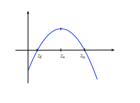
Figure 1: Shape of $F$.

(3) Assume that $s>1$. The derivative $F^{\prime}(z)=1-s{a}z^{s-1}$ has a unique zero at $z_{*}=(\frac{1}{s{a}})^{\frac{1}{s-1}}$ and

$$\begin{array}[]{ll}F(z_{*})=&\left(\frac{1}{s{a}}\right)^{\frac{1}{s-1}}-{a}\left(\frac{1}{s{a}}\right)^{\frac{s}{s-1}}-{b}>0,\\ \end{array}$$

by our hypothesis (19). Since $F(0)=-{b}<0$ and $F(z)\rightarrow-\infty$ as $z\rightarrow+\infty$ we see that the shape of $F$ is as in Fig.1. For $t\in\mathbb{N}$, let $Z(t)=(1+2|\hat{x}(t_{*})|^{2})^{\frac{1}{2}},$ where $t_{*}$ is defined as in (21), i.e., $t_{*}\in\mathrm{argmax}_{0\leq\tau\leq t}|\hat{x}(\tau)|$. For $t=0$ we must have $t_{*}=0$ and

$$\begin{array}[]{ll}Z(0)=(1+2|\hat{x}(0)|^{2})^{\frac{1}{2}}\leq 1+\sqrt{2}|\hat{x}(0)|={b}\leq(\frac{1}{s{a}})^{\frac{1}{s-1}}=z_{*}.\end{array}$$

This implies that $Z(0)\leq z_{\ell}.$ Assume that there exists $t\in\mathbb{N}$ such that $Z(t)\geq z_{u}$ and let $t_{0}$ be the first such $t$. Then ${t_{0}}_{*}=t_{0}\geq 1$ and for all $t<t_{0},$

$$\begin{array}[]{ll}(1+2|\hat{x}(t)|^{2})^{\frac{1}{2}}\leq z_{\ell}\leq z_{*},\end{array}$$

that is,

$$\begin{array}[]{ll}|\hat{x}(t)|\leq\big{(}\frac{{z_{*}}^{2}-1}{2}\big{)}^{\frac{1}{2}}.\end{array}$$

In particular,

$$\begin{array}[]{ll}|\hat{x}(t_{0}-1)|^{2}\leq\frac{{z_{\ell}}^{2}-1}{2}\leq\frac{{z_{*}}^{2}-1}{2}.\end{array}$$

On the other hand, $Z(t_{0})\geq z_{u}$ gives

$$\begin{array}[]{ll}|\hat{x}(t_{0})|^{2}\geq\frac{{z_{u}}^{2}-1}{2}\geq\frac{{z_{*}}^{2}-1}{2}.\end{array}$$

Thus we have

$$|\hat{x}(t_{0})|^{2}-|\hat{x}(t_{0}-1)|^{2}\geq\frac{{z_{*}}^{2}-{z_{\ell}}^{2}}{2}\geq\frac{1}{2}(z_{*}-z_{\ell})z_{*}.$$ (23)

By the intermediate value theorem, there is a $\xi\in[z_{\ell},z_{*}]$ such that $F(z_{*})=F^{\prime}(\xi)(z_{*}-z_{\ell}).$ Note that $F^{\prime}(\xi)=1-s{a}\xi^{s-1}\in[0,1]$, therefore,

$$\begin{array}[]{ll}z_{*}-z_{\ell}\geq F(z_{*}).\end{array}$$

We combine (23) to obtain

$$|\hat{x}(t_{0})|^{2}-|\hat{x}(t_{0}-1)|^{2}\geq\frac{1}{2}z_{*}F(z_{*}).$$ (24)

However, we have

$$|\hat{x}(t_{0})|-|\hat{x}(t_{0}-1)|\leq|\hat{x}(t_{0})-\hat{x}(t_{0}-1)|=h|\hat{v}(t_{0}-1)|\leq 2h\lambda|v(0)|_{\infty}\leq 2h\lambda|v(0)|.$$

Therefore,

$$\begin{array}[]{ll}|\hat{x}(t_{0})|^{2}-|\hat{x}(t_{0}-1)|^{2}&=\left(|\hat{x}(t_{0})|-|\hat{x}(t_{0}-1)|\right)^{2}+2\left(|\hat{x}(t_{0})|-|\hat{x}(t_{0}-1)|\right)|\hat{x}(t_{0}-1)|\\ &\leq 4h^{2}\lambda^{2}|v(0)|^{2}+4h\lambda|v(0)||\hat{x}(t_{0}-1)|\\ &\leq 4h^{2}\lambda^{2}|v(0)|^{2}+4h\lambda|v(0)|\left(\frac{{z_{*}}^{2}-1}{2}\right)^{\frac{1}{2}}.\end{array}$$

We combine this inequality with (24) to obtain

$$\begin{array}[]{ll}z_{*}F(z_{*})\leq 8h^{2}\lambda^{2}|v(0)|^{2}+8h\lambda|v(0)|\left(\frac{{z_{*}}^{2}-1}{2}\right)^{\frac{1}{2}}\leq 8h^{2}\lambda^{2}|v(0)|^{2}+4\sqrt{2}h\lambda|v(0)|z_{*},\end{array}$$

thus, we have

$$F(z_{*}) =\left(\frac{1}{{a}}\right)^{\frac{1}{s-1}}\left[\left(\frac{1}{s}\right)^{\frac{1}{s-1}}-\left(\frac{1}{s}\right)^{\frac{s}{s-1}}\right]-{b}$$

$$\leq 8h^{2}\lambda^{2}|v(0)|^{2}\left(s{a}\right)^{\frac{1}{s-1}}+4\sqrt{2}h\lambda|v(0)|$$

$$\leq\frac{8\lambda^{2}|v(0)|^{2}s^{\frac{1}{s-1}}}{N^{2}}{a}^{\frac{1}{s-1}}+\frac{4\sqrt{2}\lambda|v(0)|}{N},$$

where (10) is used. This contradicts to our hypothesis (19). So we conclude that, for all $T\in\mathbb{N}$, $Z(t)\leq z_{\ell}$ and then $|\hat{x}(t)|\leq\big{(}\frac{{z_{*}}^{2}-1}{2}\big{)}^{\frac{1}{2}},$ which is a uniform bound for $\hat{x}(t)$. Again we can proceed as in case (1) to complete the proof. ∎

IV Simulations

In this section, we present some numerical simulations to show the flocking behavior in a C-S model with alternating leaders. For these simulations, we choose a flock consisting of three agents, labeled by $\mathcal{V}=\{1,2,3\}$, and we take the parameters

$$h=0.2,\quad\mathrm{and}\quad\beta=\frac{1}{4}.$$

We consider the switching in three interaction topologies described by graphs

$$\mathcal{G}_{1}=\big{(}\mathcal{V},\{(1,2),(1,3)\}\big{)},\,\,\mathcal{G}_{2}=\big{(}\mathcal{V},\{(2,1),(2,3)\}\big{)},\,\,\mathcal{G}_{3}=\big{(}\mathcal{V},\{(3,1),(3,2)\}\big{)}.$$

This means that in $\mathcal{G}_{i}$, the agent $i$ acts as the leader and there are information flows from $i$ to the other two agents. We choose the switching signal $\sigma(t)$ as

$$\sigma(t)=(t,~{}\mod 3)+1,\qquad t\,\,\textrm{is the discrete time mark}.$$

In other words, the sequence of neighbor graphs is given by

$$\mathcal{G}_{1}\to\mathcal{G}_{2}\to\mathcal{G}_{3}\to\mathcal{G}_{1}\to\mathcal{G}_{2}\to\cdots,$$ (25)

and at each time step, there is a switching in the neighbor graphs; that is, the dwelling time for each active graph is $T_{d}=h=0.2$. For the initial state, we choose the initial position $x(0)\in(\mathbb{R}^{3})^{3}$ with nine coordinates randomly distributed in an interval of length 10; while the coordinates of initial velocities were randomly chosen from an interval of unit length. In Figure 2 we show the evolution of relative positions $\hat{x}_{i}=x_{i}-x_{3}$ and the evolution of the norm of total relative velocity $(|\hat{v}_{1}|^{2}+|\hat{v}_{2}|^{2})^{\frac{1}{2}}$. These simulations show the asymptotic (exponentially fast) flocking behavior of the C-S model with alternating leaders.

In Figure 3 (a), we also exhibit the evolution of velocities $v_{1}$, $v_{2}$, and $v_{3}$ under the switching signal $\sigma$. Here, we use different colors to denote different coordinates, and use different markers to describe different agents. Figure 3 (a) indicates that each coordinate of their velocities asymptotically attains an alignment, i.e., they exhibit a velocity consensus asymptotically. To compare the relaxation process of the flocking state under different switching topology, we did some simulations with different switching signal. We chose the similar signal with a sequence (25) but with a different dwelling time $T_{d}$ for each neighbor graph. Precisely, we take $T_{d}=1$ seconds, $T_{d}=3$ seconds and $T_{d}=7$ seconds for the simulations exhibited in Figure 3 (b), (c) and (d), respectively. We observe that in any case the velocities attain a near alignment after $t_{0}=9$ and keep like this. This means that the flocking state is robust about the alternating leaders. Moreover, we observe that the switching signal before the alignment influence the asymptotic value a lot. Since the leader in the first active interaction topology is agent 1, if the dwelling time is longer, the asymptotic velocity is more close to the initial value of the agent 1.

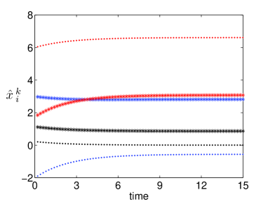
(a) The evolution of each coordinate of relative positions $\hat{x}^{k}_{i}=x^{k}_{i}-x^{k}_{3},\,\,i=1,2,\,k=1,2,3.$

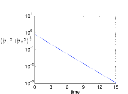
(b) The evolution of $(|\hat{v}_{1}|^{2}+|\hat{v}_{2}|^{2})^{\frac{1}{2}}$ for the relative velocities $\hat{v}_{i}=v_{i}-v_{3},\,\,i=1,2.$

Figure 2: The emergence of flocking in a 3-agent C-S model with alternating leaders

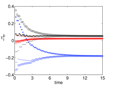
(a) $T_{d}=h=0.2$

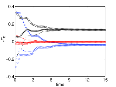
(b) $T_{d}=1$

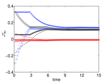
(c) $T_{d}=3$

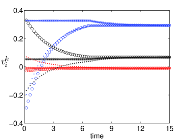
(d) $T_{d}=7$

Figure 3: The velocity alignment in a 3-agent C-S model with alternating leaders. The lines in blue, red and black indicate $x$, $y$ and $z$ coordinates, respectively. The lines marked by star, circle and dot indicate the agent 1, 2 and 3, respectively.

V Conclusion

We studied the Cucker-Smale flocking under the rooted leadership with alternating leaders. This dynamically changing interaction topology is motivated by the ubiquitous phenomena in our nature such as the alternating leaders in migratory birds on the long journey, the changing political leaders in human societies, etc. Our study showed that the flocking behavior can occur for such a dynamically changed leadership structure under some sufficient conditions on the initial configurations depending on the decay rate of communications and the size of flocking.

References

• [1] S. Ahn, H.-O. Bae, S.-Y. Ha, Y. Kim and H. Lim, Application of flocking mechanism to the modeling of stochastic volatility, Math. Models Methods Appl. Sci. 23 (2013) 1603-1628.
• [2] S. Ahn, H. Choi, S.-Y. Ha and H. Lee, On collision-avoiding initial configurations to Cucker-Smale type flocking models, Comm. Math. Sci. 10 (2012) 625-643.
• [3] S. Ahn and S.-Y. Ha, Stochastic flocking dynamics of the Cucker-Smale model with multiplicative white noises, J. Math. Phys. 51 (2010) 103301.
• [4] M. Cao, A. S. Morse and B. D. O. Anderson, Reaching a consensus in a dynamically changing environment: A graphic approach, SIAM J. Control Optim. 47 (2008) 575-600.
• [5] M. Cao, A. S. Morse and B. D. O. Anderson, Reaching a consensus in a dynamically changing environment: Vonvergence rates, meansurement delays, and asynchronous events, SIAM J. Control Optim. 47 (2008) 601-623.
• [6] J. A. Carrillo, M. Fornasier, J. Rosado and G. Toscani, Asymptotic flocking dynamics for the kinetic Cucker-Smale model, SIAM J. Math. Anal. 42 (2010) 218-236.
• [7] F. Cucker and J.-G. Dong: On the critical exponent for flocks under hierarchical leadership, Math. Models Methods Appl. Sci. 19 (2009) 1391-1404.
• [8] F. Cucker and J.-G. Dong, Avoiding collisions in flocks, IEEE Trans. Automatic Control 55 (2010) 1238-1243.
• [9] F. Cucker and C. Huepe, Flocking with informed agents, MathS in Action 1 (2008) 1-25.
• [10] F. Cucker and E. Mordecki, Flocking in noisy environments, J. Math. Pures Appl. 89 (2008) 278-296.
• [11] F. Cucker and S. Smale, Emergent behavior in flocks, IEEE Trans. Automat. Control 52 (2007) 852-862.
• [12] F. Cucker and S. Smale, On the mathematics of emergence, Japan. J. Math. 2, (2007) 197-227.
• [13] F. Cucker, S. Smale and D. Zhou, Modeling language evolution, Found. Comput. Math. 4 (2004) 315–343.
• [14] R. Diestel, Graph Theory, Graduate Texts in Mathematics. New York, U.S.A.: Springer-Verlag, 1997.
• [15] S.-Y. Ha, K. Kim and K. Lee, A mathematical model for multi-name Credit based on the community flocking, To appear in Quantitative Finance.
• [16] S.-Y. Ha, K. Lee and D. Levy, Emergence of time-asymptotic flocking in a stochastic Cucker-Smale system, Commun. Math. Sci. 7 (2009) 453-469.
• [17] S.-Y. Ha, Z. Li, M. Slemrod and X. Xue, Flocking behavior of the Cucker-smale model under rooted leadership in a large coupling limit, To appear in Quart. Appl. Math.
• [18] S.-Y. Ha and J.-G. Liu, A simple proof of Cucker-Smale flocking dynamics and mean field limit, Commun. Math. Sci. 7 (2009) 297-325.
• [19] S.-Y. Ha and E. Tadmor, From particle to kinetic and hydrodynamic description of flocking, Kinetic and Related Models 1 (2008) 415-435.
• [20] A. Jadbabaie, J. Lin and A. Morse, Coordination of groups of mobile autonomous agents using nearest neighbor rules, IEEE Trans. Autom. Control 48 (2003) 988-1001.
• [21] J. Kang, S.-Y. Ha, E. Jeong and K.-K. Kang, How do cultural classes emerge from assimilation and distinction? An extension of the Cucker-Smale flocking Model, To appear in J. Math. Sociology.
• [22] G. Latouche and V. Ramaswami, Introduction to Matrix Analytic Methods in Stochastic Modeling. PH Distributions, ASA SIAM, 1999.
• [23] N. E. Leonard, D. A. Paley, F. Lekien, R. Sepulchre, D. M. Fratantoni and R. E. Davis, Collective motion, sensor networks and ocean sampling, Proc. IEEE 95 (2007) 48-74.
• [24] Z. Li, S.-Y. Ha and X. Xue, Emergent phenomena in an ensemble of Cucker-Smale particles under joint rooted leadership, To appear in Math. Models Methods Appl. Sci.
• [25] Z. Li and X. Xue, Cucker-Smale flocking under rooted leadership with fixed and switching topologies, SIAM J. Appl. Math. 70 (2010) 3156-3174.
• [26] J. Park, H. Kim and S.-Y. Ha, Cucker-Smale flocking with inter-particle bonding forces, IEEE Tran. Automatic Control 55 (2010) 2617-2623.
• [27] L. Perea, G. Gómez and P. Elosegui, Extension of the Cucker-Smale control law to space flight formation, J. Guidance, Control and Dynamics 32 (2009) 526-536.
• [28] J. Shen, Cucker-Smale flocking under hierarchical leadership, SIAM J. Appl. Math. 68 (2007) 694-719.
• [29] J. Toner and Y. Tu, Flocks, herds, and Schools: A quantitative theory of flocking, Physical Review E. 58 (1998) 4828-4858.
• [30] T. Vicsek, A. Czirók, E. Ben-Jacob, I. Cohen and O. Schochet, Novel type of phase transition in a system of self-driven particles, Phys. Rev. Lett. 75 (1995) 1226-1229.
• [31] X. Xue and L. Guo, A kind of nonnegative matrices and its application on the stability of discrete dynamical systems, J. Math. Anal. Appl. 331 (2007) 1113-1121.
• [32] X. Xue and Z. Li, Asymptotic stability analysis of a kind of switched positive linear discrete systems, IEEE Trans. Autom. Control 55 (2010) 2198-2203.