Localized and complete resonance in plasmonic structures

Abstract

This paper studies a possible connection between the way the time averaged electromagnetic power dissipated into heat blows up and the anomalous localized resonance in plasmonic structures. We show that there is a setting in which the localized resonance takes place whenever the resonance does and moreover, the power is always bounded and might go to $0$. We also provide another setting in which the resonance is complete and the power goes to infinity whenever resonance occurs; as a consequence of this fact there is no localized resonance. This work is motivated from recent works on cloaking via anomalous localized resonance.

1 Introduction and statement of the main results

Negative index materials (NIMs) were first investigated theoretically by Veselago in [16] and were innovated by Nicorovici et al. [13] in the electrical impedance setting and by Pendry [14] in the electromagnetic setting. The existence of such materials was confirmed by Shelby, Smith, and Schultz in [15]. An interesting (and surprising) property on NIMs is the anomalous localized resonance discovered by Nicorovici et al. in [13] for core-shell plasmonic structures in two dimensions in which a circular shell has permitivity $-1+i\delta$ while the core and the matrix, the complement of the core-shell structure, have permitivity $1$. Here $\delta$ describes the loss of the material (more precisely, the loss of the negative index material part). A key figure of the phenomenon is the localized resonance of the field, i.e., the field blows up in some regions and remains bounded in some others as $\delta\to 0$. This is partially due to the change sign of the coefficient in the equation and therefore the ellipticity is lost as $\delta\to 0$; the loss of ellipticity is not sufficient to ensure such a property as discussed later in this paper. Following [7], the localized resonance is anomalous because the boundary of the resonant regions varies with the position of the source, and their boundary does not coincide with any discontinuity in moduli.

An attractive application related to the anomalous localized resonance is cloaking. This was recognized by Milton and Nicorovici in [7] and investigated in [1, 2, 3, 4, 5, 8] and the references therein. Let us discuss two results related to cloaking via anomalous localized resonance obtained so far for non radial core shell structures in [1, 5], in which the authors deal with the two dimensional quasistatic regime. In [1], the authors provide a necessary and sufficient condition on the source for which the time averaged electromagnetic power dissipated into heat blows up as the loss goes to zero using the spectral method. Their characterization is based on the detailed information on the spectral properties of a Neumann-Poincaré type operator. This information is difficult to come by in general. In [5], using the variational approach, the authors show that the power goes to infinity if the location of the source is in a finite range w.r.t. the shell for a class of sources. The core is not assumed to be radial but the matrix is in [5]. The boundedness of the fields in some regions for these structures is not discussed in [1, 5] except in the radial case showed in [1] (see also [7, 13]). It is of interest to understand if there is a possible connection between the power and the localized resonance in general.

In this paper, we present two settings in which there is no connection between the blow up of the power and the localized resonance. To this end, the following two problems are considered.

Problem 1: The behaviour of $u_{\delta}\in H^{1}(B_{R})$ ($R>1$) the unique solution to

$$\left\{\begin{array}[]{cl}\operatorname{div}(\varepsilon_{\delta}\nabla u_{\delta})=0&\mbox{ in }B_{R},\\[6.0pt] u_{\delta}=g&\mbox{ on }\partial B_{R},\end{array}\right.$$ (1.1)

where $g\in H^{1/2}(\partial B_{R})$ and the way the power, which will be defined in (1.6), explodes as $\delta\to 0_{+}$.

Here and in what follows $B_{r}$ denotes the ball centred at the origin of radius $r$ for $r>0$.

Problem 2: The behaviour of $u_{\delta}\in W^{1}(\mathbb{R}^{2})$ (see (1.16) for the notation) the unique solution converging to 0 as $|x|\to\infty$ to

$$\operatorname{div}(\varepsilon_{\delta}\nabla u_{\delta})=f\mbox{ in }\mathbb{R}^{2},$$ (1.2)

and the way the power, defined in (1.6), explodes. Here $f$ is in $L^{2}(\mathbb{R}^{2})$ with compact support in $\mathbb{R}^{2}\setminus B_{1}$ and satisfies the compatible condition

$$\int_{\mathbb{R}^{2}}f=0.$$ (1.3)

For $0\leq\delta<1$, $\varepsilon_{\delta}$ is defined by

$$\varepsilon_{\delta}:=\left\{\begin{array}[]{cl}(F^{-1})_{*}I&\mbox{ if }|x|>1\\[6.0pt] -1+i\delta&\mbox{ if }|x|<1,\end{array}\right.\quad\mbox{ for }d=2,\,3,$$ (1.4)

where $F:\mathbb{R}^{d}\setminus B_{1}\to\bar{B}_{1}$ is the Kelvin transform w.r.t. $\partial B_{1}$, i.e., $F(x)=x/|x|^{2}$.

Here and in what follows, we use the following standard notation

$$T_{*}a(y)=\frac{DT(x)a(x)DT^{T}(x)}{J(x)}\quad\mbox{ and }\quad T_{*}f(y)=\frac{f(x)}{J(x)}.$$ (1.5)

where $x=T^{-1}(y)$ and $J(x)=|\det DT(x)|$, for $f\in L^{2}(D_{1})$, $a\in[L^{\infty}(D_{1})]^{d\times d}$, $f\in L^{2}(D_{1})$, and $T$ a diffeomorphism from $D_{1}$ onto $D_{2}$.

It is easy to verify that, as noted in [9],

$$\varepsilon_{\delta}:=\left\{\begin{array}[]{cl}1&\mbox{ if }|x|>1\\[6.0pt] -1+i\delta&\mbox{ if }|x|<1\end{array}\right.\quad\mbox{ for }d=2.$$

The media considered in Problems 1 and 2 where $\varepsilon_{\delta}$ is given in (1.4) have the complementary property (see [9] for the definition and a discussion on various results related to these media in a general core shell structure). The setting studied in [5] also inherits this property since the matrix is radial while the setting in [1] is not in general. As seen later, this property is not enough to ensure a connection between the blow up of the power and the localized resonance.

In Problems 1 and 2, $\delta$ is the loss of the media (more precisely the loss of the negative index material in $B_{1}$) and the time averaged power dissipated into heat is given by (see, e.g., [1, 5])

$$E_{\delta}(u_{\delta})=\delta\int_{B_{1}}|\nabla u_{\delta}|^{2}\,dx.$$ (1.6)

From the definition of $u_{\delta}$, one can derive that

$$\int_{B_{1}}|\nabla u_{\delta}|^{2}\,dx\geq\left\{\begin{array}[]{cl}\displaystyle C_{1}\int_{B_{R}}\displaystyle|\nabla u_{\delta}|^{2}-C_{2}\|g\|_{H^{1/2}(\partial B_{R})}^{2}&\mbox{ in Problem 1},\\[6.0pt] \displaystyle C_{1}\int_{\mathbb{R}^{2}}|\nabla u_{\delta}|^{2}-C_{2}\|f\|_{L^{2}}^{2}&\mbox{ in Problem 2},\end{array}\right.$$

for some positive constants $C_{1}$, $C_{2}$ independent of $\delta$, $f$, and $g$.

The main results of the paper are Theorems 1 and 2 below. Concerning Problem 1, we have.

Theorem 1.

Let $d=2,3$, and $g\in H^{1/2}(\partial B_{R})$ and $u_{\delta}\in H^{1}(B_{R})$ be the unique solution to (1.1). Then

1. Case 1: $g$ is compatible to (1.1) (see Definition 1). Then $\big{(}\|u_{\delta}\|_{H^{1}(B_{R})}\big{)}$ remains bounded. Moreover, $u_{\delta}\to u_{0}$ weakly in $H^{1}(B_{R})$ as $\delta\to 0$ where $u_{0}\in H^{1}(B_{R})$ is the unique solution to

   $$\left\{\begin{array}[]{cl}\operatorname{div}(\varepsilon_{0}\nabla u_{0})=0&\mbox{ in }B_{R},\\[6.0pt] u_{0}=g&\mbox{ on }\partial B_{R}.\end{array}\right.$$ (1.7)

2. Case 2: $g$ is not compatible to (1.1). Then

   $$\lim_{\delta\to 0}\|u_{\delta}\|_{H^{1}(B_{R})}=+\infty;$$ (1.8)

   however,

   $$u_{\delta}\to v\mbox{ weakly in }H^{1}(B_{1/R}),$$ (1.9)

   where $v\in H^{1}(B_{1/R})$ is the unique solution to

   $$\left\{\begin{array}[]{cl}\Delta v=0&\mbox{in }B_{1/R},\\[6.0pt] v(x)=h(x):=g(x/|x|^{2})&\mbox{on }\partial B_{1/R}.\end{array}\right.$$ (1.10)

   Moreover, for all $g\in H^{1/2}(\partial B_{R})$,

   $$\limsup_{\delta\to 0}\delta\int_{B_{R}}|\nabla u_{\delta}|^{2}dx<+\infty,$$ (1.11)

   and for any $0<\alpha<1/2$, there exists $g\in H^{1/2}(\partial B_{R})$ such that

   $$0<\liminf_{\delta\to 0}\delta^{2\alpha}\int_{B_{R}}|\nabla u_{\delta}|^{2}dx\leq\limsup_{\delta\to 0}\delta^{2\alpha}\int_{B_{R}}|\nabla u_{\delta}|^{2}dx<+\infty.$$ (1.12)

Remark 1.

Concerning (1.1), whenever resonance takes place , it is localized in the sense that the field blows up in some region and remains bounded in some others; moreover, the power remains bounded and might converge to 0 as $\delta\to 0$ .

In the statement of Theorem 1, we use the following definition.

Definition 1.

Let $g\in H^{1/2}(\partial B_{R})$. Then $g$ is said to be compatible to (1.1) if and only if there exists a solution $w\in H^{1}(B_{1}\setminus B_{1/R})$ to the Cauchy problem

$$\left\{\begin{array}[]{cl}\Delta w=0&\mbox{in }B_{1}\setminus B_{1/R},\\[6.0pt] w=v\mbox{ and }\partial_{\nu}w=\partial_{\nu}v&\mbox{on }\partial B_{1/R},\end{array}\right.$$ (1.13)

where $v$ is the function defined in (1.10). Otherwise, $g$ is not compatible.

Remark 2.

Figure 1 in Section 4 provides a numerical simulation illustrating Theorem 1.

Concerning Problem 2, we have.

Theorem 2.

Let $f\in L^{2}(\mathbb{R}^{2})$ be such that $\operatorname{supp}f\subset\subset\mathbb{R}^{d}\setminus B_{1}$ and (1.3) holds and let $u_{\delta}\in W^{1}(\mathbb{R}^{2})$ be the unique solution converging to 0 as $|x|\to\infty$ to (1.2). Then

1. Case 1: $f$ is compatible to (1.2) (see Definition 2). Then

   $$u_{\delta}=U:=\left\{\begin{array}[]{cl}w\circ F-w(0)&\mbox{ in }\mathbb{R}^{2}\setminus B_{1},\\[6.0pt] -w(0)&\mbox{ in }B_{1}.\end{array}\right.$$ (1.14)

   Here $w$ will be defined in (1.17).

2. Case 2: $f$ is not compatible to (1.2). Then

   $$0<\liminf_{\delta\to 0}\delta^{2}\int_{O}|\nabla u_{\delta}|^{2}\,dx\leq\limsup_{\delta\to 0}\delta^{2}\int_{O}|\nabla u_{\delta}|^{2}\,dx<+\infty,$$ (1.15)

   for any open subset $O$ of $\mathbb{R}^{2}$.

Remark 3.

Inequalities (1.15) implies that the field blows up in any open subset of $\mathbb{R}^{2}$ at the same rate .

Remark 4.

Theorem 2 also holds for $d=3$ (see the proof of Theorem 2 and Remark 6, which is about representations in $B_{1}$). However, in this case, the existence of $u_{\delta}$ belongs to some Sobolev spaces with weight since $(F^{-1})_{*}I$ is not bounded from below by a positive constant at infinity due to the fact $d=3$. We do not treat this case in this paper to keep the presentation simple.

For $U$ a smooth open region of $\mathbb{R}^{2}$ with a bounded complement (this includes $U=\mathbb{R}^{2}$), we use the following standard notation:

$$W^{1}(U)=\left\{u\in L^{2}_{{}_{loc}}(U);\;\nabla u\in\big{[}L^{2}(U)\big{]}^{2}\mbox{ and }\frac{u}{|x|\log(2+|x|)}\in L^{2}(U)\right\}.$$ (1.16)

Part of Theorem 2 was considered in [5]. More precisely, in [5], the authors showed that $E_{\delta}(u_{\delta})\to\infty$ for $f$ with $\operatorname{supp}f\subset\partial B_{r}$ for $r>1$ . In this paper, we make one step further. We show that when resonance occurs, it is complete in the sense that (1.15) holds; there is no localized resonance here. Otherwise, the field remains bounded. In fact it is independent of $\delta$ by (1.14).

In the statement of Theorem 2, we use the following definition.

Definition 2.

Let $f\in L^{2}(\mathbb{R}^{2})$ with $\operatorname{supp}f\subset\mathbb{R}^{2}\setminus B_{1}$. Then $f$ is said to be compatible to (1.2) if and only if there exists a solution $w\in H^{1}(B_{1})$ to the Cauchy problem

$$\left\{\begin{array}[]{cl}\Delta w=F_{*}f&\mbox{ in }B_{1},\\[6.0pt] \partial_{\nu}w=w=0&\mbox{ on }\partial B_{1}.\end{array}\right.$$ (1.17)

Otherwise, $f$ is not compatible.

Remark 5.

Figure 2 in Section 4 provides a numerical simulation illustrating Theorem 2.

From Theorems 1 and 2, we conclude that in the settings considered in this paper, there is no connection between the unboundedness of the power and the localized resonance. Though the settings in Problems 1 and 2 are very similar, the essence of the resonance are very different. A connection between these phenomena would be linked not only to the location of the source but also to the geometry of the problem, i.e., the definition of $\varepsilon_{\delta}$. Using the concept of (reflecting) complementary media introduced in [9], one can extend the results this paper in a more general setting.

The definitions of compatibility conditions have roots from [9]. The analysis for the compatible cases is inspired from there. The analysis in the incompatible case is guided from the compatible one. One of the main observations in this paper is the localized resonant phenomena in (1.9) (one has localized resonance by (1.8)). The localized resonance is also discussed in the context of superlensing and cloaking using complementary media in [10, 11] where the removing of localized singularity technique was introduced by the first author to deal with localized resonance in non radial settings. In recent work [12], the first author introduces the concept of doubly complementary media for a general shell-core structure and shows that cloaking via anomalous localized resonance takes place if and only if the power blows up. To this end, he introduces and develops the technique of separation of variables for a general structure.

The paper is organized as follows. In Sections 2 and 3, we prove Theorems 1 and 2 respectively. In Section 4, we provide numerical simulations illustrating these results.

2 Proof of Theorem 1

2.1 Preliminaries

In this section, we present two elementary lemmas which are very useful for the proof of Theorem 1. The first one (Lemma 1) is on the change of variables for the Kelvin transform. Lemma 1 is a special case of [9, Lemma 4] which deals with general reflections.

Lemma 1.

Let $d=2,\,3$, $0<R_{1}<R_{2}<R_{3}$ with $R_{3}=R_{2}^{2}/R_{1}$, $f\in L^{2}(B_{R_{2}}\setminus B_{R_{1}})$, $a\in[L^{\infty}(B_{R_{2}\setminus R_{1}})]^{d\times d}$ be a uniformly elliptic matrix - valued function, and $K:B_{R_{2}}\setminus\bar{B}_{R_{1}}\to B_{R_{3}}\setminus\bar{B}_{R_{2}}$ be the Kelvin transform w.r.t $\partial B_{R_{2}}$, i.e.,

$$K(x)=R_{2}^{2}x/|x|^{2}.$$

For $v\in H^{1}(B_{R_{2}}\setminus B_{R_{1}})$, define $w=v\circ K^{-1}$. Then

$$\operatorname{div}(a\nabla v)=f\mbox{ in }B_{R_{2}}\setminus B_{R_{1}}$$

if and only if

$$\operatorname{div}(K_{*}a\nabla w)=K_{*}f\mbox{ in }B_{R_{3}}\setminus B_{R_{2}}.$$

Moreover,

$$w=v\quad\mbox{ and }\quad K_{*}a\nabla w\cdot\nu=-a\nabla v\cdot\nu\mbox{ on }\partial B_{R_{2}}.$$

The second lemma is on an estimate related to solutions to (1.1).

Lemma 2.

Let $d=2,\,3$, $f\in H^{-1}(B_{R})$, and let $U_{\delta}\in H^{1}_{0}(B_{R})$ be the unique solution to

$$\operatorname{div}(\varepsilon_{\delta}\nabla U_{\delta})=f\mbox{ in }B_{R}.$$

We have

$$\|U_{\delta}\|_{H^{1}(B_{R})}\leq\frac{C}{\delta}\|f\|_{H^{-1}}$$

for some positive constant $C$ independent of $f$ and $\delta$.

Proof. Lemma 2 follows from Lax-Milgram’s theorem. The details are left to the reader. $\Box$

2.2 Proof of Theorem 1

The proof is divided into 6 steps.

Step 1: We prove that if there exists a solution $u\in H^{1}(B_{R})$ to

$$\left\{\begin{array}[]{cl}\operatorname{div}(\varepsilon_{0}\nabla u)=0&\mbox{ in }B_{R},\\[6.0pt] u=g&\mbox{ on }\partial B_{R},\end{array}\right.$$ (2.1)

then $g$ is compatible. Moreover, the solution to (2.1) is unique in $H^{1}(B_{R})$.

In fact, define $V$ in $B_{1}\setminus B_{1/R}$ by

$$V=u\circ F^{-1}.$$

We have, by Lemma 1,

$$V=u\Big{|}_{\rm ext}\mbox{ and }\partial_{r}V=\partial_{r}u\Big{|}_{\rm ext}\mbox{ on }\partial B_{1}.$$

Set

$$W=u-V\mbox{ in }B_{1}\setminus B_{1/R}.$$

By Lemma 1, $W\in H^{1}(B_{1}\setminus B_{1/R})$ is a solution to the Cauchy problem

$$\left\{\begin{array}[]{cl}\Delta W=0&\mbox{ in }B_{1}\setminus B_{1/R},\\[6.0pt] \partial_{\nu}W=W=0&\mbox{ on }\partial B_{1}.\end{array}\right.$$

By the unique continuation principle, $W=0$. This implies

$$u=V=h\mbox{ on }\partial B_{1/R}.$$

Therefore, $u=v$ in $B_{1/R}$ where $v$ is defined in (1.10). It follows that $u$ satisfies (1.13) and $g$ is compatible. The uniqueness in $H^{1}(B_{R})$ of (2.1) is also clear from the analysis.

Step 2: We prove that if $g$ is compatible then $u_{\delta}\to u$ weakly in $H^{1}(B_{R})$ where

$$u=\left\{\begin{array}[]{cl}v&\mbox{ in }B_{1/R},\\[6.0pt] w&\mbox{ in }B_{1}\setminus B_{1/R},\\[6.0pt] w\circ F&\mbox{ in }B_{R}\setminus B_{1},\end{array}\right.$$

where $w$ is given in (1.13).

It is clear that $u\in H^{1}(B_{R})$ is a solution to (2.1). The uniqueness of $u$ follows from Step 1. Define

$$U_{\delta}=u_{\delta}-u\quad\mbox{ in }B_{R}.$$

Then $U_{\delta}\in H^{1}_{0}(B_{R})$ is the unique solution to

$$\operatorname{div}(\varepsilon_{\delta}\nabla U_{\delta})=\operatorname{div}\big{(}(\varepsilon_{0}-\varepsilon_{\delta})\nabla u\big{)}\mbox{ in }B_{R}.$$

This implies, by Lemma 2,

$$\|U_{\delta}\|_{H^{1}(B_{R})}\leq C\|\nabla u\|_{L^{2}(B_{R})}.$$

Since $u_{\delta}=U_{\delta}+u$, $(u_{\delta})$ is bounded in $H^{1}(B_{R})$. W.l.o.g. one may assume that $u_{\delta}$ converges weakly in $H^{1}(B_{R})$ to a solution to (2.1). Since (2.1) is uniquely solvable in $H^{1}(B_{R})$, the conclusion follows.

Step 3: We prove that if $\liminf_{\delta\to 0}\|\nabla u_{\delta}\|_{L^{2}(\mathbb{R}^{2})}<+\infty$ then $g$ is compatible.

Since $\liminf_{\delta\to 0}\|\nabla u_{\delta}\|_{L^{2}(\mathbb{R}^{2})}<+\infty$, there exists a solution $u\in H^{1}(B_{R})$ to (2.1). The conclusion now is a consequence of Step 1.

After Steps 1, 2, and 3, the first statement of Theorem 1 and (1.8) are established. We next prove (1.9), (1.11), and (1.12). We will only consider the two dimensional case. The proof in three dimensions follows similarly (see Remark 6). In what follows, we assume that $d=2$.

Step 4: Proof of (1.9).

Set

$$v_{\delta}=u_{\delta}\circ F^{-1}\mbox{ in }B_{1}\setminus B_{1/R}.$$

Then $v_{\delta}\in H^{1}(B_{1}\setminus B_{1/R})$ and

$$\Delta v_{\delta}=0\mbox{ in }B_{1}\setminus B_{1/R}.$$

One can represent $v_{\delta}$ as follows

$$v_{\delta}=a_{0}+b_{0}\log r+\sum_{n=1}^{\infty}\sum_{\pm}(a_{n,\pm}r^{n}+b_{n,\pm}r^{-n})e^{\pm in\theta}\mbox{ in }B_{1}\setminus B_{1/R},$$ (2.2)

for $a_{0},\,b_{0},a_{n,\pm},b_{n,\pm}\in\mathbb{C}$ ($n\geq 1$). Similarly, one can represent $u_{\delta}$ by

$$u_{\delta}=c_{0}+\sum_{n=1}^{\infty}\sum_{\pm}c_{n,\pm}r^{n}e^{\pm in\theta}\mbox{ in }B_{1},$$ (2.3)

for $c_{0},\,c_{n,\pm}\in\mathbb{C}$ ($n\geq 1$). Using the transmission conditions on $\partial B_{1}$, we have

$$v_{\delta}=u_{\delta}\Big{|}_{\rm int}\quad\mbox{ and }\quad\partial_{\nu}v_{\delta}=(1-i\delta)\partial_{\nu}u_{\delta}\Big{|}_{\rm int}\quad\mbox{ on }\partial B_{1}.$$ (2.4)

A combination of (2.2), (2.3), and (2.4) yields

$$\left\{\begin{array}[]{c}a_{n,\pm}+b_{n,\pm}=c_{n,\pm}\\[6.0pt] a_{n,\pm}-b_{n,\pm}=(1-i\delta)c_{n,\pm},\end{array}\right.\quad\mbox{ for }n\geq 1,$$

and

$$\left\{\begin{array}[]{c}a_{0}=c_{0}\\[6.0pt] b_{0}=0.\end{array}\right.$$ (2.5)

This implies

$$\left\{\begin{array}[]{l}\displaystyle a_{n,\pm}=(2-i\delta)c_{n,\pm}/2\\[6.0pt] \displaystyle b_{n,\pm}=i\delta c_{n,\pm}/2\end{array}\right.\mbox{ for }n\geq 1.\quad$$ (2.6)

From the definition of $v_{\delta}$, it is clear that

$$v_{\delta}=h=h_{0}+\sum_{n=1}^{\infty}\sum_{\pm}h_{n,\pm}e^{\pm in\theta}\mbox{ on }\partial B_{1/R},$$ (2.7)

for some $h_{0},\,h_{n,\pm}\in\mathbb{C}$ ($n\geq 1$). Since $v_{\delta}=h$ on $\partial B_{1/R}$, it follows from (2.2), (2.5), (2.6), and (2.7) that

$$\frac{1}{2}\left[(2-i\delta)R^{-n}+i\delta R^{n})\right]c_{n,\pm}=h_{n,\pm}\mbox{ for }n\geq 1$$ (2.8)

and

$$c_{0}=h_{0}.$$ (2.9)

We claim that

$$u_{\delta}-v_{\delta}\to 0\mbox{ weakly in }H^{1/2}(\partial B_{1/R}).$$ (2.10)

In fact, by (2.5) and (2.6), we have

$$u_{\delta}-v_{\delta}=\sum_{n=1}^{\infty}\sum_{\pm}\frac{1}{2}i\delta c_{n,\pm}(R^{-n}-R^{n})e^{\pm in\theta}\quad\mbox{ on }\partial B_{1/R}.$$ (2.11)

We derive from (2.8) and (2.11) that

$$u_{\delta}-v_{\delta}=\sum_{n=1}^{\infty}\sum_{\pm}\frac{i\delta(R^{-n}-R^{n})}{\big{[}2R^{-n}-i\delta(R^{-n}-R^{n})\big{]}}h_{n,\pm}e^{\pm in\theta}\quad\mbox{ on }\partial B_{1/R}.$$ (2.12)

Claim (2.10) follows since

$$\lim_{\delta\to 0}\frac{i\delta(R^{-n}-R^{n})}{\big{[}2R^{-n}-i\delta(R^{-n}-R^{n})\big{]}}=0\mbox{ for all }n\geq 1$$

and

$$\left|\frac{i\delta(R^{-n}-R^{n})}{\big{[}2R^{-n}-i\delta(R^{-n}-R^{n})\big{]}}\right|\leq 1\mbox{ for all }n\geq 1.$$

The conclusion of Step 4 is now a consequence of Claim (2.10) and the fact that $\Delta(u_{\delta}-v)=0$ in $B_{1/R}$.

Step 5: Proof of (1.11):

Since $\Delta u_{\delta}=0$ in $B_{R}\setminus\partial B_{1}$ and $u_{\delta}=g$ on $\partial B_{R}$, it suffices to prove that

$$\limsup_{\delta\to 0}\delta\|u_{\delta}\|_{H^{1/2}(\partial B_{1})}^{2}\leq C\|h\|_{H^{1/2}(\partial B_{1/R})}^{2}.$$

In this proof, $C$ denotes a positive constant independent of $\delta$ and $g$. From (2.3), (2.8), and (2.9), we have

$$C\|u_{\delta}\|_{H^{1/2}(\partial B_{1})}^{2}\leq|h_{0}|^{2}+\sum_{n=1}^{\infty}\sum_{\pm}\frac{n|h_{n}|^{2}}{4R^{-2n}+\delta^{2}(R^{n}-R^{-n})^{2}}.$$

We derive that

$$C\|u_{\delta}\|_{H^{1/2}(\partial B_{1})}^{2}\leq\sup_{n\geq 0}\frac{1}{4R^{-2n}+\delta^{2}(R^{n}-R^{-n})^{2}}\Big{(}|h_{0}|^{2}+\sum_{n=1}^{\infty}\sum_{\pm}n|h_{n,\pm}|^{2}\Big{)}.$$ (2.13)

Since $R>1$, it follows that

$$R^{-2n}+\delta^{2}(R^{n}-R^{-n})^{2}\geq C(R^{-2n}+\delta^{2}R^{2n})\geq 2C\delta\quad\forall\,n\geq 1.$$ (2.14)

A combination of (2.13) and (2.14) yields

$$C\delta\|u_{\delta}\|_{H^{1/2}(\partial B_{1})}^{2}\leq\|h\|_{H^{1/2}(\partial B_{1/R})}^{2};$$

hence (1.11) follows.

Step 6: Proof of (1.12).

Since $\Delta u_{\delta}=0$ in $B_{R}\setminus\partial B_{1}$ and $u_{\delta}=g$ on $\partial B_{R}$, it suffices to find $h\in H^{1/2}(\partial B_{1/R})$ such that

$$0<\liminf_{\delta\to 0}\delta^{2\alpha}\|u_{\delta}\|_{H^{1/2}(\partial B_{1})}^{2}\leq\limsup_{\delta\to 0}\delta^{2\alpha}\|u_{\delta}\|_{H^{1/2}(\partial B_{1})}^{2}<+\infty.$$ (2.15)

Recall that $h(x)=g(x/|x|^{2})$. Let $n_{\delta}=[\frac{1}{2}|\ln\delta/\ln R|]$ be the smallest integer that is greater than or equal to $\frac{1}{2}|\ln\delta/\ln R|$ ($R^{-2n_{\delta}}\sim\delta$). We have

$$\|u_{\delta}\|_{H^{1/2}(\partial B_{1})}^{2}\sim |h_{0}|^{2}+\sum_{n=1}^{\infty}\sum_{\pm}\frac{n|h_{n,\pm}|^{2}}{4R^{-2n}+\delta^{2}(R^{n}-R^{-n})^{2}}$$

$$\sim |h_{0}|^{2}+\sum_{n=1}^{n_{\delta}}\sum_{\pm}\frac{n|h_{n,\pm}|^{2}}{R^{-2n}}+\sum_{n=n_{\delta}+1}^{\infty}\sum_{\pm}\frac{n|h_{n,\pm}|^{2}}{\delta^{2}R^{2n}}.$$

Set

$$0<\gamma=1-2\alpha<1$$

and choose

$$h_{0}=0\quad\mbox{ and }\quad h_{n,\pm}=\frac{R^{-n\gamma}}{\sqrt{n}}\mbox{ for }n\geq 1.$$

It follows that, since $\gamma<1$ and $R>1$,

$$|h_{0}|^{2}+\sum_{n=1}^{n_{\delta}}\sum_{\pm}\frac{n|h_{n,\pm}|^{2}}{R^{-2n}}=2\sum_{n=1}^{n_{\delta}}R^{2n(1-\gamma)}\sim R^{2(1-\gamma)n_{\delta}}\sim\delta^{-2\alpha}$$ (2.16)

and, since $\gamma+1>0$ and $R>1$,

$$\sum_{n=n_{\delta}+1}^{\infty}\sum_{\pm}\frac{n|h_{n,\pm}|^{2}}{\delta^{2}R^{2n}}=\frac{2}{\delta^{2}}\sum_{n=n_{\delta}+1}^{\infty}R^{-2n(\gamma+1)}\sim\frac{1}{\delta^{2}}R^{-2(\gamma+1)n_{\delta}}\sim\delta^{-2\alpha}.$$ (2.17)

A combination of (2.16) and (2.17) yields (2.15).

It is clear that, since $\gamma>0$ and $R>1$,

$$\|h\|_{H^{1/2}(\partial B_{1/R})}^{2}\sim\sum_{n=1}^{\infty}\sum_{\pm}n|h_{n,\pm}|^{2}=2\sum_{n=1}^{\infty}R^{-2n\gamma}<+\infty.$$

The proof is complete. $\Box$

Remark 6.

We only prove (1.9), (1.11), and (1.12) for the two dimensions. The proof in the three dimensions follows similarly. In fact, in this case, $v_{\delta}$, $u_{\delta}$, and $h_{\delta}$ can be represented by

$$\left\{\begin{array}[]{cl}\displaystyle v_{\delta}(x)=\sum_{n=0}^{\infty}\sum_{k=-n}^{n}(a_{n}^{k}r^{n}+b_{n}^{k}r^{-n})Y^{k}_{n}(x/|x|)&\mbox{ in }B_{1}\setminus B_{1/R},\\[6.0pt] \displaystyle u_{\delta}(x)=\sum_{n=0}^{\infty}\sum_{k=-n}^{n}c_{n}^{k}r^{n}Y^{k}_{n}(x/|x|)&\mbox{ in }B_{1},\\[6.0pt] \displaystyle h(x)=\sum_{n=0}^{\infty}\sum_{k=-n}^{n}h_{n}^{k}Y^{k}_{n}(x/|x|)&\mbox{ on }\partial B_{1/R}.\end{array}\right.$$

The rest of the proof is almost unchanged.

3 Proof of Theorem 2

Step 1: We show that if there exists a solution $u\in W^{1}(\mathbb{R}^{2})$ to

$$\operatorname{div}(\varepsilon_{0}\nabla u)=f\mbox{ in }\mathbb{R}^{2},$$

then $f$ is compatible. This step is not necessary for the proof; however, it gives the motivation for the definition of the compatibility condition and it guides the proof.

Define $v$ in $B_{1}$ by

$$v=u\circ F^{-1}.$$

We have, by a change of variables,

$$\int_{B_{1}\setminus B_{r}}|\nabla v|^{2}dx=\int_{B_{r^{-1}}\setminus B_{1}}|\nabla u|^{2}dx.$$ (3.1)

Since $v$ is bounded in a neighborhood of the origin, it follows that $v\in H^{1}(B_{1})$ and $\Delta v=F_{*}f$ in $B_{1}$ by Lemma 1. We have, by Lemma 1 again,

$$v=u\Big{|}_{\rm ext}\mbox{ and }\partial_{r}v=-\partial_{r}u\Big{|}_{\rm ext}\mbox{ on }\partial B_{1}.$$

It follows that

$$v=u\Big{|}_{\rm int}\mbox{ and }\partial_{r}v=\partial_{r}u\Big{|}_{\rm int}\mbox{ on }\partial B_{1}.$$ (3.2)

Set

$$w=v-u\mbox{ in }B_{1}.$$

Then $w\in H^{1}(B_{1})$ is a solution to the Cauchy problem

$$\left\{\begin{array}[]{cl}\Delta w=F_{*}f&\mbox{ in }B_{1},\\[6.0pt] \partial_{\nu}w=w=0&\mbox{ on }\partial B_{1}\end{array}\right.$$

by (3.2). Therefore $f$ is compatible.

Step 2: Proof of statement 1).

It is clear that $U\in W^{1}(\mathbb{R}^{2})$ is a solution converging to 0 as $|x|\to\infty$ to (1.2). Statement 1) now follows from the uniqueness of such a solution.

Step 3: Proof of statement 2).

From (1.2) and (1.5), we have

$$\int_{B_{1}}F_{*}f=0.$$

Let $w\in H^{1}(B_{1})$ with $\displaystyle\int_{B_{1}}w=0$ be the unique solution to

$$\left\{\begin{array}[]{cl}\Delta w=F_{*}f&\mbox{ in }B_{1},\\[6.0pt] \partial_{\nu}w=0&\mbox{ on }\partial B_{1}.\end{array}\right.$$ (3.3)

Define

$$U_{\delta}=\left\{\begin{array}[]{cl}u_{\delta}&\mbox{in }B_{1},\\[6.0pt] u_{\delta}-w\circ F&\mbox{in }\mathbb{R}^{2}\setminus B_{1}.\end{array}\right.$$ (3.4)

Similar to (3.1), we have $U_{\delta}\in W^{1}(\mathbb{R}^{2}\setminus\partial B_{1})$. It is clear that

$$\Delta U_{\delta}=0\mbox{ in }\mathbb{R}^{2}\setminus\partial B_{1}.$$

Hence, one may represent $U_{\delta}$ as

$$U_{\delta}=\left\{\begin{array}[]{cl}\displaystyle a_{0}+\sum_{n=1}^{\infty}\sum_{\pm}a_{n,\pm}r^{n}e^{\pm in\theta}&\mbox{in }B_{1},\\[6.0pt] \displaystyle b_{0}+\sum_{n=1}^{\infty}\sum_{\pm}b_{n,\pm}r^{-n}e^{\pm in\theta}&\mbox{in }\mathbb{R}^{2}\setminus B_{1},\end{array}\right.$$ (3.5)

for $a_{0},b_{0},a_{n,\pm},b_{n,\pm}\in\mathbb{C}$ ($n\geq 1$). Assume that, on $\partial B_{1}$,

$$w=w_{0}+\sum_{n=1}^{\infty}\sum_{\pm}w_{n,\pm}e^{\pm in\theta},$$ (3.6)

for $w_{0},w_{n,\pm}\in\mathbb{C}$ ($n\geq 1$). From (3.4), we have

$$\left\{\begin{array}[]{c}U_{\delta}\Big{|}_{\rm ext}-U_{\delta}\Big{|}_{\rm int}=-w,\\[6.0pt] \partial_{\nu}U_{\delta}\Big{|}_{\rm ext}-(-1+i\delta)\partial_{\nu}U_{\delta}\Big{|}_{int}=0.\end{array}\right.$$ (3.7)

This implies

$$a_{n,\pm}=b_{n,\pm}+w_{n,\pm}\quad\mbox{ and }\quad(1-i\delta)a_{n,\pm}=b_{n,\pm},\quad\,\forall\,n\geq 1.$$ (3.8)

It follows that

$$a_{n,\pm}=\frac{w_{n,\pm}}{i\delta}\quad\mbox{ and }\quad b_{n,\pm}=\frac{(1-i\delta)w_{n,\pm}}{i\delta},\quad\,\forall\,n\geq 1.$$ (3.9)

for all $n\geq 1$. Noting that either $w_{n,+}\not=0$ or $w_{n,-}\not=0$ for some $n\geq 1$ since $f$ is not compatible, we obtain (1.15).

The proof of Theorem 2 is complete. $\Box$

4 Numerical illustrations

In this section we present some numerical results to illustrate Theorems 1 and 2. Figure 1 corresponds to Theorem 1 and presents a simulation on the localized resonance in which $R=3$ and $g=\sum_{n=1}^{\infty}\frac{1}{n^{2}}e^{in\theta}$. Figure 2 corresponds to Theorem 2 and presents a simulation on the complete resonance in which $f=\Delta(\phi g)\chi_{\mathbb{R}^{2}\setminus B_{1}}$ where $\chi$ denotes the characteristic function, $g=\sum_{n=1}^{\infty}\frac{r^{n}}{6^{n}}e^{in\theta}$ and $\phi\in C^{2}(\mathbb{R}^{2})$ is the radially symmetric function such that $\phi=1$ in $B_{2}$ and $\phi=0$ in $\mathbb{R}^{2}\setminus B_{3}$ . In both simulations, $g$ is approximated by its first hundred terms.

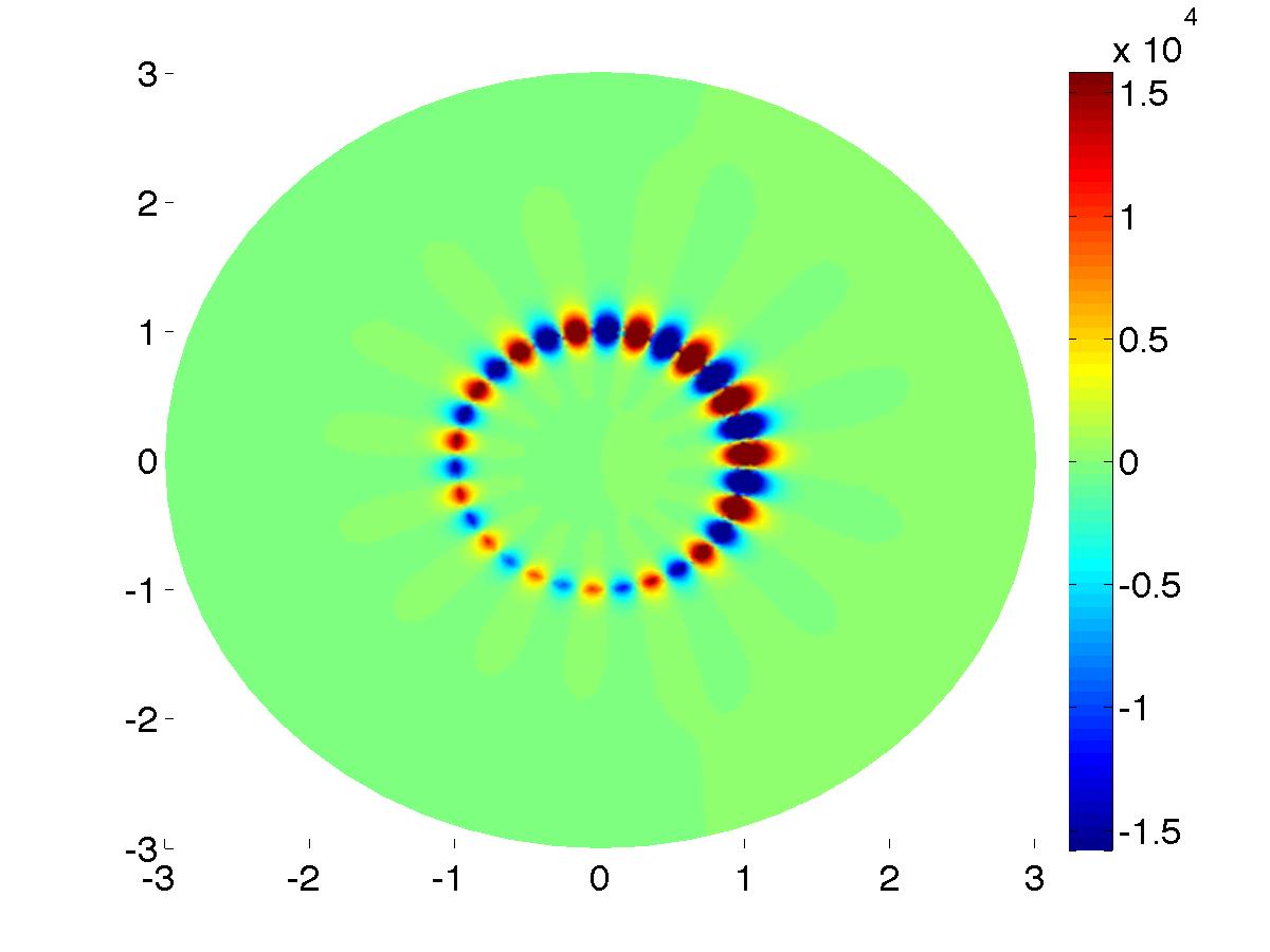
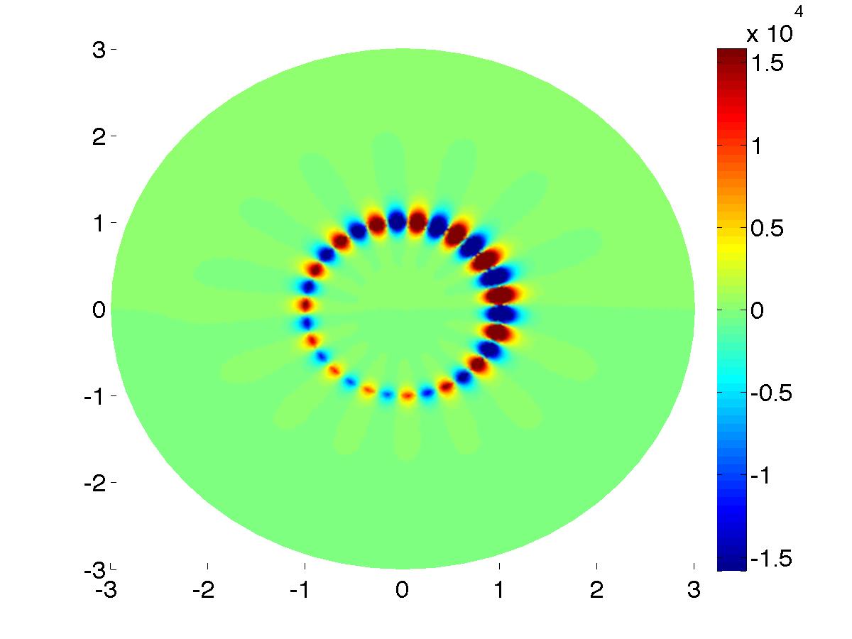
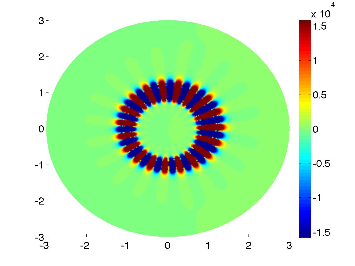
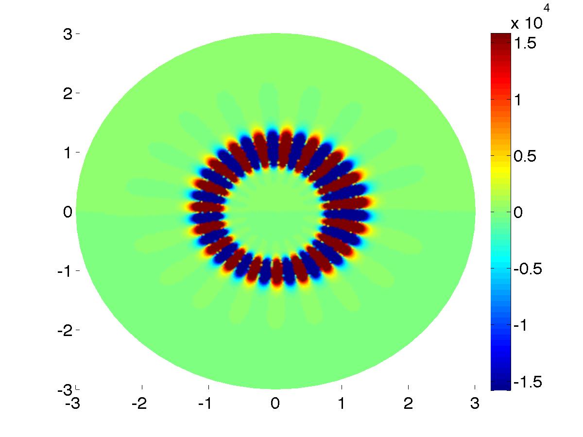
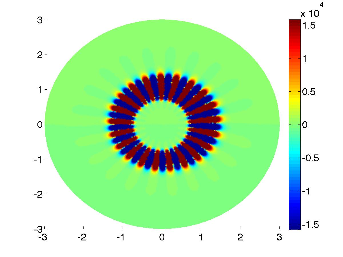
Figure 1: The graphs of $u_{\delta}$ when $\delta=10^{-14},10^{-18}$ and $10^{-20}$ from the $1^{\rm st}$ to the $3^{\rm rd}$ row. Left: the real part of $u_{\delta}$; Right: the imaginary part of $u_{\delta}.$

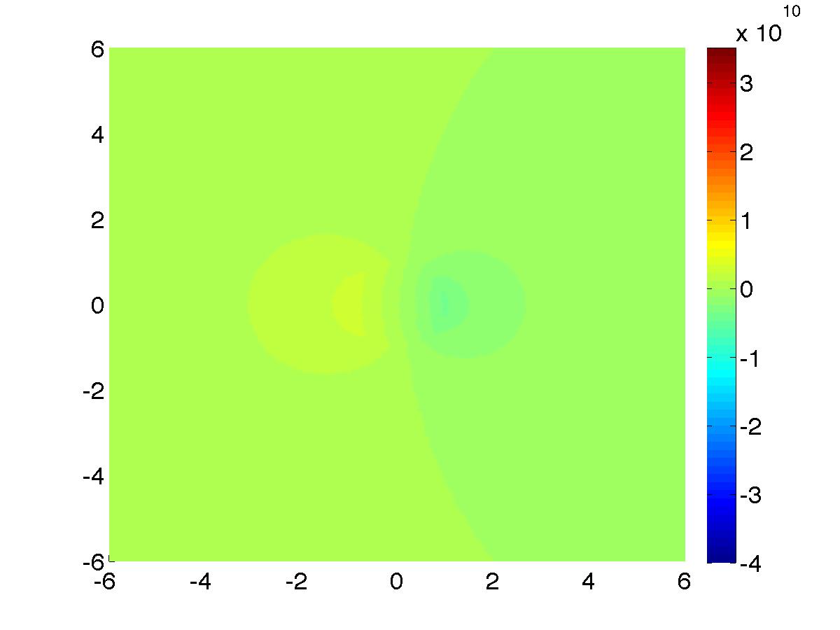
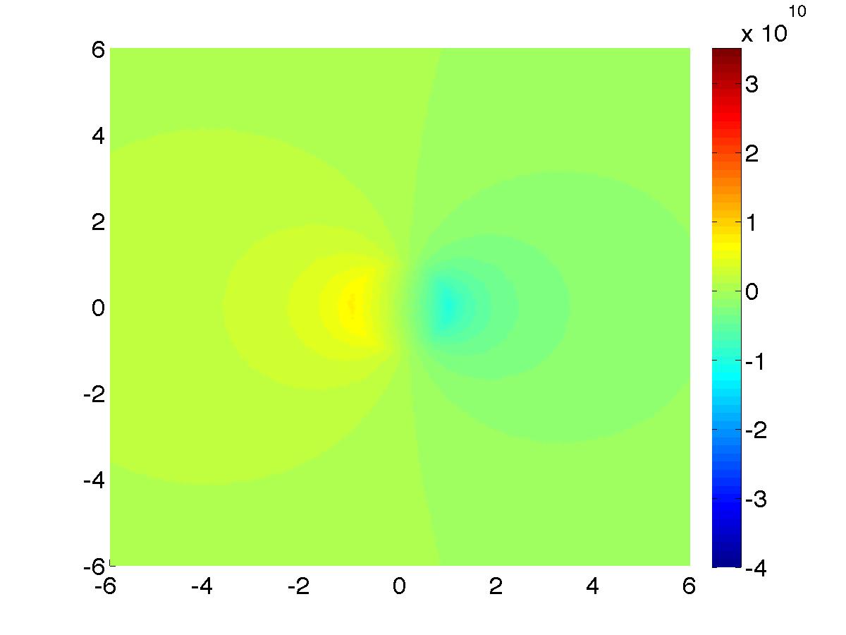
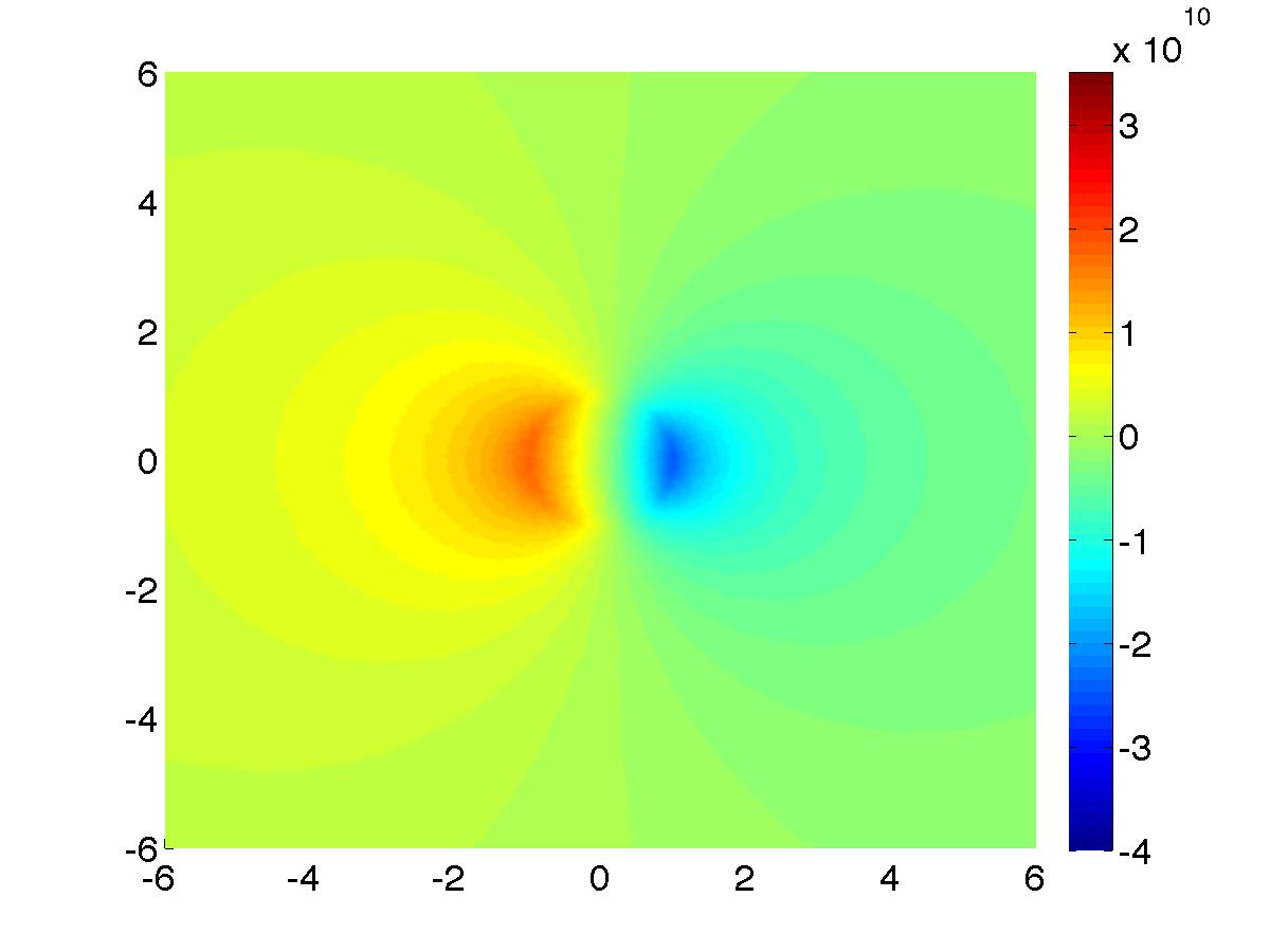
Figure 2: The graphs of $u_{\delta}$ when $\delta=10^{-10},10^{-10.4}$ and $10^{-10.8}$ from the $1^{\rm st}$ to the $3^{\rm rd}$ row. Left: the real part of $u_{\delta}$; Right: the imaginary part of $u_{\delta}.$

Acknowledgement: The authors thank the referees for reading carefully the paper and for useful suggestions, in particular for pointing out the missing point in the proof of Theorems 1 and 2 in the previous version.

References

• [1] H. Ammari, G. Ciraolo, H. Kang, H. Lee, and G. W. Milton, Spectral theory of a Neumann-Poincaré-type operator and analysis of cloaking due to anomalous localized resonance, Arch. Rational Mech. Anal. 218 (2013), 667–692.
• [2] H. Ammari, G. Ciraolo, H. Kang, H. Lee, and G. W. Milton, Anomalous localized resonance using a folded geometry in three dimensions, Proc. R. Soc. Lond. Ser. A469 (2013), 20130048.
• [3] H. Ammari, G. Ciraolo, H. Kang, H. Lee, and G. W. Milton, Spectral theory of a Neumann-Poincaré-type operator and analysis of cloaking due to anomalous localized resonance II, Contemporary Mathematics 615 (2014), 1–14.
• [4] G. Bouchitté and B. Schweizer, Cloaking of small objects by anomalous localized resonance, Quart. J. Mech. Appl. Math. 63 (2010), 437–463.
• [5] R. V. Kohn, J. Lu, B. Schweizer, and M. I. Weinstein, A variational perspective on cloaking by anomalous localized resonance, Comm. Math. Phys. 328 (2014), 1–27.
• [6] G. W. Milton, N. P. Nicorovici, R. C. McPhedran, K. Cherednichenko, and Z. Jacob, A proof of superlensing in the quasistatic regime and limitations of superlenses in this regime due to anomalous localized resonance, Proc. R. Soc. Lond. Ser. A 461 (2005), 3999–4034.
• [7] G. W. Milton and N-A. P. Nicorovici, On the cloaking effects associated with anomalous localized resonance, Proc. R. Soc. Lond. Ser. A 462 (2006), 3027–3059.
• [8] G. W. Milton, N. P. Nicorovici, R. C. McPhedran, K. Cherednichenko, and Z. Jacob, Solutions in folded geometries, and associated cloaking due to anomalous resonance, New J. Phys. 10 (2008), 115021.
• [9] H. M. Nguyen, Asymptotic behavior of solutions to the Helmholtz equations with sign changing coefficients, Trans. Amer. Math. Soc. (2014), http://arxiv.org/abs/1204.1518.
• [10]  , Superlensing using complementary media, Ann. Inst. H. Poincaré Anal. Non Linéaire (2014), http://dx.doi.org/10.1016/j.anihpc.2014.01.004.
• [11]  , Cloaking using complementary media in the quasistatic regime, http://arxiv.org/pdf/1310.5483.pdf.
• [12]  , Cloaking via anomalous localized resonance for doubly complementary media in the quasistatic regime, http://arxiv.org/abs/1407.7977.
• [13] N. A. Nicorovici, R. C. McPhedran, and G. M. Milton, Optical and dielectric properties of partially resonant composites, Phys. Rev. B 49 (1994), 8479–8482.
• [14] J. B. Pendry, Negative refraction makes a perfect lens, Phys. Rev. Lett. 85 (2000), 3966–3969.
• [15] R. A. Shelby, D. R. Smith, and S. Schultz, Experimental verification of a negative index of refraction, Science 292 (2001), 77–79.
• [16] V. G. Veselago, The electrodynamics of substances with simultaneously negative values of $\varepsilon$ and $\mu$, Usp. Fiz. Nauk 92 (1964), 517–526.