Compact (A)dS Boson Stars and Shells

Abstract

We present compact $Q$-balls in an (Anti-)de Sitter background in $D$ dimensions, obtained with a V-shaped potential of the scalar field. Beyond critical values of the cosmological constant $\hat{\Lambda}_{\rm cr}(D)$ compact $Q$-shells arise. By including the gravitational back-reaction, we obtain boson stars and boson shells with (Anti-)de Sitter asymptotics. We analyze the physical properties of these solutions and determine their domain of existence. In four dimensions we address some astrophysical aspects.

I Introduction

Inspired by Wheeler’s quest for the existence of geons Wheeler:1955zz , boson stars were introduced by Feinblum and McKinley Feinblum:1968 , Kaup Kaup:1968zz , and Bonazzola and Ruffini Ruffini:1969qy . In these boson stars the electromagnetic vector field was replaced by some tentative scalar field. With the discovery of a Higgs-like boson last year at the LHC Aad:2012tfa ; Chatrchyan:2012ufa the first fundamental scalar field has been found. But numerous scalar fields have been predicted to exist in high energy physics and cosmology.

Boson stars arise as stationary localized solutions of the coupled Einstein-Klein-Gordon equations Feinblum:1968 ; Kaup:1968zz ; Ruffini:1969qy ; Mielke:1980sa . The physical properties of boson stars depend strongly on the type of scalar field potential employed (see e.g. the review articles Lee:1991ax ; Jetzer:1991jr ; Liddle:1993ha ; Mielke:1997re ; Mielke:2000mh ; Schunck:2003kk ). Mini boson stars arise, when only a mass term is present but no self-interaction. They can reach only relatively small masses. Larger boson stars are obtained, when a repulsive quartic self-interaction is included Colpi:1986ye . For these two types of boson stars gravity is a necessary ingredient.

In contrast, in the presence of a sextic potential one obtains solitonic boson stars Lee:1991ax , which possess a flat space-time limit, where they correspond to non-topological solitons Friedberg:1976me (or $Q$-balls Coleman:1985ki ). Moreover, these solitonic boson stars can reach even higher masses Lee:1991ax .

Here we consider boson stars, which are compact in the sense, that the scalar field of these spherically symmetric configurations is finite inside a ball of radius $r_{\rm o}$, but vanishes identically outside this radius. In this respect the compact $Q$-balls resemble stars Hartmann:2012da . Obtained from a V-shaped self-interaction potential, these compact boson stars also possess a flat space-time limit, compact $Q$-balls Arodz:2008jk ; Arodz:2008nm ; Arodz:2012zh . These represent solutions of the signum-Gordon equation.

The study of scalar fields with a V-shaped self-interaction potential has revealed interesting physical phenomena. When coupled to electromagnetism, the balance of forces allows for shell-like configurations Arodz:2008nm . In these $Q$-shells the scalar field vanishes identically both inside a certain radius $r_{\rm i}$ and outside a certain radius $r_{\rm o}$. The scalar field thus forms a shell of charged matter, $r_{\rm i}<r<r_{\rm o}$.

When coupling these shells to gravity the resulting boson shells possess an empty Minkowski space interior $r<r_{\rm i}$. However, the shells need not be empty in their interior, they can harbour a black hole in there Kleihaus:2009kr . Thus one finds that uniqueness and no-hair theorems for black holes can be avoided in the presence of boson shells Kleihaus:2009kr ; Kleihaus:2010ep .

Whereas these previous studies considered only asymptotically flat solutions, we here include a cosmological constant. On the one hand, a positive cosmological constant is relevant from an observational point of view, since it can model the dark energy of the Universe. Since boson stars are very compact objects that can possess very high densities, they have been suggested as alternatives to supermassive black holes, e.g. in the center of galaxies Schunck:2008xz . Even if that would be excluded by observations (for a discussion see e.g. Broderick:2005xa ) boson stars could still act as toy models for very compact objects, e.g. neutron stars. Such a model of a compact star in a space-time with positive cosmological constant should be a more realistic description of compact stars in the universe, since all observations seem to indicate the existence of a form of dark energy.

A negative cosmological constant, on the other hand, leads to solutions that can be interpreted within the AdS/CFT correspondence Maldacena:1997re ; Witten:1998qj . Recently, the study of boson stars in AdS space-time received increasing attention Sakamoto:1998hq ; Astefanesei:2003qy ; Prikas:2004yw ; Hartmann:2012wa ; Radu:2012yx ; Hartmann:2012gw ; Brihaye:2012ww ; Brihaye:2013hx . This is related to the fact that within the context of a holographic description of superconductors and superfluids Hartnoll:2008vx ; Hartnoll:2008kx ; Horowitz:2008bn (for reviews see Herzog:2009xv ; Hartnoll:2009sz ; Horowitz:2010gk ) the formation of scalar hair on charged solitons in asymptotically AdS has been interpreted as an insulator/superconductor phase transition Horowitz:2010jq ; Brihaye:2011vk . The limit of setting the electric charge of the scalar field $e$ to infinity, which due to the scaling symmetries corresponds to setting Newton’s constant $G$ to zero, is called the “the probe limit” in this context. We adapt this nomenclature here and refer to the case, where the matter field equation is solved in a fixed background, as “the probe limit”. In the opposite limit $e=0$, the gauge symmetry becomes global and the resulting solutions are uncharged solitons in AdS. These are essentially uncharged boson stars and have been suggested to be the holographic description of glueball condensates Horowitz:2010jq .

Boson stars in asymptotic AdS are also of interest from another point of view. It has been suggested that the dynamical formation of a black hole in AdS is the dual description of thermalization in a strongly coupled Quantum Field Theory. As such the stability of AdS space-time was studied with respect to perturbations, and it was conjectured that AdS is unstable under arbitrarily small scalar perturbations and that eventually a black hole would form due to the reflection of the perturbations on the AdS boundary Bizon:2011gg . However, in Buchel:2013uba it was shown that boson stars appear to be nonlinearly stable. If that were true, thermalization in the dual Field Theory would not occur. Hence, boson stars in AdS play an important rôle in the context of the nonlinear (in)stability of AdS space-time, and thus of its dual description.

Here we first consider the set of boson star solutions for various space-time dimensions $D\geq 3$ in the probe limit. Interestingly, the presence of a positive cosmological constant allows for the existence of boson shells without an electromagnetic field. We note, that all objects constructed here are electrically neutral.

By solving the coupled set of the Einstein-signum-Gordon equations, we subsequently determine the domain of existence of the compact (A)dS boson stars and shells in $D\geq 3$ space-time dimensions. We analyze their physical properties and briefly address the stability of the boson stars from a catastrophe theory point of view Kusmartsev:2008py ; Kusmartsev:1992 ; Tamaki:2010zz ; Tamaki:2011zza ; Kleihaus:2011sx . We also address astrophysical aspects of boson stars and boson shells in four dimensions for the physical value of the cosmological constant.

The paper is organized as follows. In section 2 we present the action, the Ansatz, the equations of motion together with the scaling property, the boundary conditions and the global charges. We present the solutions in the probe limit in section 3. The boson stars and shells obtained with the back reaction taken into account are discussed in section 4. We end with our conclusions and an outlook in section 5.

II Model

II.1 Action

We consider the action of a self-interacting complex scalar field $\Phi$ coupled to Einstein gravity in $D$ dimensions

$$S=\int\left[\frac{1}{16\pi G}\left(R-2\Lambda\right)-\frac{1}{2}\left(\partial_{\mu}\Phi\right)^{*}\left(\partial^{\mu}\Phi\right)-U(\left|\Phi\right|)\right]\sqrt{-g}d^{D}x,$$ (1)

with curvature scalar $R$, cosmological constant $\Lambda$, Newton’s constant $G$, and the asterisk denotes complex conjugation. The scalar potential $U$ is chosen as

$$U(|\Phi|)=\lambda|\Phi|.$$ (2)

Variation of the action with respect to the metric and the matter fields leads, respectively, to the Einstein equations

$$G_{\mu\nu}=R_{\mu\nu}-\frac{1}{2}g_{\mu\nu}\left(R-2\Lambda\right)=8\pi GT_{\mu\nu}\$$ (3)

with stress-energy tensor

$$T_{\mu\nu}=g_{\mu\nu}{L}_{M}-2\frac{\partial{L}_{M}}{\partial g^{\mu\nu}}$$ (4)

and the matter field equation,

$$\nabla_{\mu}\nabla^{\mu}\Phi=-\lambda\frac{\Phi}{|\Phi|},$$ (5)

where $\nabla_{\mu}$ denotes the covariant derivative.

Invariance of the action under the global phase transformation

$$\Phi\rightarrow\Phi e^{i\chi}\ ,$$ (6)

leads to the conserved current

$$j^{\mu} = -i\left(\Phi^{*}\partial^{\mu}\Phi-\Phi\partial^{\mu}\Phi^{*}\right)\ ,\ \ \ j^{\mu}_{\ ;\,\mu}=0\ .$$ (7)

and the associated conserved charge $Q$.

II.2 Ansatz

To construct spherically symmetric boson star solutions we employ Schwarzschild-like coordinates and adopt the spherically symmetric metric

$$ds^{2}=g_{\mu\nu}dx^{\mu}dx^{\nu}=-A^{2}Ndt^{2}+N^{-1}dr^{2}+r^{2}d\Omega_{D-2}^{2},$$ (8)

where $d\Omega_{D-2}^{2}$ is the metric on the $D-2$ dimensional unit sphere.

The associated Ansatz for the boson field takes the form

$$\Phi=\phi(r)e^{i\omega t}$$ (9)

with the frequency $\omega$. The conserved scalar charge $Q$

$$Q =- \int j^{t}\left|g\right|^{1/2}d^{D-1}x$$ (10)

is then proportional to $\omega$.

We next introduce dimensionless quantities by

$$r=\hat{r}/\omega\ ,\ \ \phi=\hat{\phi}\lambda/\omega^{2}\ ,\ \ \Lambda=\hat{\Lambda}\omega^{2}\ ,\ \ 8\pi G=\alpha\omega^{4}/\lambda^{2}\ .$$ (11)

Thus the coupling strength of gravity is expressed in terms of the coupling constant $\alpha$. This yields the set of equations

$$\frac{1}{A}A^{\prime} = \frac{2\alpha}{D-2}\hat{r}\left\{\frac{\hat{\phi}^{2}}{N^{2}}+(\hat{\phi}^{\prime})^{2}\right\}\ ,$$ (12)

$$\hat{r}N^{\prime} = (D-3)(1-N)-2\frac{\hat{r}^{2}\hat{\Lambda}}{D-2}-2\frac{\alpha\hat{r}^{2}}{N(D-2)}\left(N^{2}(\hat{\phi}^{\prime})^{2}+2N\hat{\phi}+\hat{\phi}^{2}/A^{2}\right)\ ,$$ (13)

$$\hat{\phi}^{\prime\prime} = \frac{A^{2}N-\hat{\phi}}{A^{2}N^{2}}-\frac{(D-3)+N}{\hat{r}N}\hat{\phi}^{\prime}+\frac{2\hat{r}\hat{\Lambda}}{(D-2)N}\hat{\phi}^{\prime}-4\frac{\hat{r}\alpha}{(D-2)N}\hat{\phi}\hat{\phi}^{\prime}\ .$$ (14)

II.3 Boundary conditions

Let us now specify the boundary conditions for the metric and the boson field. For the metric function $A$ we adopt

$$A(\hat{r}_{o})=1\ ,$$ (15)

where $\hat{r}_{o}$ is the outer radius of the boson star. Since it retains this value to infinity, this fixes the time coordinate. For the metric function $N(\hat{r})$ we require at the origin the regularity condition for globally regular ball-like boson star solutions

$$N(0)=1\ ,$$ (16)

and for globally regular shell-like solutions

$$N(\hat{r}_{\rm i})=1-\frac{2\hat{\Lambda}}{(D-2)(D-1)}\hat{r}_{i}^{2},$$ (17)

where $\hat{r}_{\rm i}$ is the inner radius of the shell.

For boson stars we require for the boson field function one condition at the origin and two conditions at the outer radius $\hat{r}_{o}$

$$\hat{\phi}^{\prime}(0)=0\ ,\ \ \ \hat{\phi}(\hat{r}_{o})=0\ ,\ \ \ \hat{\phi}^{\prime}(\hat{r}_{o})=0\ .$$ (18)

Since this is one condition too many, we introduce another auxiliary differential equation, $\hat{r}_{o}^{\prime}=0$, by treating $\hat{r}_{o}$ as a function. Thus $\hat{r}_{o}$ is constant, but the value of the constant is adjusted in the numerical scheme such that the boundary conditions Eqs. (18) are satisfied. This determines the outer radius of the star.

For boson shells, on the other hand, we require at the inner radius $\hat{r}_{\rm i}$ and at the outer radius $\hat{r}_{\rm o}$ the conditions

$$\hat{\phi}(\hat{r}_{\rm i})=0,\ \ \ \hat{\phi}^{\prime}(\hat{r}_{\rm i})=0,\ \ \ \hat{\phi}(\hat{r}_{\rm o})=0,\ \ \ \hat{\phi}^{\prime}(\hat{r}_{\rm o})=0.$$ (19)

We now also make the ratio of inner and outer radius $\hat{r}_{\rm i}/\hat{r}_{\rm o}$ an auxiliary (constant) variable.

For the numerical computation we introduce the scaled coordinate $x=(\hat{r}-\hat{r}_{i})/(\hat{r}_{o}+\hat{r}_{i})$, such that the inner radius is at $x=0$ and outer radius is at $x=1$.

II.4 Outer solutions

We refer to the solution in the exterior region $\hat{r}\geq\hat{r}_{o}$ as the outer solution of the boson stars and boson shells. In the asymptotically flat case, the outer solution is given by the Schwarzschild solution. In the presence of a cosmological constant the Schwarzschild-de Sitter and Schwarzschild-Anti-de Sitter solutions

$$\hat{\phi}(\hat{r})=0\ ,\ \ A(\hat{r})=1\ ,\ \ N(\hat{r})=1-\frac{2\mu}{\hat{r}^{D-3}}-\frac{2\hat{\Lambda}}{(D-2)(D-1)}\hat{r}^{2}\ ,\ \ \mu=const.$$ (20)

are exact solutions of the ODEs in the exterior region.

Hence the mass parameter of the solutions is given by

$$\mu=\left(1-N(\hat{r}_{o})-\frac{2\hat{r}_{o}^{2}\hat{\Lambda}}{(D-2)(D-1)}\right)\frac{\hat{r}_{o}^{D-3}}{2}\ .$$ (21)

II.5 Inner solutions

Analogously, we refer to the solution in the interior region $\hat{r}\leq\hat{r}_{i}$ as the inner solution of the boson shells. In the asymptotically flat case, the regular inner solution corresponds to flat Minkowski space, whereas in the presence of a cosmological constant the regular inner solutions correspond to either de Sitter or Anti-de Sitter space. Note however, that in general $A(\hat{r})=const.=A_{i}\neq 1$. Thus a rescaling of the time coordinate, $t\to t/A_{i}$, is required to obtain the de Sitter or Anti-de Sitter line element in the standard form.

In principle, we could replace these regular inner solutions by the appropriate black hole solutions, analogously to the asymptotically flat case Kleihaus:2009kr ; Kleihaus:2010ep . Then these inner solutions would correspond to Schwarzschild-de Sitter or Schwarzschild-Anti-de Sitter solutions.

III Probe limit

Here we present the families of solutions in the so called probe limit. Thus we obtain the solutions for vanishing coupling to gravity, i.e., $\alpha=0$, in the respective background.

III.1 $Q$-ball solutions in the Minkowski background

For vanishing cosmological constant the $Q$-ball solutions can be found analytically and expressed in terms of Bessel functions. The $D=4$ solution was given in Arodz:2008jk ; Arodz:2008nm

$$\hat{\phi}(\hat{r})=\left\{\begin{array}[]{clr}\displaystyle 1-\frac{\hat{r}_{o}}{\hat{r}}\frac{\sin\hat{r}}{\sin\hat{r}_{o}}&{\rm if}&0\leq\hat{r}\leq\hat{r}_{o}\\ 0&{\rm if}&\hat{r}\geq\hat{r}_{o}\ .\end{array}\right.$$ (22)

For $D\geq 3$ dimensions this generalizes according to

$$\hat{\phi}(\hat{r})=\hat{r}^{-n}C_{1}J_{n}(\hat{r})+1\ ,\ \ N(\hat{r})=1\ ,\ \ A(\hat{r})=1\ ,$$ (23)

where $n=(D-3)/2$. The constant $C_{1}$ and the outer radius $\hat{r}_{o}$ are determined by the conditions $\hat{\phi}(\hat{r}_{o})=0$ and $\hat{\phi}^{\prime}(\hat{r}_{o})=0$. The latter yields $J_{n+1}(\hat{r}_{o})=0$. Hence $\hat{r}_{o}$ is the smallest non-vanishing zero of $J_{n+1}$. From the first condition it then follows that $C_{1}=-\hat{r}_{o}^{n}/J_{n}(\hat{r}_{o})$. Thus we find

$$\hat{\phi}(\hat{r})=1-\left(\frac{\hat{r}_{o}}{\hat{r}}\right)^{n}\frac{J_{n}(\hat{r})}{J_{n}(\hat{r}_{o})}\ ,\ \ \hat{r}\leq\hat{r}_{o}\ ,\ \ \ \ \hat{\phi}(\hat{r})=0\ ,\ \ \hat{r}>\hat{r}_{o}\ .$$ (24)

The properties of the unique solution in $D=4$ dimensions was discussed in Hartmann:2012da . When going to higher dimensions, the properties of the respective solutions vary only slowly with $D$, and likewise when going to $D=3$. This is seen in Fig. 1, when restricting to a vanishing cosmological constant, $\hat{\Lambda}=0$.

III.2 $Q$-ball solutions in an (Anti-)de Sitter background

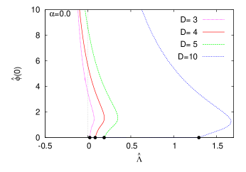
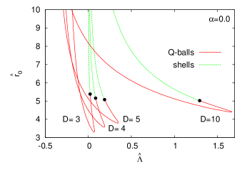
Figure 1: (a) The value of the scalar field at the origin $\hat{\phi}(0)$ and (b) the value of the outer radius $\hat{r}_{o}$ for $Q$-ball and $Q$-shell solutions in the (Anti-)de Sitter background in $D=3$, 4, 5 and 10 dimensions. The black dots label the transition points between $Q$-balls and $Q$-shells.

Let us now consider the $Q$-ball solutions in an (Anti-)de Sitter background in $D$ dimensions. To obtain these solutions, we have solved the scalar field equation in the respective background numerically, employing a Newton-Raphson scheme.

When the scaled cosmological constant $\hat{\Lambda}$ is varied, the solutions change smoothly from the Minkowski background solutions. In Fig. 1 we exhibit the dependence of the solutions on $\hat{\Lambda}$. Here we show the value of the scalar field at the origin $\hat{\phi}(0)$ together with the value of the outer radius $\hat{r}_{o}$ of the solutions for $D=3$, 4, 5 and 10 dimensions.

As the scaled cosmological constant $\hat{\Lambda}$ increases from zero, the value of the scalar field at the origin $\hat{\phi}(0)$ decreases along with the outer radius $\hat{r}_{o}$. Interestingly, there is a maximal value $\hat{\Lambda}_{\rm max}(D)$, which increases with the dimension $D$, for which these solutions exist. At $\hat{\Lambda}_{\rm max}(D)$ a second branch of solutions is encountered. Moving backwards along this second branch the value of the scalar field at the origin $\hat{\phi}(0)$ continues to decrease, until it reaches zero at a critical value $\hat{\Lambda}_{\rm cr}(D)$.

At $\hat{\Lambda}_{\rm cr}(D)$ the solutions change character and $Q$-shells arise. As $\hat{\Lambda}$ decreases further, the inner radius $\hat{r}_{i}$ increases along with the outer radius $\hat{r}_{o}$. In the limit $\hat{\Lambda}\to 0$ the size of the shells diverges while the ratio $\hat{r}_{i}/\hat{r}_{o}$ tends to one. Thus there are no $Q$-shells in a Minkowski or Anti-de Sitter background.

Likewise, when the $Q$-ball solutions are continued to negative values of the cosmological constant, they change smoothly from the Minkowski background solutions, as seen in Fig. 1. As the scaled cosmological constant $\hat{\Lambda}$ decreases from zero, the value of the scalar field at the origin $\hat{\phi}(0)$ increases along with the outer radius $\hat{r}_{o}$ until a minimal value $\hat{\Lambda}_{\rm min}(D)$ encountered, beyond which no such solutions exist. Our data indicate, that $\hat{\Lambda}_{\rm min}(D)=-(D-2)/(2(D-1))$. For a derivation of this limit in $D=4$ dimensions see Appendix A.

IV Back reaction

To study the back reaction of the $Q$-balls and $Q$-shells on the space-time, we have solved the coupled system of equations for the metric and the scalar field numerically. In the following we first discuss the case of $D=4$ dimensions, and then turn to other dimensions.

IV.1 Boson stars and boson shells in $D=4$

IV.1.1 Asymptotically de Sitter boson stars and shells

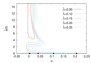
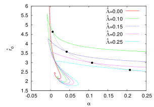
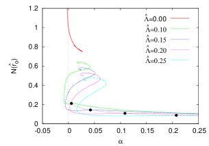
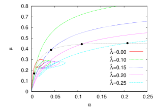
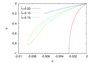
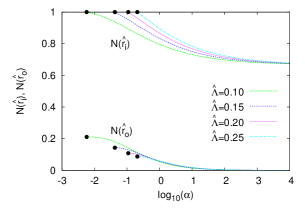
Figure 2: Properties of the boson stars and boson shells in $D=4$ are shown versus $\alpha$ for several values of $\hat{\Lambda}\geq 0$: (a) the scalar field $\hat{\phi}$ at the origin, $\hat{\phi}(0)$, (b) the outer radius $\hat{r}_{o}$, (c) the metric function $A$ at the origin, $A(0)$, (d) the metric function $N$ at the outer radius, $N(\hat{r}_{o})$, (e) the scaled mass $\mu$ for positive $\alpha$, (f) the scaled mass $\mu$ for negative $\alpha$, (g) the ratio of the inner and outer radii $\hat{r}_{i}/\hat{r}_{o}$ for shells only and (h) the values of the metric function at the inner and outer radii, $N(\hat{r}_{i})$ and $N(\hat{r}_{o})$, respectively. The black dots label the transition points between boson stars and boson shells.

Let us start by briefly recalling the properties of the single family of asymptotically flat compact boson star solutions found in Hartmann:2012da . At $\alpha=0$ this family starts from the $Q$-ball solution in the Minkowski background. As seen in Fig. 2, with increasing $\alpha$ the value of the scalar field at the origin $\hat{\phi}(0)$ decreases, until it reaches a finite minimum, and then increases strongly, while $\alpha$ undergoes damped oscillations. In other physical quantities these damped oscillations with respect to $\alpha$ lead to a spiral-like pattern, as seen for the outer radius $\hat{r}_{o}$ or the mass parameter $\mu$. Such a behaviour is typical for boson stars and neutron stars.

Here we have extended this family of compact boson star solutions to negative values of the coupling constant $\alpha$, as seen in Fig. 2. The physical interpretation of the solutions with negative $\alpha$ is that they represent compact solutions made from phantom scalar fields. Thus the negative sign of $\alpha$ can be absorbed by the negative Lagrangian of the phantom field. Ever since the relevance of dark energy for cosmology became apparent, such phantom fields are found ubiquitously in the literature. Moreover, phantom fields also allow for the formation of various types of wormholes.

Let us now turn to compact de Sitter boson stars by increasing the value of $\hat{\Lambda}$ from zero. We demonstrate the effect of a positive cosmological constant on the compact solutions in Fig. 2 by exhibiting the physical properties of such families of solutions for several values of $\hat{\Lambda}$. We see that for finite $\hat{\Lambda}$ the minimum of $\hat{\phi}(0)$ reaches zero. This signals the occurrence of boson shells.

In particular, for a given value of $\hat{\Lambda}$, $\hat{\phi}(0)$ reaches zero at a critical value $\alpha_{\rm cr}(\hat{\Lambda})$. Then for $\alpha>\alpha_{\rm cr}(\hat{\Lambda})$ boson shells exist. $\alpha_{\rm cr}(\hat{\Lambda})$ is exhibited in Fig. 3. For very small positive $\hat{\Lambda}$, the critical value $\alpha_{\rm cr}(\hat{\Lambda})$ is negative. Thus there exist phantom boson shells in this case, which turn into ordinary boson shells, as $\alpha$ increases beyond zero. Extrapolation to $\hat{\Lambda}=0$ indicates, that indeed no shells exist in this limit.

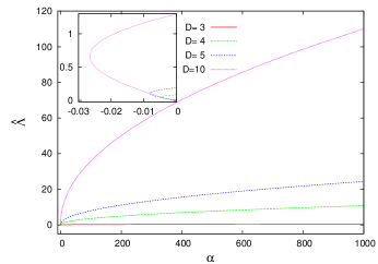
Figure 3: The critical value $\alpha_{\rm cr}$, where the transition from boson stars to boson shells occurs, versus $\hat{\Lambda}$ for $D=3$, 4, 5 and 10 dimensions.

For all values of $\hat{\Lambda}$ the compact boson stars exhibit the characteristic spirals. In Fig. 2 these are seen for the value of the outer radius $\hat{r}_{o}$, the value of the metric function at the outer radius $N(\hat{r}_{o})$ and the value of the scaled mass $\mu$. Interestingly, phantom type boson star solutions exist only for small values of $\hat{\Lambda}$. Since the mass $\mu$ has the same sign as $\alpha$, branches with negative mass exist only for small values of $\hat{\Lambda}$.

Whereas there is an upper bound $\alpha_{\rm max}$ for the compact boson stars, there is no such bound for the boson shells. However, with increasing $\alpha$ their outer radius decreases, and tends to a finite limiting value. At the same time, the ratio of the inner and outer radii $\hat{r}_{i}/\hat{r}_{o}$ increases, and tends to one. Thus the shells become smaller and thinner, while their scaled mass $\mu$ grows. On the other hand, as $\alpha$ is kept fixed while $\hat{\Lambda}$ is decreased, the shells grow in size, while the ratio $\hat{r}_{i}/\hat{r}_{o}$ tends to one. Here in the limit $\alpha\to 0$ the shell size diverges.

IV.1.2 Astrophysical considerations

In the above subsection we have constructed the domain of existence of compact boson stars and boson shells in terms of dimensionless quantities. We can obtain physical solutions with dimensionful quantities by scaling these dimensionless solutions appropriately.

In the case of vanishing cosmological constant we have considered compact stars Hartmann:2012da . In particular, we have shown, that when the mass of these boson stars is on the order of the solar mass then their radius is on the order of ten(s) of kilometers, thus they can correspond in mass and size to neutron stars. Moreover, spirals are also encountered for neutron stars, when they approach the black hole limit.

Concerning their stability, we employ arguments from catastrophe theory Kusmartsev:2008py ; Kusmartsev:1992 ; Tamaki:2010zz ; Tamaki:2011zza ; Kleihaus:2011sx . According to catastrophe theory, the stability changes only at turning points. Thus when starting from a stable configuration, the stability should change at the maximum of the mass. Therefore solutions inside the spiral should be unstable. For neutron stars or ordinary boson stars this has been confirmed by a mode analysis.

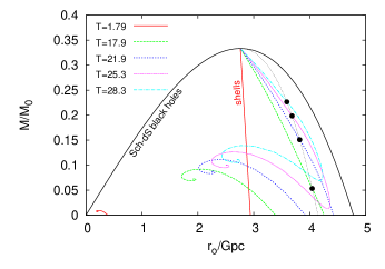
Figure 4: The mass $M$ in units of $M_{0}=c^{2}/(G\sqrt{\Lambda})$ versus the outer radius $\hat{r}_{o}$ in Gigaparsec for several values of $T=2\pi/\omega\propto\sqrt{\hat{\Lambda}}$. The black dots label the transition points between boson stars and boson shells. The black solid curve represents the black hole horizon and the cosmological horizon of the Schwarzschild-de Sitter space-times.

Since the value of the cosmological constant as obtained from cosmology is very small, $\Lambda\lesssim 10^{-52}$ m^-2 in metric units, its presence hardly affects the properties of boson stars that have masses on the order of the mass of the sun. Thus the results for boson stars correspond to those obtained before Hartmann:2012da . However, the presence of a positive cosmological constant, no matter how small, does allow for boson shells. But those boson shells possess cosmological mass and length scales. It would be interesting to see whether such thin boson shells can be associated with voids, i.e. with vast regions of empty space surrounded by a shell of matter.

To see the effect of $\Lambda$ on the compact boson stars let us now consider very big scales. In Fig. 4 we show our scaled results for the mass $M$ in units of $M_{0}=c^{2}/(G\sqrt{\Lambda})$ for boson stars and boson shells versus the outer radius $\hat{r}_{o}$ in units of Gigaparsec. Keeping $\Lambda$ at its physical value, we have translated it into a timescale $T$ via the relation (11), employing units of Gigayears. Shown in addition are the black hole horizon and the cosmological horizon of the corresponding Schwarzschild-de Sitter space-times. Note, that these two horizons coincide for the extremal configuration with the maximum value of the mass.

These Schwarzschild-de Sitter values form the boundary, within which all extended objects must remain. As seen in Fig. 4, the boson stars reside well within these bounds. Note, that since we consider only positive values of the gravitational coupling, i.e., no phantom fields, the boson star curves associated with the smaller values of the parameter $T$ consist of two disconnected parts.

The boson shells, in contrast, exist until they reach this cosmological bound. In particular, all boson shell curves extend precisely to the extremal value of the Schwarzschild-de Sitter curve, where the two horizons coincide. When approaching this limiting configuration, the inner radius of the shells approaches the outer radius. Thus the ratio $\hat{r}_{i}/\hat{r}_{o}$ tends to the value one in this limit. More massive shells cannot exist.

Converting the values in Fig. 4 into numerical values we find that with $\Lambda=10^{-52}{\rm m}^{-2}$ the mass of the boson stars is on the order of $10^{52}$ kg and their radius is on the order of Gpc. These are sizes that are beyond those of galaxies and galaxy clusters. If there were dark matter distributions on such large scales, our solutions would be able to model those. Choosing somewhat smaller values of $T$, on the other hand, we would find sizes relevant for galaxies or galaxy clusters, so that these solutions could be considered to model the dark matter halo of galaxies or the dark matter in galaxy clusters, respectively. Note that in the limit of vanishing mass the radius $r_{o}$ becomes spurious since the non-scaled boson field vanishes identically.

IV.1.3 Asymptotically Anti-de Sitter boson stars

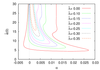
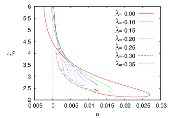
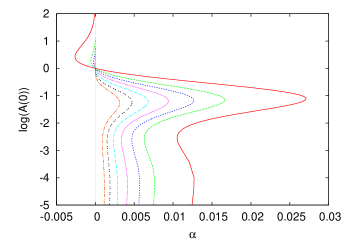
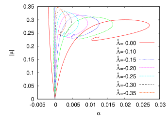
Figure 5: Properties of the boson stars in $D=4$ are shown versus $\alpha$ for several values of $\hat{\Lambda}\leq 0$: (a) the scalar field $\hat{\phi}$ at the origin, $\hat{\phi}(0)$, (b) the outer radius $\hat{r}_{o}$, (c) the metric function $A$ at the origin, $A(0)$, (d) the absolute value of the scaled mass $\mu$.

As expected, compact boson stars exist also for negative values of the cosmological constant. Indeed, the asymptotically Minkowski solutions can be smoothly extended to negative values of $\hat{\Lambda}$, thus yielding asymptotically AdS boson stars. In Fig. 5 we exhibit some of their physical properties versus the coupling constant $\alpha$, for several values of $\hat{\Lambda}$.

We note, that the domain of existence of these compact AdS boson stars decreases with decreasing $\hat{\Lambda}$. This suggests that there is a limiting minimal value for $\hat{\Lambda}$ for compact boson stars. Analogously to the dS case, some of the physical properties of AdS boson stars exhibit damped oscillations with respect to $\alpha$ whereas other properties exhibit spirals. Moreover, as in the dS case, there are phantom boson stars, associated with negative values of $\alpha$.

However, we do not find AdS boson shells. In the AdS case, the scalar field $\hat{\phi}$ never reaches the value zero at the origin, necessary for boson shells to arise. We conclude, that the extra attraction associated with negative $\Lambda$ inhibits the formation of AdS shells even stronger than in the asymptotically flat case, $\Lambda=0$. The existence of shells needs repulsion, that can be provided either by a positive cosmological constant, as seen in the previous subsection, or by the presence of electric charge Arodz:2008jk ; Arodz:2008nm ; Kleihaus:2009kr ; Kleihaus:2010ep .

IV.2 Boson stars and boson shells in $D\neq 4$

Here we consider the domain of solutions and their properties for various space-time dimensions. We have made a complete study for dimensions $D=3$, 5 and 10. Since the dependence on $D$ is mostly rather smooth, we exhibit only a number of selected cases. As an example of a solution, we show an asymptotically de Sitter boson shell solution in Fig. 6.

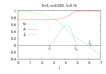
Figure 6: The metric functions $A$, $N$ and the scalar field function $\hat{\phi}$ are shown for the boson shell solution in $D=5$ for parameters $\alpha=0.33$ and $\hat{\Lambda}=0.15$. $r_{c}$ indicates the cosmological horizon.

IV.2.1 Asymptotically de Sitter boson stars and shells

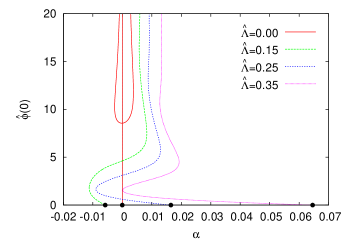
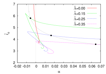
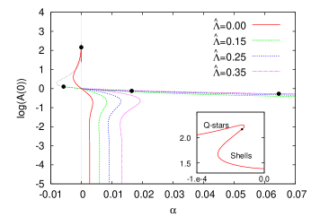
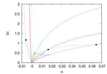
Figure 7: Properties of the boson stars and boson shells in $D=5$ are shown versus $\alpha$ for several values of $\hat{\Lambda}\geq 0$: (a) the scalar field $\hat{\phi}$ at the origin, $\hat{\phi}(0)$, (b) the outer radius $\hat{r}_{o}$, (c) the metric function $A$ at the origin, $A(0)$, (d) the absolute value of the scaled mass $\mu$. The black dots label the transition points between boson stars and boson shells.

We start our discussion by considering boson stars and boson shells in $D=5$ dimensions. Some of their properties are exhibited in Fig. 7, and can be compared to those of Fig. 2.

A surprising feature is that in $D=5$ boson shells seem to exist in the asymptotically flat case, $\hat{\Lambda}=0$. This follows from the additional (almost vertical) line present in Fig. 7 for $\hat{\phi}(0)$. However, since this line is reaching zero for a very small negative value of $\alpha$, those shells are phantom shells. The small branch of phantom shells is seen more clearly in the plot of $A(0)$ in the inset. As $\alpha\to 0$, the size of these phantom shells diverges.

For finite values of $\hat{\Lambda}$, however, we obtain also ordinary dS boson shells. The critical value $\alpha_{\rm cr}(\hat{\Lambda})$ of the transition between the boson stars and shells is seen in Fig. 3. In particular, the resulting phantom dS boson shells continue to exist beyond $\alpha=0$, where they smoothly turn into ordinary boson shells. As in $D=4$, at fixed $\hat{\Lambda}$ with increasing $\alpha$ the outer radius $\hat{r}_{o}$ of these boson shells decreases, tending to a finite limiting value, while their ratio $\hat{r}_{i}/\hat{r}_{o}$ of inner and outer radius increases towards one.

The compact dS boson stars, on the other hand, exist only below a maximal value of $\alpha$, which is either given by the onset of the spiral or by the transition to dS boson shells. For a given $\hat{\Lambda}$, the domain of existence of dS boson stars in $D=5$ with respect to $\alpha$ is smaller than in $D=4$. When going to higher dimensions, this trend continues. In contrast, the domain of existence of phantom dS boson stars increases with increasing $D$.

In $D=3$ dimensions gravity is non-dynamic. Therefore we may expect that boson stars may exhibit a different behavior in $D=3$ dimensions than in higher dimensions.

Let us first inspect the dependence of some of the properties of the compact 3-dimensional objects on $\alpha$ for several values of $\hat{\Lambda}$. Fig. 8 exhibits the scalar field $\hat{\phi}$ at the origin, $\hat{\phi}(0)$, the outer radius $\hat{r}_{o}$, and the scaled mass $\mu$. Here we observe, that indeed some properties of compact boson stars are very different in $D=3$ dimensions. First of all, we notice a maximal value of $\hat{\phi}(0)$, that decreases with increasing $\hat{\Lambda}$. This maximal value is encoutered for negative values of $\alpha$, thus these configurations correspond to phantom boson stars.

As this maximal value of $\hat{\phi}(0)$ two branches of solutions merge. Along one of these branches $\hat{\phi}(0)$ reaches zero. Thus boson shells emerge at the corresponding critical value $\alpha_{\rm cr}$. With increasing $\hat{\Lambda}$ the critical value $\alpha_{\rm cr}$ increases (at least for positive $\alpha_{\rm cr}$), analogously to other dimensions.

The second branch of boson star solutions, however, exhibits a different behaviour from the one observed before. Clearly, the damped oscillations of $\hat{\phi}(0)$ with $\alpha$ are not present. Instead a monotonic decrease of $\hat{\phi}(0)$ with increasing $\alpha$ is observed, and no maximal value of $\alpha$ is encountered. We further observe that for small $\hat{\Lambda}$, $\hat{\phi}(0)$ and the outer radius $\hat{r}_{o}$ depend only weakly on $\hat{\Lambda}$.

The absence of a maximal value of $\alpha$ suggests to consider the dependence of the compact boson stars on $\hat{\Lambda}$, choosing fixed large values of $\alpha$. As can be seen from Figs. 8e and f, for a given $\alpha$ boson star solutions exist only up to a maximal value of $\hat{\Lambda}$, that increases with $\alpha$. Finally, we note that the solutions with $\hat{\Lambda}=0$ are not asymptotically flat, since their mass parameter $\mu$ is finite. This holds for boson stars and boson shells, alike.

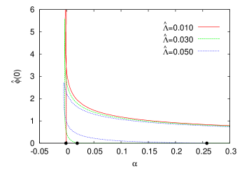
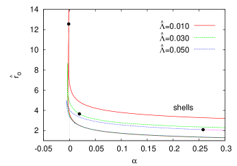
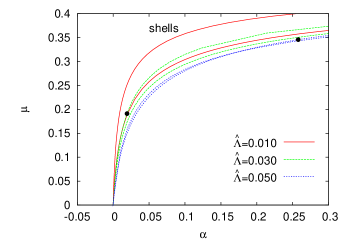
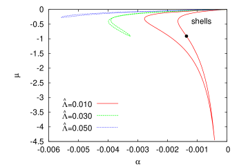
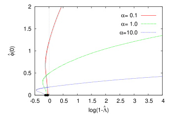
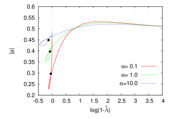
Figure 8: Properties of the boson stars and boson shells in $D=3$: (a) the scalar field $\hat{\phi}$ at the origin, $\hat{\phi}(0)$, (b) the outer radius $\hat{r}_{o}$, (c) and (d) the scaled mass $\mu$ are shown versus $\alpha$ for several values of $\hat{\Lambda}>0$; (e) the scalar field $\hat{\phi}$ at the origin, $\hat{\phi}(0)$, (f) the absolute value of the scaled mass $\mu$ are shown versus $\log(1-\hat{\Lambda})$ for several values of $\alpha$. The black dots label the transition points between boson stars and boson shells.

IV.2.2 Asymptotically Anti-de Sitter boson stars

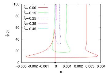
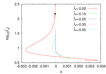
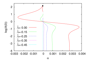
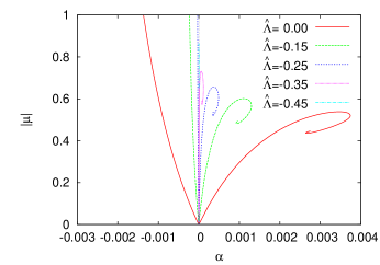
Figure 9: Properties of the boson stars and boson shells in $D=5$ are shown versus $\alpha$ for several values of $\hat{\Lambda}\leq 0$: (a) the scalar field $\hat{\phi}$ at the origin, $\hat{\phi}(0)$, (b) the outer radius $\hat{r}_{o}$, (c) the metric function $A$ at the origin, $A(0)$, (d) the absolute value of the scaled mass $\mu$.

Let us turn finally to AdS boson stars in $D$ dimensions. Some properties of asymptotically AdS boson stars in $D=5$ are exhibited in Fig. 9. As in four dimensions, there are no ordinary AdS boson shells in other than four dimensions. However, there is a very small region of phantom AdS boson shells. This is seen by inspecting the critical curve $\alpha_{\rm cr}(\hat{\Lambda})$ for negative values of $\alpha$ close to zero. Here the critical curve passes negative values of $\hat{\Lambda}$ as well. Like the phantom shells for $\hat{\Lambda}=0$ these phantom AdS shells diverge in size as $\alpha\to 0$.

Otherwise all the basic properties of these AdS solutions in $D=5$ are similar to those of the $D=4$ AdS solutions discussed above. Moreover, we observe only gradual changes with increasing $D$. In particular, the domain of existence of AdS boson stars with respect to $\alpha$ decreases with $D$. Only the domain of phantom AdS shells increases slightly, as seen in Fig. 3.

The lower dimensional case $D=3$ is special again, as can be seen in Figs. 8e and f, where the dependence of $\hat{\phi}(0)$ and $\mu$ on $\hat{\Lambda}$ is shown for several values of $\alpha$. Interestingly, for a given $\alpha$ there is no lower bound of $\hat{\Lambda}$ encountered. Moreover, the mass becomes practically independent of $\alpha$ as $\hat{\Lambda}$ becomes sufficiently small.

When $\hat{\Lambda}$ is fixed instead, while $\alpha$ is varied, no spirals are encountered for the compact 3-dimensional boson stars, whereas spirals are present in all higher dimensions. This was observed before for ordinary boson stars Astefanesei:2003qy . Restricting to positive $\alpha$, there is a maximal value of $\hat{\phi}(0)$ for a given $\hat{\Lambda}$. However, when allowing for phantom fields, a minimal value of $\alpha$ is encountered, beyond which $\hat{\phi}(0)$ increases without bound, while the mass decreases.

V Conclusions and Outlook

We have studied compact boson stars and shells obtained with a V-shaped interaction potential in $D\geq 3$ dimensions. The V-shaped potential confines the scalar field to a finite region, which can be ball-like or shell-like.

In the probe limit, we have given the general analytical solution for $Q$-balls in a Minkowski background. Here no $Q$-shells exist. $Q$-shells arise only beyond a critical value $\Lambda_{\rm cr}(D)>0$ of the cosmological constant, which increases with the number of dimensions $D$. Likewise, $Q$-balls exist only above a minimal value of the cosmological constant, which seems to correspond to $\hat{\Lambda}_{\rm min}(D)=-(D-2)/(2(D-1))$.

Subsequently, we have taken the backreaction into account. The resulting configurations correspond to compact boson stars and boson shells. By solving the coupled set of Einstein-scalar field equations, we have obtained the full set of solutions, subject to Minkowski, de Sitter and Anti-de Sitter asymptotics for a number of space-time dimensions, ranging from 3 to 10.

For any dimension $D\geq 3$ there are compact boson stars with all three types of asymptotics. But concerning their properties, we see a distinct behaviour in three dimensions, that is different from the common behaviour encountered in all higher dimensions. In four and higher dimensions, these boson stars exist in a finite intervall $\alpha_{\rm min}(D,\hat{\Lambda})\leq\alpha\leq\alpha_{\rm max}(D,\hat{\Lambda})$. In constrast, in three dimensions there is no upper bound on the value of $\alpha$.

Also, all boson stars in four and higher dimensions exhibit a spiral-like dependence of the outer radius and the mass on the coupling constant $\alpha$. At the same time, the scalar field value $\hat{\phi}(0)$ exhibits damped oscillations. In constrast, in three dimensions the respective boson star properties do not exhibit such a spiral-like dependence or damped oscillations.

By exploring the parameter space, we also find boson stars for negative values of $\alpha$. These boson stars with negative $\alpha$ correspond to phantom boson stars, since the negative sign of $\alpha$ can be reinterpreted as a negative sign associated with the scalar field in the Lagrangian, and thus with a phantom field. Ample motivation for the consideration of phantom fields is nowadays provided by cosmology.

In constrast to boson stars, boson shells do not exist for Minkowski asymptotics, if there is no additional force present, balancing the gravitational attraction. Consequently, there are no ordinary AdS boson shells. However, dS boson shells do exist. Here the positive cosmological constant provides the necessary repulsion. On the other hand, there exist small regions of phantom AdS shells in more than four dimensions.

In four dimensions we have also considered astrophysical aspects of the compact boson stars and boson shells. While we can always adjust the parameters of the solutions to describe compact astrophysical objects with masses and sizes of neutron stars as discussed in Hartmann:2012da , the influence of the cosmological constant on these objects is negligible, when the physical value of $\Lambda$ is taken. The new feature is, however, that in addition to boson stars there exist also boson shells for positive values of $\Lambda$.

We have then addressed the question, what the properties of such compact objects would be, if we set the scale by the physical value of $\Lambda$. Interestingly, in this case the resulting sets of boson stars reach huge masses and sizes, that are more akin to structures on the largest scales of the universe. The boson shells, on the other hand, can grow in mass until they reach the limit, set by the extremal Schwarzschild-de Sitter solution, for which the event horizon and the cosmological horizon merge.

For negative $\Lambda$ one might be tempted to consider the AdS/CFT correspondence and try to interpret the solutions within this framework. However, all of our solutions are compact. The outer solutions are all given in terms of the Schwarzschild-AdS solutions. Thus the AdS boundary does not feel anything of the solutions except for their mass. Consequently, for such compact solutions the concept of holography does not work. Indeed, lots of different compact objects may sit in the bulk, and if they have the same mass, the boundary does not notice a difference.

As our next step we plan to include rotation Arodz:2009ye . Rotating boson stars are known for non-compact configurations Mielke:2000mh ; Schunck:2003kk ; Yoshida:1997qf ; Kleihaus:2005me ; Kleihaus:2007vk ; Brihaye:2008cg ; Schunck:1996he . Interestingly, their angular momentum $J$ is quantized in terms of their particle number $Q$, $J=nQ$, where $n$ is an integer. We expect, that the rotation of compact boson stars will lead to interesting new features. Moreover, there may be rotating boson shells in the presence of a cosmological constant.

It should also be interesting to construct interacting compact $Q$-balls and $Q$-shells for finite cosmological constant. These should arise in the presence of several complex scalar fields Brihaye:2008cg ; Brihaye:2007tn ; Brihaye:2009yr .

Acknowledgment

We would like to thank Eugen Radu for helpful discussions. We gratefully acknowledge support by the DFG, in particular, also within the DFG Research Training Group 1620 ”Models of Gravity”.

Appendix A AdS solutions in the probe limit

Here we consider the AdS solutions in the probe limit. We introduce the scaled coordiante $\eta=\hat{r}/\ell$, where $\ell=\sqrt{-\frac{(D-2)(D-1)}{2\hat{\Lambda}}}$, and the scaled scalar field $\psi=\hat{\phi}/\hat{\phi}(0)$. This yields for the ODE of the function $\psi$

$$\left(\eta^{m}N\psi^{\prime}\right)^{\prime}+\frac{\ell^{2}\eta^{m}}{N}\psi=\frac{\ell^{2}\eta^{m}}{\hat{\phi}(0)}\ ,$$ (1)

where $m=(D-2)$, $N=1+\eta^{2}$, and prime denotes the derivative with respect to $\eta$.

We rewrite the ODE, Eq. (1), as

$$\psi^{\prime\prime}+p\psi^{\prime}+q\psi=F\ ,\ \ \ {\rm with}\ \ \ p=(\log(\eta^{m}N))^{\prime}\ ,\ \ q=\frac{\ell^{2}}{N^{2}}\ ,\ \ F=\frac{\ell^{2}}{N\hat{\phi}(0)}\ .$$ (2)

If $y_{1}$ is a solution of the homogeneous ODE, then a second independent solution of the homogeneous ODE can be found,

$$y_{2}(\eta)=c_{0}y_{1}(\eta)\int_{0}^{\eta}\frac{d\tau}{\tau^{m}N(y_{1}(\tau))^{2}}\ ,$$ (3)

where $c_{0}$ is a constant.

Now the general solution of the inhomogeneous ODE can be written as

$$\psi=c_{1}y_{1}+c_{2}y_{2}+y_{\rm inh}$$ (4)

where $c_{1}$ and $c_{2}$ are constants and

$$y_{\rm inh}(\eta)=\frac{\ell^{2}}{c_{0}\hat{\phi}(0)}\left[y_{2}(\eta)\int_{0}^{\eta}\tau^{m}y_{1}(\tau)d\tau-y_{1}(\eta)\int_{0}^{\eta}\tau^{m}y_{2}(\tau)d\tau\right]$$ (5)

is a special solution of the inhomogeneous ODE.

Let us assume that $y_{1}$ is regular at $\eta=0$ and $y_{1}(0)=1$. As a consequence the integral in Eq. (3) diverges and $y_{2}$ is singular at $\eta=0$. However, the special solution of the inhomogeneous ODE is regular and vanishes at $\eta=0$. Thus to obtain the regular solution with $\psi(0)=1$ we set $c_{1}=1$ and $c_{2}=0$.

Next we consider the conditions for compact solutions, i.e. $\psi(\eta_{o})=0$ and $\psi^{\prime}(\eta_{o})=0$ at some $\eta_{o}$.

$$\psi(\eta_{o}) = y_{1}(\eta_{o})+\frac{\ell^{2}}{\hat{\phi}(0)}\left[y_{2}(\eta_{o})\int_{0}^{\eta_{o}}\tau^{m}y_{1}(\tau)d\tau-y_{1}(\eta_{0})\int_{0}^{\eta_{o}}\tau^{m}y_{2}(\tau)d\tau\right]=0\ ,$$ (6)

$$\psi^{\prime}(\eta_{o}) = y_{1}^{\prime}(\eta_{o})+\frac{\ell^{2}}{\hat{\phi}(0)}\left[y_{2}^{\prime}(\eta_{o})\int_{0}^{\eta_{o}}\tau^{m}y_{1}(\tau)d\tau-y_{1}^{\prime}(\eta_{0})\int_{0}^{\eta_{o}}\tau^{m}y_{2}(\tau)d\tau\right]=0\ .$$ (7)

The linear superpositions $y_{1}^{\prime}(\eta_{o})\psi(\eta_{o})-y_{1}(\eta_{o})\psi^{\prime}(\eta_{o})=0$ and $y_{2}^{\prime}(\eta_{o})\psi(\eta_{o})-y_{2}(\eta_{o})\psi^{\prime}(\eta_{o})=0$ yield

$$0 = \left[(y_{1}^{\prime}(\eta_{o})y_{2}(\eta_{0})-y_{2}^{\prime}(\eta_{o})y_{1}(\eta_{o})\right]\int_{0}^{\eta_{o}}\tau^{m}y_{1}(\tau)d\tau\ ,$$ (8)

$$0 = \left[(y_{1}^{\prime}(\eta_{o})y_{2}(\eta_{0})-y_{2}^{\prime}(\eta_{o})y_{1}(\eta_{o})\right]\left(1-\frac{\ell^{2}}{\hat{\phi}(0)}\int_{0}^{\eta_{o}}\tau^{m}y_{2}(\tau)d\tau\right)\ ,$$ (9)

respectively, where we set $c_{0}=1$.

Since $y_{1}$ and $y_{2}$ are solutions of the homogeneous ODE it follows that $y_{1}^{\prime}y_{2}-y_{2}^{\prime}y_{1}=c_{h}/(\eta^{m}N)$ for some constant $c_{h}$. As a consequence $\left[(y_{1}^{\prime}(\eta_{o})y_{2}(\eta_{o})-y_{2}^{\prime}(\eta_{o})y_{1}(\eta_{o})\right]\neq 0$ and the conditions (8) and (9) reduce to

$$0 = \int_{0}^{\eta_{o}}\tau^{m}y_{1}(\tau)d\tau\ ,$$ (10)

$$\hat{\phi}(0) = \ell^{2}\int_{0}^{\eta_{o}}\tau^{m}y_{2}(\tau)d\tau\ .$$ (11)

The first equation determines the point $\eta_{o}$ and the second the value of $\hat{\phi}(0)$.

Now we are left with the problem to determine the range of $\ell$ for which solutions of Eq. (10) exist. Although the solutions of the homogeneous ODE can be expressed in terms of hypergeometric functions, we did not succeed to determine the minimal values of $\ell$ in the general case, i.e. in all dimensions.

However, in $D=4$ dimensions the solution $y_{1}$ can be expressed in terms of trigonometric functions,

$$y_{1}=\frac{1}{\ell\eta}\left[\eta\cos(\ell\arctan\eta)-\ell\sin(\ell\arctan\eta)\right]\ ,$$ (12)

which simplifies the problem considerably. Here we consider only $\ell\neq 1$. The case $\ell=1$ needs special treatment.

We will show that Eq. (10) has only a solution $\eta_{o}$ if $\ell>3$. Clearly, the integral in Eq. (10) can only vanish if the integrand possesses (at least) one zero. To analyze this condition we introduce a new coordinate $z=\arctan\eta$, with $0\leq z<\pi/2$, and consider the function

$$\eta\cos(\ell\arctan\eta)-\ell\sin(\ell\arctan\eta) = \tan z\cos(\ell z)-\ell\sin(\ell z)$$ (13)

$$= \left(\sin z\cos(\ell z)-\ell\cos z\sin(\ell z)\right)/\cos z$$ (14)

$$= F(z)/\cos z\ ,$$ (15)

Since $\cos z$ does not change sign on the interval $0\leq z<\pi/2$ it is sufficient to consider the function

$$F=\sin z\cos(\ell z)-\ell\cos z\sin(\ell z)\ .$$ (16)

Now we are left with the question for which values of $\ell$ the function $F$ does not possess a zero.

Let us first restrict to $\ell>1$. Expanding the function $F$ for small values of $z$ we find $F=z\left(1-\ell^{2}\right)+{\cal O}(z^{3})<0$. On the other hand evaluating $F$ at $z=\pi/2$ yields $F(\pi/2)=\cos(\ell\pi/2)>0$ for $3<\ell<5$. Thus, $F(z)$ possesses at least one zero for $3<\ell<5$. Consequently, we can restrict to $1<\ell<3$.

We rewrite Eq. (16) as

$$F = -\frac{1}{2}\left[(\ell-1)\sin(z(\ell+1))+(\ell+1)\sin(z(\ell-1))\right]$$ (17)

$$= -\frac{\ell+1}{2}\left[b\cos a\sin a+\sin(ba)\right]\ ,$$ (18)

where $b=2\frac{\ell-1}{\ell+1}$, $a=z(\ell+1)/2$ are restricted to $0<b<1$ and $0<a<\frac{\pi}{2-b}<\pi$. It can be seen from Fig. 10 that $F(a,b)$ indeed does not a possess a zero in the region $(0,\pi)\times(0,1)$. Consequently there are no compact solutions with $1<\ell<3$.

Now we turn to the case $0<\ell<1$. With $\ell^{\prime}=1/\ell>1$ and $z^{\prime}=z/\ell^{\prime}$ the function $F$ reads

$$F = \sin(\ell^{\prime}z^{\prime})\cos(z^{\prime})-\frac{1}{\ell^{\prime}}\cos(\ell^{\prime}z^{\prime})\sin(z^{\prime})$$ (19)

$$= -\frac{1}{\ell^{\prime}}\left[\sin(z^{\prime})\cos(\ell^{\prime}z^{\prime})-\ell^{\prime}\cos(z^{\prime})\sin(\ell^{\prime}z^{\prime})\right]\ .$$

$$= \frac{1}{2\ell^{\prime}}\left[(\ell^{\prime}-1)\sin(z^{\prime}(\ell^{\prime}+1))+(\ell^{\prime}+1)\sin(z^{\prime}(\ell^{\prime}-1))\right]$$ (20)

Note that now $0<z^{\prime}<\pi/2\ell^{\prime}<\pi/2$. Therefore, $z^{\prime}(\ell^{\prime}+1)<\frac{\pi}{2}(1+1/\ell^{\prime})<\pi$ and $z^{\prime}(\ell^{\prime}-1))<\frac{\pi}{2}(1-1/\ell^{\prime}))<\pi$ imply $\sin(z^{\prime}(\ell^{\prime}+1))>0$ and $\sin(z^{\prime}(\ell^{\prime}-1))>0$. This shows that the function $F$ does not have a zero for $0<\ell<1$.

To conclude, we have found a lower bound for $\ell$, i.e. $\ell_{\rm min}=3$, below which no compact solution can exist. However, this does not prove that solutions exist for $\ell\geq\ell_{\rm min}$, since the condition Eq. (10) is more restrictive than $F=0$ for some $\eta$. Indeed, for $\ell=3$ Eq. (10) yields an equation of the form $x-\tanh(x)=0$, which has no solution for $x>0$. However, consider the case when the function $F(z)$ possesses only one zero on the interval $(0,\pi/2)$ for some $\ell>3$. Denote the zero by $z_{1}$. The condition (10) can then be written as

$$0 = \int_{0}^{z_{o}}F(z)\frac{\sin z}{\cos^{4}z}dz$$ (21)

$$= \int_{0}^{z_{1}}F(z)\frac{\sin z}{\cos^{4}z}dz+\int_{z_{1}}^{z_{o}}F(z)\frac{\sin z}{\cos^{4}z}dz\ .$$

The first integral yields a finite negative contribution, since $F(z)$ is bounded and negative on $(0,z_{1})$. The second integral on the other hand assumes any positive value between zero and infinity, as $z_{o}$ ranges between $z_{1}$ and $\pi/2$, since $F(z)$ is bounded and positive on $(z_{1},\pi/2)$. Consequently, there exists a $z_{o}$ on $(z_{1},\pi/2)$ for which both integrals in Eq. (21) cancel, implying that compact solutions exist for some $\ell>\ell_{\rm min}$.

As an example we computed the exact solution for $\ell=4$. We found

$$\psi(\eta) = \frac{1}{15(1+\eta^{2})^{2}}\left\{15-10\eta^{2}-\eta^{4}\right.$$ (22)

$$\left.-\frac{1}{4\eta\phi_{0}}\left(4\left[(7\eta^{4}+100\eta^{2}-30)\eta-30(5\eta^{2}-1)\arctan\eta\right]\right.\right.$$

$$\left.\left.\ \ \ \ \ \ \ \ \ \ \ \ \ \ \ \ \ \ \ -15(\eta^{4}+10\eta^{2}-15)\eta\log(1+\eta^{2})\right)\right\}\ .$$

For this solution the values $\eta_{o}=7.0657485298$ and $\phi_{0}=20.286677195$ have been computed numerically. Remarkably, they coincide with the corresponding values of our numerically computed solution of the ODE up to eight digits.

Figure 10: The function $F(a,b)$ as given in (18).

References

- (1) J. A. Wheeler, Phys. Rev. 97, 511 (1955).
- (2) D. A. Feinblum, W. A. McKinley, Phys. Rev. 168, 1445 (1968).
- (3) D. J. Kaup, Phys. Rev. 172, 1331 (1968).
- (4) R. Ruffini, S. Bonazzola, Phys. Rev. 187, 1767 (1969).
- (5) G. Aad et al. [ATLAS Collaboration], Phys. Lett. B 716, 1 (2012) [arXiv:1207.7214 [hep-ex]].
- (6) S. Chatrchyan et al. [CMS Collaboration], Phys. Lett. B 716, 30 (2012) [arXiv:1207.7235 [hep-ex]].
- (7) E. W. Mielke and R. Scherzer, Phys. Rev. D 24 (1981) 2111.
- (8) T. D. Lee, Y. Pang, Phys. Rept. 221, 251 (1992).
- (9) P. Jetzer, Phys. Rept. 220, 163 (1992).
- (10) A. R. Liddle, M. S. Madsen, Int. J. Mod. Phys. D1, 101 (1992).
- (11) E. W. Mielke, F. E. Schunck, 8th Marcel Grossmann Meeting (MG 8), Jerusalem, Israel, 22-27 Jun 1997, Pt.B 1607 [gr-qc/9801063].
- (12) E. W. Mielke and F. E. Schunck, Nucl. Phys. B 564, 185 (2000). [arXiv:gr-qc/0001061].
- (13) F. E. Schunck, E. W. Mielke, Class. Quant. Grav. 20, R301 (2003). [arXiv:0801.0307 [astro-ph]].
- (14) M. Colpi, S. L. Shapiro, I. Wasserman, Phys. Rev. Lett. 57, 2485 (1986).
- (15) R. Friedberg, T. D. Lee and A. Sirlin, Phys. Rev. D 13, 2739 (1976).
- (16) S. R. Coleman, Nucl. Phys. B 262, 263 (1985) [Erratum-ibid. B 269, 744 (1986)].
- (17) B. Hartmann, B. Kleihaus, J. Kunz and I. Schaffer, Phys. Lett. B 714, 120 (2012) [arXiv:1205.0899 [gr-qc]].
- (18) H. Arodz and J. Lis, Phys. Rev. D 77, 107702 (2008). [arXiv:0803.1566 [hep-th]].
- (19) H. Arodz and J. Lis, Phys. Rev. D 79, 045002 (2009). [arXiv:0812.3284 [hep-th]].
- (20) H. Arodz, J. Karkowski and Z. Swierczynski, Acta Phys. Polon. B 43 (2012) 79 [arXiv:1201.2279 [hep-th]].
- (21) B. Kleihaus, J. Kunz, C. Lammerzahl and M. List, Phys. Lett. B 675, 102 (2009). [arXiv:0902.4799 [gr-qc]].
- (22) B. Kleihaus, J. Kunz, C. Lammerzahl and M. List, Phys. Rev. D 82, 104050 (2010). [arXiv:1007.1630 [gr-qc]].
- (23) F. E. Schunck and A. R. Liddle, Lect. Notes Phys. 514, 285 (1998) [arXiv:0811.3764 [astro-ph]].
- (24) A. E. Broderick and R. Narayan, Astrophys. J. 638 (2006) L21 [astro-ph/0512211].
- (25) J. M. Maldacena, Adv. Theor. Math. Phys. 2, 231 (1998) [hep-th/9711200].
- (26) E. Witten, Adv. Theor. Math. Phys. 2, 253 (1998) [hep-th/9802150].
- (27) K. Sakamoto and K. Shiraishi, JHEP 9807, 015 (1998) [gr-qc/9804067].
- (28) D. Astefanesei and E. Radu, Nucl. Phys. B 665 (2003) 594 [gr-qc/0309131].
- (29) A. Prikas, Gen. Rel. Grav. 36 (2004) 1841 [hep-th/0403019].
- (30) B. Hartmann and J. Riedel, Phys. Rev. D 86, 104008 (2012) [arXiv:1204.6239 [hep-th]].
- (31) E. Radu and B. Subagyo, Phys. Lett. B 717, 450 (2012) [arXiv:1207.3715 [gr-qc]].
- (32) B. Hartmann and J. Riedel, Phys. Rev. D 87, 044003 (2013) [arXiv:1210.0096 [hep-th]].
- (33) Y. Brihaye, B. Hartmann and S. Tojiev, Phys. Rev. D 87, 024040 (2013) [arXiv:1210.2268 [gr-qc]].
- (34) Y. Brihaye, B. Hartmann and S. Tojiev, Class. Quant. Grav. 30, 115009 (2013) [arXiv:1301.2452 [hep-th]].
- (35) S. A. Hartnoll, C. P. Herzog and G. T. Horowitz, Phys. Rev. Lett. 101, 031601 (2008) [arXiv:0803.3295 [hep-th]].
- (36) S. A. Hartnoll, C. P. Herzog and G. T. Horowitz, JHEP 0812, 015 (2008) [arXiv:0810.1563 [hep-th]].
- (37) G. T. Horowitz and M. M. Roberts, Phys. Rev. D 78, 126008 (2008) [arXiv:0810.1077 [hep-th]].
- (38) C. P. Herzog, J. Phys. A 42, 343001 (2009) [arXiv:0904.1975 [hep-th]].
- (39) S. A. Hartnoll, Class. Quant. Grav. 26, 224002 (2009) [arXiv:0903.3246 [hep-th]].
- (40) G. T. Horowitz, Lect. Notes Phys. 828, 313 (2011) [arXiv:1002.1722 [hep-th]].
- (41) G. T. Horowitz and B. Way, JHEP 1011 (2010) 011 [arXiv:1007.3714 [hep-th]].
- (42) Y. Brihaye and B. Hartmann, Phys. Rev. D 83 (2011) 126008 [arXiv:1101.5708 [hep-th]].
- (43) P. Bizon and A. Rostworowski, Phys. Rev. Lett. 107 (2011) 031102 [arXiv:1104.3702 [gr-qc]].
- (44) A. Buchel, S. L. Liebling and L. Lehner, Phys. Rev. D 87, 123006 (2013) [arXiv:1304.4166 [gr-qc]].
- (45) F. V. Kusmartsev, E. W. Mielke, F. E. Schunck, Phys. Rev. D43, 3895 (1991). [arXiv:0810.0696 [astro-ph]].
- (46) F. V. Kusmartsev, F. E. Schunck, Physica B178, 24 (1992).
- (47) T. Tamaki, N. Sakai, Phys. Rev. D81, 124041 (2010). [arXiv:1105.1498 [gr-qc]].
- (48) T. Tamaki, N. Sakai, Phys. Rev. D83, 044027 (2011). [arXiv:1105.2932 [gr-qc]].
- (49) B. Kleihaus, J. Kunz and S. Schneider, Phys. Rev. D 85, 024045 (2012) [arXiv:1109.5858 [gr-qc]].
- (50) N. Itoh, Prog. Theor. Phys. 44, 291 (1970).
- (51) E. Witten, Phys. Rev. D30, 272-285 (1984).
- (52) E. Farhi, R. L. Jaffe, Phys. Rev. D30, 2379 (1984).
- (53) C. Alcock, E. Farhi and A. Olinto, Astrophys. J. 310, 261 (1986).
- (54) J. Lis, Acta Phys. Polon. B 41, 629 (2010). [arXiv:0911.3423 [hep-th]].
- (55) H. Arodz, J. Karkowski and Z. Swierczynski, Phys. Rev. D 80, 067702 (2009). [arXiv:0907.2801 [hep-th]].
- (56) S. Yoshida and Y. Eriguchi, Phys. Rev. D 56, 762 (1997).
- (57) B. Kleihaus, J. Kunz and M. List, Phys. Rev. D 72, 064002 (2005). [arXiv:gr-qc/0505143].
- (58) B. Kleihaus, J. Kunz, M. List and I. Schaffer, Phys. Rev. D 77, 064025 (2008). [arXiv:0712.3742 [gr-qc]].
- (59) Y. Brihaye and B. Hartmann, Phys. Rev. D 79, 064013 (2009). [arXiv:0812.3968 [hep-ph]].
- (60) F. E. Schunck and E. W. Mielke, Phys. Lett. A 249 (1998) 389.
- (61) Y. Brihaye and B. Hartmann, Nonlinearity 21, 1937 (2008). [arXiv:0711.1969 [hep-th]].
- (62) Y. Brihaye, T. Caebergs, B. Hartmann and M. Minkov, Phys. Rev. D 80, 064014 (2009). [arXiv:0903.5419 [gr-qc]].