A two-level method for Mimetic Finite Difference discretizations of elliptic problems

Abstract

We propose and analyze a two-level method for mimetic finite difference approximations of second order elliptic boundary value problems. We prove that two-level algorithm is uniformly convergent, i.e., the number of iterations needed to achieve convergence is uniformly bounded independently of the characteristic size of the underling partition. We also show that the resulting scheme provides a uniform preconditioner with respect to the number of degrees of freedom. Numerical results that validate the theory are also presented.

Keywords: Mimetic finite difference discretizations, two-level preconditioners

1 Introduction

Thanks to its great flexibility in dealing with very general meshes and its capability of preserving the fundamental properties of the underlying physical model, the mimetic finite difference (MFD) method has been successfully employed, in approximately the last ten years, to solve a wide range of problems. Mimetic methods for the discretization of diffusion problems in mixed form are presented in [40, 41, 25, 28, 26, 27]. The primal form of the MFD method is introduced and analyzed in [23, 15]. Convection–diffusion problems are considered in [32, 11], while the problem of modeling flows in porous media is addressed [48]. Mimetic discretizations of linear elasticity and the Stokes equations are presented in [10] and [12, 14, 13], respectively. MFD methods have been used in the solution of Reissner-Mindlin plate equations [20], and electromagnetic [22, 47] equations. Numerical techniques to improve further the capabilities of MFD discretizations such that a posteriori error estimators [9, 17, 1] and post-processing techniques [31] have been also developed. The application of the MFD method to nonlinear problems (variational inequalities and quasilinear elliptic equations) and constrained control problems governed by linear elliptic PDEs is even more recent, see [3] for a review. More precisely, in [4, 2] a MFD approximation of the obstacle problem, a paradigmatic example of variational inequality, is considered. The question whether the MFD method is well suited for the approximation of optimal control problems governed by linear elliptic equations and quasilinear elliptic equations is addressed in [5] and [6], respectively. Recently, in [18], the mimetic approach has been recast as the virtual element method (VEM), cf. also [29, 19]. Nevertheless, the issue of developing efficient solution techniques for the (linear) systems of equations arising from MFD discretizations haas not been addressed right now. The main difficulty in the development of optimal multilevel solution methods relies on the construction of consistent coarsening procedures which are non-trivial on grids formed by more general polyhedra. We refer to [46, 50, 45] for recent works on constructing coarse spaces with approximation properties in the framework of the agglomeration multigrid method. Very recently, using the techniques of [30, 8], a multigrid algorithm for Discontinuous Galerkin methods on polygonal and polyhedral meshes has been analyzed in [7].

The aim of this paper is to develop an efficient two-level method for the solution of the linear systems of equations arising from MFD discretizations of a second order elliptic boundary value problem. We prove that the two-level algorithm that rely on the construction of suitable prolongation operators between a hierarchy of meshes is uniformly convergent with respect to the characteristic size of the underling partition. We also show that the resulting scheme provides a uniform preconditioner, i.e., the number of Preconditioned Conjugate Gradient (PCG) iterations needed to achieve convergence up to a (user-defined) tolerance is uniformly bounded independently of the number of degrees of freedom. An important observation is that for unstructured grids a two-level (and multilevel) method is optimal if the number of nonzeroes in the coarse grid matrices is under control. This is important for practical applications and one of the main features of the method proposed here is that we modify the coarse grid operator so that the number of nonzeroes in the corresponding coarse grid matrix is under control. This in turn complicates the analysis of the preconditioner, since we need to account for the fact that the bilinear form on the coarse grid is no longer a restriction of the fine grid bilinear form.

The layout of the paper is as follows. In Section 2 we introduce the model problem and its mimetic finite difference discretization. The solvability of the discrete problem is discussed also in this section and further, spectral bounds of the stiffness matrix arising form MFD discretization are provided in Section 2.3. Our two-level preconditioners are described and analyzed in Section 3. Finally, in Section 4 we present numerical results to validate the theoretical estimates of the previous sections and to test the practical performance of our algorithms.

2 Model problem and its mimetic discretization

Let $\Omega$ be an open, bounded Lipschitz polygon in $\mathbb{R}^{2}$. Using the standard notation for the Sobolev spaces, we consider the following variational problem: Find $u\in H^{1}_{0}(\Omega)$ such that

$$\int_{\Omega}{\kappa(\bm{x})\nabla u\cdot\nabla v\textrm{\, d}\bm{x}}=\int_{\Omega}{f\leavevmode\nobreak\ v\textrm{\, d}\bm{x}},\quad\mbox{for all}\quad v\in H^{1}_{0}(\Omega).$$ (1)

Here, $f\in L^{2}(\Omega)$ and we assume that the function $\kappa(\bm{x})$ is a piecewise constant function, bounded and strictly positive, namely, there exist $\kappa_{\star},\kappa^{\star}>0$ such that $\kappa_{\star}\leq\kappa(\bm{x})\leq\kappa^{\star}$.

We now briefly review the mimetic discretization method for problem (1) presented in [24] and extended to arbitrary polynomial order in [16]. In the following, to avoid the proliferation of constants, by $\lesssim$ we denote an upper bound that holds up to an unspecified positive constant. Moreover, $(\cdot,\cdot)$ will denote the Euclidean scalar product in $\ell^{2}(\mathbb{R}^{n})$, and $\|\cdot\|$ its induced norm. Finally, $(\cdot,\cdot)_{X}$ and $\|\cdot\|_{X}$, will denote the inner product and the norm generated by a symmetric, positive definite matrix $X$, repsectively.

2.1 Domain partitioning

We partition $\Omega$ as union of connected, convex polygonal subdomains with non-empty interior. We denote this partition with $\Omega_{H}$, and assume it is conforming, i.e., the intersection of the closure of two different elements is either empty or is a union of vertices or edges. Notice that assuming that $\Omega_{H}$ is made of convex elements is not restrictive and an algorithm for such decomposition into a small (close to minimum) number of convex polygons is presented in [33]. For each polygon $E\in\Omega_{H}$, $|E|$ denotes its area, $H_{E}$ denotes its diameter and $H=\max_{E\in\Omega_{H}}H_{E}$ is the characteristic size of the partition $\Omega_{h}$. The set of vertices and edges of the partition is denoted by ${\mathcal{N}}_{H}$ and ${\mathcal{E}}_{H}$, respectively. The vertices and edges of a particular element $E$ are denoted by ${\mathcal{N}}_{H}^{E}$ and ${\mathcal{E}}_{H}^{E}$, respectively. A generic vertex will be denoted by ${\mathsf{v}}$, and a generic edge by $e$. We also assume that $\Omega_{H}$ satisfies the following assumptions, cf.  [24].

Assumption 1.

There exists an integer number $N_{s}$, independent of $H$, such that any polygon $E\in\Omega_{H}$ admits a decomposition into at most $N_{s}$ shape-regular triangles;

Assumption 1 implies the following properties which we use later, cf. [24] for more details.

1. The number of vertices and edges of every polygon $E$ of $\Omega_{H}$ is uniformly bounded.

2. For every $E\in\Omega_{H}$ and for every edge $e$ of $E$, it holds $H_{E}\lesssim|e|$ and $H_{E}^{2}\lesssim|E|$.

3. The following trace inequality holds

   $$\|\psi\|_{L^{2}(e)}^{2}\lesssim H_{E}^{-1}\|\psi\|_{L^{2}(E)}^{2}+H_{E}\left|\psi\right|_{H^{1}(E)}^{2} \forall\,\psi\in H^{1}(E).$$

4. For every $E$ and for every function $\psi\in H^{m}(E)$, $m\in\mathbb{N}$, there exists a polynomial $\psi_{k}$ of degree at most $k$ on $E$ such that

   $$\left|\psi-\psi_{k}\right|_{H^{l}(E)}\lesssim H_{E}^{m-l}\left|\psi\right|_{H^{m}(E)}$$

   for all integers $0\leq l\leq m\leq k+1$.

We then consider a fine partition $\Omega_{h}$ obtained after a uniform refinement of $\Omega_{H}$, according to the procedure described in Algorithm 1.

Algorithm 1 Refinement algorithm, see Figure 1.

1:for all polygons $E\in\Omega_{H}$ do

2:     Introduce the point ${\bf x}_{E}\in E$ defined as

$${\bf x}_{E}=\frac{1}{n_{E}}\sum_{{\mathsf{v}}\in{\mathcal{N}}_{H}^{E}}{\bf x}({\mathsf{v}})\ ,$$

where $n_{E}$ is the number of vertexes ${\mathsf{v}}$ of $E$, and ${\bf x}({\mathsf{v}})$ is the position vector of the vertex ${\mathsf{v}}$.

3:     Subdivide $E$ of $\Omega_{H}$ by connecting each midpoint ${\mathsf{v}_{m}}={\mathsf{v}_{m}}(e)$ of each edge $e\in{\mathcal{E}}_{H}^{E}$ with the point ${\bf x}_{E}$, see Figure 1.

4:end for

Figure 1: Refinement strategy: a coarse element $E\in\Omega_{H}$ is subdivided into sub-elements. Circles denote the coarse vertexes in ${\mathcal{N}}_{H}$, while squares refer to additional vertexes in ${\mathcal{N}}_{h}$.

Notice that, by construction, the grid $\Omega_{h}$ automatically satisfies properties $(\textsf{M1})-(\textsf{M4})$. As before, the diameter of an element $E\in\Omega_{h}$ will be denoted by $h_{E}$, and we set $h=\max_{E\in\Omega_{h}}h_{E}$. Accordingly, ${\mathcal{N}}_{h}$ and ${\mathcal{E}}_{h}$ will denote the sets of vertices and edges of $\Omega_{h}$, respectively. We also observe that, according to Algorithm 1, the edge midpoints ${\mathsf{v}_{m}}(e)$ and the points ${\bf x}_{E}$ become additional vertexes in the new mesh ${\Omega}_{h}$, i.e.,

$${{\mathcal{N}}}_{h}={\mathcal{N}}_{H}\cup\{{\mathsf{v}_{m}}(e)\}_{e\in{\mathcal{E}}_{H}}\cup\{{\bf x}_{E}\}_{E\in\Omega_{H}}.$$ (2)

Finally, we assume that the jumps in $\kappa(x)$ are aligned with the finest grid and we denote by $\kappa_{E}$ the coefficient value in the polygon $E\in\Omega_{h}$.

2.2 Mimetic finite difference discretization

In this section we describe the MDF approximation to problem (1) on the finest grid $\Omega_{h}$. We begin by introducing the discrete approximation space $V_{h}$: any vector $v_{h}\in V_{h}$ is given by $v_{h}=\{v_{h}({\mathsf{v}})\}_{{\mathsf{v}}\in{\mathcal{N}}_{h}}$, where $v_{h}({\mathsf{v}})$ is a real number associated to the vertex ${\mathsf{v}}\in{\mathcal{N}}_{h}$. To enforce boundary conditions, for all nodes of the mesh which lay on the boundary we set $v_{h}({\mathsf{v}})=0$. Denoting by $N_{h}$ the cardinality of ${\mathcal{N}}_{h}$, we have that $V_{h}\equiv\mathbb{R}^{N_{h}}$.

The mimetic discretization of problem (1) reads: Find $u_{h}\in V_{h}$ such that

$$a_{h}(u_{h},v_{h})=(f_{h},v_{h}) \forall v_{h}\in V_{h}.$$ (3)

where

$$(f_{h},v_{h})=\sum_{E\in\Omega_{h}}\bar{f}|_{E}\sum_{{\mathsf{v}}_{i}\in{\mathcal{N}}_{h}^{E}}v_{h}({\mathsf{v}}_{i})\>\omega_{E}^{i},$$

with $\bar{f}|_{E}$ is the average of $f$ over $E$ and $\omega_{E}^{i}$ are positive weights such that $\sum_{i}\omega_{E}^{i}=|E|$. The bilinear form $a_{h}(\cdot,\cdot):V_{h}\times V_{h}\to\mathbb{R}$ is defined as follows:

$$a_{h}(v_{h},w_{h})=\sum_{E\in\Omega_{h}}a_{h}^{E}(v_{h},w_{h}) \forall v_{h},w_{h}\in V_{h},$$

where, for each $E\in\Omega_{h}$, $a_{h}^{E}(\cdot,\cdot)$ is a symmetric bilinear form that can be constructed in a simple algebraic way, as shown in [24, 4]. We next recall this algebraic expression and use it to show that (3) is well posed. For any $E\in\Omega_{h}$ let $n_{E}$ be the number of its vertexes and let $\mathsf{A}^{E}_{h}\in{\mathbb{R}}^{n_{E}\times n_{E}}$ be the symmetric matrix representing the local bilinear form $a_{h}^{E}(\cdot,\cdot)$, i.e.,

$$(\mathsf{A}^{E}_{h}v_{h},w_{h})=a_{h}^{E}(v_{h},w_{h}) \forall v_{h},w_{h}\in V_{h}.$$

We define

$$\mathsf{A}^{E}_{h}=\frac{1}{\kappa_{E}\left|E\right|}\mathsf{R}\mathsf{R}^{T}+s\>\mathsf{P}\ ,$$ (4)

with $s=\textrm{trace}(\frac{1}{\kappa_{E}\left|E\right|}\mathsf{R}\mathsf{R}^{T})>0$ a scaling factor. The matrix $\mathsf{P}$ is defined as $\mathsf{P}={\mathsf{I}}-\mathsf{N}(\mathsf{N}^{T}\mathsf{N})^{-1}\mathsf{N}^{T}$, where

$$\mathsf{N}=\begin{pmatrix}1&x_{1}-\bar{x}_{E}&y_{1}-\bar{y}_{E}\\ 1&x_{2}-\bar{x}_{E}&y_{2}-\bar{y}_{E}\\ 1&x_{3}-\bar{x}_{E}&y_{3}-\bar{y}_{E}\\ \vdots&\vdots\\ 1&x_{n_{E}}-\bar{x}_{E}&y_{n_{E}}-\bar{y}_{E}\\ \end{pmatrix},$$ (5)

being ${\mathsf{v}}_{1}=(x_{1},y_{1}),\ldots,{\mathsf{v}}_{n_{E}}=(x_{n_{E}},y_{n_{E}})$ and $(\bar{x}_{E},\bar{y}_{E})$ the vertexes and the center of mass of $E$, respectively. The matrix $\mathsf{R}$ has the following form

$$\mathsf{R} =\frac{\kappa_{E}}{2}\begin{pmatrix}0&y_{2}-y_{n_{E}}&x_{n_{E}}-x_{2}\\ 0&y_{3}-y_{1}&x_{1}-x_{3}\\ 0&y_{4}-y_{2}&x_{2}-x_{4}\\ \vdots&\vdots&\vdots\\ 0&y_{1}-y_{n_{E}-1}&x_{n_{E}-1}-x_{1}\end{pmatrix}.$$

Note that, by construction, it holds $\mathsf{A}^{E}_{h}\mathsf{N}=\mathsf{R}$.

We now prove a result which is basic in showing solvability of the discrete problem.

Lemma 2.1.

The matrix $\mathsf{A}^{E}_{h}$ is positive semidefinite. Moreover, $\mathsf{A}^{E}_{h}z=0$ if and only if $z=(\alpha,\ldots,\alpha)^{T}$ for some $\alpha\in{\mathbb{R}}$.

Proof.

For any $z\in\mathbb{R}^{n_{E}}$, using that $\mathsf{P}^{2}=\mathsf{P}$ and $\mathsf{P}^{T}=\mathsf{P}$, we have

$$(\mathsf{A}^{E}_{h}z,z)=\frac{1}{\kappa_{E}\left|E\right|}(\mathsf{R}\mathsf{R}^{T}z,z)+s(\mathsf{P}z,z)=\frac{1}{\kappa_{E}\left|E\right|}\|\mathsf{R}^{T}z\|^{2}+s\|\mathsf{P}z\|^{2}\geq 0.$$ (6)

We next show that $\mathsf{A}^{E}_{h}z=0$ if and only if $z=(\alpha,\ldots,\alpha)^{T}$ for some $\alpha\in{\mathbb{R}}$. One direction of the proof is easy. Indeed, taking $z=(\alpha,\ldots,\alpha)^{T}$ for $\alpha\in\mathbb{R}$, then

$$z=\mathsf{N}\begin{pmatrix}\alpha\\ 0\\ 0\end{pmatrix},$$

and hence

$$\mathsf{A}^{E}_{h}z=\mathsf{A}^{E}_{h}\mathsf{N}\begin{pmatrix}\alpha\\ 0\\ 0\end{pmatrix}=\mathsf{R}\begin{pmatrix}\alpha\\ 0\\ 0\end{pmatrix}=0.$$

To prove the other direction, let us assume that $\mathsf{A}^{E}_{h}z=0$. Equation (6) clearly implies that $\mathsf{R}^{T}z=0$ and $\mathsf{P}z=0$. From $\mathsf{P}z=0$, we conclude that $z\in\operatorname{Range}(\mathsf{N})$, and, hence, $z=\mathsf{N}\widetilde{z}$ for some $\widetilde{z}=(\widetilde{z}_{1},\widetilde{z}_{2},\widetilde{z}_{3})^{T}\in\mathbb{R}^{3}$. This yields

$$\mathsf{R}\widetilde{z}=\mathsf{A}^{E}_{h}\mathsf{N}\widetilde{z}=\mathsf{A}^{E}_{h}z=0.$$

We now want to show that $(\widetilde{z}_{1},\widetilde{z}_{2},\widetilde{z}_{3})^{T}=(\alpha,0,0)^{T}$ for some $\alpha\in\mathbb{R}$. Indeed, denoting by $\bm{\nu}_{E}^{e}$ the unit normal vector to the edge $e$ pointing outside of $E$, the identity $\mathsf{R}\widetilde{z}=0$, shows that $(\widetilde{z}_{2},\widetilde{z}_{3})^{T}\cdot\bm{\nu}_{E}^{{\mathsf{e}}_{i}}=0$ for $i=1,\ldots,n_{E}$. As at least two of the normal vectors $\{\bm{\nu}_{E}^{{\mathsf{e}}_{i}}\}_{i=1}^{n_{E}}$ are linearly independent, this implies that $\widetilde{z}_{2}=\widetilde{z}_{3}=0$. Finally, the proof is concluded by setting $\widetilde{z}_{1}=\alpha$, $\widetilde{z}_{2}=\widetilde{z}_{3}=0$, and computing $\mathsf{N}\widetilde{z}$ which yields $z=\mathsf{N}\widetilde{z}=(\alpha,\ldots,\alpha)^{T}$. To show that $\mathsf{A}^{E}_{h}$ is positive definite on the orthogonal complement of the constant vectors, we have to show that

$$(\mathsf{A}^{E}_{h}z,z)>0,$$

for any $z=(u_{1},u_{2},u_{3})^{T}$ such that $u_{1}+u_{2}+u+3=0$. For such $z$ we have $\|\mathsf{R}^{T}z\|\neq 0$ and $\|\mathsf{P}z\|\neq 0$, and, hence, (6) gives

$$(\mathsf{A}^{E}_{h}z,z)=\frac{1}{\kappa_{E}\left|E\right|}\|\mathsf{R}^{T}z\|^{2}+s\|\mathsf{P}z\|^{2}>0,$$

and the proof is complete. ∎

As a consequence of the second part of Lemma 2.1, setting $a_{ij}^{E}=(\mathsf{A}^{E}_{h})_{ij}$, we immediately get

$$a^{E}_{ii}=-\sum_{\begin{subarray}{c}j=1\\ j\neq i\end{subarray}}^{n_{E}}a^{E}_{ij}.$$

Denoting $u_{h,i}=u_{h}({\mathsf{v}}_{i})$, $v_{h,i}=v_{h}({\mathsf{v}}_{i})$ for ${\mathsf{v}}_{i}\in{\mathcal{N}}_{h}^{E}$, and, from this identity we have

$$a_{h}^{E}(u_{h},v_{h})=\frac{1}{2}\sum_{i,j=1}^{n_{E}}(-a^{E}_{ij})(u_{h,i}-u_{h,j})(v_{h,i}-v_{h,j}).$$ (7)

We now introduce (on $E$) a different bilinear form which is spectrally equivalent to $a_{h}^{E}(\cdot,\cdot)$ but the summation is over fewer edges. We will denote this new bilinear form with $a^{E}(\cdot,\cdot)$ and define it as

$$a^{E}(u_{h},v_{h})=\sum_{E\in\Omega_{h}}k_{E}\sum_{e\in{\mathcal{E}}_{h}^{E}}\frac{|E|}{h_{e}^{2}}\delta_{e}(u_{h})\delta_{e}(v_{h}),$$ (8)

where, for every $e\in{\mathcal{E}}_{h}$, we set $\delta_{e}(v_{h})=v_{h}({\mathsf{v}})-v_{h}({\mathsf{v}}^{\prime})$ being ${\mathsf{v}}$ and ${\mathsf{v}}^{\prime}$ the two vertices of the edge $e$. Based on (8), we define

$$a(u_{h},v_{h})=\sum_{E\in\Omega_{h}}a^{E}(u_{h},v_{h}).$$ (9)

We have the following result.

Lemma 2.2.

The bilinear forms $a(\cdot,\cdot)$ and $a_{h}(\cdot,\cdot)$ are spectrally equivalent with constant depending only on the mesh geometry.

Proof.

The spectral equivalence is shown first locally on every $E$. By Lemma 2.1 we have that $A_{h}^{E}$ is symmetric positive semidefinite with one dimensional kernel and therefore, $a_{h}^{E}(\cdot,\cdot)$ is a norm on $\mathbb{R}^{n_{E}}/\mathbb{R}$. Same holds for $a^{E}(\cdot,\cdot)$, namely, it also induces a norm on $\mathbb{R}^{n_{E}}/\mathbb{R}$ (as long as the set of edges in $E$ forms a connected graph). It is easily checked that the entries $(a_{ij}^{E})_{i,j=1}^{n_{E}}$ and the edge weight in (8) are the same order with respect to $h_{e}$ and $|E|$. Finally, summing up over all elements $E$ concludes the proof. Clearly, the constants of equivalence depend on the number of edges of the polygons, which is assumed to be uniformly bounded (see Assumption 1). ∎

Lemma 2.2 implies that we can introduce energy norm on $V_{h}$ via $a(\cdot,\cdot)$

$$\|v_{h}\|_{a}^{2}=\sum_{E\in\Omega_{h}}k_{E}|E|\sum_{e\in{\mathcal{E}}_{h}^{E}}\frac{|\delta_{e}(v_{h})|^{2}}{h_{e}^{2}}.$$ (10)

Thanks to the Dirichlet boundary conditions, the quantity $\|\cdot\|_{a}$ is a norm on $V_{h}$. For Neumann problem, it this will be only a seminorm. We remark that $\|\cdot\|_{a}$ resembles a discrete $H^{1}(\Omega)$ norm; indeed, the quantity $h_{h}^{-1}\delta_{e}(v_{h})$ represents the tangential component of the gradient on edges and the scalings with respect to $|E|$ and $h_{e}$ give an inner product equivalent to the $H^{1}(\Omega)$ on standard conforming finite element spaces.

2.3 Condition number estimates

In this section we provide spectral bounds for the symmetric and positive definite operator $A_{h}:V_{h}\longrightarrow V_{h}$

$$(A_{h}u_{h},v_{h})=a_{h}(u_{h},v_{h}) \forall\,u_{h},v_{h}\in V_{h}.$$ (11)

associated to the MFD bilinear form $a_{h}(\cdot,\cdot)$. Instead of working directly with $A_{h}$, it will be easier to work with the operator

$$(A_{L}u_{h},v_{h})=a_{L}(u_{h},v_{h}) \forall u_{h},v_{h}\in V_{h},$$ (12)

where the graph-Laplacian bilinear form is defined as

$$a_{L}(u_{h},v_{h})=\sum_{E\in\Omega_{h}}\sum_{e\in{\mathcal{E}}_{h}^{E}}\delta_{e}(u_{h})\delta_{e}(v_{h}).$$

Defining

$$\|v_{h}\|_{a_{L}}^{2}=a_{L}(v_{h},v_{h}) \forall v_{h}\in V_{h},$$

the following norm equivalence holds.

Lemma 2.3.

For any $v_{h}\in V_{h}$ it holds

$$\|v_{h}\|_{a_{L}}\lesssim\|v_{h}\|_{a}\lesssim\|v_{h}\|_{a_{L}},$$

where the hidden constants depend on $\kappa_{\star}$ and $\kappa^{\star}$.

Thanks to Lemma 2.2 and Lemma 2.3, $A_{L}$ and $A_{h}$ are spectrally equivalent, and therefore any spectral bound for the operator $A_{L}$ also provides a spectral bound for $A_{h}$.

Before stating the main result of this section, we introduce the definition of the Cheeger’s constant associated to the partition $\Omega_{h}$ (see [34] and [42, 36]). Let ${\mathcal{S}}$ be a subset of ${\mathcal{N}}_{h}$ and let $\bar{{\mathcal{S}}}={\mathcal{N}}_{h}\setminus{\mathcal{S}}$. Denoting by ${\mathcal{E}}({\mathcal{S}},\bar{\mathcal{S}})$ the set of edges with one endpoint in ${\mathcal{S}}$ and the other in $\bar{\mathcal{S}}$, the Cheeger’s constant $C_{c}$ for $\Omega_{h}$ is defined as follows

$$C_{c}=\frac{1}{2\sqrt{m_{d}}}\min_{{\mathcal{S}}\subset{\mathcal{N}}_{h}}\widetilde{C}_{c}({\mathcal{S}}),\quad\widetilde{C}_{c}({\mathcal{S}})=\frac{|{\mathcal{E}}({\mathcal{S}},\bar{\mathcal{S}})|}{\min(|{\mathcal{S}}|,|\bar{\mathcal{S}}|)},\quad m_{d}=\max_{{\mathsf{v}}\in{\mathcal{N}}_{h}}|\{e\in{\mathcal{E}}_{h}\;\big{|}\;e\supset{\mathsf{v}}\}|$$ (13)

where $|{\mathcal{S}}|$ and $|{\mathcal{E}}({\mathcal{S}},\bar{\mathcal{S}})|$ denote the cardinality of ${\mathcal{S}}$ and ${\mathcal{E}}({\mathcal{S}},\bar{\mathcal{S}})$ and $m_{d}$ is maximum number of edges connected to a vertex in the graph (the maximum vertex degree in the graph given by $\Omega_{h}$). The following result provides an estimate of the extremal eigenvalues of the operator $A_{L}$ and is a straightforward application of the results for general graphs given in [36, Theorem 2.3] and [42, Lemma 3.3].

Theorem 2.4.

Let $C_{c}$ be the Cheeger’s constant associated with the partition $\Omega_{h}$ defined as in (13). Then, it holds

$$C_{c}^{2}\leq\frac{(A_{L}v_{h},v_{h})}{(v_{h},v_{h})}\leq m_{d} \forall v_{h}\in V_{h}.$$ (14)

Remark 2.5.

For (mimetic) finite difference or finite element methods we can obtain a quantitative estimate of $C_{c}$. Indeed, for a typical domain in $d$-spatial dimensions we have:

$$C_{c}=\frac{1}{2\sqrt{m_{d}}}\min_{{\mathcal{S}}\subset N_{h}}\frac{|{\mathcal{E}}({\mathcal{S}},\bar{{\mathcal{S}}})|}{\min(|{\mathcal{S}}|,|\bar{{\mathcal{S}}}|)}\gtrsim\frac{h^{1-d}}{h^{-d}}\gtrsim h,\quad\mbox{and}\quad(A_{L}v_{h},v_{h})_{\ell^{2}}\approx h^{2-d}|v_{h}|_{H^{1}(\Omega)}.$$

Although these inequalities might be difficult to prove, they are reasonable assumptions about a finite element, or (mimetic) finite difference meshes. Evidently, the graph corresponding to a uniform mesh on the square/cube satisfies these inequalities. It is then straightforward to see that in such case, the lower bound is provided by the usual Poincaré inequality for $H_{0}^{1}$ functions. Denoting by $v_{h}$ the function or the vector representing it and rescaling $(v_{h},v_{h})_{\ell^{2}}\approx h^{-d}\|v_{h}\|^{2}_{L^{2}(\Omega)}$ leads to

$$\|v_{h}\|_{L^{2}(\Omega)}^{2}\lesssim h^{d}(v_{h},v_{h})_{\ell^{2}}\lesssim h^{d}C_{c}^{-2}(A_{L}v_{h},v_{h})_{\ell^{2}}\lesssim h^{d-2}h^{2-d}|v_{h}|^{2}_{H^{1}(\Omega)}=|v_{h}|^{2}_{H^{1}(\Omega)}.$$

as expected.

3 Two-level preconditioners

In this section we provide the construction of uniform two-level preconditioners for $a(\cdot,\cdot)$ and prove uniform bound on the condition number of the preconditioned matrix. Thanks to Lemma 2.2 a uniform preconditioner for $a(\cdot,\cdot)$ will also provide a uniform preconditioner for $a_{h}(\cdot,\cdot)$ (and viceversa). We observe that the bilinear form $a(\cdot,\cdot)$ can be written in more compact form,

$$a(u_{h},v_{h})=\sum_{e\in{\mathcal{E}}_{h}}a_{e}\delta_{e}(u_{h})\delta_{e}(v_{h}) \forall\,u_{h},v_{h}\in V_{h},$$ (15)

with $a_{e}=k_{E}|E|/h_{e}^{2}>0$ for any $e\in{\mathcal{E}}_{h}$, cf. (8).

Let $\Omega_{H}$ be the coarse partition that generated the fine grid through the refinement procedure described in Algorithm 1 and let $V_{H}$ be the coarse MFD space. We introduce the natural inclusion operator $I_{H}^{h}:V_{H}\rightarrow{V}_{h}$, also known as the prolongation operator, which characterizes the elements from $V_{H}$ as elements in $V_{h}$. Its action corresponds to an extension of the coarse grid values to the fine grid vertices by averaging. Its definition is the following

$$\big{(}I_{H}^{h}v_{H}\big{)}({\mathsf{v}}) =v_{H}({\mathsf{v}}), \mbox{for all}\quad{\mathsf{v}}\in{\mathcal{N}}_{H},$$

$$\big{(}I_{H}^{h}v_{H}\big{)}({\mathsf{v}_{m}}(e)) =\frac{1}{2}\big{(}v_{H}({\mathsf{v}})+v_{H}({\mathsf{v}}^{\prime})\big{)}, {\mathsf{v}_{m}}(e) e\in{\mathcal{E}}_{H}$$ for all ,

$$\big{(}I_{H}^{h}v_{H}\big{)}(\bm{x}_{E}) =\frac{1}{N_{E}}\sum_{{\mathsf{v}}\in{\mathcal{N}}_{H}^{E}}v_{H}({\mathsf{v}}) E\in\Omega_{H}$$ for all

where $x_{E}$ is defined as in Algorithm 1 (see also Figure 2), and ${\mathsf{v}_{m}}(e)$ is the midpoint of the edge $e\in{\mathcal{E}}_{H}$. With an abuse of notation, we still denote by $V_{H}$ the embedded coarse space obtained from the application of the prolongation operator $I_{H}^{h}$. With this notation, we have $V_{H}\subset V_{h}$, where each element $v_{H}\in V_{H}$ is a vector of $\mathbb{R}^{\mathcal{N}_{h}}$ that is uniquely identified once we fix the values $v_{H}({\mathsf{v}})$ for all ${\mathsf{v}}\in\mathcal{N}_{H}$ (the other values result from the action of $I_{H}^{h}$). For future use, we introduce the following two operators that will be useful in the sequel. First, we denote by $\Pi_{H}:{V}_{h}\rightarrow V_{H}$ the standard interpolation operator, namely, for all $v_{h}\in{V}_{h}$, the action $\Pi_{H}v_{h}$ is the element of the coarse space $V_{H}$ which has the same value as $v_{h}$ at the coarse grid vertices, namely,

$$\Pi_{H}v_{h}\in V_{H},\quad\mbox{and}\quad\big{(}\Pi_{H}v_{h}\big{)}({\mathsf{v}})=v_{h}({\mathsf{v}})\quad\mbox{for all}\quad{\mathsf{v}}\in{\mathcal{N}}_{H}.$$ (16)

Finally, we introduce the $\ell^{2}$ orthogonal projection $Q_{H}$ onto the space $V_{H}$, i.e.,

$$(Q_{H}v_{h},v_{H})=(v_{h},v_{H})\quad\forall v_{H}\in V_{H}.$$

There are several different norms on $V_{h}$ that we need to use in the analysis. One is the energy norm $\|\cdot\|_{a}$ that was already introduced in (10). Further, if $D$ denotes the diagonal of $A$, then we introduce the $D$-norm $\|v\|_{D}^{2}=(Dv_{h},v_{h})$ for all $v_{h}\in V_{h}$. This norm is clearly an analogue of a scaled $L^{2}$-norm in finite element analysis. A direct computation shows that

$$(Du_{h},v_{h})=\sum_{{\mathsf{v}}\in{\mathcal{N}}_{h}}\left(\sum_{e\in{\mathcal{E}}_{h}:e\supset{\mathsf{v}}}a_{e}\right)u_{h}({\mathsf{v}})v_{h}({\mathsf{v}}).$$ (17)

By Schwarz inequality we easily get the bound

$$\|v_{h}\|_{a}\leq c_{D}\|v_{h}\|_{D}\quad\mbox{for all}\quad v_{h}\in V_{h},$$ (18)

and the constant $c_{D}$, by the Gershgorin theorem, can be taken to equal the maximum number of nonzeroes per row in $A$. On the coarse grid we introduce two types of bilinear forms:

1. a restriction of the original form $a(\cdot,\cdot)$ on $V_{H}$, denoted by $a_{H}(\cdot,\cdot):V_{H}\times V_{H}\mapsto\mathbb{R}$;

2. a sparser approximation to $a_{H}(\cdot,\cdot)$, which we denote by $b_{H}(\cdot,\cdot):V_{H}\times V_{H}\to\mathbb{R}$.

The latter bilinear form is build in the same way (8) was built from (7). The formal definitions are as follows:

$$(A_{H}u_{H},v_{H}) =a(u_{H},v_{H}),$$ (19)

$$(B_{H}u_{H},v_{H}) =b_{H}(u_{H},v_{H})=\sum_{e\in{\mathcal{E}}_{H}}a_{e,H}\delta_{e}(u_{H})\delta_{e}(v_{H})$$

where $a_{e,H}$ is defined later on. The main reason to introduce the approximate bilinear form $b_{H}(\cdot,\cdot)$ defined in (19) is that this form is much more suitable for computations because the number of nonzeroes in the matrix representing $B_{H}$ has less nonzeroes than in the matrix representing $A_{H}$. To see this, and also to show the spectral equivalence between $A_{H}$ and $B_{H}$, we write the restriction of the operator $A$ on the coarser space in a way that is more suitable for our analysis. First, we split the space of edges ${\mathcal{E}}_{h}$ in subsets of edges on coarse element boundaries and edges interior to the coarse elements,

$$\displaystyle{\mathcal{E}}_{h}={\mathcal{E}}_{m}\cup\left[\cup_{E\in\Omega_{H}}{\mathcal{E}}_{0,E}\right].$$

Here, $e\in{\mathcal{E}}_{m}$ is a subset of $e_{H}\in{\mathcal{E}}_{H}$, connecting the mid point of a coarse edge $e_{H}$ to the vertices of $e_{H}$. Thus, every $e_{H}\in{\mathcal{E}}_{H}$ gives two edges in ${\mathcal{E}}_{m}$ or we have

$${\mathcal{E}}_{m}=\cup_{e_{H}\in{\mathcal{E}}_{H}}[e_{H,1}\cup e_{H,2}],\quad\mbox{where}\quad e_{H,1},\ e_{H,2}\in{\mathcal{E}}_{h}.$$

Further, for every $E\in\Omega_{H}$, ${\mathcal{E}}_{0,E}$ is the set of edges connecting the mass center of $E$ with the midpoints of its boundary edges (see Figure 2).

Figure 2: A coarse element; boundary and internal edges.

With this notation in hand, and noticing $\delta_{e_{H,1}}(u_{H})=u_{H}({\mathsf{v}}_{1})-\frac{1}{2}(u_{H}({\mathsf{v}}_{1})+u_{H}({\mathsf{v}}_{2}))=\frac{1}{2}(u_{H}({\mathsf{v}}_{1})-u_{H}({\mathsf{v}}_{2}))$ (analogously for $\delta_{e_{H,2}}$) we write the restriction of $A$ on $V_{H}$ as follows.

$$\begin{array}[]{rcl}a_{H}(u_{H},v_{H})&=&\displaystyle\sum_{e_{H}\in{\mathcal{E}}_{H}}a_{e_{H,1}}\delta_{e_{H,1}}(u_{H})\delta_{e_{H,1}}(v_{H})+a_{e_{H,2}}\delta_{e_{H,2}}(u_{H})\delta_{e_{H,2}}(v_{H})\\ &&\displaystyle+\sum_{E\in\Omega_{H}}\sum_{e\in{\mathcal{E}}_{0,E}}a_{e}\delta_{e}(u_{H})\delta_{e}(v_{H})\\ &=&\displaystyle\frac{1}{2}\sum_{e\in{\mathcal{E}}_{H}}{a}_{e,H}\delta_{e}(u_{H})\delta_{e}(v_{H})+\sum_{E\in\Omega_{H}}\sum_{e\in{\mathcal{E}}_{0,E}}a_{e}\delta_{e}(u_{H})\delta_{e}(v_{H}),\end{array}$$ (20)

where ${a}_{e,H}=(a_{e_{H,1}}+a_{e_{H,2}})/2$.In addition, for any fixed element $E\in\Omega_{H}$, we obtain

$$\sum_{e\in{\mathcal{E}}_{0,E}}a_{e}\delta_{e}(u_{H})\delta_{e}(v_{H})=\sum_{e\in{\mathcal{E}}_{0,E}}\frac{1}{n_{E}}\sum_{e^{\prime}\in{\mathcal{E}}_{0,E}}a_{e}(u_{H}({\mathsf{v}_{m}})-u_{H}({\mathsf{v}^{\prime}_{m}}))(v_{H}({\mathsf{v}_{m}})-v_{H}({\mathsf{v}^{\prime}_{m}}))$$ (21)

where we denote by ${\mathsf{v}^{\prime}_{m}}$ the midpoint that coincides with one of the endpoint of $e^{\prime}\in\mathcal{E}_{0,E}$. This identity follows from the fact that each of $u_{H}(\bm{x}_{E})$ is an average of vertex values which is actually equal to the average of midpoint values for $u_{H}\in V_{H}$ and $v_{H}\in V_{H}$. The (symmetrized) two–grid iteration method computes for any given initial iterate $u^{0}$ a two–grid iterate $u^{TG}$ as described in Algorithm 2 where $R$ denotes a suitable smoothing operator.

Algorithm 2 Two-level algorithm: $u^{TG}\leftarrow u^{0}$

1:Pre-smoothing: $v=u^{0}+R^{T}(f-Au^{0})$;

2:Coarse-grid correction: $e_{H}=B^{-1}_{H}Q_{H}(f-Av),\qquad w=v+e_{H}$;

3:Post-smoothing: $u^{TG}=w+R(f-Aw)$.

The error propagation operator $E$ associated with this algorithm satisfies the relation

$$E=(I-RA)(I-B_{H}^{-1}Q_{H}A)(I-R^{T}A).$$

A usual situation is when $E$ is a uniform contraction in $\|\cdot\|_{a}$-norm. This is definitely the case when $B_{H}=A_{H}$. A proof of this fact follows the same lines as the proof for the case $B_{H}\neq A_{H}$ which we present below. In the case $B_{H}=A_{H}$ the operator $E$ is a contraction because $(I-A_{H}^{-1}Q_{H}A)$ is an $A$-orthogonal projection and therefore non-expansive in $\|\cdot\|_{A}$-norm and, in addition, $(I-RA)$ is a contraction in $\|\cdot\|_{A}$ norm.

However, when the coarse grid matrix is approximated, i.e. we have $B_{H}\neq A_{H}$, then the error propagation operator does not have to be a contraction and we aim to bound the condition number of the preconditioned system. In order to do this, we consider the explicit form of the two-level MFD preconditioner given by $B^{-1}=(I-E)A^{-1}$, namely,

$$B^{-1}=\underbrace{R+R^{T}-R^{T}AR}_{\widetilde{R}}+(I-AR^{T})B_{H}^{-1}Q_{H}(I-RA).$$ (22)

The operator $\widetilde{R}=R+R^{T}-R^{T}AR$ is often referred to as the symmetrization of $R$.

As is well known (see [51, pp. 67-68] and [39]), if $\|I-RA\|_{A}<1$ then $\widetilde{R}$ is symmetric positive definite, and, hence the preconditioner $B$ is symmetric and positive definite. Such statement also follows from the canonical form of the multiplicative preconditioner as given in [51, Theorem 3.15, pp. 68-69] and [35].

Theorem 3.1 (Theorem 3.15 in [51]).

The following identity holds for the two level preconditioner $B$, given by (22)

$$(Bv,v)=\min_{v_{H}\in V_{H}}\left(\|v_{H}\|^{2}_{B_{H}}+\|v-(I-R^{T}A)v_{H}\|^{2}_{\widetilde{R}^{-1}}\right).$$ (23)

What we will do next is to use this theorem and derive spectral equivalence results for $B$ and $A$.

3.1 Spectral equivalence results

In this section we prove that the preconditioner given by the multiplicative two level MFD algorithm is spectrally equivalent to the operator $A$.

For the smoother $R$ we assume that it is nonsingular operator and convergent in $\|\cdot\|_{a}$-norm, that is,

$$\|I-RA\|_{a}^{2}\leq 1-\delta_{R}<1.$$

This implies that the operator $D_{R}=(R^{-1}+R^{-T}-A)$ is symmetric and positive definite and also the so called symmetrizations of $R$, namely $\widetilde{R}=R^{T}D_{R}R$ and $\widetilde{R}=RD_{R}R^{T}$ are also symmetric and positive definite. Denoting with $D$ the diagonal of $A$, we make the following assumptions:

Assumption 2.

We assume that in the case of nonsymmetric smoother, $R\neq R^{T}$, the following inequality holds with $D_{R}=(R^{-1}+R^{-T}-A)$ and $D$, the diagonal of $A$:

$$(D_{R}v,v)\lesssim(Dv,v).$$

Assumption 3.

Let $\widetilde{R}$ be the symmetrization of $R$ and $D$ let be the diagonal of $A$. We assume that

$$(Dv,v)\eqsim(\widetilde{R}^{-1}v,v)$$

Assumption 2 obviously holds for a (damped) Jacobi smoother and is easily verified for Gauss-Seidel or SOR smoother. For example, in the case of Gauss-Seidel smoother we have $D_{R}=D$ and for SOR method with relaxation parameter $\omega\in(0,2)$ we have $D_{R}=\frac{2-\omega}{\omega}D$. Assumption 3 is also a typical assumption in the multigrid methods (see [37], [21]) and is easily verified for Gauss-Seidel method, SOR or Schwarz smoothers (see [53, 51]), and also for polynomial smoothers as well (see [44]).

To study the spectral equivalence between the preconditioner defined by the two level method and $A$ we need some auxiliary results which are the subject of the next two Lemmas.

Lemma 3.2.

For every $v_{h}\in V_{h}$ we have

$$\|v_{h}-\Pi_{H}v_{h}\|^{2}_{D}\lesssim\|v_{h}\|_{a}^{2}.$$ (24)

Proof.

For $v_{h}\in V_{h}$ we have that

$$\big{(}v_{h}-\Pi_{H}v_{h}\big{)}({\mathsf{v}_{m}}) = v_{h}({\mathsf{v}_{m}})-\frac{1}{2}\big{(}v_{h}({\mathsf{v}})+v_{h}({\mathsf{v}}^{\prime})\big{)}$$ (25)

$$= \frac{1}{2}\big{(}v_{h}({\mathsf{v}_{m}})-v_{h}({\mathsf{v}}))+\frac{1}{2}(v_{h}({\mathsf{v}_{m}})-v_{h}({\mathsf{v}}^{\prime})\big{)}.$$

Analogously, we obtain

$$\big{(}v_{h}-\Pi_{H}v_{h}\big{)}({\bf x}_{E}) = v_{h}({\bf x}_{E})-\frac{1}{n_{E}}\sum_{{\mathsf{v}}\in{\mathcal{N}}_{H}^{E}}\Pi_{H}v_{h}({\mathsf{v}})$$

$$= \sum_{{\mathsf{v}}\in{\mathcal{N}}_{H}^{E}}\frac{1}{n_{E}}(v_{h}({\bf x}_{E})-v_{h}({\mathsf{v}}))$$

$$= \sum_{e\in\mathcal{E}_{0,E}}\frac{1}{n_{E}}\delta_{e}(v_{h}).$$

Next, we use (25)-(3.1) and the definition of $\|\cdot\|_{D}$ given in (17). Splitting the sum over ${\mathsf{v}}\in{\mathcal{N}}_{h}$ in accordance with (2) into: (1) a sum over the midpoints of coarse edges; and (2) sum over mass centers of coarse elements; and recalling that $\big{(}v_{h}-\Pi_{H}v_{h}\big{)}({\mathsf{v}})=0$ for ${\mathsf{v}}\in{\mathcal{N}}_{H}$ then gives

$$\|v_{h}-\Pi_{H}v_{h}\|^{2}_{D} = \sum_{{\mathsf{v}}\in{\mathcal{N}}_{h}}\left(\sum_{e\in{\mathcal{E}}_{h};{\mathsf{v}}\in e}a_{e}\right)[(v-\Pi_{H}v_{h})({\mathsf{v}})]^{2}$$

$$= \frac{1}{2}\sum_{e_{H}\in{\mathcal{E}}_{H}}(a_{e_{H,1}}+a_{e_{H,1}})(\delta_{e_{H,1}}(v_{h})+\delta_{e_{H,2}}(v_{h}))^{2}$$

$$+\sum_{E\in\Omega_{H}}\frac{1}{n_{E}}\left(\sum_{e^{\prime}\in{\mathcal{E}}_{0,E}}a_{e^{\prime}}\right)\sum_{e\in{\mathcal{E}}_{0,E}}[\delta_{e}(v_{h})]^{2}$$

$$\lesssim \|v_{h}\|_{a}^{2}.$$

The proof is complete. ∎

Lemma 3.3.

The following inequalities hold

1. $\|\Pi_{H}v_{h}\|_{a}\lesssim\|v_{h}\|_{a}$;

2. $(Av_{h},v_{h})\leq(\widetilde{R}^{-1}v_{h},v_{h})$;

3. $(R\widetilde{R}^{-1}R^{T}Av_{h},Av_{h})\lesssim\|v_{h}\|_{a}$;

4. $(B_{H}v_{H},v_{H})\lesssim(A_{H}v_{H},v_{H})\lesssim(B_{H}v_{H},v_{H})$.

Proof.

We prove (i) by using the inequality (18) and the approximation property proved in Lemma 3.2

$$\|\Pi_{H}v_{h}\|_{a} \leq \|v_{h}-\Pi_{H}v_{h}\|_{a}+\|v_{h}\|_{a}$$

$$\lesssim \|v_{h}-\Pi_{H}v_{h}\|_{D}+\|v_{h}\|_{a}\lesssim\|v_{h}\|_{a}.$$

The proof of (ii) follows from the following implications

$$0\leq\|(I-RA)v_{h}\|_{A}^{2}\Longrightarrow 0\leq((I-\widetilde{R}A)v_{h},v_{h})_{A}\Longrightarrow$$

$$(\widetilde{R}Av_{h},Av_{h})\leq(Av_{h},v_{h})\Longrightarrow(A^{1/2}\widetilde{R}A^{1/2}v_{h},v_{h})\leq(v_{h},v_{h})\Longrightarrow$$

$$(v_{h},v_{h})\leq(A^{-1/2}\widetilde{R}^{-1}A^{-1/2}v_{h},v_{h})\Longrightarrow(Av_{h},v_{h})\leq(\widetilde{R}^{-1}v_{h},v_{h}).$$

Item (iii) follows from Assumption 2 and its proof is as follows:

$$(R\widetilde{R}^{-1}R^{T}Av_{h},v_{h})_{A} = (D^{-1}_{R}Av_{h},Av_{h})\leq(A^{1/2}D^{-1}A^{1/2}w_{h},w_{h})$$

$$\leq \rho(A^{1/2}D^{-1}A^{1/2})(w_{h},w_{h})$$

$$= \rho(D^{-1/2}AD^{-1/2})\|v_{h}\|^{2}_{A}\lesssim\|v_{h}\|_{A}^{2}.$$

Finally, (iv) follows by using the formulae given in (21) and (20) and proceeding as in the proof or Lemma 2.2. Note that to prove the spectral equivalence we need to only estimate the second term on the right side of (20) (or equivalently the term on the right side of (21)). This is straightforward using the fact that all norms in a finite dimensional space are equivalent. ∎

In the proof we used (21) and (20) to show that $a_{H}(\cdot,\cdot)$ and $b_{H}(\cdot,\cdot)$ are equivalent. We remark that to achieve that, the coefficients $a_{e,H}$ of the coarse grid bilinear form $b_{H}(\cdot,\cdot)$ in (19) can be all set to one. Then the equivalence constants in Lemma 3.3 will depend on the variations in the coefficient $k(x)$. However, other choices are also possible. One such choice is minimizing the Frobenius norm of the difference of the local matrices for $b_{H}(\cdot,\cdot)$ and $a_{H}(\cdot,\cdot)$. For more details on such approximations that use the so called edge matrices we refer to [43].

Remark 3.4.

In special cases, the proof of Lemma 3.3(iii) can be done without using Assumption 2. This is in case the smoother is symmetric i.e., $R=R^{T}$ and $\rho(RA)<1$. Such $R$ could be a symmetrization of a $A$-norm convergent non-symmetric smoother or just can be a properly scaled symmetric smoother. Examples, satisfying these assumptions, are the symmetric Gauss-Seidel method and the damped Jacobi method with sufficiently large damping factor (e.g. $R=\frac{1}{\|D^{-1}A\|_{\ell^{1}}}D^{-1}$). In such cases, we have with $X=A^{1/2}RA^{1/2}$ and $w_{h}=A^{1/2}v_{h}$:

$$(R\widetilde{R}^{-1}R^{T}Av_{h},v_{h})_{A} = ((2I-X)^{-1}Xw_{h},w_{h})\leq(w_{h},w_{h})=\|v_{h}\|_{A}^{2}.$$

We used above that $\|X\|=\rho(A^{1/2}RA^{1/2})=\rho(RA)<1$, or equivalently that $\rho(RA)<1$ and that $\frac{t}{2-t}\in[0,1]$ for $t\in[0,1]$. This proves Lemma 3.3(iii) in such special cases.

We are now ready to prove the following uniform preconditioning result that is obtained using the canonical representation for $B$ given in (23).

Theorem 3.5.

The condition number of $BA$, $\kappa(BA)$, satisfies

$$\kappa(BA)\lesssim 1$$

Proof.

In this proof, we use the Assumptions 2-3 and Lemma 3.2 and Lemma 3.3. We first show the lower bound. For any $v_{h}\in V_{h}$ and $v_{H}\in V_{H}$ we have

$$\|v_{h}\|_{A}^{2} \leq 2\|v_{h}-(I-R^{T}A)v_{H}\|_{A}^{2}+2\|(I-R^{T}A)v_{H}\|_{A}^{2}$$

$$\leq 2\|v_{h}-(I-R^{T}A)v_{H}\|_{\widetilde{R}^{-1}}^{2}+2\|v_{H}\|_{A}^{2}\quad\mbox{[Lemma\leavevmode\nobreak\ \ref{lm:basic-2}(ii)]}$$

$$\lesssim [\|v_{h}-(I-R^{T}A)v_{H}\|_{\widetilde{R}^{-1}}^{2}+\|v_{H}\|_{B_{H}}^{2}].\quad\mbox{[Lemma\leavevmode\nobreak\ \ref{lm:basic-2}(iv)]}$$

Taking the minimum over all $v_{H}\in V_{H}$ and using (23) then shows that

$$(Av_{h},v_{h})\lesssim(Bv_{h},v_{h}).$$

For the upper bound, we choose in (23) $v_{H}=I_{H}^{h}v_{h}$. We have

$$(Bv_{h},v_{h}) = \min_{v_{H}\in V_{H}}\left(\|v_{H}\|^{2}_{B_{H}}+\|v_{h}-(I-R^{T}A)v_{H}\|^{2}_{\widetilde{R}^{-1}}\right)$$

$$\leq \|I_{H}^{h}v_{h}\|^{2}_{B_{H}}+\|v_{h}-I_{H}^{h}v_{h}+R^{T}AI_{H}^{h}v_{h}\|^{2}_{\widetilde{R}^{-1}}$$

$$\lesssim \|I_{H}^{h}v_{h}\|_{A}^{2}+\|v_{h}-I_{H}^{h}v_{h}\|_{\widetilde{R}^{-1}}^{2}+\|R^{T}AI_{H}^{h}v_{h}\|_{\widetilde{R}^{-1}}^{2}\quad\mbox{[Lemma\leavevmode\nobreak\ \ref{lm:basic-2}(iv)]}$$

$$\lesssim \|I_{H}^{h}v_{h}\|_{A}^{2}+\|v_{h}-I_{H}^{h}v_{h}\|_{D}^{2}+\|I_{H}^{h}v_{h}\|_{A}^{2}\quad\mbox{[Assumption\leavevmode\nobreak\ \ref{as:smoother-2}, Lemma\leavevmode\nobreak\ \ref{lm:basic-2}(iii)]}$$

$$\lesssim \|v_{h}\|_{A}^{2}+\|v_{h}\|_{A}^{2}+\|v_{h}\|_{A}^{2}\quad\mbox{[Lemma\leavevmode\nobreak\ \ref{lm:basic}, Lemma\leavevmode\nobreak\ \ref{lm:basic-2}(i)]}$$

$$\lesssim \|v_{h}\|_{A}^{2},$$

This shows the desired estimate and the proof is complete. ∎

Remark 3.6.

We remark, that a multilevel extension of the results presented here is possible via the auxiliary (fictitious) space framework (since the bilinear forms are modified). We refer to [52, 49] and [38, Section 2]) for the relevant techniques that allow the extension of the results presented here to the multilevel case.

4 Numerical Results

We are interested in approximating the solution of the elliptic problem (1) on the unit square, where the right hand side is chosen so that the analytical solution is given by

$$u(x_{1},x_{2})=x_{1}(x_{2}-x_{2}^{2})\exp(x_{2})\cos\left(\frac{\pi x_{1}}{2}\right).$$

We start from the initial grids of levels ${\mathcal{L}}=1,2$ shown in Figure  3 (top), that we denote by $Tria$, $Quad$ and $Hex$ meshes, respectively. Starting from these initial grids, we test our two-level solver on a sequence of finer grids constructed by employing the refinement strategy described in Section 3. More precisely, at each further step of refinement $\ell=1,2,...$ we consider a uniform refinement of the grid at the previous level obtained employing the refinement strategy described in Section 3, cf. Figure 3 (bottom) for $\ell=1$, i.e., the meshes obtained after one level of refinement.

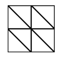
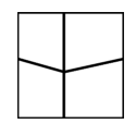
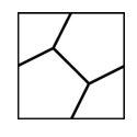
(a) Initial level ${\mathcal{L}}=1$, fine level $\ell=0$

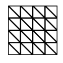
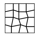
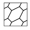
(b) Initial level ${\mathcal{L}}=2$, fine level $\ell=0$

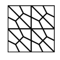
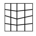
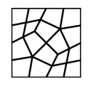
(c) Initial level ${\mathcal{L}}=1$, fine level $\ell=1$

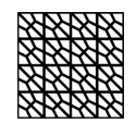
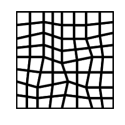
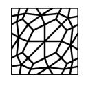
(d) Initial level ${\mathcal{L}}=2$, fine level $\ell=1$

Figure 3: Top: $Tria$, $Quad$ and $Hex$ meshes with initial levels ${\mathcal{L}}=1$ (left) and ${\mathcal{L}}=2$ (right) and fine level $\ell=0$. Bottom: corresponding grids obtained after a uniform refinement ($\ell=1$) employing the refinement strategy of Section 3.

As pre-smoother we employ $\nu$ steps of the Gauss-Seidel iterative algorithm, while a direct solver is employed to solve the coarse problem. All simulations are performed by using the null vector as initial guess, and we use as stopping criterium $\|{\bm{r}}^{(k)}\|\leq 10^{-9}\|{\bm{b}}\|$, being ${\bm{r}}^{(k)}$ the residual at the $k$-th iteration, ${\bm{b}}$ the right-hand side of the linear system, and $\|\cdot\|$ the Euclidean norm.

	it.	$\rho$	${\mathcal{K}}(\bm{A})$	rate	it.	$\rho$	${\mathcal{K}}(\bm{A})$	rate	it.	$\rho$	${\mathcal{K}}(\bm{A})$	rate
$\ell=1$	18	0.3	1.1e+1	-	9	0.1	5.9e+0	-	7	0.1	6.9e+0	-
$\ell=2$	13	0.2	4.9e+1	2.2	8	0.1	2.6e+1	2.1	8	0.1	3.2e+1	2.2
$\ell=3$	18	0.1	2.2e+2	2.1	8	0.1	1.1e+2	2.0	10	0.1	1.4e+2	2.1
$\ell=4$	22	0.4	9.2e+2	2.1	9	0.1	4.2e+2	2.0	11	0.1	6.2e+2	2.1
$\ell=5$	23	0.4	3.9e+3	2.0	9	0.1	1.7e+3	2.0	12	0.2	1.1e+4	2.1
	$Tria$ grids				$Quad$ grids				$Hex$ grids

Table 1: Iteration counts of the two-level algorithm and computed convergence factor $\rho$ for different fine refinement level $\ell$ starting from the initial grids of in Figure 3 with ${\mathcal{L}}=1$. For completeness, the condition number of the stifness matrix ${\mathcal{K}}(\bm{A})$ and its growth rate are also reported. Number of pre-smoothing steps $\nu=2$.

In Table 1 we report, starting from the initial grids shown in Figure 3 with $\ell=0$, and ${\mathcal{L}}=1$, the iteration counts of our two-level algorithm when varying the fine refinement level $\ell$. This set of experiments has been obtained with $\nu=2$ pre-smoothing steps. We clearly observe that our solver seems to be robust as the mesh size goes to zero: indeed the iteration counts are almost independent of the size of the problem. In Table 1 we also show the computed convergence factor

$$\rho=\textrm{exp}\left(\frac{1}{n}\log\frac{\|{\bm{r}}^{(n)}\|}{\|{\bm{r}}^{(0)}\|}\right),$$ (27)

where $n$ is the number of iterations needed to achieve convergence. Finally, for completeness, we have also computed the condition number of the stiffness matrix $\kappa(\bm{A})$ as well as its growth rate (cf. Table 1). As expected, we can clearly observe that the condition number increases quadratically as the mesh is refined.

	it.	$\rho$	${\mathcal{K}}(\bm{A})$	rate	it.	$\rho$	${\mathcal{K}}(\bm{A})$	rate	it.	$\rho$	${\mathcal{K}}(\bm{A})$	rate
$\ell=1$	16	0.3	4.3e+1	-	8	0.1	2.7e+1	-	7	0.1	1.3e+1	-
$\ell=2$	14	0.2	2.0e+1	2.2	9	0.1	1.1e+2	2.1	14	0.2	6.5e+1	2.4
$\ell=3$	17	0.2	8.6e+2	2.1	10	0.1	4.6e+2	2.0	18	0.3	3.3e+2	2.4
$\ell=4$	21	0.4	3.7e+3	2.1	10	0.1	1.9e+3	2.0	22	0.4	2.1e+3	2.6
	$Tria$ grids				$Quad$ grids				$Hex$ grids

Table 2: Iteration counts of the two-level algorithm and computed convergence factor $\rho$ for different fine refinement levels $\ell$ starting from the coarse grids of in Figure 3 with ${\mathcal{L}}=2$. For completeness, the condition number of the stifness matrix ${\mathcal{K}}(\bm{A})$ and its growth rate are also reported. Number of pre-smoothing steps $\nu=2$.

We have repeated the same set of experiments starting from the initial grids depicted in Figure 3 with ${\mathcal{L}}=2$ and $\ell=0$. The computed results are reported in Table 2. Notice that, in this case, on $Hex$-type grids the condition number seems to grows slightly faster than expected.

Next, we address the influence of the number of smoothing steps of the performance of our two-level solver. In Table  3 we report the iteration counts when increasing the number of pre-smoothing steps $\nu=3,4,5$. The results shown in Table 3 have been obtained starting from the initial grids of Figure 3 with ${\mathcal{L}}=1$ and $\ell=0$; the corresponding ones obtained with the initial grids of Figure 3, ${\mathcal{L}}=2$ and $\ell=0$ are completely analogous and are not reported here, for the sake of brevity. From the iteration counts reported in Table 3 we can conclude that (i) in all the cases considered, our two-level method is robust as the mesh size is refined; (ii) as expected, the performance of the algorithm improves as the number of smoothing steps increases.

	$\nu=3$	$\nu=4$	$\nu=5$	$\nu=3$	$\nu=4$	$\nu=5$	$\nu=3$	$\nu=4$	$\nu=5$
$\ell=1$	11	9	8	7	6	5	6	6	5
$\ell=2$	10	9	8	7	6	6	7	6	6
$\ell=3$	11	11	9	7	6	6	8	7	7
$\ell=4$	15	12	10	7	6	6	8	8	7
$\ell=5$	16	13	11	7	6	6	9	8	7
	$Tria$ grids			$Quad$ grids			$Hex$ grids

Table 3: Iteration counts as a function of the number of pre-smoothing steps $\nu=3,4,5$ and for different fine refinement levels $\ell$ starting from the initial grids of Figure 3, ${\mathcal{L}}=1$.

Finally, we demonstrate numerically that our scheme also provides a uniform preconditioner, that is the number of PCG iterations needed to achieve convergence up to a (user-defined) tolerance is uniformly bounded independently of the number of degrees of freedom whenever CG is accelerated by the preconditioner described in Section 3. In Table 4 we report the PCG iteration counts as a function of the number of the fine level $\ell=1,2,3,4,5$ starting from the initial grids shown in Figure 3 (${\mathcal{L}}=1,2$, $\ell=0$) for $Hex$-type grids. For completeness, we also report the computed convergence factor $\rho$ (second and fifth columns) and the correspondindg CG iteration counts needed to solve the unpreconditioned system (third and sixth columns). It is clear that employing our preconditioner leads to a uniformly bounded number of iterations (independent of the characteristic size of the underling partition). On the other hand, the iteration counts needed to solve the unpreconditioned systems grows linearly as the mesh size goes to zero.

	PCG it.	$\rho$	CG it.	PCG it.	$\rho$	CG it.
$\ell=1$	10	0.25	19	11	0.27	30
$\ell=2$	12	0.29	42	10	0.25	66
$\ell=3$	10	0.23	92	10	0.23	133
$\ell=4$	10	0.23	210	10	0.24	324
$\ell=5$	10	0.25	533	-	-	-
	${\mathcal{L}}=1$			${\mathcal{L}}=2$

Table 4: PCG iteration counts and computed convergence factor $\rho$ as a function of the number of level $\ell$ starting from the initial grids of Figure 3, ${\mathcal{L}}=1,2$, $Hex$ grids. For comparison, the CG iteration counts needed to solve the unpreconditioned systems are also reported.

5 Conclusions

We have proposed and analyzed a two level preconditioner for mimetic finite difference discretizations of elliptic equations. Our preconditioner use inexact coarse grid solver (non-inherited coarse grid bilinear form) and results in a optimal method with sparser coarse grid operators. We proved that the condition number of the preconditioned system is uniformly bounded. We also implemented the preconditioner and verified numerically the theoretical results.

6 Acknowledgements

Part of this work was completed while the third author was visiting MOX at Politecnico di Milano in 2013. Thanks go to the MOX for the hospitality and support. The work of the first and second author has been partially founded by the 2013 GNCS project “Aspetti emergenti nello studio di strategie adattative per problemi differenziali”. The research of the third author was supported in part by NSF DMS-1217142, NSF DMS-1418843, and Lawrence Livermore National Laboratory through subcontract B603526.

References

- [1] P. F. Antonietti, L. Beirão da Veiga, C. Lovadina, and M. Verani. Hierarchical a posteriori error estimators for the mimetic discretization of elliptic problems. SIAM J. Numer. Anal., 51(1):654–675, 2013.
- [2] P. F. Antonietti, L. Beirão da Veiga, and M. Verani. Numerical performance of an adaptive MFD method for the obstacle problem. In Numerical Mathematics and Advanced Applications. Proceedings of the 9th European Conference on Numerical Mathematics and Advanced Applications, Springer Verlag Italia. Springer, Berlin, 2013.
- [3] P. F. Antonietti, L. Beirão da Veiga, N. Bigoni, and M. Verani. Mimetic finite differences for nonlinear and control problems. Math. Models Methods Appl. Sci., 24(8):1457–1493, 2014.
- [4] P. F. Antonietti, L. Beirão da Veiga, and M. Verani. A mimetic discretization of elliptic obstacle problems. Math. Comp., 82(283):1379–1400, 2013.
- [5] P. F. Antonietti, N. Bigoni, and M. Verani. Mimetic discretizations of elliptic control problems. Journal of Scientific Computing, 56(1):14–27, 2013.
- [6] P. F. Antonietti, N. Bigoni, and M. Verani. Mimetic finite difference approximation of quasilinear elliptic problems. Calcolo, 2014. DOI: 10.1007/s10092-014-0107-y.
- [7] P. F. Antonietti, P. Houston, M. Sarti, and M. Verani. W-cycle multigrid algorithms for -version interior penalty discontinuous Galerkin methods on polygonal and polyhedral meshes. in preparation, 2014.
- [8] P. F. Antonietti, M. Sarti, and M. Verani. Multigrid algorithms for -discontinuous Galerkin discretizations of elliptic problems. MOX Report 61/2013, Politecnico di Milano. ArXiv:1310.6573v4. Submitted.
- [9] L. Beirão da Veiga. A residual based error estimator for the mimetic finite difference method. Numer. Math., 108(3):387–406, 2008.
- [10] L. Beirão da Veiga. A mimetic finite difference method for linear elasticity. M2AN Math. Model. Numer. Anal., 44(2):231–250, 2010.
- [11] L. Beirão da Veiga, J. Droniou, and G. Manzini. A unified approach to handle convection terms in mixed and hybrid finite volumes and mimetic finite difference methods, 2011. To appear on IMA J. Numer Anal.; published online.
- [12] L. Beirão da Veiga, V. Gyrya, K. Lipnikov, and G. Manzini. Mimetic finite difference method for the Stokes problem on polygonal meshes. J. Comput. Phys., 228(19):7215–7232, 2009.
- [13] L. Beirão da Veiga and K. Lipnikov. A mimetic discretization of the Stokes problem with selected edge bubbles. SIAM J. Sci. Comp., 32(2):875–893, 2010.
- [14] L. Beirão da Veiga, K. Lipnikov, and G. Manzini. Convergence of the mimetic finite difference method for the Stokes problem on polyhedral meshes. SIAM J. Numer. Anal., 48(4):1419–1443, 2010.
- [15] L. Beirão da Veiga, K. Lipnikov, and G. Manzini. Arbitrary-order nodal mimetic discretizations of elliptic problems on polygonal meshes. SIAM J. Numer. Anal., 49:1737–1760, 2011.
- [16] L. Beirão da Veiga, K. Lipnikov, and G. Manzini. Arbitrary order nodal mimetic discretizations of elliptic problems on polygonal meshes. SIAM J. Numer. Anal., 49:1737–1760, 2011.
- [17] L. Beirão da Veiga and G. Manzini. A higher-order formulation of the mimetic finite difference method. SIAM J. Sci. Comp., 31(1):732–760, 2008.
- [18] L. Beirão da Veiga, F. Brezzi, A. Cangiani, G. Manzini, L. D. Marini, and A. Russo. Basic principles of virtual element methods. Math. Models Methods Appl. Sci., 23(1):199–214, 2013.
- [19] L. Beirão da Veiga, F. Brezzi, and L. D. Marini. Virtual elements for linear elasticity problems. SIAM J. Numer. Anal., 51(2):794–812, 2013.
- [20] L. Beirão da Veiga and D. Mora. A mimetic discretization of the Reissner–Mindlin plate bending problem. Numer. Math., 117(3):425–462, 2011.
- [21] J. H. Bramble. Multigrid methods, volume 294 of Pitman Research Notes in Mathematics Series. Longman Scientific & Technical, Harlow, 1993.
- [22] F. Brezzi and A. Buffa. Innovative mimetic discretizations for electromagnetic problems. J. Comput. Appl. Math., 234(6):1980–1987, 2010.
- [23] F. Brezzi, A. Buffa, and K. Lipnikov. Mimetic finite differences for elliptic problems. M2AN Math. Model. Numer. Anal., 43(2):277–295, 2009.
- [24] F. Brezzi, A. Buffa, and K. Lipnikov. Mimetic finite differences for elliptic problems. M2AN Math. Model. Numer. Anal., 43(2):277–295, 2009.
- [25] F. Brezzi, K. Lipnikov, and M. Shashkov. Convergence of the mimetic finite difference method for diffusion problems on polyhedral meshes. SIAM J. Numer. Anal., 43(5):1872–1896, 2005.
- [26] F. Brezzi, K. Lipnikov, and M. Shashkov. Convergence of mimetic finite difference method for diffusion problems on polyhedral meshes with curved faces. Math. Models Methods Appl. Sci., 16(2):275–297, 2006.
- [27] F. Brezzi, K. Lipnikov, M. Shashkov, and V. Simoncini. A new discretization methodology for diffusion problems on generalized polyhedral meshes. Comput. Methods Appl. Mech. Engrg., 196(37-40):3682–3692, 2007.
- [28] F. Brezzi, K. Lipnikov, and V. Simoncini. A family of mimetic finite difference methods on polygonal and polyhedral meshes. Math. Models Methods Appl. Sci., 15(10):1533–1551, 2005.
- [29] F. Brezzi and L. D. Marini. Virtual element methods for plate bending problems. Comput. Methods Appl. Mech. Engrg., 253:455–462, 2013.
- [30] A. Cangiani, E. H. Georgoulis, and P. Houston. -version discontinuous Galerkin methods on polygonal and polyhedral meshes. Math. Models Methods Appl. Sci., 24(10):2009–2041, 2014.
- [31] A. Cangiani and G. Manzini. Flux reconstruction and pressure post-processing in mimetic finite difference methods. Comput. Methods Appl. Mech. Engrg., 197(9-12):933–945, 2008.
- [32] A. Cangiani, G. Manzini, and A. Russo. Convergence analysis of the mimetic finite difference method for elliptic problems. SIAM J. Numer. Anal., 47(4):2612–2637, 2009.
- [33] B. Chazelle. Convex partitions of polyhedra: a lower bound and worst-case optimal algorithm. SIAM J. Comput., 13(3):488–507, 1984.
- [34] J. Cheeger. A lower bound for the smallest eigenvalue of the Laplacian. In Problems in Analysis, pages 195–199. Princeton Univ. Press, 1970.
- [35] D. Cho, J. Xu, and L. Zikatanov. New estimates for the rate of convergence of the method of subspace corrections. Numer. Math. Theory Methods Appl., 1(1):44–56, 2008.
- [36] J. Dodziuk. Difference equations, isoperimetric inequality and transience of certain random walks. Transactions of the American Mathematical Society, 284:787–794, 1984.
- [37] W. Hackbusch. Multigrid methods and applications, volume 4 of Springer Series in Computational Mathematics. Springer-Verlag, Berlin, 1985.
- [38] R. Hiptmair and J. Xu. Nodal auxiliary space preconditioning in and spaces. SIAM J. Numer. Anal., 45(6):2483–2509 (electronic), 2007.
- [39] X. Hu, S. Wu, X.-H. Wu, J. Xu, C.-S. Zhang, S. Zhang, and L. Zikatanov. Combined Preconditioning with Applications in Reservoir Simulation. Multiscale Model. Simul., 11(2):507–521, 2013.
- [40] J. Hyman, M. Shashkov, and S. Steinberg. The numerical solution of diffusion problems in strongly heterogeneous non-isotropic materials. J. Comput. Phys., 132(1):130–148, 1997.
- [41] J. M. Hyman and M. Shashkov. Approximation of boundary conditions for mimetic finite-difference methods. Comput. Math. Appl., 36(5):79–99, 1998.
- [42] M. Jerrum and A. Sinclair. Approximating the permanent. SIAM J. Computing, 18:1149–1178, 1989.
- [43] J. K. Kraus. Algebraic multigrid based on computational molecules. II. Linear elasticity problems. SIAM J. Sci. Comput., 30(1):505–524, 2007/08.
- [44] J. K. Kraus, P. S. Vassilevski, and L. T. Zikatanov. Polynomial of best uniform approximation to 1/x and smoothing in two-level methods. Computational Methods in Applied Mathematics, 12(4):448—468, 2012.
- [45] I. Lashuk and P. S. Vassilevski. On some versions of the element agglomeration AMGe method. Numer. Linear Algebra Appl., 15(7):595–620, 2008.
- [46] I. V. Lashuk and P. S. Vassilevski. Element agglomeration coarse Raviart-Thomas spaces with improved approximation properties. Numer. Linear Algebra Appl., 19(2):414–426, 2012.
- [47] K. Lipnikov, G. Manzini, F. Brezzi, and A. Buffa. The mimetic finite difference method for the 3D magnetostatic field problems on polyhedral meshes. J. Comput. Phys., 230(2):305–328, 2011.
- [48] K. Lipnikov, J. Moulton, and D. Svyatskiy. A Multilevel Multiscale Mimetic (M3) method for two-phase flows in porous media. J. Comp. Phys., 227:6727–6753, 2008.
- [49] S. V. Nepomnyaschikh. Decomposition and fictitious domains methods for elliptic boundary value problems. In Fifth International Symposium on Domain Decomposition Methods for Partial Differential Equations (Norfolk, VA, 1991), pages 62–72. SIAM, Philadelphia, PA, 1992.
- [50] J. E. Pasciak and P. S. Vassilevski. Exact de Rham sequences of spaces defined on macro-elements in two and three spatial dimensions. SIAM J. Sci. Comput., 30(5):2427–2446, 2008.
- [51] P. S. Vassilevski. Multilevel block factorization preconditioners. Springer, New York, 2008. Matrix-based analysis and algorithms for solving finite element equations.
- [52] J. Xu. The auxiliary space method and optimal multigrid preconditioning techniques for unstructured grids. Computing, 56(3):215–235, 1996. International GAMM-Workshop on Multi-level Methods (Meisdorf, 1994).
- [53] L. T. Zikatanov. Two-sided bounds on the convergence rate of two-level methods. Numer. Linear Algebra Appl., 15(5):439–454, 2008.