A multiscale HDG method for second order elliptic equations.
Part I. Polynomial and homogenization-based multiscale spaces
Abstract
We introduce a finite element method for numerical upscaling of second order elliptic equations with highly heterogeneous coefficients. The method is based on a mixed formulation of the problem and the concepts of the domain decomposition and the hybrid discontinuous Galerkin methods. The method utilizes three different scales: (1) the scale of the partition of the domain of the problem, (2) the sale of partition of the boundaries of the subdomains (related to the corresponding space of Lagrange multipliers), and (3) the fine grid scale that is assumed to resolve the scale of the heterogeneous variation of the coefficients. Our proposed method gives a flexible framework that (1) couples independently generated multiscale basis functions in each coarse patch (2) provides a stable global coupling independent of local discretization, physical scales and contrast (3) allows avoiding any constraints (c.f., [8]) on coarse spaces. In this paper, we develop and study a multiscale HDG method that uses polynomial and homogenization-based multiscale spaces. These coarse spaces are designed for problems with scale separation. In our consequent paper, we plan to extend our flexible HDG framework to more challenging multiscale problems with non-separable scales and high contrast and consider enriched coarse spaces that use appropriate local spectral problems.
1 Introduction
In this paper we consider the following second order elliptic differential equation for the unknown function
| (1) |
with homogeneous Dirichlet boundary conditions. Here and are highly heterogeneous coefficients and is a bounded polyhedral domain in , . The presented in this paper methods are targeting applications of equation (1) to flows in porous media. Other possible applications are diffusion and transport of passive chemicals or heat transfer in heterogeneous media.
Flows in porous media appear in many industrial, scientific, engineering, and environmental applications. One common characteristic of these diverse areas is that porous media are intrinsically multiscale and typically display heterogeneities over a wide range of length-scales. Depending on the goals, solving the governing equations of flows in porous media might be sought at: (a) A coarse scale (e.g., if only the global pressure drop for a given flow rate is needed, and no other fine scale details of the solution are important), (b) A coarse scale enriched with some desirable fine scale details, and (c) The fine scale (if computationally affordable and practically desirable).
In naturally occurring materials, e.g. soil or rock, the permeability is small in granite formations (say cm2), medium in oil reservoirs, (say cm2 to cm2), and large in highly fractured or in vuggy media (say cm2). Numerical solution of such problems is a challenging task that has attracted a substantial attention in the scientific and engineering community.
In the last decade a number of numerical upscaling schemes that fall into the class of model reduction methods have been developed and used in various applications in geophysics and engineering related to problems in highly heterogeneous media. These include Galerkin multiscale finite element (e.g., [3, 13, 20, 18, 19]), mixed multiscale finite element (e.g., [1, 2, 5, 4]), the multiscale finite volume (see, e.g., [12, 23] mortar multiscale (see e.g., [8, 9], and variational multiscale (see e.g., [22]) methods. In the paper we present a general framework to design of numerical upscaling method based based on subgrid approximation using the hybrid discontinuous Galerkin finite element method (HDG) for second order elliptic equations. One of the earliest subgrid (variational multiscale) methods for Darcy’s problem in a mixed form have been developed by Arbogast in [3], see also [25].
In order to fix the main ideas and to derive the numerical upscaling method we shall consider model equation (1) with homogeneous Dirichlet boundary condition in a mixed form:
| (2a) | in , | ||||
| (2b) | in | ||||
| (2c) | on . | ||||
Here () is a bounded polyhedral domain, .
In the paper we present a multiscale finite element approximation of the mixed system (2a) – (2c) based on the hybridized discontinuous Galerkin method. Multiscale methods have gained substantial popularity in the last decade. We can consider them as a procedure of numerical upscaling that extends the capabilities of the mathematical theory of homogenization to more general cases including materials with non-periodic properties, non-separable scales, and/or random coefficients.
The first efficient mixed multiscale finite element methods were devised by Arbogast in [7] as multiblock grid approximations using the framework of mortaring technique. Mortaring techniques (e.g. see the pioneering work [10]) were introduced to accommodate methods that can be defined in separate subdomains that could have been independently meshed. This technique introduces an auxiliary space for a Lagrange multiplier associated with a continuity constraint on the approximate solution. The classical mortaring, devised for the needs of domain domain decomposition methods, has been adapted recently as multiscale finite element approximations, e.g. [4, 8, 9]. In a two-scale (two-grid, fine and coarse) method the aim is to resolve the local heterogeneities on the fine grid introduced on each coarse block and then ”glue” these approximations together via mortar spaces, that play the role of Lagrange multipliers, defined of the boundaries of the coarse partition. In order to design a stable method the mortar spaces have to satisfy proper inf-sup condition. This approach shown to be well suited for problems with heterogeneous media and a number of efficient methods and implementations have been proposed, studied, and used for solving a variety of applied problems, see, e.g. [3, 4, 6, 8].
The multiscale finite element method in this paper is based on discretization of the domain by using three different scales. First the domain is split into a number of non-overlapping subdomains with characteristic size . This partition, denoted by , represents a coarse scale at which the global features of the solution are captured, but the local features are not resolved. Each subdomain is partitioned into finite elements with size . This partition, denoted by , represents the scale at which the heterogeneities of the media are well represented and the local features of the solution can be resolved. Finally, on each interface of two adjacent subdomains from the partition we introduce an additional partition with characteristic size . This partition is used to introduce the space of the Lagrange multipliers, which will provide the means of gluing together of the fine-grid approximations that are introduced on each subdomain using the fine-grid partition . Three scales partition of the domains have been used in the mortar multiscale finite element methods by Arbogast and Xiao in [9], where the scale represents the size a cell at which a homogenized solution exits.
The hybridization of the finite element methods as outlined in [16] provides ample possibilities for ”gluing” together various finite element approximations. The mechanism of this ”glue” is based on the notion of numerical trace and numerical flux. Numerical trace is single valued function on the finite element interfaces and belongs to certain Lagrange multiplier space. This is also the space at which the global problem is formulated. The stability is ensured by a proper choice of the numerical flux, that involves a parameter , which proves stabilization of the scheme and some other desired properties (e.g. superconvergence) (for details, see, e.g. [15, 16, 17]). For multiscale methods, local basis functions are constructed independently in each coarse region. For this reason, approaches are needed that can flexibly couple these local multiscale local solutions without any constraints. In previous works, mortar multiscale methods are proposed to couple local basis functions; however, they require additional constraints on mortar spaces. The proposed approaches can avoid any constraints on coarse spaces and provide a flexible ”gluing” procedure for coupling multiscale basis functions. In this paper, we focus on polynomial and homogenization based multiscale spaces and study their stability and convergence properties.
The paper is organized as follows. In Sect. 2 we introduce the necessary notations and describe the multiscale FEM based on the framework of hybridizable discontinuous Galerkin method. In Subsection 2.4 we recast the two scale method into a hybridized form which essentially reduces to a symmetric and positive definite system for the Lagrange multipliers associated with the trace of the solution of the interfaces. In Section 2.5 we show that under reasonable assumptions on the finite dimensional spaces and the mesh, the two-scale method has unique solution.
In Section 3 we present the error analysis for the multiscale method. In Subsection 3.1 we introduce a number of projection operators related to the finite dimensional spaces (that are used later) and also a special projection operator related to the hybridizable discontinuous Galerkin FEM. Further, we state the approximation properties of these projections in terms of the scales of the various partitions of the domain. In Subsections 4.2 and 4.3 we derive error estimates for the flux and the pressure . Finally in Section 5, we study a new class of non-polynomial space for the numerical trace for special case of heterogeneous media with periodic arrangement of the coefficients. This space was proposed by Arbogast and Xiao [9] as a space for the mortar method for constructing multiscale finite element approximations and uses information of the local solution on the periodic cell. We show that the proposed multi-scale method is well posed and has proper approximation properties.
2 Multiscale Finite Element Method
Now we present the multiscale finite element approximation of the system (2a) – (2c). For this we shall need partition of the domain into finite elements, the corresponding finite elements spaces, and some notation from Sobolev spaces.
2.1 Sobolev spaces and their norms
Throughout the paper we shall use the standard notations for Sobolev spaces and their norm on the domain , subdomains or their boundaries. For example, , , , , , denote the Sobolev norms and semi-norms on and its boundary . For integer the Sobolev spaces are Hilbert spaces and the norms are defined by the -norms of their weak derivatives up to order . For non integer the spaces are defined by interpolation [21]. For instead of we shall use .
Further, we shall use various inequalities between norms and semi-norms related to embedding of Sobolev spaces. If and then we have the following inequalities:
| (3) |
We remark that since in this paper we are using three different scales () of partition of the domain we shall use these inequalities for domains of sizes or .
2.2 Partition of the domain
The finite element spaces that are used in the proposed method are defined below. They involve three different meshes. Let be a disjoint polygonal partition of the domain which allows nonconforming decomposition, see e.g. Figure 1, and let the maximal diameter of all be . Let be quasi-uniform conforming triangulations of with maximum element diameter , denote by , and let . Let denote the set of all edges/faces of the triangulation and . We also set . Consistently in this paper we shall denote by the subdomains of the partition while by we shall denoted the finite elements of the fine partition .
We call a interface of the partition if is either shared by two neighboring subdomains, or . For each interface , let be a quasi-uniform partition of with maximum element diameter . Set and
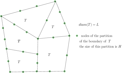
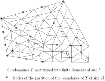
Thus, we have three scales: (1) – the maximum size of the of the subdomains , (2) – the size of the partition of the boundaries of , and finally (3) the scale of the fine-grid mesh – the maximum diameter of the finite elements introduced in each subdomain . In this paper we shall assume that the and .
Below is a summary of the above notation by grouping them into categories according to the scale they represent:
Note that the scale is associated only with the partition of the boundaries of the subdomains of the partition .
2.3 Multiscale FEM
The methods we are interested in seek an approximation to by the hybridized discontinuous Galerkin finite element method. For this purpose we need finite element spaces for these quantities consisting of piece-wise polynomial functions. Namely, we introduce
| where the spaces are defined as | ||||
Now the hybridizable multicsale DG FEM reads as follows: find in the space that satisfies the following weak problem
| (4a) | ||||||
| (4b) | ||||||
| (4c) | ||||||
| (4d) | ||||||
Since by the requirement the last equation is trivially satisfied and therefore it is redundant. However, we prefer to have it written explicitly for later use in the error analysis.
For , we write , where denotes the integral of over the domain . We also write where denotes the integral of over the boundary of the domain . The definition of the method is completed with the definition of the normal component of the numerical trace:
| (5) |
On each , the stabilization parameter is non-negative constant on each and we assume that on at least one face . By taking particular choices of the local spaces , and , and the linear local stabilization operator , various mixed () and HDG () methods are obtained. For a number of such choices we refer to [16, 17]. We note that on each fine element the local spaces can be any set of the spaces presented in [17, Tables 1 – 9]. It could be any classical mixed elements or the HDG elements defined on different triangulations. In Table 1 we give examples of local spaces for the classical mixed element and HDG element defined on a simplex.
| method | ||||
|---|---|---|---|---|
One feature of our formulation is that the choice of the space is totally free. In this paper, we will consider two different choices. The first choice is the space of piece-wise polynomials defined in (12), while the second is the space uses multiscale functions defined in (34). In general it can consist of any function spaces.
2.4 The upscaled structure of the method
The main feature of this method is that it could be implemented in such a way that we need to solve certain global system on the coarse mesh only. To show this possibility, we split (4c) into two equations by testing separately with and so that
| (6) |
Here . On any subdomain , given the boundary data of for , we can solve for by restricting the equations (4a)–(4c) on this particular :
for all . In fact the above local system is the regular HDG methods defined on . From [17] we already know that this system is stable. Hence, this HDG solver defines a global affine mapping from to . The solution can be further split into two parts, namely,
where satisfies
for all and satisfies
for all .
Then the second equation (6) reduces to
| (7) |
where the bilinear form and the linear form are defined as
| (8) |
Remark 1.
The same procedure can be applied also for the case of non-homogeneous data on . However, the presentation of this case is much more cumbersome. In order to simplify the notations and to highlight the main features of this method we have assumed homogeneous Dirichlet boundary data.
2.5 Existence of the solution of the FEM
The framework is general in terms of flexibility in the choice of the local spaces. However, in order to ensure the solvability of the system, we need some assumptions.
Assumption 2.
For any , an arbitrary face of , and , there exists a element such that
| for all , | ||||
| for all . |
This assumption is trivially satisfied by all classical mixed finite elements, e.g. RT, BDM, BDDF, etc. For these elements one can simply define , where is any solution of the problem:
where is the Fortin projection to the mixed elements (see, e.g. [11]). For the case of simplex triangulations and HDG elements, we refer the reader to [15, Lemma 3.2]. The proof for other HDG elements are very similar to the case of simplicial elements considered in [15].
Further, we need an assumption on the stabilization parameter :
Assumption 3.
On each , for any adjacent to , i.e. , there exists at least one element adjacent to , such that the stabilization operator on .
We are now ready to show the solvability of the method.
Theorem 4.
Proof.
Notice that the system (4) is a square system. It suffices to show that the homogeneous system has only the trivial solution. From (4d) we see that on . Now assume that is any solution of (4). Setting in (4a)-(4c) and adding all equations, we get after some algebraic manipulation,
By the definition of the numerical traces (5), we have
and since we get
| (9) |
and (4a) becomes
Now we take this over an element and after integration by parts we get
| (10) |
Since on than the second equality (9) implies that Next, by Assumption 2, there is such that
| for all , | ||||
| for all . |
where for , is the local orthogonal projection onto , for all . Inserting such in (10), we get
This implies that on . Since on , we get
| (11) |
Moreover, this means that for all . Taking , we have is piecewise constant on each . The above equation shows that on . On each , is a conforming triangulation, so this implies that for any interior face shared by two neighboring elements , the local spaces satisfy and hence coincides from both sides. This implies that in fact in each subdomain and .
In [8], in order to ensure the solvability of the mortar methods, the key assumption (roughly speaking) is that on the fine scale space should be rich enough comparing with the coarse scale space . In this paper, since the stabilization is achieved by the parameter we prove stability under the assumption that on each the parameter is strictly positive on some portion of . We do not need any conditions between the local spaces and .
3 Error Analysis
In this section we derive error estimates for the proposed above method. We would like stress on two important points of this method. First, in the most general case we have three different scales in our partitioning. The error estimates should reflect this generality of the setting. Second, upon different choices of the spaces and the stabilization strategy (i.e. the choice of the parameter ) we can get different convergence rates. For example, to obtain error estimates of optimal order we have to make some additional assumptions. All these are discussed in this section. For the sake of simplicity, we assume that the nonzero stabilization parameter is constant on all element In this section and the one follows, we only consider the method with the coarse space defined by polynomials, that is:
| (12) |
3.1 Preliminary Results
We present the main results in this section. In order to carry out a priori error estimates, we need some additional assumptions on the scheme. The first assumption is identical to Assumption A in [17], in order to be self-consistent, we still present it here:
Assumption 5.
The local spaces satisfy the following inclusion property:
| (13a) | ||||
| (13b) | ||||
On each element , there exist local projection operators
associated with the spaces , , defined by:
| (14a) | for all , | ||||
| (14b) | for all , | ||||
| (14c) | for all . | ||||
Assumption 6.
On each fine element , the stabilization operator is strictly positive on only one face .
Assumption 7.
For any element adjacent to the skeleton on a face , shared by and , is strictly positive, i.e. .
The above suggested local spaces or any set of local spaces presented in [17] satisfy Assumption 5. Moreover, assumptions 6 and 7 are the key to obtain optimal approximation results. In fact, without these two assumptions, we can still get some error estimates. However, the result will have a term with negative power of which is not desirable since is the finest scale. We will discuss this issue at the end of Section 4.2.
As a consequence of Assumption 6 and 7, the triangulation of each subdomain has to satisfy the requirement that each fine scale finite element can share at most one face with the coarse skeleton . This requirement implies that we need to put at least two fine elements to fill a corner of any subdomain. This suggests that we should use triangular (2D) or tetrahedral (3D) elements. In what follows, we restrict the choice of local spaces to be in Table 1. Notice that here we exclude the famous space from the table. Roughly speaking, the reason is that in the case of element, the local space is too small to provide a key property for the optimality of the error bound, see Lemma 15.
In [17] it has been shown that for any , the projection exists and is unique. Moreover, for all elements listed in Table 1, the projection has the following approximation property:
Lemma 8.
If the local spaces are mixed element spaces or , then
and if the local spaces are spaces, then
for all .
Further in our analysis we shall need some auxiliary projections and their properties:
| (15) |
where is the subset of of continuous functions and the Lagrange (nodal) interpolation operator.
In the analysis, we will need the following useful approximation properties of the projections , and the interpolation operator :
Lemma 9.
For any and any smooth enough function we have
| (17) | |||||
| (18) | |||||
| (19) |
Here the constant solely depends on the shape of the domain but not if its size.
Remark 10.
The regularity assumptions can be weakened to for any without reducing the approximation order. However, the above estimates make the presentation more transparent and shorter.
Proof.
(of Lemma 9) First we note the following standard estimates for the error on any edge/face , see [14]:
| (20a) | integer, | |||||
| (20b) | integer, | |||||
| (20c) | integer, | |||||
| (20d) | integer, | |||||
All three inequalities can be obtained by a similar scaling argument. Here we only present the proof of the first one of them. Assume is one of the faces of the element . By (20a), we have
for all integer . The case of non integer follows by interpolation and the other two are proven in a similar way. We note that the factor related to the scale of the subdomains . If the size of is then these estimates are well known. ∎
3.2 Main Result
We are now ready to state two main results for the methods, which proofs will postponed until Section 4. First we present the estimate for the vector variable the the weighted norm
Theorem 12.
Next we state the result regarding the error . It is valid under a typical elliptic regularity property we state next. Let is the solution of the dual problem:
| (21a) | in , | ||||
| (21b) | in , | ||||
| (21c) | on . | ||||
We assume that we have full regularity,
| (22) |
where only depends on the domain .
Theorem 13.
The above two results are based on a general framework which utilizes three different scales and a stabilization parameter . The richness of the proposed setup gives a flexibility that allows us to modify the method to fit different scenarios. On the other hand, it is hard to see the convergent rates of the methods based on this general setup. Now we discuss the results in details under some practical conditions. Here will simply assume the the coefficient is uniformly bounded.
Case 1: . Basically, this means that the subdomains have the same scale as the original domain . In this case, if we take , by the above two theorems and Lemma 8, we may summarize the order of convergence as follows:
In this case, our method is very close to the mortar methods introduced in [8]. Indeed, the mortar methods have the following convergence rate:
We can see that both methods have exactly the same order of convergence for . For the unknown , the HDG methods have an extra term . This suggests that HDG method little weaker approximation property if . This is due to the stabilization operator in the formulation. However, the advantage of the stabilization is that we don’t need any assumption between the spaces and .
If we choose , then the constant , combining Lemma 8, Theorem 12, 13, we obtain the following convergence rate:
We can see that in this situation, the convergence rates for both and are slightly degenerated.
Case 2: . From the practical point of view, this assumption suggests that we don’t further divide the edges of the subdomains . In this case, we also present the convergence rates by taking , respectively.
For , the order of convergence is:
For , the order of convergence is:
Similar as in Case 1, the convergence rates for both unknowns are worse if we choose .
We can see that if we choose the stabilization parameter inappropriately, the numerical solution does not even converge. On the other hand, if all other parameters are pre-assigned, we can follow a simple calculation to determine the optimal value of for the methods. We will illustrate this strategy with following setting: we assume that the polynomial degrees are given, , , the local spaces are HDG spaces. Then the order of convergence for solely depends on . Namely, it can be written as Applying the relation and setting , we obtain: where will be the minimum of the , and The above function is continuous with respect to . It is obvious that if . Therefore the absolute maximum of appears in the interval . Assume that achieves its maximum at , we can take to get optimal convergence rate for . This strategy can be applied to as well.
4 Proof of the main results
Now we prove the main results of the paper stated in Theorems 12 and 13. The proofs follow the technique developed in [17] for the hybridizable discontinuous Galerkin method and is done in several steps, by establishing first an estimate for the vector variable and then for scalar variable .
4.1 Error equations
We begin by obtaining the error equations we shall use in the analysis. The main idea is to work with the following projection errors:
| Further, we define | ||||
Lemma 14.
Under the Assumption 5, we have
| (23a) | |||||
| (23b) | |||||
| (23c) | |||||
| (23d) | |||||
for all . Here is the identity operator. Moreover,
| (24) |
Proof.
Let us begin by noting that the exact solution obviously satisfies
for all . By the orthogonality properties (14a) and (14b) of the projection , we obtain that
for all . Moreover, since is the -projection into , we get,
for all . Subtracting the four equations defining the weak formulation of the HDG method (4) from the above equations, respectively, we obtain the equations for the projection of the errors. The last error equation (23d) is due to the definition of on .
4.2 Estimate for
For the error estimate of we need to following lemma:
Proof.
Now take any . To prove that is -conforming in , we need to show that is continuous across all interior interfaces . By the error equation (23c), we know that is single valued on all interior interfaces due to the fact that and the test function are in the same space . Hence, it is suffices to show that
First of all, on each interior face , together with (24), we have
| (25) |
From here we can see that if . We only need to show that
| (26) |
On any adjacent with , by our assumptions, on where is on the boundary of . So on the other faces and hence .
Let us consider an arbitrary interior element with on . We restrict the error equation (23b) on , integrating by parts, we have
By (25) and the fact that on , we have
Since only on , we have
Now let be such that
| (27a) | |||||
| (27b) | |||||
One can easily see that such exists and is unique. Indeed, this is a square system for the coefficients of the polynomial and it is sufficient to show that the homogeneous system has only a trivial solution. On the equation represents a square homogeneous system for the trace . This ensures that the trace is identically zero on . Without loss of generality we can assume that is in the hyperplane . Then obviously with and now for all implies . Then we plug into the above error equation and notice that to get
This implies
and hence, for all . Consequently, for all .
To finish, we still need to show that when is adjacent with the boundary of . Similarly as interior element , error equation (23b) gives
Take to be again the unique element in such that
The second equation implies that on , so we have
This completes the proof. ∎
Remark 16.
The above proof cannot be applied for . Namely, a key step is the special choice of which satisfies (27). In the case of , is in a smaller space , hence the existence of is no longer valid.
We are now ready to obtain an upper bound of the -norm of . We first prove the following Lemma.
Lemma 17.
Proof.
By the error equation (23d) we know that . Taking in the error equations (23a)-(23c) respectively and adding, we get, after some algebraic manipulation,
Inserting the identity (24) in the above equation, we get
| Now using the fact that is single valued on and on we get | ||||
Finally noticing that on each
we get the identity
which completes the proof. ∎
Now we are ready to present our first estimate for :
Theorem 18.
Proof.
As a consequence, by triangle inequality, we immediately have the estimate for :
for .
From this estimate we see that we may have various scenarios in choosing the scales and and the stabilization parameter . Some of these were discussed in Subsection 3.2 For example, we take and assume , then has the order as , which is the same as the result in [8].
Remark 19.
It important to note that the fact that is essential in obtaining an optimal order of convergence. If were not -conforming, then we will have convergence rate . In the proof, -conformity of the vector field depends essentially on the fact that is single faced. It will be interesting to see what kind of numerical result we have if this assumption is failed.
4.3 Estimate for
Using a standard elliptic duality argument, we have the following result:
Lemma 20.
We have
| (28) |
where
Proof.
We begin by using the second equation (21b) of the dual problem to write that
by the first equation (21a) of the dual problem. This implies that
Taking in the first error equation, (23a), and in the second, (23b), we obtain
and, after simple algebraic manipulations we get
| (29) |
where
| Integrating by parts for the last two terms and applying the projection properties (14a), (14b) we have, | ||||
where
We will estimate separately. First we transform by adding and subtracting the terms and to get
Then using the identity , a simple consequence of the projection property (16), and error equation (24) we get
Next, we transform the expression by taking into account that and using the fact that for any :
Now combining and using the property (16) of the projections and , we get
To obtain the final estimate, on each interior face , and , by (23c), we note that is single valued on . Then we rewrite the last term as follows:
where is a Lagrange interpolant defined in (15). At the final step we have used the error equation (23c) and the fact that
Inserting the above expression into , we finally obtain:
which completes the proof. ∎
Notice that in Lemma 20 we established bounds for the projection errors: , and However, here we cannot apply the trace estimates of Lemma 9 for these terms since the solution of the dual problem is only in . Alternatively, we will bound these terms based on the following result:
Lemma 21.
If the function , then we have
| (30a) | ||||
| (30b) | ||||
| (30c) | ||||
| (30d) | ||||
Proof.
For (30a), on each , let denotes the projection of onto the local space . We have
The trace inequality (30b) can be proven in a similar way.
To prove (30c), we proceed as follows: on each subdomain , based on the partition , we can generate a conforming shape-regular triangulation . Therefore, we can also extend the boundary interpolation to the whole domain , denoted by . We have
In the last step we’ve applied the same trace inequality (3) and the standard interpolation approximation property.
For the last inequality, by the definition of , we have:
This completes the proof. ∎
Now we are ready to establish the final estimate for .
Theorem 22.
Let the assumptions of Theorem 18 hold and, in addition, let the local space contain piecewise linear functions for any , i.e. . Then
for all .
Proof.
We will estimate the terms in the error-norm representation (28) separately. By taking as the average of for each we get
| by (22) | ||||
Next we consider the term . First using the fact that for all we transform the integrals over the boundaries of the elements of the fine mesh into integrals on the boundaries on the coarse mesh only:
| Further, using the approximation property (30a)-(30b) and the regularity assumption (22) we get | ||||
Now we consider . Using , the approximation properties (18), (30a), (30b), and regularity assumption (22) we get
for any .
Combining the estimates for – and grouping the similar terms we get
for all . ∎
5 Multiscale HDG methods
In this section, we will consider the problem involving multiscale features. Namely, let us assume that the permeability coefficient has two separated scales,
| (31) |
where is called the slowly varying variable and is called the fast varying variable. Under this assumption, the exact solution also has two scales. Therefore, the derivatives of also depends on the small scale . In fact, the exact solution asymptotically behaves ([24]) as
for all . Here and denote any -th partial derivative of and , respectively. Then, if we set the nonzero to be constant 1, by Theorem 12, the velocity error becomes:
For a multiscale finite element method, the relation between all scales should be . The above estimate is no longer valuable since . The error for also has similar problem. In fact, this is a typical drawback for methods using polynomials for both fine and coarse scales. If we look at the estimate carefully, we can see the trouble appears on the term only. The scale is solely associated with the coarse space . This suggests that we should define the space in a more appropriate way so that its approximation property is independent of the scale . This reasoning has been used by Arbogast and Xiao [9] to design a mortar multiscale finite element method that overcomes this deficiency of the standard muliscale method. Their construction is based on the idea of involving the three scales we have used in our considerations. However, instead of using mortar spaces to glue the approximations on the coarse grid, here we use the same mechanism that is provided by the hybridization of the discontinuous Galerkin method.
5.1 Homogenization results
In a very special case of periodic arrangement of the heterogeneous coefficient we propose to use non-polynomial spaces for the Lagrange multipliers that are based on the concept of existence of smooth solution of a homogenized problem and using the first order correction from the homogenization theory.
We first review some classical homogenization results. For more details, we refer readers to [24, 18]. We assume that is periodic in with the unite cell as its period. The homogenized problem is defined as
| (32a) | |||||
| (32b) | |||||
| (32c) | |||||
Here the homogenized tensor is defined as
Here are the periodic solutions of the following cell problems:
where is the standard unit vector in . Then for the first order corrector
with we have the following result:
Lemma 23.
If , then there is some constant independent of , such that
Moreover, if , then we have (e.g., [24])
5.2 A multiscale coarse space
Using the above basic results form homogenization of heterogeneous differential operators we shall design our multiscale method. As before, we introduce finite element partitioning of the domain. In this setting we assume that the partitions are such that
| (33) |
In this section we shall use the same polynomial spaces and as before. The difference will be in the choice of the coarse space . Here we shall follow the work of Arbogast and Xiao [9], where this construction was used for the mortar finite element method.
For each , let denotes a rectangular neighborhood of , we define the local space as
| (34) |
Notice that, the local space involves both, local cell solutions and polynomial space . Therefore, its dimension is larger than . Simple considerations show that its dimension will depend on the structure of and will between and .
The coarse space is then defined as:
On each , we define the following projection of on :
Here is defined on as the orthogonal -projection of into . It has the following standard approximation property for and :
for all . Also, for any function , we have the following two trace inequalities:
The above two inequalities can be obtained by a simple scaling argument. Combining the trace inequalities and the approximation property of the interpolation, we get the following estimates:
| (35a) | ||||
| (35b) | ||||
After summation over the faces these estimates produce the following bounds:
| (36a) | ||||
| (36b) | ||||
for all .
We have the following approximation result:
Lemma 24.
Let (31) hold and let the homogenized solution be sufficiently smooth, i.e. . Then for
Proof.
The bound is obvious, since is an orthogonal projection on . Then by the triangle inequality, we have
Now we estimate the two terms on the right hand side separately. By the trace inequality (3) and the approximation property of homogenized solution established in Lemma 23, we have
The second term is bounded by using the approximation property (36) in the following manner:
for . This completes the proof. ∎
We can prove a better estimate for smoother . To get such a result we need an additional assumption on the space :
Assumption 25.
The space has a subspace which provides an approximation of order for smooth and the restriction on is conforming over the coarse skeleton .
If this assumption holds, we can define the interpolation of to be:
where is the -interpolation of onto . Under this assumption, the interpolation has the same approximation property (36) as .
In order to improve our estimates, we will need the following approximation result,
Lemma 26.
Proof.
Similar as in the proof of Lemma 24, we begin by splitting the term as:
For the first term, we apply the Stokes’ Theorem:
| by Lemma 15, | ||||
| by Lemma 23. |
For the second term, by the definition of the interpolation , we have:
| due to Assumption 25, we have , so we can apply Stokes’ Theorem on both terms and obtain | ||||
here we used the fact that . Finally, under the assumption (31), we have the classic result: , see [24]. Applying these results and the approximation result (36), we have
which completes the proof. ∎
5.3 Estimate for
We are now ready to establish the following result.
Theorem 27.
Let the coefficient satisfy (31). Then there exists a constant , independent of and , such that
| (37) | ||||
for all .
Proof.
Further, using the approximation properties of and established in Lemma 9 we get
and bound the term using Lemma 24.
In a similar way we estimate :
Finally, for , if we simply apply Cauchy-Schwarz inequality and trace inequality, we will have a term of order . This estimate is not desirable since . To bound in a better way, we first rewrite it using the error equation (23c):
Then using the equation (24) we get
Now we estimate these three terms separately. Now recall that for by Lemma 15. Thus using divergence theorem we get
Now using the trace inequality (3) (for ) and (36) we get
For estimating we apply Cauchy-Schwarz and triangle inequalities
and then bound using Lemma 24. For , we have
Then we estimate the term by Lemma 24 and get (37) by combining the estimates for .
As a consequence of Theorem 27, we immediately obtain an estimate for :
5.4 Estimate for
In Section 3, we use a standard duality argument to get an a priori estimate for . It is based on the full regularity assumption (22) of the adjoint equation (21). When the permeability coefficient has two separated scales, the regularity assumption is no longer valid. Instead, we consider the following adjoint problem:
| (39a) | in , | ||||
| (39b) | in , | ||||
| (39c) | on . | ||||
We assume the above problem has full regularity:
| (40) |
where only depends on the domain .
We are ready to state the estimate for :
Theorem 29.
Proof.
We begin by the fact that
| Then integrating by parts on the second term and using the property (14b) we get | ||||
Taking in the error equation (23a), we have
Now using the fact that are single valued on , so after some algebraic manipulation, we obtain:
We now estimate the above three terms separately.
| so that after using the full regularity assumption (40) and Lemma 8, we get | ||||
In order to bound the other two terms, we need the following bound:
| (41) |
On each , we use to denote the Clément interpolation from into . Then we have
the last step is due to the regularity condition (40). We now estimate the other two terms. First, we have the equality
due to the fact that on and is single valued on . We apply Cauchy-Schwarz inequality to obtain:
Finally, consider any interior edge . If on , by the identity (26), we have
On the other hand, if on , by the definition of the projection (14c), we still have the above identity. This applies
by the estimate (41). The proof is complete by combining the above three estimates. ∎
As a consequence of Theorem 29, Theorem 27 and Lemma 24, we immediately have the following estimate for :
Corollary 30.
6 Conclusions
In this paper, we introduce a hybrid discontinuous Galerkin method for solving multiscale elliptic equations. This is a first paper in a serious of two papers. In the present paper, we consider polynomial and homogenization-based coarse-grid spaces and lay a foundation of hybrid discontinuous Galerkin methods for solving multiscale flow equations. Our method gives a framework that (1) couples independently generated multiscale basis functions in each coarse patch (2) provides a stable global coupling independent of local discretization, physical scales and contrast (3) allows avoiding any constraints on coarse spaces. Though the coarse spaces in the paper are designed for problems with scale separation, the above properties of our framework are important for extending the method to more challenging multiscale problems with non-separable scales and high contrast. This is a subject of the subsequent paper.
7 Acknowledgements
Y. Efendiev’s work is partially supported by the DOE and NSF (DMS 0934837 and DMS 0811180). R. Lazarov’s research was supported in parts by NSF (DMS-1016525).
This publication is based in part on work supported by Award No. KUS-C1-016-04, made by King Abdullah University of Science and Technology (KAUST).
References
- [1] J.E. Aarnes. On the use of a mixed multiscale finite element method for greater flexibility and increased speed or improved accuracy in reservoir simulation. SIAM J. Multiscale Modeling and Simulation, 2:421–439, 2004.
- [2] J.E. Aarnes and Y. Efendiev. Mixed multiscale finite element for stochastic porous media flows. SIAM J. Sci. Comput., 30 (5):2319–2339, 2008.
- [3] T. Arbogast. Analysis of a two-scale, locally conservative subgrid upscaling for elliptic problems. SIAM J. Numer. Anal., 42(2):576–598 (electronic), 2004.
- [4] T. Arbogast. Homogenization-based mixed multiscale finite elements for problems with anisotropy. Multiscale Model. Simul., 9(2):624–653, 2011.
- [5] T. Arbogast and K.J. Boyd. Subgrid upscaling and mixed multiscale finite elements. SIAM J. Numer. Anal., 44(3):1150–1171 (electronic), 2006.
- [6] T. Arbogast and D.S. Brunson. A computational method for approximating a Darcy-Stokes system governing a vuggy porous medium. Comput. Geosci., 11(3):207–218, 2007.
- [7] T. Arbogast, L.C. Cowsar, M.F. Wheeler, and I. Yotov. Mixed finite element methods on nonmatching multiblock grids. SIAM J. Numer. Anal., 37(4):1295–1315, 2000.
- [8] T. Arbogast, G. Pencheva, M.F. Wheeler, and I. Yotov. A multiscale mortar mixed finite element method. Multiscale Model. Simul., 6(1):319–346, 2007.
- [9] T. Arbogast and H. Xiao. A miltiscale mortar mixed space based homogenization for heterogeneous elliptic problems. SIAM J. Numerical Analysis, 51 (1)(1):377–399, 2013.
- [10] C. Bernardi, Y. Maday, and A.T. Patera. Domain decomposition by the mortar element method. In HansG. Kaper, Marc Garbey, and GailW. Pieper, editors, Asymptotic and Numerical Methods for Partial Differential Equations with Critical Parameters, volume 384 of NATO ASI Series, pages 269–286. Springer Netherlands, 1993.
- [11] F. Brezzi and M. Fortin. Mixed and hybrid finite element methods, volume 15 of Springer Series in Computational Mathematics. Springer-Verlag, New York, 1991.
- [12] Y. Chen and L.J. Durlofsky. Adaptive local-global upscaling for general flow scenarios in heterogeneous formations. Transp. Porous Media, 62(2):157–185, 2006.
- [13] C.-C. Chu, I. G. Graham, and T.-Y. Hou. A new multiscale finite element method for high-contrast elliptic interface problems. Math. Comp., 79(272):1915–1955, 2010.
- [14] P. G. Ciarlet. The finite element method for elliptic problems. Elsevier North-Holland, New York, 1978.
- [15] B. Cockburn, B. Dong, and J. Guzmán. A superconvergent LDG-hybridizable Galerkin method for second-order elliptic problems. Math. Comp., 77(264):1887–1916, 2008.
- [16] B. Cockburn, J. Gopalakrishnan, and R. Lazarov. Unified hybridization of discontinuous Galerkin, mixed, and continuous Galerkin methods for second order elliptic problems. SIAM J. Numer. Analysis, 47(2):1319–1365, 2009.
- [17] B. Cockburn, W. Qiu, and K. Shi. Conditions for superconvergence of HDG methods for second-order elliptic problems. Math. Comp., 81(279):1327–1353, 2012.
- [18] Y. Efendiev and T.-Y. Hou. Multiscale Finite element Method. Springer-Verlag, Berlin, 2012.
- [19] Y.R. Efendiev, T.Y. Hou, and X.-H. Wu. Convergence of a nonconforming multiscale finite element method. Siam J. Numer. Anal., 37(3):888–910, 2000.
- [20] B. Engquist and Weinan E. The heterogeneous multi-scale methods. Commun. Math. Sci., 1:87–132, 2003.
- [21] P. Grisvard. Elliptic problems in nonsmooth domains. Pitman, Boston, MA, 1985.
- [22] T. Hughes, G. Feijoo, L. Mazzei, and J. Quincy. The variational multiscale method - a paradigm for computational mechanics. Comput. Methods Appl. Mech. Engrg., 166:3–24, 1998.
- [23] P. Jenny, S.H. Lee, and H. Tchelepi. Multi-scale finite volume method for elliptic problems in subsurface flow simulation. J. Comput. Phys., 187:47–67, 2003.
- [24] V.V. Jikov, S.M. Kozlov, and O.A. Oleinik. Homogenization of Differential Operators and Integral Functionals. Springer, 1st edition, 1994.
- [25] J. Nolen, G. Papanicolaou, and O. Pironneau. A framework for adaptive multiscale methods for elliptic problems. Multiscale Model. Simul., 7(1):171–196, 2008.