Three-Dimensional Radiation-Hydrodynamics Calculations of the Envelopes of Young Planets Embedded in Protoplanetary Disks

Abstract

We perform global three-dimensional (3D) radiation-hydrodynamics calculations of the envelopes surrounding young planetary cores of $5$, $10$, and $15$ Earth masses, located in a protoplanetary disk at $5$ and $10\,\mbox{AU}$ from a solar-mass star. We apply a nested-grid technique to resolve the thermodynamics of the disk at the orbital-radius length scale and that of the envelope at the core-radius length scale. The gas is modeled as a solar mixture of molecular and atomic hydrogen, helium, and their ions. The equation of state accounts for both gas and radiation, and gas energy includes contributions from rotational and vibrational states of molecular hydrogen and from ionization of atomic species. Dust opacities are computed from first principles, applying the full Mie theory. One-dimensional (1D) calculations of planet formation are used to supplement the 3D calculations by providing energy deposition rates in the envelope due to solids accretion. We compare 1D and 3D envelopes and find that masses and gas accretion rates agree within factors of $2$, and so do envelope temperatures. The trajectories of passive tracers are used to define the size of 3D envelopes, resulting in radii much smaller than the Hill radius and smaller than the Bondi radius. The moments of inertia and angular momentum of the envelopes are determined and the rotation rates are derived from the rigid-body approximation, resulting in slow bulk rotation. We find that the polar flattening is $\lesssim 0.05$. The dynamics of the accretion flow is examined by tracking the motion of tracers that move into the envelope. The anisotropy of this flow is characterized in terms of both its origin and impact site at the envelope surface. Gas merges with the envelope preferentially at mid- to high latitudes.

1. Introduction

The formation of a gaseous envelope around a planetary core has been studied, for over thirty years, by means of spherically symmetric one-dimensional (1D) calculations (e.g., Pollack et al., 1996). Most of the current knowledge about the process relies on such calculations. At early stages, the growth rate of the envelope is controlled by its own cooling rate, up the point where envelope and core mass are about equal. Thereafter, the growth is much more rapid and proceeds through a phase of hydrodynamical collapse, limited exclusively by disk supply. To date, the million-year evolution that is required to grow a planetary embryo into a giant planet can only be modeled via 1D calculations.

A number of properties and physical effects, however, cannot be accounted for or described by invoking spherical symmetry and are therefore approximated, imposed, or simply neglected in 1D models. The envelope radius, for example, can only be introduced as a parameter, since it depends on the thermal and gravitational energy of the gas outside the envelope (Bodenheimer & Pollack, 1986). The density and temperature at the outer boundary are approximated to average values in the unperturbed disk, whereas the actual (perturbed) disk values depend also on the planet mass. Rotation, often neglected, can be included to some extent, but not constrained. Although the gas dynamics of a disk away from a planet can be characterized as plane-parallel reasonably well, the flow becomes inherently three-dimensional (3D) as it approaches the planet (D’Angelo et al., 2003b; Bate et al., 2003; Masset et al., 2006). Part of this flow eventually feeds the envelope and breaks the spherical symmetry of the outer layers through transfer of angular and radial momentum, which may induce rotation and radial mixing.

3D models of envelopes that account for the interactions of the planet with the disk can in principle overcome all the limitations of 1D models. However, the computational overhead is so large that it is not yet feasible to go beyond evolution times of order $10^{2}$–$10^{3}$ years, depending on the orbital distance. At the moment, 3D calculations can only be used to investigate particular epochs of the core and envelope growth. Nonetheless, they can provide a wealth of information, otherwise not accessible through 1D models, which can help adjust and/or refine 1D calculations. The scope of this paper is to study one such epoch, early during the planet evolution when the accretion of solids is still relatively large and the envelope mass is much smaller than the core mass. We show that there is general consistency between 3D and 1D calculations and that 3D calculations can indeed address the physics missing in spherically symmetric models.

Local 3D calculations of planetary envelopes with radiation hydrodynamics were carried out by Ayliffe & Bate (2009, 2012). There are several similarities to our study but also important differences. For example, the local approach cannot capture the thermodynamics of the gas in and around the horse-shoe orbit region, which supplies the planet with gas and affects the dynamics of the accretion flow. They used an interstellar dust opacity, scaled down by numerical factors, whereas we compute the dust opacity based on a grain size distribution that may be more appropriate for circumstellar disks. They concentrated on somewhat larger core masses, and for the $10$ and $15$ Earth-mass ($M_{\mathrm{E}}$) cases they used core radii about $10$ times larger than the physical radii. They did not account for energy delivery by solids accretion. Recently, Nelson & Ruffert (2013) performed high-resolution, local calculations of the envelope region surrounding planetary cores of $10\,\mbox{$M_{\mathrm{E}}$}$, applying an isothermal and an adiabatic equation of state. The differences between the above-cited simulations and the calculations presented here are such as to render any comparison unfeasible. Until now, global 3D calculations of planets embedded in disks with radiation hydrodynamics have been used to investigate tidal torques exerted on the planet (e.g., Klahr & Kley, 2006; Paardekooper & Mellema, 2006; Kley et al., 2009), but never the details of the planet envelope and of the envelope-disk interactions.

The rest of the paper is organized as follows. The physical model, including equation of state and opacity, is described in Section 2, and various aspects of the numerical solution are outlined in Section 3. The thermodynamics of the equilibrium disk structures is discussed in Section 4, while the comparison with the 1D envelopes and the properties of the 3D envelopes are examined in Section 5. The conclusions are given in Section 6.

2. Disk and Envelope Thermodynamics

2.1. Gas Dynamics

Consider a frame of reference with its origin fixed to the star and rotating about the origin at a rate $\Omega$, the angular velocity of the planetary core around the star,

$$\Omega=\sqrt{\frac{G(\mbox{$M_{\star}$}+\mbox{$M_{c}$})}{a^{3}}},$$ (1)

where $M_{\star}$ is the stellar mass, $M_{c}$ indicates the core mass, and $a$ is the core’s semimajor axis. Equation (1) implicitly assumes that the envelope mass is small compared to $M_{c}$.

Consider now a spherical polar coordinate system $\{r,\theta,\phi\}$, where $r\in[a/2,2a]$ is the radial distance from the origin, $\theta\in[23\pi/50,\pi/2]$ is the meridional angle measured from the north pole (co-latitude), and $\phi\in[0,2\pi]$ is the azimuthal angle. Since the planet’s orbit lies in the disk’s equatorial plane ($\theta=\pi/2$), we assume that the disk is symmetric relative to this plane. The geometrical opening angle of the disk (above and below the equatorial plane) is $2\pi/25$, or about $14^{\circ}$.

As customary in many astrophysical applications, the disk’s gas is approximated as a viscous fluid with kinematic viscosity $\nu$, volume density $\rho$, and velocity $\boldsymbol{u}$. The dynamics of the gas is described via the mass continuity equation

$$\frac{\partial\rho}{\partial t}+\nabla\!\boldsymbol{\cdot}\!(\boldsymbol{u}\rho)=0$$ (2)

and the Navier-Stokes equations (see, e.g., Mihalas & Weibel Mihalas, 1999). Let us denote with $u_{r}$, $u_{\theta}$, and $u_{\phi}$, the spherical polar components of the velocity vector $\boldsymbol{u}$, and let the quantities $H_{r}=\rho u_{r}$, $H_{\theta}=\rho u_{\theta}r$, and $H_{\phi}=\rho(u_{\phi}+\Omega r\sin{\theta})r\sin{\theta}$, be the absolute linear ($H_{r}$) and angular ($H_{\theta}$ and $H_{\phi}$) momenta of the gas per unit volume.

By transformation and substitution, the Navier-Stokes equations can be re-written in the following conservative form in terms of absolute linear and angular momenta

$$\frac{\partial H_{r}}{\partial t}+\nabla\!\boldsymbol{\cdot}\!(\boldsymbol{u}H_{r}) = \frac{\rho}{r}\left[\left(\frac{H_{\theta}}{r}\right)^{2}+\left(\frac{H_{\phi}}{r\sin{\theta}}\right)^{2}\right]$$ (3)

$$- \frac{\partial P_{\mathrm{gas}}}{\partial r}-\rho\frac{\partial\Phi}{\partial r}$$

$$+ \mathcal{V}_{r}+\frac{\rho\kappa}{c}F_{r},$$

$$\frac{\partial H_{\theta}}{\partial t}+\nabla\!\boldsymbol{\cdot}\!(\boldsymbol{u}H_{\theta}) = \rho\left(\frac{\cos{\theta}}{\sin{\theta}}\right)\left(\frac{H_{\phi}}{r\sin{\theta}}\right)^{2}$$ (4)

$$- \frac{\partial P_{\mathrm{gas}}}{\partial\theta}-\rho\frac{\partial\Phi}{\partial\theta}$$

$$+ r\mathcal{V}_{\theta}+\frac{\rho\kappa}{c}rF_{\theta},$$

$$\frac{\partial H_{\phi}}{\partial t}+\nabla\!\boldsymbol{\cdot}\!(\boldsymbol{u}H_{\phi}) = -\frac{\partial P_{\mathrm{gas}}}{\partial\phi}-\rho\frac{\partial\Phi}{\partial\phi}$$ (5)

$$+ r\sin{\theta}\mathcal{V}_{\phi}+\frac{\rho\kappa}{c}r\sin{\theta}F_{\phi}\,.$$

In the above equations, $P_{\mathrm{gas}}$ is the gas pressure, which we shall discuss in more detail below, and $\Phi$ is the gravitational potential in the disk

$$\Phi=\Phi_{c}-\frac{G\,\mbox{$M_{\star}$}}{r}+\frac{G\,\mbox{$M_{c}$}}{r_{c}^{3}}\,\boldsymbol{r}\!\boldsymbol{\cdot}\!\boldsymbol{r}_{c},$$ (6)

in which $\Phi_{c}$ is the potential of the planetary core and $\boldsymbol{r}_{c}$ is the vector position of its center. We use a piecewise polynomial representation of the core’s potential, explicitly given in Appendix D, and assume that any gas bound to the core has a mass small compared to $M_{c}$. The third term on the right hand side of Equation (6) accounts for the fact that the reference frame is non-inertial since its origin is attached to the star.

The quantities $\mathcal{V}_{r}$, $\mathcal{V}_{\theta}$, and $\mathcal{V}_{\phi}$ in Equations (3), (4), and (5) represent the viscous force acting on a unit volume of gas. They depend on the components $\mathrm{S}_{ij}$ of the viscous stress tensor $\mathbf{S}$, which is assumed to be that of a Newtonian fluid without bulk viscosity. Explicit expressions for $\mathcal{V}_{r}$, $\mathcal{V}_{\theta}$, and $\mathcal{V}_{\phi}$ in spherical polar coordinates, along with those for the components $\mathrm{S}_{ij}$, are given in Mihalas & Weibel Mihalas (1999). Notice that Equations (4) and (5), which evolve angular momenta per unit volume, involve torques rather than forces. The last terms on the right-hand side of Equations (3), (4), and (5) are the forces/torques, per unit volume, imparted to the gas by the absorbed/scattered photons in the radiation field, of which $\boldsymbol{F}$ represents a frequency-integrated energy flux, $\kappa$ is a frequency-integrated opacity coefficient, and $c$ is the speed of light. As discussed below, we will identify $\kappa$ with the Rosseland mean opacity.

2.2. Gas Thermodynamics

Gas thermodynamics is considered under the approximation of local thermodynamic equilibrium and a single temperature, $T$, for the gas and the radiation. The radiation energy density is then written as $E_{\mathrm{rad}}=(4\pi/c)B(T)$, where $B(T)=(\sigma_{\mathrm{SB}}/\pi)T^{4}$ is the frequency-integrated Planck function and $\sigma_{\mathrm{SB}}$ is the Stefan-Boltzmann constant. Indicating with $E_{\mathrm{gas}}$ the gas energy density, the evolution of the gas and radiation energies are governed by (e.g., Turner & Stone, 2001)

$$\frac{\partial E_{\mathrm{gas}}}{\partial t}+\nabla\!\boldsymbol{\cdot}\!(\boldsymbol{u}E_{\mathrm{gas}})=-P_{\mathrm{gas}}\nabla\!\boldsymbol{\cdot}\!{\boldsymbol{u}}+\Psi+\varepsilon,$$ (7)

and

$$\frac{\partial E_{\mathrm{rad}}}{\partial t}+\nabla\!\boldsymbol{\cdot}\!(\boldsymbol{u}E_{\mathrm{rad}})=-\nabla\!\boldsymbol{\cdot}\!{\boldsymbol{F}}-P_{\mathrm{rad}}\nabla\!\boldsymbol{\cdot}\!{\boldsymbol{u}},$$ (8)

which here assume that the radiation pressure tensor is represented by a scalar matrix with scalar $P_{\mathrm{rad}}$. In a non-equilibrium situation, the right-hand sides of the above equations contain, respectively, the terms $\mp[4\pi\rho\kappa B(T)-c\rho\kappa E_{\mathrm{rad}}]$, which describe matter-radiation interaction but which vanish here on account of the assumed relation between $E_{\mathrm{rad}}$ and $B(T)$. Adding up Equations (7) and (8), the evolution equation of the total internal energy per unit volume, $E=E_{\mathrm{gas}}+E_{\mathrm{rad}}$, can be written as (e.g., Yorke & Kaisig, 1995)

$$\frac{\partial E}{\partial t}+\nabla\!\boldsymbol{\cdot}\!(\boldsymbol{u}E)=-\nabla\!\boldsymbol{\cdot}\!{\boldsymbol{F}}-P\nabla\!\boldsymbol{\cdot}\!{\boldsymbol{u}}+\Psi+\varepsilon.$$ (9)

In Equations (7) and (9), $\varepsilon V_{c}$ is the gravitational energy per unit time released by planetesimals penetrating the planet’s envelope, defined through the volume integral

$$\varepsilon V_{c}=\int{\frac{G\mbox{$M_{c}$}\dot{M}_{c}}{R_{c}}}\delta(\boldsymbol{r}-\boldsymbol{r}_{c})dV,$$ (10)

in which $V_{c}\sim(4\pi/3)R^{3}_{c}$ and $R_{c}$ is the core radius. The $\delta$-function is meant to signify that gravitational energy carried by planetesimals is released at the core surface. The accretion rate of the core, $\dot{M}_{c}$, and the core radius are input parameters discussed in Section 5.1.

The function $\Psi$, in Equations (7) and (9), accounts for viscous energy dissipation. In terms of the components of the viscous stress tensor, the dissipation function is (Mihalas & Weibel Mihalas, 1999).

$$\Psi=\frac{1}{2\nu\rho}\mathrm{S}_{ij}\mathrm{S}^{ij}=\frac{1}{2\nu\rho} \left(\mathrm{S}^{2}_{rr}+\mathrm{S}^{2}_{\theta\theta}+\mathrm{S}^{2}_{\phi\phi}+\right.$$ (11)

$$\left.2\mathrm{S}^{2}_{r\theta}+2\mathrm{S}^{2}_{r\phi}+2\mathrm{S}^{2}_{\theta\phi}\right).$$

The gas and radiation pressures are given by, respectively, $P_{\mathrm{gas}}=\rho k_{\mathrm{B}}T/(\mu m_{\mathrm{H}})$ and $P_{\mathrm{rad}}=E_{\mathrm{rad}}/3$. The mean molecular weight, $\mu$, accounts for the presence of molecules, atoms, and ions, and will be discussed in detail below ($k_{\mathrm{B}}$ is the Boltzmann constant and $m_{\mathrm{H}}$ is the atomic hydrogen mass). As mentioned earlier, the radiation pressure is a tensor whose components depend on the Eddington factor (e.g., Turner & Stone, 2001), although here we retain only the diagonal elements (assumed all equal) and use the general property that the trace of the tensor is equal to $E_{\mathrm{rad}}$ (Castor, 2007). This approximation works best for optically thick gas. In Equation (9), $P=P_{\mathrm{gas}}+P_{\mathrm{rad}}$ refers to the total pressure.

Energy transport via radiation is taken into account in the so-called flux-limited diffusion approximation (Levermore & Pomraning, 1981; Castor, 2007). The radiation energy flux is written as

$$\boldsymbol{F}=-\mathcal{D}\nabla{E_{\mathrm{rad}}}.$$ (12)

The flux-limited diffusion coefficient is

$$\mathcal{D}=\frac{c\lambda}{\rho\kappa},$$ (13)

in which the so-called flux-limiter, $\lambda$, is a function of the ratio $\mathcal{R}=|\nabla{E_{\mathrm{rad}}}|/(\rho\kappa E_{\mathrm{rad}})$. The choice of the flux-limiter is problem dependent (see discussion in Turner & Stone, 2001). In fact, there are only constraints in limiting cases. In the diffusion limit, i.e., for $\mathcal{R}\rightarrow 0$, $\lambda$ must tend to $1/3$, so that $\boldsymbol{F}=-c/(3\rho\kappa)\nabla{E_{\mathrm{rad}}}=-(16/3)\sigma_{\mathrm{SB}}/(\rho\kappa)T^{3}\nabla{T}$. In the streaming limit, i.e., for $\mathcal{R}\rightarrow\infty$, the asymptotic behavior must be $\lambda\rightarrow 1/\mathcal{R}$, so that $\boldsymbol{F}\rightarrow-\boldsymbol{n}cE_{\mathrm{rad}}$ with $\boldsymbol{n}=\nabla{E_{\mathrm{rad}}}/|\nabla{E_{\mathrm{rad}}}|$. Here, we adopt the rational approximation to the flux-limiter of Levermore & Pomraning (1981)

$$\lambda=\frac{2+\mathcal{R}}{6+3\mathcal{R}+\mathcal{R}^{2}}.$$ (14)

It should be mentioned that, as discussed by Castor (2007), regardless of the choice of the function $\lambda$, the flux-limited diffusion approximation can hardly describe the angular distribution of the radiation field to an accuracy better than $\sim 10$%.

The radiation flux in Equation (9) includes only radiation generated internally by the gas. However, the radiation flux from additional sources, such as irradiation by the star or other external sources, can be simply added to the flux in Equation (12), without any further modifications.

2.3. Equation of State

As anticipated above, we apply an equation of state for an ideal gas that accounts for the effects due to the dissociation of molecular hydrogen and of the ionization of atomic hydrogen and helium. Contributions from radiation are also taken into account. The mass fractions of hydrogen and helium are set equal, respectively, to $X=0.7$ and $Y=0.28$. These numbers deviate somewhat from current estimates of protosolar values, principally due to the availability of gas opacity tables, as discussed below. Asplund et al. (2009) and Lodders (2010) reported protosolar composition values of $X=0.71$ and $Y=0.27$. We neglect heavy elements in constructing the equation of state, although their contribution to gas opacity is taken into account (see Section 2.4).

Following Black & Bodenheimer (1975), let us introduce the degree of dissociation of molecular hydrogen, $y=\rho_{\mathrm{H}}/(\rho_{\mathrm{H}}+\rho_{\mathrm{H}_{2}})$, the degree of ionization of atomic hydrogen, $x=\rho_{\mathrm{H}^{+}}/(\rho_{\mathrm{H}^{+}}+\rho_{\mathrm{H}})$, and the degrees of single and double ionization of helium, $z_{1}=\rho_{\mathrm{He}^{+}}/(\rho_{\mathrm{He}^{+}}+\rho_{\mathrm{He}})$ and $z_{2}=\rho_{\mathrm{He}^{2+}}/(\rho_{\mathrm{He}^{2+}}+\rho_{\mathrm{He}^{+}})$, respectively. Applying the Saha equation (see Kippenhahn et al., 2013; Kowalski, 2006), the dissociation and ionization degrees can be derived from the following relations

$$\frac{y^{2}}{1-y} = \frac{m_{\mathrm{H}}}{2X\rho}\!\left(\frac{m_{\mathrm{H}}k_{\mathrm{B}}T}{4\pi\hbar^{2}}\right)^{3/2}e^{-4.48\mathrm{eV}/(k_{\mathrm{B}}T)}$$ (15)

$$\frac{x^{2}}{1-x} = \frac{m_{\mathrm{H}}}{X\rho}\!\left(\frac{m_{\mathrm{e}}k_{\mathrm{B}}T}{2\pi\hbar^{2}}\right)^{3/2}e^{-13.60\mathrm{eV}/(k_{\mathrm{B}}T)}$$ (16)

$$\frac{z_{1}}{1-z_{1}} = \frac{4m_{\mathrm{H}}}{\rho}\!\left(\frac{m_{\mathrm{e}}k_{\mathrm{B}}T}{2\pi\hbar^{2}}\right)^{3/2}\frac{e^{-24.59\mathrm{eV}/(k_{\mathrm{B}}T)}}{X+z_{1}Y/4}$$ (17)

$$\frac{z_{2}}{1-z_{2}} = \frac{m_{\mathrm{H}}}{\rho}\!\left(\frac{m_{\mathrm{e}}k_{\mathrm{B}}T}{2\pi\hbar^{2}}\right)^{3/2}\frac{e^{-54.42\mathrm{eV}/(k_{\mathrm{B}}T)}}{X+(z_{2}+1)Y/4},$$ (18)

where $m_{\mathrm{e}}$ is the electron mass and $\hbar$ is Planck’s constant divided by $2\pi$. The mean molecular weight, $\mu$, of the mixture is such that (e.g., Black & Bodenheimer, 1975; Kippenhahn et al., 2013)

$$\frac{\mu}{4}=[2X(1+y+2xy)+Y(1+z_{1}+z_{1}z_{2})]^{-1}.$$ (19)

The internal energy density of the mixture can be written as

$$E_{\mathrm{gas}} = \left(E_{\mathrm{H}_{2}}+E_{\mathrm{H}}+E_{\mathrm{He}}+E_{\mathrm{H+H}}+E_{\mathrm{H}^{+}}\right.$$ (20)

$$+ \left.E_{\mathrm{He}^{+}}+E_{\mathrm{He}^{2+}}\right)k_{\mathrm{B}}T\rho/m_{\mathrm{H}},$$

where all contributions in the parenthesis are dimensionless and all, except for the contribution of $\mathrm{H}_{2}$, are straightforward (see, e.g., Black & Bodenheimer, 1975): $E_{\mathrm{H}}=3X(1+x)y/2$, $E_{\mathrm{He}}=3Y(1+z_{1}+z_{1}z_{2})/8$, $E_{\mathrm{H+H}}=4.48\mathrm{eV}\,Xy/(2k_{\mathrm{B}}T)$, $E_{\mathrm{H}^{+}}=13.60\mathrm{eV}\,Xxy/(k_{\mathrm{B}}T)$, $E_{\mathrm{He}^{+}}=24.59\mathrm{eV}\,Yz_{1}(1-z_{2})/(4k_{\mathrm{B}}T)$, and $E_{\mathrm{He}^{2+}}=54.42\mathrm{eV}\,Yz_{1}z_{2}/(4k_{\mathrm{B}}T)$. The second and third terms in Equation (20) are the translational energies of hydrogen and helium atoms. The last four terms represent contributions due to dissociation of molecular hydrogen and ionization of atomic hydrogen and helium.

The energy of molecular hydrogen in Equation (20) takes into account, along with translational, also rotational and vibrational degrees of freedom (e.g., Pathria & Beale, 2011)

$$E_{\mathrm{H}_{2}}=\frac{X(1-y)}{2}\left[\frac{3}{2}+\frac{T}{\zeta_{v}}\frac{\partial\zeta_{v}}{\partial T}+\frac{T}{\zeta_{r}}\frac{\partial\zeta_{r}}{\partial T}\right],$$ (21)

in which $\zeta_{v}$ and $\zeta_{r}$ are the vibrational and rotational partition functions of the molecule, respectively.

The vibrational energy levels of a diatomic molecule can be described by the partition function of a quantum harmonic oscillator

$$\zeta_{v}=\left(1-e^{-\Theta_{v}/T}\right)^{-1},$$ (22)

with $\Theta_{v}=6140\,\mbox{$\mathrm{K}$}$ for the $\mathrm{H}_{2}$ molecule. The rotational energy levels must take into consideration the relative spin states of the two nuclei. Parahydrogen (anti-parallel spins) forms a singlet state, while orthohydrogen (parallel spins) forms an excited triplet state. At equilibrium, the percentage of the two forms depends on temperature. At temperatures $T\lesssim 50\,\mbox{$\mathrm{K}$}$, the parahydrogen singlet is the most populated energy state and more than $80$% of the molecules are in para-form. As the temperature rises, the orthohydrogen triplet state starts to be occupied. At temperatures $T\gtrsim 300\,\mbox{$\mathrm{K}$}$, all energy levels are equally populated, yielding an ortho-to-para ratio of $3/1$.

Approximating the rotational energy levels of $\mathrm{H}_{2}$ to those of a quantum rigid rotor, the rotational partition function of para/orthohydrogen can be expressed as

$$\zeta_{\mathrm{P,O}}=\sum_{j}\left(2j+1\right)e^{-j(j+1)\Theta_{r}/T}$$ (23)

with $\Theta_{r}=85.5\,\mbox{$\mathrm{K}$}$. The sum is performed over even integers for parahydrogen and over odd integers for orthohydrogen. Assuming equilibrium of the two forms at all temperatures and because of the spin degeneracy of the orthohydrogen triplet state, the total partition function is $\zeta_{r}=\zeta_{\mathrm{P}}+3\zeta_{\mathrm{O}}$ (e.g., Kittel, 2004; Pathria & Beale, 2011). However, conversion from one form to the other is quite inefficient in absence of a catalyst (e.g., Schmauch & Singleton, 1964), due to weak magnetic interaction of the nucleus spin with the outside world (e.g., Pathria & Beale, 2011; Draine, 2011).

Therefore, the two forms of $\mathrm{H}_{2}$ may be regarded as independent species (different molecules) with a given occurrence ratio $f_{\mathrm{O}}/f_{\mathrm{P}}$. In this case, the total partition function is the product of the single partition functions (e.g., Pathria & Beale, 2011)

$$\zeta_{r}=\zeta_{\mathrm{P}}^{f_{\mathrm{P}}}\left(\zeta_{\mathrm{O}}e^{2\Theta_{r}/T}\right)^{f_{\mathrm{O}}},$$ (24)

where $f_{\mathrm{O}}+f_{\mathrm{P}}=1$. Here we apply Equation (24) and assume a fixed number ratio $f_{\mathrm{O}}/f_{\mathrm{P}}=3$. As mentioned by Boley et al. (2007b), the exponential is meant to regularize $\zeta_{r}$ in the limit $T\rightarrow 0$. In this limit, $\zeta_{\mathrm{P}}\rightarrow 1$ and $\zeta_{\mathrm{O}}\rightarrow 0$ (recall that the triplet is an excited state), so that the requirement of a fixed number ratio would be violated.

By using Equations (24), (23) and (22), Equation (21) becomes

$$E_{\mathrm{H}_{2}} = \frac{X(1-y)}{2}\left[\frac{3}{2}+\left(\frac{\Theta_{v}}{T}\right)\frac{e^{-\Theta_{v}/T}}{1-e^{-\Theta_{v}/T}}\right.$$ (25)

$$+ \left.f_{\mathrm{P}}\frac{d\ln{\zeta_{\mathrm{P}}}}{d\ln{T}}+f_{\mathrm{O}}\left(\frac{d\ln{\zeta_{\mathrm{O}}}}{d\ln{T}}-\frac{2\Theta_{r}}{T}\right)\right].$$

As explained later, a stability condition for the numerical calculations requires an estimate of the adiabatic sound speed of the gas, $c_{\mathrm{gas}}=\sqrt{\Gamma_{1}P_{\mathrm{gas}}/\rho}$. The first adiabatic exponent, defined as $\Gamma_{1}=(\partial\ln{P_{\mathrm{gas}}}/\partial\ln{\rho})$ at constant entropy (Kippenhahn et al., 2013), can also be expressed as (Weiss et al., 2006)

$$\Gamma_{1}=\frac{1}{c_{V}}\left(\frac{P_{\mathrm{gas}}}{T\rho}\right)\chi^{2}_{T}+\chi_{\rho},$$ (26)

where the specific heat at constant volume, $c_{V}$, is calculated by taking the derivative with respect to $T$ of the specific energy of the gas $E_{\mathrm{gas}}/\rho$ (in Equation (20), $y$, $x$, $z_{1}$, and $z_{2}$ are all functions of $T$ and $\rho$), and the so-called temperature and density exponents, $\chi_{T}$ and $\chi_{\rho}$, are defined by

$$\chi_{T}=\left(\frac{\partial\ln{P_{\mathrm{gas}}}}{\partial\ln{T}}\right)_{\rho}=1-\frac{\partial\ln{\mu}}{\partial\ln{T}},$$ (27)

and

$$\chi_{\rho}=\left(\frac{\partial\ln{P_{\mathrm{gas}}}}{\partial\ln{\rho}}\right)_{T}=1-\frac{\partial\ln{\mu}}{\partial\ln{\rho}}.$$ (28)

All the summations required in the calculation of $\zeta_{\mathrm{P}}$, $\zeta_{\mathrm{O}}$, and their first and second derivatives with respect to $T$, use a sufficiently large number of terms so that the magnitude of the relative difference between the approximated and true sum is $\leq 10^{-8}$.

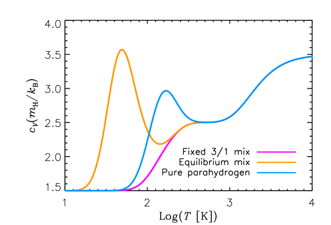
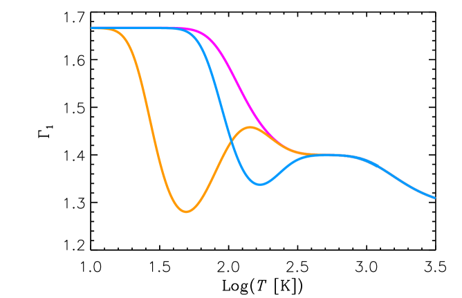
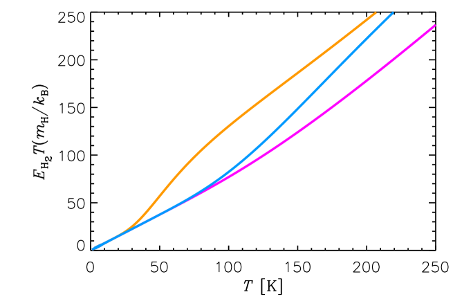
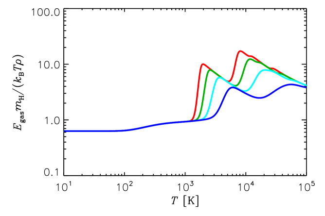
Figure 1.— Left: specific heat at constant volume (top), first adiabatic exponent (center) and specific energy times temperature (bottom) of molecular hydrogen. Note that both specific heat and specific energy are divided by $k_{\mathrm{B}}/m_{\mathrm{H}}$. The top and center panels are intended to reproduce Figures 1 and 2 of DeCampli et al. (1978), while the bottom panel replicates Figure 2 of Boley et al. (2007b). The different line styles refer, as indicated in the top panel, to a gas mixture with a fixed $1/3$ ratio between parahydrogen and orthohydrogen, a normal equilibrium mixture, and a parahydrogen gas. Right: same as for in the left panels, but for the actual gas mixture used in the calculations and four reference gas densities, as indicated in the top panel in units of $\mathrm{g\,cm^{-3}}$. The bottom panel shows the quantity in parenthesis on the right-hand side of Equation (20).

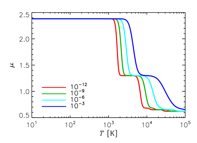
Figure 2.— Mean molecular weight, $\mu$, in Equation (19) for the gas mixture used in the calculations. Four reference values of the gas density $\rho$ are used, as indicated in the legend in units of $\mathrm{g\,cm^{-3}}$.

The left panels of Figure 1 show the specific heat (top), the first adiabatic exponent (center), and the specific energy (bottom) of $\mathrm{H}_{2}$ (see the figure caption for further details). The curves in the top and center panels should be compared to those in Figures 1 and 2 of DeCampli et al. (1978). The top panel also reproduces Figure 1 of Black & Bodenheimer (1975, there is a typo in their Equation (11), as the leading squared parenthesis of the second term should not be there). The curves in the bottom panel should be compared to the corresponding curves in Figure 2 of Boley et al. (2007b). The right panels of the figure show, for the actual gas mixture used in this work, the variation with temperature of $c_{V}=(\partial E_{\mathrm{gas}}/\partial T)_{\rho}$ divided by $k_{\mathrm{B}}/m_{\mathrm{H}}$ (top), $\Gamma_{1}$ in Equation (26) (center), and $E_{\mathrm{gas}}$ in Equation (20) divided by $k_{\mathrm{B}}T\rho/m_{\mathrm{H}}$ (bottom). The first adiabatic exponent of the actual gas mixture is basically constant below $\approx 50\,\mbox{$\mathrm{K}$}$, but undergoes substantial variations at higher temperatures. A detailed description of the features visible in the plot of $\Gamma_{1}$ is given by Wuchterl (1990). The mean molecular weight of the gas mixture is plotted in Figure 2. At densities $\rho\gtrsim 10^{-14}\,\mathrm{g\,cm^{-3}}$, the gas mixture has $\mu=2.381$ for $T\lesssim 1000\,\mbox{$\mathrm{K}$}$. At the reference densities used in the figure, full dissociation of molecular hydrogen occurs between $\sim 2000$ and $\sim 10^{4}\,\mbox{$\mathrm{K}$}$.

2.4. Opacity Coefficient

Absorption and scattering of radiation are contributed to by both gas and dust grains. As gas opacity, we use the Rosseland mean opacity tables provided by Ferguson et al. (2005), based on the protosolar elemental composition of Grevesse & Sauval (1998). The opacity calculations of Ferguson et al. (2005) include, along with continuous opacity sources, the line opacities of $40$ atomic species and their ions, and of $40$ molecules.

At temperatures below $1600$–$1800\,\mbox{$\mathrm{K}$}$ (depending on $\rho$), dust grains start to dominate the opacity. Monochromatic dust opacities are calculated from the basic scattering and absorption properties of (spherical) grains, following the procedures of Pollack et al. (1985) and Pollack et al. (1994), and using the full Mie theory. We consider the contributions of seven different species of grains. Details on the calculation of the dust opacity are given in Appendix A. We use a dust size distribution such that the number of grains, as function of size, is a power-law of the grain radius with exponent equal to $-3$. The minimum and maximum radii of the size distribution are $0.005\,\mu\mathrm{m}$ and $1\,\mathrm{mm}$, respectively. These values are within ranges derived from models of the spectral energy distributions of T Tauri disks (D’Alessio et al., 2001). For comparison purposes, a dust opacity based on the size distribution of interstellar grains (Draine & Lee, 1984) is also presented in Appendix A. In general, the interstellar dust opacity divided by some numerical factor does not replicate the opacity produced by a size distribution with larger grains.

Dust and gas opacities are blended, using a linear interpolation, over a temperature interval around the highest vaporization temperature of the various grain species. The width of the interval is approximately $20$% of said temperature.

3. Numerical Procedures

Equations (3) through (5) are solved by means of a finite-difference code (D’Angelo et al., 2002, 2003b, 2005). The solution is obtained in a stepwise fashion (see, e.g., Stone & Norman, 1992). The advection part of the equations is solved by using an operator-splitting technique and then by applying the second-order monotonic transport of van Leer (1977) to the split operators. The solution is subsequently updated by taking into account the terms on the right-hand side of the equations. The terms involving the forces/torques per unit volume imparted to the gas by the radiation field are applied after updating the radiation energy density, as explained below.

Equations (7) and (8) are also integrated in a stepwise fashion. Instead of advecting separately $E_{\mathrm{gas}}$ and $E_{\mathrm{rad}}$, the code performs the advection of the total energy density $E$, that is, it integrates the left-hand side of Equation (9), using the same technique as for the advection of the linear and angular momenta. The equations

$$\frac{\partial E_{\mathrm{gas}}}{\partial t}=-P_{\mathrm{gas}}\nabla\!\boldsymbol{\cdot}\!{\boldsymbol{u}}+\Psi+\varepsilon,$$ (29)

and

$$\frac{\partial E_{\mathrm{rad}}}{\partial t}=-\nabla\!\boldsymbol{\cdot}\!{\boldsymbol{F}}-P_{\mathrm{rad}}\nabla\!\boldsymbol{\cdot}\!{\boldsymbol{u}},$$ (30)

are then integrated separately in multiple steps. In order to do so, however, the energy densities $E_{\mathrm{gas}}$ and $E_{\mathrm{rad}}$ must be obtained from the total energy density, $E$. For this purpose, we introduce the quantity $\Upsilon$, defined by

$$\left(\frac{1}{\Upsilon-1}\right)=\left(\frac{\mu m_{\mathrm{H}}}{\rho k_{\mathrm{B}}T}\right)E_{\mathrm{gas}},$$ (31)

where $E_{\mathrm{gas}}$ is given by Equation (20) and the mean molecular weight $\mu$ by Equation (19). We then express the total internal energy density as the following sum

$$E=\left(\frac{1}{\Upsilon^{*}-1}\right)\frac{\rho k_{\mathrm{B}}}{\mu m_{\mathrm{H}}}T+\left(\frac{4\sigma_{\mathrm{SB}}}{c}\right)T^{4},$$ (32)

in which $\Upsilon^{*}$ is the quantity $\Upsilon$ computed during the previous time step at any point in space.

Since $E$ is known after the advection step in Equation (9), Equation (32) represents a fourth-order polynomial (sometimes referred to as a quartic) in $T$, whose roots can be found analytically. The solution of this equation proceeds first by transforming the quartic into the so-called auxiliary cubic, using Ferrari’s formulae, and then by solving the cubic equation using the formulae of Cardano-Tartaglia. Procedures to find the only physically acceptable root are given in Appendix B. Once the temperature is determined, the energy densities $E_{\mathrm{gas}}$ and $E_{\mathrm{rad}}$ are also known, and so are the pressures $P_{\mathrm{gas}}$ and $P_{\mathrm{rad}}$. Thus, one can solve separately Equations (29) and (30), and eventually compute the updated total energy density, $E$. Equation (32) is also solved to find the total pressure, $P=P_{\mathrm{gas}}+P_{\mathrm{rad}}$, for the evaluation of the right-hand side of Equation (33) below.

Momenta and energy equations are written in a covariant form (Stone & Norman, 1992). This formalism allows for the solution of these equations is cartesian, cylindrical, and spherical polar coordinates.

A numerical stability analysis (e.g., Press et al., 1992) shows that any explicit solution of Equations (3), (4) (5), (7), and (8) is only conditionally stable, and as such is subject to a restriction on the size of the marching time step (the Courant-Friedrichs-Lewy condition, see e.g., Stone & Norman, 1992).

Let us indicate with $\Delta S$ the minimum of the lengths $\Delta r$, $r\Delta\theta$, and $r\sin{\theta}\Delta\phi$, over the grid. The limiting time step $(\Delta t)_{\mathrm{CFL}}$ that assures stability is such that

$$\left(\frac{1}{\Delta t}\right)^{2}_{\mathrm{CFL}} = \max\left[\left(\frac{u_{r}}{\Delta r}\right)^{2},\left(\frac{u_{\theta}}{r\Delta\theta}\right)^{2},\left(\frac{u_{\phi}}{r\sin{\theta}\Delta\phi}\right)^{2},\right.$$ (33)

$$\left.\frac{\bar{\Gamma}_{1}(P/\rho)}{(\Delta S)^{2}},\frac{36\nu^{2}}{(\Delta S)^{4}}\right],$$

where $\bar{\Gamma}_{1}=\max{(4/3,\Gamma_{1})}$. The first three terms on the right-hand side are imposed by advection, the fourth term by the propagation of acoustic waves (Turner & Stone, 2001), and the last by the (physical) viscous diffusion (artificial viscosity, not applied here, would add another term, see Stone & Norman, 1992). The ratio of $(\Delta t)_{\mathrm{CFL}}$ to the actual time step, the Courant number, varies between $2$ and $5$, and is typically set to $2$ in these calculations.

3.1. Radiation Diffusion Solver

The radiation diffusion part of Equation (8) would impose a term in Equation (33) of order $\mathcal{D}^{2}/(\Delta S)^{4}$, which would be much larger than all other terms in many practical situations. In fact, if we consider a typical accretion disk at a few AU from the star, $u^{2}_{\phi}\sim 10^{12}\,\mathrm{cm^{2}\,s^{-2}}\gg u^{2}_{r},u^{2}_{\theta}$, $\nu\sim 10^{15}\,\mathrm{cm^{2}\,s^{-1}}$, $\rho\sim 10^{-10}\,\mathrm{g\,cm^{-3}}$, and $\mathcal{D}\approx c/(\rho\kappa)\gtrsim 10^{20}\,\mathrm{cm^{2}\,s^{-1}}$ if $\kappa\lesssim 1\,\mathrm{cm^{2}\,g^{-1}}$. Therefore, $\mathcal{D}\gg\nu$ and $\mathcal{D}^{2}/(\Delta S)^{2}\gg u^{2}_{\phi}$ when $\Delta S\ll 10^{14}$, or $\Delta\phi\ll 1$, which is typically the case. Only in a very dense and opaque gas, radiation transfer in the flux-limited diffusion approximation may be treated explicitly.

We approximate Equation (30) as

$$\frac{E_{\mathrm{rad}}-E^{*}_{\mathrm{rad}}}{\Delta t} = \mathcal{D}^{*}\nabla^{2}E_{\mathrm{rad}}+(\nabla\mathcal{D}^{*})\!\boldsymbol{\cdot}\!(\nabla{E_{\mathrm{rad}}})$$ (34)

$$- E_{\mathrm{rad}}\frac{\nabla\!\boldsymbol{\cdot}\!{\boldsymbol{u}^{*}}}{3},$$

and solve it implicitly. The first and second spatial derivative operators, $\nabla$ and $\nabla^{2}$, here are intended as centered differencing operators, written in covariant form for integration in cartesian, cylindrical, and spherical polar coordinates. Explicit expressions for these two operators can be found in Stone & Norman (1992). Quantities marked with an asterisk represent known values (from a previous step). Notice that the spatial discretization can also be applied directly to the divergence of the flux in Equation (30) or, alternatively, this term can be discretized by exploiting the divergence theorem.

The time differentiation in Equation (34) follows the backward Euler method, which is first-order accurate in time. Second-order accuracy can be obtained by performing the time differentiation according to the Crank-Nicolson method (e.g., Press et al., 1992), that is, by replacing $E_{\mathrm{rad}}$ on the right-hand side with the time average $(E_{\mathrm{rad}}+E^{*}_{\mathrm{rad}})/2$. Both implicit methods are unconditionally stable, but the Crank-Nicolson differentiation can be prone to oscillations in the presence of rapid transients, whereas the backward Euler differentiation is not. One strategy to retain the second-order accuracy in time, but mitigate possible spurious oscillations, is to alternate between these two differentiation schemes (Britz et al., 2003). We typically perform a “backward Euler” time step every five “Crank-Nicolson” time steps.

Regardless of the time differentiation scheme, Equation (34) can be expressed through the linear system

$$\mathbf{A}\boldsymbol{x}=\boldsymbol{b}$$ (35)

of $N$ equations in $N$ unknowns, where each unknown is the value of $E_{\mathrm{rad}}$ at a grid point and $N$ is the total number of grid points. Note that Equation (35) bears no recollection of the number of dimensions in the physical problem, but in a 3D problem, $N$ can very easily reach beyond $10^{6}$! Applying the backward Euler or Crank-Nicolson differentiation changes the form of the right-hand side $\boldsymbol{b}$, but it alters the elements of the matrix $\mathbf{A}$ only by numerical factors of $1/2$.

The matrix of the linear system coefficients, $\mathbf{A}$, is sparse. In fact, it has at most seven non-zero elements per row (using a second-order accurate differentiation in space). There are various strategies to invert the matrix $\mathbf{A}$ and solve Equation (35), including direct and iterative solvers. Direct solvers for sparse linear systems, which typically use some version of Gaussian elimination, have become quite competitive over the past decade and are known for their robustness and accuracy (they should deliver an exact solution within round-off errors). However, they still suffer from large memory storage requirements and lack of performance when applied to large (e.g., 3D) problems (Gutknecht, 2006). In fact, the direct solution of a linear system is generally a $\mathcal{O}(N^{3})$ process for dense matrices. The occurrence of sparse matrices may not improve performance significantly, as efficient handling of sparse matrices involves complex algorithms, which entail a substantial computational overhead (Demmel et al., 2000).

We apply two classes of iterative solvers for sparse and non-symmetric linear systems, referred to as Krylov subspace solvers, which provide an approximation $\boldsymbol{\tilde{x}}$ to the solution $\boldsymbol{x}$. The first class is a generalization of the Bi-Conjugate Gradient Stabilized method (Sleijpen & Fokkema, 1993; van der Vorst, 2003), abbreviated as BiCGStab($l$), where $l$ is the degree of the Minimal Residual Polynomials (see Sleijpen & Fokkema, 1993). This solver does not suffer from some of the breakdowns of the BiCGStab algorithm and typically delivers better convergence performance (van der Vorst, 2003). The second class is a variant of the Generalized Minimal Residual method (known as GMRES, see Saad, 2003) introduced by van der Vorst & Vuik (1994) and abbreviated as GMRESR. This is actually a family of recursive schemes, which may provide a considerable improvement over other variants of GMRES methods in terms of memory requirements and computing efficiency. Both methods are widely used to solve large sparse linear systems, such as those arising from the discretization of partial differential equations (variants of these methods are also available in commercial computational softwares, such as Mathematica and MATLAB). We refer to the cited literature, and references therein, for an in-depth description of the mathematical properties and implementation aspects of these solvers.

The reason for using two different classes of solvers is that, depending on the mathematical and structural properties of $\mathbf{A}$, it is known that one type of solver may succeed where the other may fail. Both solvers perform an educated search of characteristic vector spaces (the Krylov subspaces) of increasing dimension in an attempt to minimize the residual $\boldsymbol{b}-\mathbf{A}\boldsymbol{x}$. There are local and global criteria to establish whether or not convergence is achieved. We choose a global relative criterion based on the $L^{2}$-norm, so that the approximate solution satisfies the inequality

$$\|\boldsymbol{b}-\mathbf{A}\boldsymbol{\tilde{x}}\|\leq\eta\|\boldsymbol{b}\|,$$ (36)

where the relative tolerance $\eta$ has a minimum value of $10^{-5}$ and a maximum of $0.01$. These numbers are a result from direct numerical experiments on the actual problems dealt with here and are a compromise between accuracy and computational effort. At each time step, a solution of Equation (35) is attempted with the BiCGStab($2$) solver. If convergence within the minimum tolerance is not reached and the approximate solution achieved within the maximum number of iterations (typically $\sim 1000$) returns a relative tolerance $\eta>0.01$, a solution is attempted with the BiCGStab($4$) solver. If again the solution does not satisfy the imposed requirements, a solution is attempted with the GMRESR solver. If also the last attempt fails, the maximum number of iterations is raised until it is no longer convenient to continue the calculation. We find that the GMRESR solver is typically very robust, but it is also the slowest of our Krylov subspace solvers.

Since both classes of iterative solvers are very general, neither can take advantage of the structural properties of $\mathbf{A}$ to improve robustness and expedite convergence. A way around this drawback is to apply a preconditioner, that is, a matrix $\mathbf{P}$ such that $\mathbf{P}^{-1}$ is a “good” approximation to $\mathbf{A}^{-1}$ and so that the structural properties of the product matrix $\mathbf{P}^{-1}\mathbf{A}$ allow for an easier solution (in terms of computational effort) of the linear system $\mathbf{P}^{-1}\mathbf{A}\boldsymbol{x}=\mathbf{P}^{-1}\boldsymbol{b}$, which clearly admits the same solution as Equation (35). In this case, $\mathbf{P}$ is referred to as a left-preconditioner.

In the words of Yousef Saad (2003): “Finding a good preconditioner to solve a given sparse linear system is often viewed as a combination of art and science.” We implemented and tested a Jacobi preconditioner, in which $\mathbf{P}$ is a diagonal matrix whose elements are the diagonal elements of $\mathbf{A}$. This is among the simplest of all preconditioners, it is inexpensive to build and it can work effectively as long as $N$ is “small” (this limitation can actually be shown mathematically). Another, more complex and efficient preconditioner we implemented is the Incomplete LU (ILU) factorization (Saad, 2003; van der Vorst, 2003). This preconditioner was constructed starting from the properties of the discretized Equation (34), which generates a coefficient matrix with a regular structure, using the strategy outlined by Saad (2003). The ILU preconditioner proves to be very effective, leading to convergence in a number of iterations considerably smaller than that necessary for the convergence of the non-conditioned system (see comments in Appendix C). However, the construction of an ILU preconditioner requires a substantial computational overhead. It is also important to bear in mind that the solution of the preconditioned system, $\boldsymbol{\hat{x}}$, minimizes the residual $\mathbf{P}^{-1}(\boldsymbol{b}-\mathbf{A}\boldsymbol{x})$. Therefore, the solution satisfies the inequality $\|\mathbf{P}^{-1}(\boldsymbol{b}-\mathbf{A}\boldsymbol{\hat{x}})\|<\eta\|\mathbf{P}^{-1}\boldsymbol{b}\|$, but non necessarily the inequality $\|\boldsymbol{b}-\mathbf{A}\boldsymbol{\hat{x}}\|<\eta\|\boldsymbol{b}\|$. Therefore, some precautions are needed when applying left-preconditioners, and preconditioners in general (see discussion in van der Vorst, 2003). We typically solve a preconditioned system while also gathering information on the solution of the non-conditioned system. In a production run that uses the preconditioner, some portions of the calculation are performed without preconditioner so that solutions can be compared and convergence monitored. Except for testing purposes, the Jacobi preconditioner is rarely used in production runs.

In Appendix C, we present some tests of the iterative linear solvers mentioned here, applied to diffusion and radiative transfer problems. The BiCGStab($l$) solver, with $l=2$ and $4$, and the GMRESR solver are tested separately on the same problems. The Jacobi and ILU preconditioners are also tested in these numerical experiments. The tests we perform include the the standard diffusion of pulses, the stationary problems proposed by Boss (2009), and the “relaxation” problems proposed by Boley et al. (2007a). We also derive solutions to the diffusion equation and test the solvers against these solutions. Furthermore, we perform tests of the streaming limit by calculating the propagation of fronts at the speed of light (e.g., Turner & Stone, 2001).

We opt here to remove the pressure work term from Equation (34). Once $E_{\mathrm{rad}}$ is updated through the solution of Equation (35), the updated radiation flux $\boldsymbol{F}$ is used to compute the new momenta in Equations (3), (4), and (5). The updated value of the divergence $\nabla\!\boldsymbol{\cdot}\!{\boldsymbol{u}}$ is then used to correct $E_{\mathrm{rad}}$ (and $E_{\mathrm{gas}}$) by integrating the radiation (and gas) pressure work (D’Angelo et al., 2003a).

3.2. Nested-grid Structure

All equations are discretized over a spherical polar grid with constant spacing in the three coordinate directions. We apply a nested-grid refinement technique (Yorke & Kaisig, 1995; D’Angelo et al., 2002, 2003b) that increases the volume resolution by a factor of $2^{3}$ for any grid level added to the grid structure. The integration cycle requires the equations in Section 2 to be solved independently on any grid level and information to be exchanged between neighboring grids. In this study, we employ either $9$ ($a=5\,\mbox{AU}$) or $10$ ($a=10\,\mbox{AU}$) grid levels. The basic level contains $103\times 44\times 423$ zones, in $r$, $\theta$, and $\phi$, respectively, whereas refinement levels contain all $64\times 64\times 64$ zones. Any such level needs to be integrated twice for each integration of the next coarser level, which means that level $10$ is integrated $512$ as many times as level $1$.

The grid spacings on the basic grid level are such that $\Delta r/a=a\,\Delta\phi/(r\sin{\theta})=0.015$ and $a\,\Delta\theta/r=0.003$. The linear resolution at the top-most level is a factor $256$ or $512$ as high. In physical units, the average grid spacing varies between $1.3\,R_{c}$ and $1.9\,R_{c}$, where the core radius $R_{c}$ varies in the range from $\approx 1.34\times 10^{9}$ ($\mbox{$M_{c}$}=5\,\mbox{$M_{\mathrm{E}}$}$) to $\approx 1.9\times 10^{9}\,\mathrm{cm}$ ($\mbox{$M_{c}$}=15\,\mbox{$M_{\mathrm{E}}$}$).

The boundary conditions at the inner and outer radius of the disk are handled using the procedure of de Val-Borro et al. (2006), extended to gas and radiation energy densities. Reflective boundary conditions are applied at the disk surface and mirror symmetry is imposed at the equatorial plane. For the solution of the linear system in Equation (35), periodicity in the azimuthal direction and symmetry at the equatorial plane are directly imposed through the definition of the elements of the coefficient matrix $\mathbf{A}$. The boundary conditions on refinement levels are interpolated from coarser grids (see D’Angelo et al., 2003b, and references therein)

4. Protoplanetary Disk Structure

Figure 3.— Azimuthally averaged density in units of $\mathrm{g\,cm}^{-3}$ (left) and temperature in units of $\mathrm{K}$ (right), in the disk’s equatorial plane ($\theta=\pi/2$), for planetary cores located at $a=5\,\mbox{AU}$ (solid line) and $10\,\mbox{AU}$ (dashed line). These results refer to the thermodynamics state of quasi-equilibrium reached by each disk.

Table 1Azimuthally Averaged Disk Properties

$a$	$\Sigma$	$\rho$	$T$	$\mu$	$\Gamma_{1}$
$5$	$120$	$1.3\times 10^{-11}$	$124$	$2.38$	$1.55$
$10$	$130$	$5.0\times 10^{-12}$	$80$	$2.38$	$1.64$

We use two sets of initial conditions for the disks embedding the planetary cores at $a=5$ and $10\,\mbox{AU}$. In both, the initial surface density is of the type $\Sigma\propto 1/\sqrt{r}$ (Davis, 2005) and the initial values are $142$ and $170\,\mathrm{g\,cm^{-2}}$ at $a=5$ and $10\,\mbox{AU}$, respectively. The initial temperatures at those orbital distances are, respectively, $110$ and $95\,\mbox{$\mathrm{K}$}$. The kinematic viscosity, in units of $a^{2}\Omega$, is given by $\nu=4\times 10^{-6}\,\sqrt{r/a}$. For a local isothermal disk with no radial velocity stratification (i.e., $du_{r}/d\theta=0$), this condition implies an initial steady-state with respect to the viscous evolution since $\nu\Sigma$ is constant in radius.

The disk-planet systems are evolved until they settle into a thermodynamics state of quasi-equilibrium. The evolved disk mass in the models extending from $2.5$ to $10\,\mbox{AU}$ ($a=5\,\mbox{AU}$) is $\approx 0.0035\,\mbox{$M_{\star}$}$, with $\mbox{$M_{\star}$}=1\,\mbox{$M_{\odot}$}$, and the azimuthally averaged surface density at $5\,\mbox{AU}$ is $\approx 120\,\mathrm{g\,cm^{-2}}$. The evolved disk mass in the models extending from $5$ to $20\,\mbox{AU}$ ($a=10\,\mbox{AU}$) is $\approx 0.015\,\mbox{$M_{\star}$}$, and the averaged surface density at $10\,\mbox{AU}$ is $\approx 130\,\mathrm{g\,cm^{-2}}$. These density values would correspond to those of a $\sim 5\times 10^{5}$ to $\sim 10^{6}$ years old disk, whose initial mass (within $\sim 100\,\mbox{AU}$ of the star) was between $\sim 0.04$ and $\sim 0.08\,\mbox{$M_{\odot}$}$ and whose initial density at $1\,\mbox{AU}$ was between $\sim 2000$ and $\sim 4000\,\mathrm{g\,cm^{-2}}$ (D’Angelo & Marzari, 2012). The formation of a planetary core with a mass between $5$ and $15\,\mbox{$M_{\mathrm{E}}$}$ requires a surface density of solids between $\approx 6$ and $\approx 13\,\mathrm{g\,cm^{-2}}$ at $5\,\mbox{AU}$ and on the order of a few to several $\mathrm{g\,cm^{-2}}$ at $10\,\mbox{AU}$ (Lissauer, 1987; Pollack et al., 1996), consistent with the gas-augmented initial surface density in these disks.

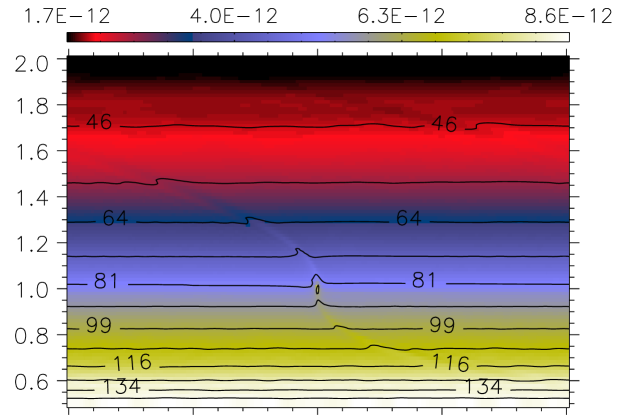
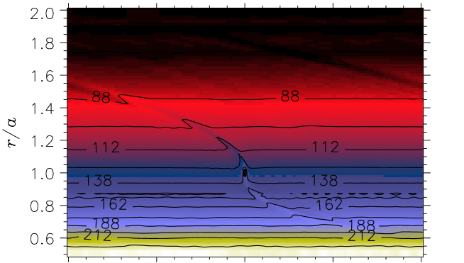
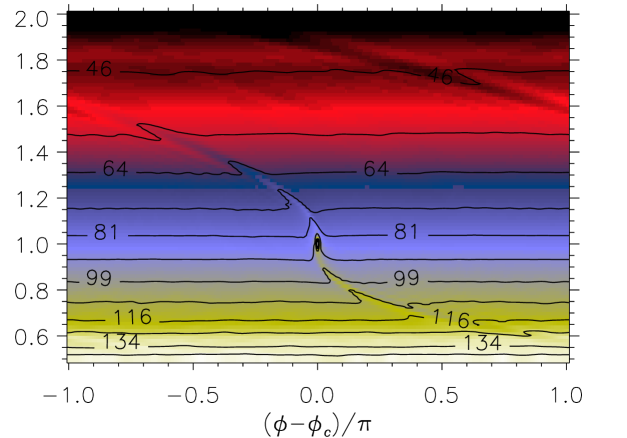
Figure 4.— Disk density (in units of $\mathrm{g\,cm}^{-3}$, color scale) and temperature (in units of $\mathrm{K}$, contours) in the disk’s equatorial plane. The planetary core has azimuthal angle $\phi_{c}$ and semimajor axis $a$. From top to bottom, the core has a mass $\mbox{$M_{c}$}=5$, $10$, and $15\,\mbox{$M_{\mathrm{E}}$}$ and is located at $5\,\mbox{AU}$ on the left and at $10\,\mbox{AU}$ on the right.

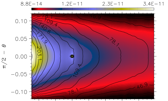
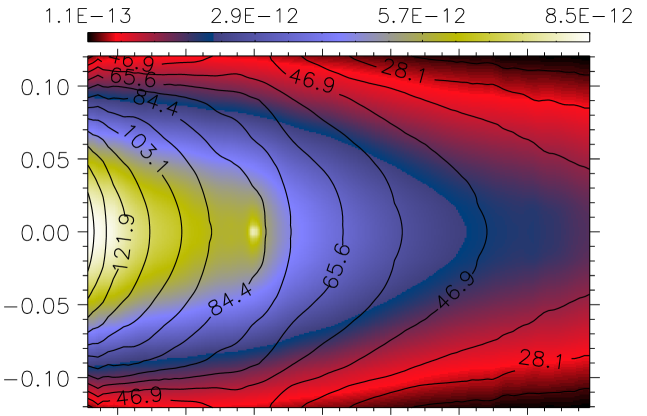
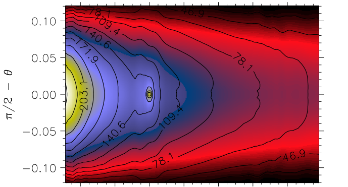
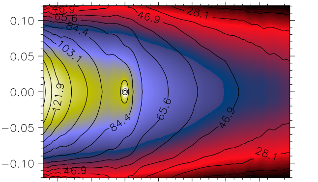
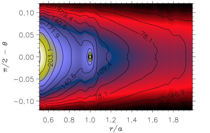
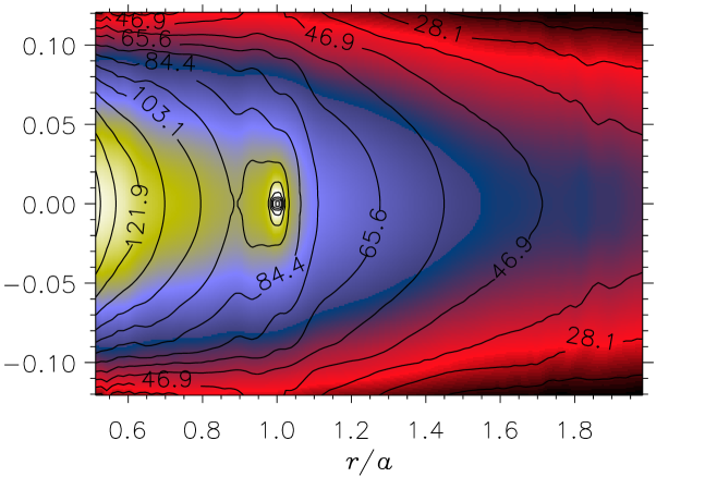
Figure 5.— As in Figure 4, but for the density and temperature in $r$–$\theta$ plane passing through the azimuthal position of the planetary core (at coordinates $r=a$ and $\theta=\pi/2$ in these maps). Embedded cores have masses $\mbox{$M_{c}$}=5$, $10$, and $15\,\mbox{$M_{\mathrm{E}}$}$ (from top to bottom), and orbital radii of $5\,\mbox{AU}$ (left) and $10\,\mbox{AU}$ (right).

The quasi-equilibrium density and temperature distributions, averaged in the azimuthal direction around the star in the disk mid-plane, is plotted in Figure 3. The solid lines refer to models with $a=5\,\mbox{AU}$ and the dashed lines to models with $a=10\,\mbox{AU}$. The mean radial slope of the density is such that $\langle\rho\rangle$ is roughly proportional to $r^{-3/2}$ around $5\,\mbox{AU}$, with a somewhat shallower slope around $10\,\mbox{AU}$. For the mid-plane temperature, the mean slope is roughly such that $\langle T\rangle\propto 1/r$. This slope is consistent with an approximate balance between viscous heating and vertical radiative cooling (e.g., D’Angelo et al., 2003a), considering that $\kappa_{\mathrm{R}}$ is either roughly proportional to $T^{0.1}$ or about constant at temperatures $40<T<250\,\mbox{$\mathrm{K}$}$ (Figure 14, lower-left panel). A summary of the azimuthally averaged disk’s properties, at the core’s orbital radius, is given in Table 1. Note that the results presented in Figure 3, and in the rest of this section, are plotted for the first grid level but calculated on the entire nested-grid structure (see Section 3.2).

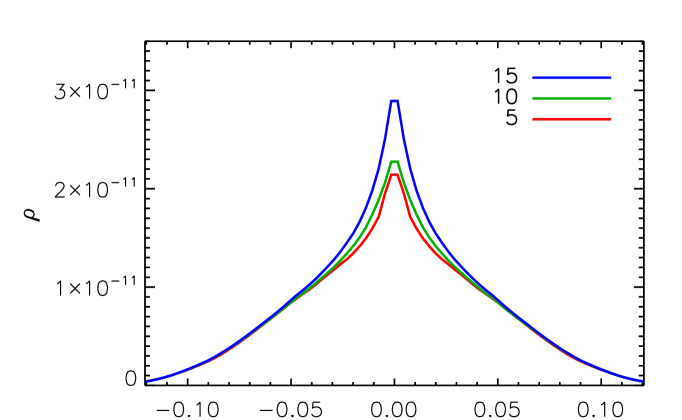
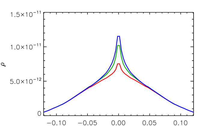
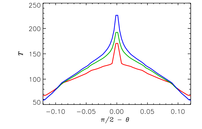
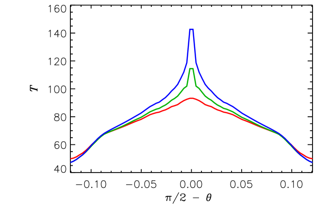
Figure 6.— Density in units of $\mathrm{g\,cm}^{-3}$ (top) and temperature in units of $\mathrm{K}$ (bottom), along the disk’s vertical (co-latitude) direction ($\theta=\pi/2$ indicates the mid-plane of the disk), at the radial and azimuthal position of the planetary core. The semimajor axis is $a=5\,\mbox{AU}$ in the left panels and $10\,\mbox{AU}$ in the right panels. The curves refer to cores of different mass, as listed in the top-left panel in units of $M_{\mathrm{E}}$.

The distributions of density and temperature in the disk’s equatorial plane are illustrated in Figure 4, where the images refer to the density and contour levels to the temperature (see the figure caption for further details). Similarly, Figure 5 shows the vertical stratification of density and temperature, at the azimuthal position of the planet. The effects of the core’s perturbation on the temperature in the equatorial plane are mostly confined to regions where compression occurs due to the propagation of spiral density waves. More local effects can be seen in Figure 5, where the isothermal (contour) lines indicate a temperature increase in the region around the radial position of the planet, an effect that becomes larger as the core mass increases. Density and temperature profiles in the vertical (i.e., $\theta$) direction, at the radial and azimuthal position of the core, are plotted in Figure 6. The figure shows the extent to which both density and temperature in the disk are enhanced, approaching the disk mid-plane ($\theta=\pi/2$), by gas compression due to the gravity of the planet. Effectively, these curves represent quantities averaged over the minimum spacing of the basic grid (see Section 3.2). In reality, as discussed in the next sections, density and temperature can be larger by orders of magnitudes in close proximity of the planet, but at distances from the core not resolved in these plots.

An estimate of disk aspect ratio can be obtained from the mid-plane temperature as $h\sim c_{\mathrm{gas}}/u_{\mathrm{K}}$, where $u_{\mathrm{K}}$ is the Keplerian velocity of the gas, so that $h\sim\sqrt{\Gamma_{1}k_{\mathrm{B}}Tr/(\mu m_{\mathrm{H}}G\mbox{$M_{\star}$})}$. The resulting aspect ratio is $\approx 0.06$ and $\approx 0.07$, respectively, for the disk models with $a=5$ and $10\,\mbox{AU}$. Since these values are computed using thermodynamical quantities at the mid-plane, they are likely to overestimate the value of $h$. Alternatively, the vertical density distribution can be approximated as hydrostatic, i.e., as a gaussian at any given radius. In a spherical geometry, said approximation corresponds to the profile along the $\theta$-direction $\exp{[(\sin\theta-1)/h^{2}]}$ (Masset et al., 2006). This procedure results in typical values of $h$, averaged over one scale height from the equatorial plane, of $\approx 0.055$ and $\approx 0.06$, respectively.

The azimuthally averaged density is not much affected by disk-planet tidal interactions, for any of the core masses considered, at both $5$ and $10\,\mbox{AU}$ (see left panel of Figure 3). Tidal perturbations are confined to the excitation of spiral density waves (see Figure 4). The absence of gap formation is in accord with simple arguments based on the balance of viscous and tidal torques exerted on the disk. In fact, when $\mbox{$R_{\mathrm{H}}$}/a<h$, the condition for significant tidal interactions (leading to gap formation) is approximately $(\mbox{$M_{c}$}/\mbox{$M_{\star}$})^{2}\gtrsim 3\pi\alpha h^{5}$ (e.g., D’Angelo & Lubow, 2010), assuming that the envelope mass $M_{e}$ is negligible. The equivalent $\alpha$-viscosity (Shakura & Syunyaev, 1973) in these disks at the planet’s orbital radius is $\alpha=\nu/(h^{2}a^{2}\Omega)\sim 0.001$, hence the condition above requires a core (plus envelope) mass $\gtrsim 30\,\mbox{$M_{\mathrm{E}}$}$ for significant tidal perturbation of the disk’s density.

5. Envelopes of Planetary Cores

There are two length scales that are relevant to the formation of a gaseous envelope around a solid core, both dictated by energy arguments. The first is determined by thermodynamics and the second by gravity.

The mean thermal velocity of the gas is $u_{\mathrm{th}}=\sqrt{(8/\pi)k_{\mathrm{B}}T/(\mu m_{\mathrm{H}})}$ (e.g., Mihalas & Weibel Mihalas, 1999). Disk gas moving within a maximum distance, $R_{\mathrm{B}}$, of a planetary core may become bound to the core if $u_{\mathrm{th}}$ is smaller than the escape velocity from the core at that distance, $u_{\mathrm{esc}}=\sqrt{2G\mbox{$M_{c}$}/\mbox{$R_{\mathrm{B}}$}}$ (e.g., Bodenheimer & Pollack, 1986), where

$$\mbox{$R_{\mathrm{B}}$}=\left(\frac{\pi}{4}\right)\frac{G\mbox{$M_{c}$}\mu m_{\mathrm{H}}}{k_{\mathrm{B}}T}$$ (37)

is the Bondi radius and is defined through the condition $u_{\mathrm{th}}=u_{\mathrm{esc}}$. The disk region where the gravity of the core dominates that of the star is set by the (circular) restricted three-body problem dynamics and is a fraction of the Hill radius, $\mbox{$R_{\mathrm{H}}$}=a\left[\mbox{$M_{c}$}/(3\mbox{$M_{\star}$})\right]^{1/3}$. In fact, the radius of the sphere having the same volume as the Roche lobe is $\approx 2\mbox{$R_{\mathrm{H}}$}/3$ (Paczyński, 1971; Kopal, 1978) and the radius of a sphere entirely contained in the Roche lobe is $\lesssim 3\mbox{$R_{\mathrm{H}}$}/5$, as can be calculated from the equations describing the equipotential surfaces of the three-body problem (e.g., Murray & Dermott, 2000).

Therefore, a gaseous envelope may form around a core within the smaller of $R_{\mathrm{B}}$ and $3\mbox{$R_{\mathrm{H}}$}/5$. These two characteristic lengths become equal for a core mass

$$\mbox{$M_{c}$}\approx\left[\frac{9}{2\mbox{$M_{\star}$}}\left(\frac{a}{\pi}\frac{k_{\mathrm{B}}T}{G\mu m_{\mathrm{H}}}\right)^{3}\right]^{1/2},$$ (38)

or $\mbox{$M_{c}$}/\mbox{$M_{\mathrm{E}}$}\approx 3.6\mu^{-3/2}(T/100\,\mbox{$\mathrm{K}$})^{3/2}(a/1\,\mbox{AU})^{3/2}$ for a solar-mass star (in the equation above, $(5/4)^{3}$ is approximated to $2$). In our disk models, at $5\,\mbox{AU}$, the ratio of the two lengths, $(5/3)\mbox{$R_{\mathrm{B}}$}/\mbox{$R_{\mathrm{H}}$}$, varies from $\approx 0.5$ ($\mbox{$M_{c}$}=5\,\mbox{$M_{\mathrm{E}}$}$) to $\approx 1$ ($\mbox{$M_{c}$}=15\,\mbox{$M_{\mathrm{E}}$}$). At $10\,\mbox{AU}$, the Bondi radius is larger by a factor of about $3/2$ (due to the lower disk temperature, see Figure 3), but the Hill radius is twice as large. Therefore, the ratio of the characteristic lengths is reduced by a factor of $4/3$. In all cases considered here, the envelope radius should be generally set by thermal arguments ($\mbox{$R_{\mathrm{B}}$}\lesssim 3\mbox{$R_{\mathrm{H}}$}/5$). The envelope is therefore expected to be confined within the Bondi sphere and the Bondi radius is expected to be a hard limit for the envelope radius. Note that additional energy sources, such as kinetic energy of the background flow, may facilitate gas escape from the core at even shorter distances.

It should be stressed that while $R_{\mathrm{H}}$ has a non-ambiguous definition (if the mass contributed by a planet’s envelope is small compared to $M_{c}$, as in these calculations), there is an ambiguity in the definition of $R_{\mathrm{B}}$, since it relies on an average temperature of the background flow. In the estimates given above, this temperature is taken as the azimuthal average (around the star) at the planet’s orbital radius. In reality, the temperature should be some local mean calculated outside, but in the vicinity (i.e., on the length scale), of the envelope radius. As a local mean around the planet, such temperature is expected to be somewhat larger than the disk azimuthal average and also to depend on the core mass. Therefore, the Bondi radius may be somewhat smaller than the estimates presented above and Equation (37) should represent an upper bound. In the following, to make the definition less ambiguous and more workable for our purposes, we shall refer to this upper bound as the nominal length of the Bondi radius.

5.1. 1D Calculations of Envelopes

We perform 1D calculations of the accumulation of gaseous envelopes around planetary cores using the planet evolution code of Pollack et al. (1996); Hubickyj et al. (2005); Lissauer et al. (2009), and references therein. We also apply the procedures and approximations detailed in those papers. The purpose of the 1D calculations is to produce reference models for the envelope stratification (e.g., of temperature and density) around cores of $5$, $10$, and $15\,\mbox{$M_{\mathrm{E}}$}$, at both $5$ and $10\,\mbox{AU}$. Additionally, they provide the core accretion rate $\dot{M}_{c}$ that is needed for the energy source term in Equation (10), which represents the gravitational energy released at the base of the envelope by incoming solid material.

In these models, a $0.1\,\mbox{$M_{\mathrm{E}}$}$ core accretes solids (planetesimals of $100\,\mathrm{km}$ in radius) and gas. The accretion rate of planetesimals is proportional to the local surface density of solids. We use values of $10$ and $13\,\mathrm{g\,cm^{-2}}$ for cores forming at $5\,\mbox{AU}$, and $6\,\mathrm{g\,cm^{-2}}$ for cores forming at $10\,\mbox{AU}$. Given the gas-to-dust mass ratio of $\approx 70$ assumed here (see Appendix A for details), such values are consistent with the expected gas-augmented initial surface density ($\approx 2000\,\mathrm{g\,cm^{-2}}$ or less at $1\,\mbox{AU}$) in the disks described in Section 4.

In standard core accretion calculations, the cross-over mass, $\mbox{$M_{c}$}=\mbox{$M_{e}$}$, is about equal to $\sqrt{2}$ times the isolation mass (Pollack et al., 1996). Since the 3D radiation hydrodynamics calculations performed for this study neglect the effects of gas self-gravity, we should restrict the discussion to earlier phases of the planet evolution when the envelope is still much less massive than the core. At $5\,\mbox{AU}$, the cross-over mass is about $15\,\mbox{$M_{\mathrm{E}}$}$ when the surface density of solids is $10\,\mathrm{g\,cm^{-2}}$. For a solids’ surface density of $13\,\mathrm{g\,cm^{-2}}$, the cross-over mass is instead $\approx 22\,\mbox{$M_{\mathrm{E}}$}$, and $\mbox{$M_{e}$}\ll\mbox{$M_{c}$}$ when $\mbox{$M_{c}$}=15\,\mbox{$M_{\mathrm{E}}$}$ (see Section 5.2). At $10\,\mbox{AU}$, the cross-over mass ($\propto a^{3}$) is larger than $50\,\mbox{$M_{\mathrm{E}}$}$ in the 1D models considered here.

The accretion rate of gas is dictated by the contraction rate of the envelope. At these early stages of formation, it mainly depends on the ability of the outer envelope to cool by radiating away the gravitational energy produced by contraction and by the accretion of planetesimals. Since dust grains represent the main source of opacity in the outer envelope, their optical properties, abundance, and depth distribution are critical to the determination of the gas accretion rate (Movshovitz et al., 2010). Our 1D models use interstellar dust opacities (Pollack et al., 1985) reduced by a factor $50$, to mimic the reduction caused by grain growth and settling in the envelope (Podolak, 2003). As explained in the next section (see also Appendix A), the 3D calculations use different dust opacities, applying a size distribution of grains whose presence in T Tauri disks is suggested by observations. These opacities also fall well below interstellar values in the relevant temperature range.

The exterior boundary of the envelope is defined as in Lissauer et al. (2009), so that the inverse of the envelope radius is equal to $1/\mbox{$R_{\mathrm{B}}$}+4/\mbox{$R_{\mathrm{H}}$}$. Note that for $\mbox{$R_{\mathrm{B}}$}\approx\mbox{$R_{\mathrm{H}}$}$, the envelope radius becomes $\approx\mbox{$R_{\mathrm{B}}$}/5$. At the exterior boundary, densities and temperatures are matched to the disk values, azimuthally averaged around the star, obtained from the 3D calculations and given in Table 1. Therefore, we set $\rho=1.3\times 10^{-11}\,\mathrm{g\,cm^{-3}}$ and $T=124\,\mbox{$\mathrm{K}$}$ at $5\,\mbox{AU}$, and $\rho=5\times 10^{-12}\,\mathrm{g\,cm^{-3}}$ and $T=80\,\mbox{$\mathrm{K}$}$ at $10\,\mbox{AU}$ (see also Figure 3).

5.2. Comparisons between 1D and 3D Envelopes

Table 2Envelope Masses and Accretion Rates in 1D and 3D Models

		$5\,\mbox{$M_{\mathrm{E}}$}$				$10\,\mbox{$M_{\mathrm{E}}$}$				$15\,\mbox{$M_{\mathrm{E}}$}$
$a$		$\dot{M}_{c}$	$\dot{M}_{e}$	$M_{e}$		$\dot{M}_{c}$	$\dot{M}_{e}$	$M_{e}$		$\dot{M}_{c}$	$\dot{M}_{e}$	$M_{e}$
$5$		$8.8\times 10^{-5}$	$9.5\times 10^{-8}$	$1.8\times 10^{-3}$		$5.9\times 10^{-5}$	$1.4\times 10^{-6}$	$3.2\times 10^{-2}$		$1.2\times 10^{-4}$	$4.0\times 10^{-6}$	$8.1\times 10^{-2}$
$10$		$5.6\times 10^{-5}$	$8.4\times 10^{-8}$	$2.8\times 10^{-3}$		$1.2\times 10^{-4}$	$6.9\times 10^{-7}$	$1.9\times 10^{-2}$		$1.8\times 10^{-4}$	$2.0\times 10^{-6}$	$6.5\times 10^{-2}$
		$\dot{M}_{c}$[3D]	$\dot{M}_{e}$[3D]	$M_{e}$[3D]		$\dot{M}_{c}$[3D]	$\dot{M}_{e}$[3D]	$M_{e}$[3D]		$\dot{M}_{c}$[3D]	$\dot{M}_{e}$[3D]	$M_{e}$[3D]
$5$		$8.8\times 10^{-5}$	$1.5\times 10^{-7}$	$1.3\times 10^{-3}$		$5.9\times 10^{-5}$	$8.7\times 10^{-7}$	$1.8\times 10^{-2}$		$1.2\times 10^{-4}$	$2.1\times 10^{-6}$	$3.5\times 10^{-2}$
$10$		$5.6\times 10^{-5}$	$9.2\times 10^{-8}$	$1.6\times 10^{-3}$		$1.2\times 10^{-4}$	$5.1\times 10^{-7}$	$8.7\times 10^{-3}$		$1.8\times 10^{-4}$	$1.4\times 10^{-6}$	$3.3\times 10^{-2}$

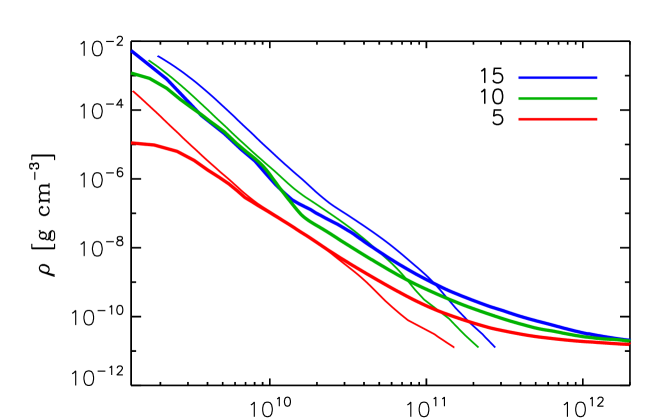
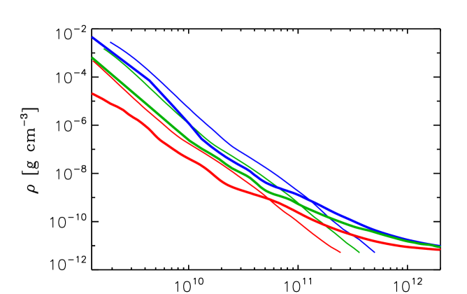
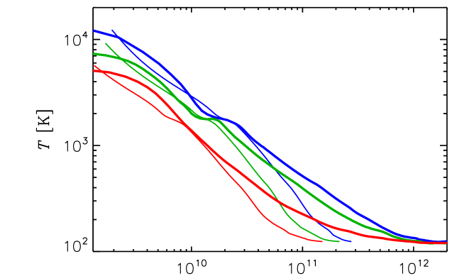
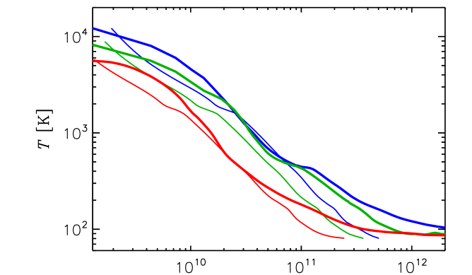
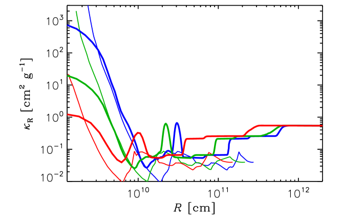
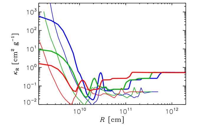
Figure 7.— Averaged density (top), temperature (center), and Rosseland mean opacity (bottom), versus distance from the core center, of 3D envelopes around planetary cores of different masses, as indicated in the legend of the top-left panel in units of $M_{\mathrm{E}}$. The cores are located at $5$ (left) and $10\,\mbox{AU}$ (right). The thinner lines, which start at the core radius $R_{c}$ (between $\approx 1.3\times 10^{9}$ and $\approx 1.9\times 10^{9}\,\mathrm{cm}$), represent the same quantities obtained from the 1D models discussed in Section 5.1.

Some bulk quantities of the 1D and 3D envelope models are reported in Table 2. As explained above, $\dot{M}_{c}$ is calculated in the 1D models and applied to the 3D calculations (hence the same entries in the table), in order to modify the energy budget of the gas on a length scale $\approx R_{c}$ around the core. For consistency, the envelope masses $M_{e}$[3D] are computed using the same envelope radii as in the 1D models. The gas accretion rate of the 3D envelopes, $\dot{M}_{e}$[3D], is evaluated from the change of the envelope mass over a time of roughly $50$ orbits of the core.

The envelope masses reported in Table 2 also allow us to evaluate possible effects caused by the envelope gravity, which are unaccounted for in the 3D calculations. In fact, the ratio of the radial component (i.e., toward the core center) of the gravitational force due to the gas and that due to the core is at most $\mbox{$M_{e}$}/\mbox{$M_{c}$}$. According to 1D models, this ratio ranges from $10^{-4}$ to $10^{-3}$, and similar ratios result from the 3D models. Hence, only a relatively small contribution is expected to arise from the envelope gravity at these stages of evolution.

There are several physical differences between the 1D and the 3D calculations. In particular, the 1D models are computed as a sequence of hydrostatic envelope structures whereas the 3D models are intrinsically hydrodynamical, with a complex velocity field. Diffusion and convection of energy are mutually exclusive in the 1D calculations (and the adiabatic temperature gradient is applied to the convective layers) whereas they always occur together in the 3D calculations, through an advection-diffusion equation (see Section 2.2), regardless of which transport mechanism is dominant. Conversion of mechanical energy into thermal energy, determined by viscosity through Equation (11), is taken into account in the 3D, but not in the 1D, calculations. The release of energy by planetesimals penetrating the envelope occurs gradually and is depth-dependent in the 1D models, whereas all the energy is released at the bottom of the envelope in the 3D models, effectively as if no ablation took place and planetesimals were intact upon hitting the core. The dust opacity of the outer layers of the envelope is different, typically lower in the 1D models.

Considering all these differences and the fact that some properties of 1D envelopes are related to their history, we should only seek for consistency between 1D and 3D calculations. In this sense, the bulk quantities reported in Table 2 do show a general agreement: both envelope masses and gas accretion rates, $\dot{M}_{e}$, differ by factors of $2$ or less. In particular, as gas accretion is a consequence of contraction, the numbers in the Table suggest that the contraction time scales of the 1D and 3D envelopes are comparable. The relative increase of $\dot{M}_{e}$, for increasing core mass, is also comparable. It is important to notice that gas accretion rates differ by factors of oder unity, between calculations with $a=5$ and $10\,\mbox{AU}$ (in both 1D and 3D), an indication that they are dictated by the internal envelope properties, as just mentioned, rather than imposed by the external disk thermodynamics (which is different at the two orbital locations, see Section 4).

Figure 7 shows a more detailed comparison, between the 1D and 3D calculations, of the density (top), temperature (center), and Rosseland mean opacity (bottom), versus distance from the core center, $R$, for values of the ratio $\mbox{$M_{c}$}/\mbox{$M_{\mathrm{E}}$}$ indicated in the legend of the top-left panel. Left panels refer to planets with a semimajor axis of $5\,\mbox{AU}$ and right panels refer to planets with $a=10\,\mbox{AU}$. The envelope properties of the 1D calculations (thin lines) are similar at the two orbital radii, except in the outer parts because of the different boundary conditions (see Section 5.1). The results from the 3D calculations (thick lines), computed as averages around the core at $\theta=\pi/2$ and plotted up to a distance $R>\mbox{$R_{\mathrm{H}}$}/2$, show a somewhat larger contrast between cases at $5$ and $10\,\mbox{AU}$. Overall, the 3D envelope models are less dense in the interiors, denser in the outer parts, and generally hotter than the 1D envelope models.

Differences should be expected at length scales of order $R_{c}$ from the core ($1.3\times 10^{9}\lesssim R_{c}\lesssim 1.9\times 10^{9}\,\mathrm{cm}$), as the 3D models have a linear resolution between about $R_{c}$ and $2\,R_{c}$, while the resolution of the 1D models is better by two (or more) orders of magnitude! The gravitational potential is also different at $R_{c}$, since the 3D calculations use a softened potential (see Appendix D), producing a shallower gravity field. Despite these limitations, thermodynamical quantities at the base of the envelope are comparable in most cases. In the 1D models, the density at $R_{c}$ ranges from $\approx 4\times 10^{-4}$ to $\approx 4\times 10^{-3}\,\mathrm{g\,cm^{-3}}$, the temperature varies from $\approx 5700$ to $\approx 12000\,\mbox{$\mathrm{K}$}$, and the pressure is between $\approx 10^{8}$ and $\approx 3\times 10^{9}\,\mathrm{dyne\,cm^{-2}}$. In the 3D models, the density at the core ranges from $\approx 10^{-5}$ to $\approx 10^{-3}\,\mathrm{g\,cm^{-3}}$, the temperature varies from $\approx 5000$ to $\approx 11000\,\mbox{$\mathrm{K}$}$, and the gas pressure is between $\approx 10^{6}$ and $\approx 4\times 10^{9}\,\mathrm{dyne\,cm^{-2}}$. The largest discrepancies at the base of the envelope occur for the density (and hence pressure) around the $5\,\mbox{$M_{\mathrm{E}}$}$ cores, as visible in the top panels of Figure 7, although the case at $5\,\mbox{AU}$ is also the one that displays the best agreement with the 1D calculation beyond a few core radii.

Differences in density, temperature, and pressure are also expected at the outer radius of the 1D envelopes, as values there are affected by the boundary conditions (see discussion in Section 5.1). At that distance from the core, between $10^{11}$ and $5\times 10^{11}\,\mathrm{cm}$, the density of the 3D envelopes is larger by factors between $7$ and $12$, the temperature is higher by factors between $1.5$ and $2$, and the gas pressure is greater by factors between $10$ and $25$. These factors also represent the largest relative differences, between the 1D and 3D calculations, in the density and temperature distributions throughout most of the envelope ($R\gtrsim 3\,R_{c}$).

The Rosseland mean opacity in the envelope, of both gas and dust, is illustrated in the bottom panels of Figure 7 (see the lower-left panel of Figure 14 for a plot of $\kappa_{\mathrm{R}}$ as a function of temperature). Distinct transitions can be seen, corresponding to the sublimation/formation of the various grain species included in the opacity calculation (see Appendix A). The most prominent transitions are those associated with the vaporization of water ice grains at $T\approx 160\,\mbox{$\mathrm{K}$}$ and of refractory organics grains at $T\approx 420\,\mbox{$\mathrm{K}$}$ (the average temperatures at the outer radius of the 3D envelopes, defined in the next section, are $\lesssim 160\,\mbox{$\mathrm{K}$}$). Minor transitions can also be identified, such as the one corresponding to the sublimation of troilite (FeS) at $T\approx 680\,\mbox{$\mathrm{K}$}$. The reduction of opacity due to the vaporization deeper in the envelope of more refractory species, such as silicates at $T\gtrsim 1400\,\mbox{$\mathrm{K}$}$ when $\rho\gtrsim 10^{-8}\,\mathrm{g\,cm^{-3}}$, is compensated for by the increase of molecular opacity, which peaks around $2000\,\mbox{$\mathrm{K}$}$ (see Ferguson et al., 2005). At temperatures below the sublimation temperature of refractory organics, the opacity of the 3D envelopes is larger than that of the 1D envelopes, on average by factors of $5$–$7$. Above such temperature, and up to $\sim 1500\,\mbox{$\mathrm{K}$}$, the opacities differ by a factor $2$, or less. As can be seen in the lower-left panel of Figure 14, between $\sim 100$ and $\sim 1000\,\mbox{$\mathrm{K}$}$ the opacity of the 3D models is a factor $\sim 10$ lower than the interstellar dust opacity (due to the presence of larger grains). The grain opacity of 1D models is interstellar, but reduced by a factor $50$. In the envelope interiors, differences in (gas) opacity are likely less relevant as energy transport is expected to occur mostly via convection.

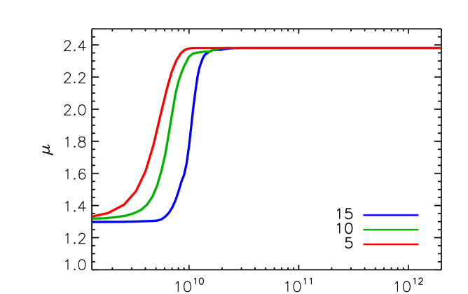
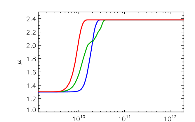
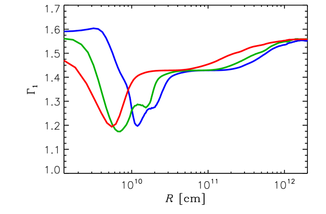
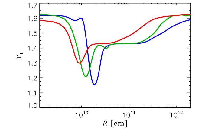
Figure 8.— Average values of the mean molecular weight, $\mu$, in Equation (19) (top) and of the first adiabatic exponent,$\Gamma_{1}$, in Equation (26) (bottom), versus distance from the core center, in 3D envelopes around cores of various masses, as indicated in the top-left panel in units of $M_{\mathrm{E}}$. Left and right panels refer to the core’s orbital radius of $5$ and $10\,\mbox{AU}$, respectively.

The mean molecular weight (Equation (19)) and the first adiabatic exponent (Equation (26)) of the gas in the envelope are plotted in Figure 8, for all core masses. The left and right panels refer, respectively, to cases with semimajor axis of $5$ and $10\,\mbox{AU}$. Significant dissociation of $\mathrm{H}_{2}$ begins at $T\sim 1500\,\mbox{$\mathrm{K}$}$ ($\rho\sim 10^{-8}\,\mathrm{g\,cm^{-3}}$) and is nearly complete (when $\mu\simeq 1.3$) at $T\gtrsim 4000\,\mbox{$\mathrm{K}$}$, depending on the local gas density (see Figure 2). The dissociation begins farther away from the core, at a distance about $25$% greater, in the model with $\mbox{$M_{c}$}=10\,\mbox{$M_{\mathrm{E}}$}$ at $10\,\mbox{AU}$ than in the $15\,\mbox{$M_{\mathrm{E}}$}$ case at the same orbital distance (see top-right panel) because of the similar temperatures but lower densities. Otherwise, the volume of atomic hydrogen increases as the core mass becomes larger. No significant ionization is observed deep in the envelope. The first adiabatic exponent, in the bottom panels, dips to a minimum during the dissociation of $\mathrm{H}_{2}$. The curves also show, to the right of the minimum, the reduction of $\Gamma_{1}$ caused by the excitation of vibrational and rotational states of $\mathrm{H}_{2}$ (see Figure 1).

5.3. Size, Shape, and Rotation of 3D Envelopes

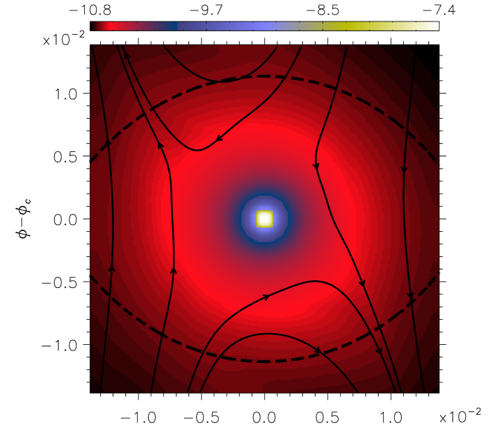
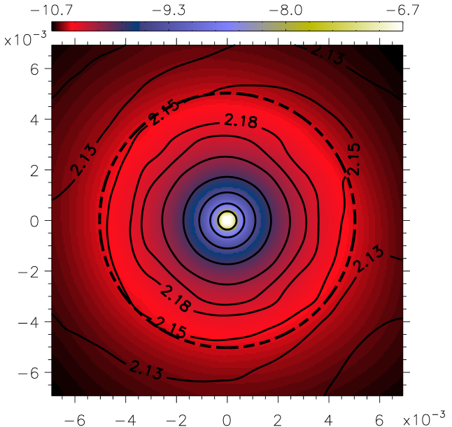
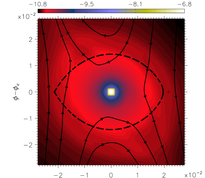
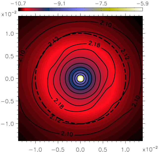
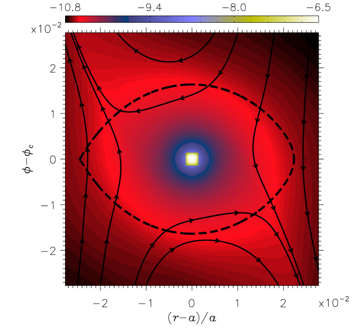
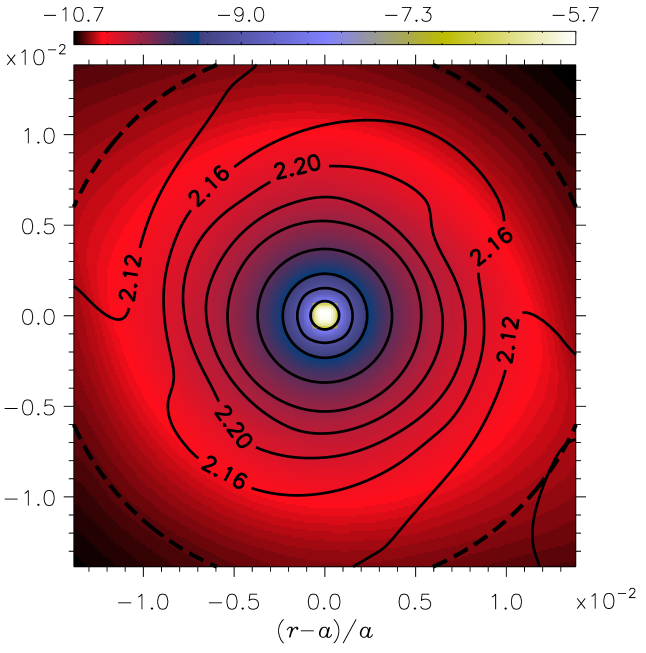
Figure 9.— Density around the envelope region (on a logarithmic scale in units of $\mathrm{g\,cm}^{-3}$) in the disk mid-plane, for planetary cores located at $5\,\mbox{AU}$. From top to bottom, the core mass is $5$, $10$, and $15\,\mbox{$M_{\mathrm{E}}$}$. The density is saturated around the core position to improve the scale contrast. The left panels also show the flow streamlines at the mid-plane, along with the intersection with the Roche lobe (dashed line). The right panels show the temperature contours (on a logarithmic scale in units of $\mathrm{K}$). The dashed circle represents the intersection with the Bondi sphere (see Section 5).

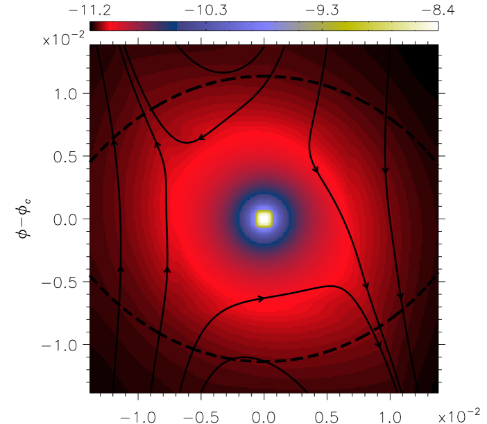
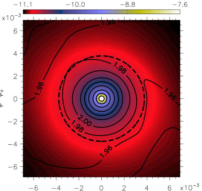
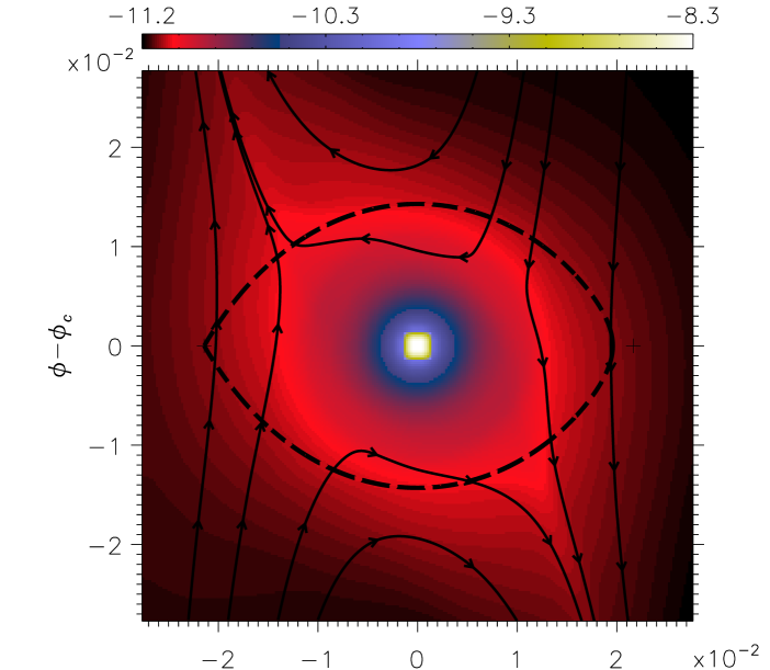
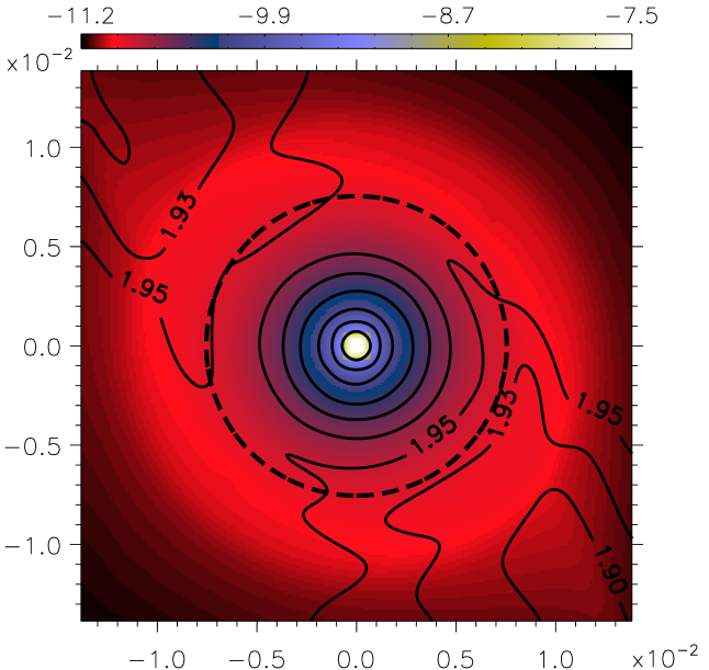
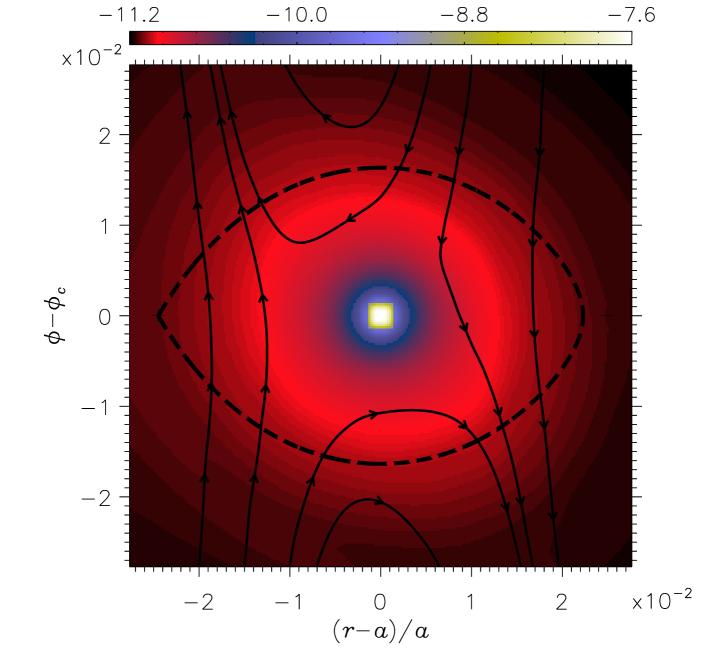
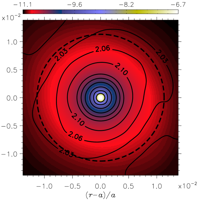
Figure 10.— Same quantities as in Figure 9, but around cores located at $10\,\mbox{AU}$.

We wish to identify a volume around the core that can be defined as its “envelope”. Gas inside this volume does not participate in the disk circulation any longer. If the gas behaved as a collision-less system only subjected to gravity, the Roche lobe would define such a volume. For simplicity, we assume that the envelope is a sphere.

Figures 9 and 10 show density maps, flow streamlines at the mid-plane (left panels), and temperature contours (right panels) in regions around cores located at $5$ and $10\,\mbox{AU}$, respectively (see the caption of Figure 9 for further details). Also plotted in the panels are the intersection of the core’s Roche lobe (left) and Bondi sphere (right) with the disk mid-plane ($\theta=\pi/2$). The streamlines clearly indicate that the volume of each envelope must be significantly smaller than that of the corresponding Roche lobe. In fact, horse-shoe or circulating orbits reach as close to the core as $0.4\,\mbox{$R_{\mathrm{H}}$}$. Symmetry properties of the gas may also help to identify the envelope region. Contours of equal temperature suggest that each envelope is confined within the corresponding Bondi sphere (Equation (37)), as also argued in Section 5. Based on the shape of these contours illustrated in the right panels of Figures 9 and 10, the envelopes would appear to extend over radii between $\approx 0.4$ and $\approx 0.6\,\mbox{$R_{\mathrm{B}}$}$. These contours also suggest that, in units of $R_{\mathrm{B}}$, the envelope radius tends to be smaller for larger cores.

There is no obvious reason, though, that justifies the spherical symmetry assumption of thermodynamical quantities for a non-isolated planet, particularly in the outer envelope layers, which are likely affected by interactions with the flow circulation exterior to the envelope. Layers whose density and pressure are comparable to those of the external flow are the most affected, and their dynamics must bear some similarities to that of the unbound gas in contact with the envelope. In other words, the properties of these envelope layers must be affected by the accretion flow, which need not be (and is not!) spherically symmetric around the core (see Section 5.4). Consequently, symmetry arguments may not be appropriate to define the outer envelope regions, and tracking of the actual motion of the gas is then necessary to determine the envelope volume.

Table 3Envelope Properties from the 3D Models

$a$	$M_{c}$	$M_{e}$	$R_{e}$	$I_{11}$	$I_{22}$	$I_{33}$	$I_{12}$	$L_{3}$	$\omega_{3}$	$b_{3}/b_{1}$	$b_{3}/b_{2}$
[AU]	[$M_{\mathrm{E}}$]	[$M_{\mathrm{E}}$]	[$a$]	[$\mbox{$M_{e}$}R^{2}_{e}$]	[$\mbox{$M_{e}$}R^{2}_{e}$]	[$\mbox{$M_{e}$}R^{2}_{e}$]	[$\mbox{$M_{e}$}R^{2}_{e}$]	[$\mbox{$M_{e}$}R^{2}_{e}\Omega$]	[$\Omega$]
$5$	$\phantom{1}5$	$2.5\times 10^{-3}$	$0.0046$	$0.207$	$0.208$	$0.209$	$\phantom{-}9.4\times 10^{-5}$	$1.07\times 10^{-2}$	$0.05$	$0.988$	$0.991$
$5$	$10$	$2.2\times 10^{-2}$	$0.0065$	$0.096$	$0.096$	$0.101$	$-3.3\times 10^{-5}$	$1.37\times 10^{-1}$	$1.36$	$0.949$	$0.951$
$5$	$15$	$4.9\times 10^{-2}$	$0.0096$	$0.131$	$0.132$	$0.138$	$-7.0\times 10^{-5}$	$4.41\times 10^{-1}$	$3.19$	$0.944$	$0.953$
$10$	$\phantom{1}5$	$2.2\times 10^{-3}$	$0.0026$	$0.220$	$0.220$	$0.221$	$-1.7\times 10^{-5}$	$1.62\times 10^{-2}$	$0.07$	$0.996$	$0.997$
$10$	$10$	$1.0\times 10^{-2}$	$0.0036$	$0.192$	$0.193$	$0.194$	$-1.0\times 10^{-4}$	$2.08\times 10^{-1}$	$1.07$	$0.990$	$0.992$
$10$	$15$	$3.5\times 10^{-2}$	$0.0045$	$0.106$	$0.106$	$0.107$	$-2.5\times 10^{-5}$	$1.47\times 10^{-1}$	$1.38$	$0.988$	$0.989$

We follow the approach of Lissauer et al. (2009) and use passive tracers to characterize the motion of gas around a core and determine the volume where gas is bound to the core. The tracer particles are advected by the flow, and thus follow the trajectory of gas parcels. The position of the tracers is advanced in time according to the method described in Appendix D of D’Angelo & Lubow (2008). The trajectories are second-order accurate in both space and time, and use velocity fields at the highest resolution available. The particles are deployed on concentric spherical surfaces centered at the core center. The spheres have radii ranging from $\approx R_{c}$ to $3\mbox{$R_{\mathrm{H}}$}/5$, the largest possible radius of an envelope when $R_{\mathrm{B}}$ exceeds this distance (see discussion in Section 5). In total, $60000$ tracers are deployed on the northern hemisphere of $50$ spherical shells. Mirror symmetry conditions are applied to positions and velocities of tracers that cross the equatorial plane toward the southern hemisphere. Denoting with $s(t)$ the distance from the center of the core ($R=0$) along the trajectory of a particle, the envelope radius is taken as the radius $R_{e}$ of the largest spherical surface for which $s_{i}(t)\leq 3\mbox{$R_{\mathrm{H}}$}/5$, for all tracers $i$ initially deployed on that surface. For sensitivity purposes, one calculation also uses $360000$ tracers distributed on $100$ hemispheres, but no significant difference is observed.

Particles that travel beyond $3\mbox{$R_{\mathrm{H}}$}/5$ are either on horse-shoe or circulating orbits (see left panels of Figures 9 and 10), and rapidly leave the region. At the end of the trajectory integrations, tracers are either located inside the envelope ($R\leq R_{e}$) or in the disk, and no particle is left between $R_{e}$ and $3\mbox{$R_{\mathrm{H}}$}/5$. A fraction of the tracers deployed outside of the envelope do move inside the envelope. These tracers define the accretion flow that will be discussed in the next section.

The estimates of the envelope radius are listed in the fourth column of Table 3, preceded by the envelope mass, $M_{e}$, contained within this radius. (Notice that the masses $M_{e}$[3D] in Table 2 are those inside the envelope radii of the 1D calculations.) The radius $R_{e}$ increases with core mass and, for a given $M_{c}$, varies by $\lesssim 10$% with respect to the orbital distances. The ratio $R_{e}/\mbox{$R_{\mathrm{B}}$}$ decreases with increasing core mass. The cores located at $5\,\mbox{AU}$ have radii between $0.64$ and $0.92\,\mbox{$R_{\mathrm{B}}$}$, and between $0.40$ and $0.69\,\mbox{$R_{\mathrm{B}}$}$ at $10\,\mbox{AU}$. In terms of Hill radius, the cores at $5\,\mbox{AU}$ have envelope radii smaller than $\approx\mbox{$R_{\mathrm{H}}$}/3$ and smaller than $\mbox{$R_{\mathrm{H}}$}/5$ at $10\,\mbox{AU}$. Overall, these results are consistent with the energy-based arguments of Section 5, according to which $R_{e}\lesssim\mbox{$R_{\mathrm{B}}$}$ if $\mbox{$R_{\mathrm{B}}$}<\mbox{$R_{\mathrm{H}}$}$. They are also in agreement with the analysis based on the streamlines, discussed above, according to which $R_{e}\lesssim 0.4\,\mbox{$R_{\mathrm{H}}$}$. Moreover, as argued above, spherical symmetry of, e.g., isothermal surfaces should not be expected in the outer envelope layers of non-isolated planets.

The densities at $R=R_{e}$ are between $3.5\times 10^{-11}$ and $\approx 5\times 10^{-11}\,\mathrm{g\,cm^{-3}}$ at $a=5\,\mbox{AU}$, and between $2\times 10^{-11}$ and $\approx 3\times 10^{-11}\,\mathrm{g\,cm^{-3}}$ at $a=10\,\mbox{AU}$, $3$ to $6$ times larger than the azimuthally averaged densities around the star. The temperatures range from $\approx 140$ to $\approx 160\,\mbox{$\mathrm{K}$}$ and from $\approx 100$ to $\approx 140\,\mbox{$\mathrm{K}$}$ at the smaller and larger orbital distance, respectively. The perturbed temperatures are $\lesssim 30$% ($a=5\,\mbox{AU}$) and $\lesssim 75$% ($a=10\,\mbox{AU}$) higher than the corresponding azimuthally averaged temperatures around the star (see Table 1).

Let us introduce a cartesian reference frame, whose origin is attached to the center of the core and in which $\{x_{i}\}$, with $i=1$, $2$, and $3$, indicate the coordinate axes. The axis $x_{1}$ is parallel to the core-star direction, pointing toward the star; axis $x_{2}$ is tangent to the orbit, pointing in the opposite direction of the orbital motion; axis $x_{3}$ is perpendicular to the orbit, so that $\boldsymbol{\hat{x}}_{1}\boldsymbol{\times}\boldsymbol{\hat{x}}_{2}=\boldsymbol{\hat{x}}_{3}$.

In order to determine some bulk properties, such as rotation and flattening, we shall assume that the envelope can be approximated as a rigid body and introduce the inertia tensor (Landau & Lifshitz, 1976)

$$I_{ij}=\int_{V_{e}}\left(\delta_{ij}\sum_{k}x^{2}_{k}-x_{i}x_{j}\right)\rho dV,$$ (39)

where $V_{e}=(4\pi/3)R^{3}_{e}$ is the volume comprising the envelope. The diagonal components $I_{ii}$ are the moments of inertia of the envelope about the corresponding axes, and the negative of the off-diagonal components are the products of inertia. Equation (39) implies that $I_{ij}=I_{ji}$, hence only six elements of the tensor matrix are independent. Furthermore, by construction the envelope is symmetric with respect to the $x_{1}$–$x_{2}$ plane (see Section 2.1), therefore $I_{13}=I_{23}=0$.

The angular momentum with respect to the origin is

$$\boldsymbol{L}=\int_{V_{e}}\boldsymbol{x}\boldsymbol{\times}\boldsymbol{\dot{x}}\rho dV,$$ (40)

whose components for a rigid body can be expressed as

$$L_{i}=\sum_{j}I_{ij}\omega_{j},$$ (41)

where $\omega_{i}$ indicates the rotation rate about the axis $x_{i}$. From Equation (40) and from the assumed symmetry relative to the $x_{1}$–$x_{2}$ plane, we have that $L_{1}=L_{2}=0$. Thus, from Equation (41), it follows that $\omega_{1}=\omega_{2}=0$, whereas the rotation rate about axis $x_{3}$ is $\omega_{3}=L_{3}/I_{33}$. Note that $\omega_{3}>0$ corresponds a counter-clockwise rotation, in the same direction as the orbital revolution.

Due to symmetry, axis $x_{3}$ is a principal axis of inertia while axes $x_{1}$ and $x_{2}$ are not, since the inertia tensor is not diagonal. In fact, as reported in Table 3, $I_{12}\neq 0$. However, the table shows than $|I_{12}|\ll I_{ii}$ in all cases and therefore axes $x_{1}$ and $x_{2}$ can be considered as principal axes to a very good approximation. Comparing $I_{33}$ of the envelopes at $a=5$ and $10\,\mbox{AU}$, a significant difference (a factor $2$) is found only for $15\,\mbox{$M_{\mathrm{E}}$}$ case. Otherwise, they agree to a level better than $20$%.

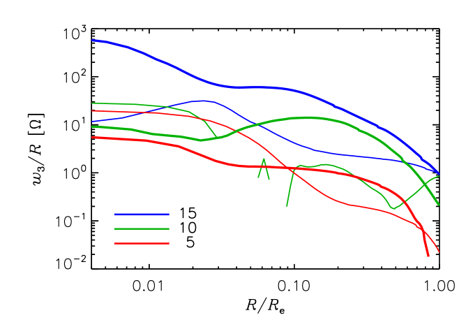
Figure 11.— Average angular velocity of the gas about the polar axis $x_{3}$, in the equatorial plane of the envelope ($\theta=\pi/2$). The quantity $w_{3}$ denotes the rotational velocity about the axis. Positive values indicate a counter-clockwise rotation. Gaps in the curves represent negative values of $w_{3}$. The thick (thin) lines refer to the core’s orbital radius $a=5\,\mbox{AU}$ ($10\,\mbox{AU}$). The core mass in units of $M_{\mathrm{E}}$ is indicated in the legend.

Table 3 also includes the values of $L_{3}$ and $\omega_{3}$, which imply that the envelopes are slow rotators, unless the rigid-body approximation is grossly inapplicable. We compute the average rotational velocity of the gas, $w_{3}$, about the axis $x_{3}$ in the equatorial plane. In Figure 11, we plot the angular velocity $w_{3}/R$ as a function of the distance from the axis. There is differential rotation at the equator, and the normalized derivative $d\ln{(w_{3}/R)}/d\ln{R}$ averages out to values between $\approx 0$ and $\approx-2$ for $0.1\lesssim R/R_{e}\lesssim 1$. Although the physical nature of $w_{3}/R$ and $\omega_{3}$ are quite different, it is plausible that $\omega_{3}$ samples the rotation of the outer envelope (carrying most of the angular momentum $L_{3}$) rather than that of the interior. If this is indeed the case, the slow rotation predicted by $\omega_{3}$ is consistent with the actual gas rotation rates at the equator: averages of $w_{3}/R$ in Figure 11, between $R_{e}/2$ and $R_{e}$, result in values comparable to $\omega_{3}$ in Table 3. Although the envelopes appear to rotate slowly, their specific angular momentum, $L_{3}/\mbox{$M_{e}$}$, ranges from $2\times 10^{13}$ to $4\times 10^{15}\,\mathrm{cm^{2}\,s^{-1}}$. For comparison, the giant planets of the solar system have specific angular momenta between $\sim 10^{14}$ and $\sim 10^{15}\,\mathrm{cm^{2}\,s^{-1}}$ (supposing uniform rotation).

Let us approximate the shape of the envelope to that of a triaxial ellipsoid

$$\sum_{j}\left(\frac{x_{j}}{b_{j}}\right)^{2}=1,$$ (42)

of semimajor axes $b_{j}$. In case of a uniform density and mass $M_{e}$, the moments of inertia of this solid figure are

$$I_{ii}=\frac{1}{5}\mbox{$M_{e}$}\left(\sum_{k}b^{2}_{k}-b^{2}_{i}\right).$$ (43)

By inverting this system of equations, one can express the ratios $b_{i}/b_{j}$ in terms of moments of inertia

$$\left(\frac{b_{i}}{b_{j}}\right)^{2}=\frac{\sum_{k}I_{kk}-2I_{ii}}{\sum_{k}I_{kk}-2I_{jj}}.$$ (44)

The flattening (or oblateness), $f_{S}=1-2b_{3}/(b_{1}+b_{2})$, of gas giants in the solar system is $0.065$, $0.098$, $0.023$, and $0.017$, respectively, for Jupiter, Saturn, Uranus and Neptune. The flattening of these 3D envelopes, evaluated via Equation (44), ranges from $\approx 0.004$ to $\approx 0.05$ (see Table 3), typically smaller than those of the solar system giants by a factor of $\lesssim 20$. Yet, the spin rate of these envelopes is smaller by a factor of $\lesssim 10^{-4}$. Thus, one may wonder whether the oblateness is caused entirely by rotation.

Let $q=\omega^{2}_{3}R^{3}_{e}/(G\mbox{$M_{p}$})$ be the ratio of the centrifugal to the gravitational accelerations at the equator and $\mbox{$M_{p}$}=\mbox{$M_{c}$}+\mbox{$M_{e}$}$. To first order in $q$, the rotational flattening $f_{S}$ of a self-gravitating (isolated) spheroid in hydrostatic equilibrium is given by the Radau-Darwin relation (see Cook, 2009)

$$\frac{q}{f_{S}}=\frac{2}{5}+\frac{5}{2}\left(1-\frac{3}{2}\frac{I_{33}}{\mbox{$M_{e}$}R^{2}_{e}}\right)^{2},$$ (45)

in which the core is assumed to be a point mass. For a homogeneous body ($I_{33}=2\mbox{$M_{e}$}R^{2}_{e}/5$), the classical expression $f_{S}/q=5/4$ is recovered (Chandrasekhar, 1967). The oblateness predicted by Equation (45), in accord with that obtained from Equation (44), is an increasing function of $M_{p}$. But Equation (45) typically provides smaller numbers. This may suggest that the flattening is not due to rotation alone, as the planets are not isolated. Alternatively, the homogeneous ellipsoid approximation does not produce accurate enough estimates.

The quadrupole moment of the envelope density, $J_{2}$, is related to the principal moments of inertia via the McCullagh’s theorem (Cook, 2009)

$$J_{2}=\frac{1}{\mbox{$M_{e}$}R^{2}_{e}}\left[I_{33}-\frac{1}{2}\left(I_{11}+I_{22}\right)\right].$$ (46)

The envelope models provide values of $J_{2}$ that are larger for increasing core mass ($J_{2}$ is similar at $\mbox{$M_{c}$}=10$ and $15\,\mbox{$M_{\mathrm{E}}$}$), ranging from $\approx 2\times 10^{-3}$ to $\approx 7\times 10^{-3}$ at $a=5\,\mbox{AU}$ and from $\approx 8\times 10^{-4}$ to $\approx 2\times 10^{-3}$ at $a=10\,\mbox{AU}$. As $J_{2}$ can be related to $f_{S}$ and $q$, two quantities that can be measured from observations, Equation (46) is used to estimate the difference between the polar and equatorial moment of inertia of planets. This procedure would be somewhat less useful here, since it is not clear to what extent rotation contributes to the flattening of non-isolated planets.

5.4. Anisotropy of Envelope Accretion

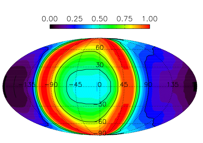
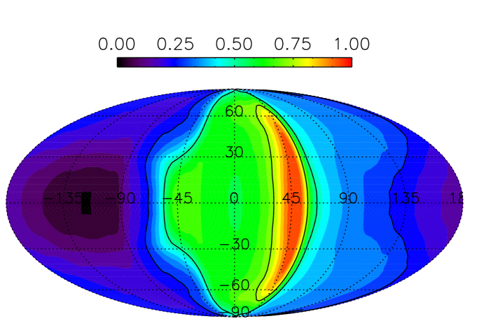
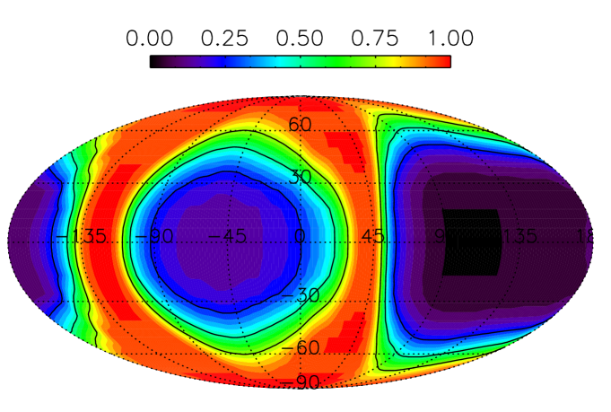
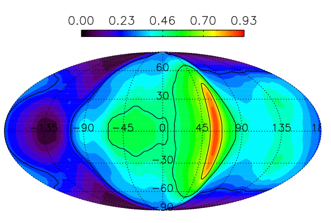
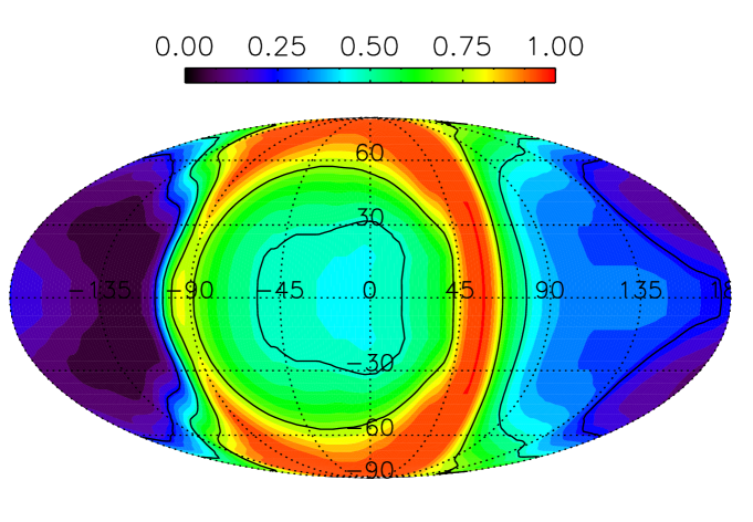
Figure 12.— Anisotropy of the mean accretion intensity (see text), as seen from the center of the planet, projected on Mollweide maps. The longitude $\mp 180^{\circ}$ indicates the direction toward the star and $+90^{\circ}$ is the direction along the orbital motion. An intensity equal to $1$ implies that gas from that direction accretes on the planet, regardless of its place of origin along that line of sight (but within the accretion flow). From top to bottom, the core mass is $5$, $10$, and $15\,\mbox{$M_{\mathrm{E}}$}$. The core is located at $5\,\mbox{AU}$ on the left and at $10\,\mbox{AU}$ on the right.

As anticipated in the previous section, the accretion flow is defined as the gas that crosses the envelope surface and originates from within a distance of $3\mbox{$R_{\mathrm{H}}$}/5$ from the core center. Tracer particles deployed between $R_{e}$ and $3\mbox{$R_{\mathrm{H}}$}/5$ are used to track the motion of the accretion flow. These tracers are either carried inside the envelope or to horse-shoe/circulating orbits of the disk. The accretion flow itself is fed by gas coming from the disk, as clearly shown by the streamlines in the left panels of Figures 9 and 10. It is thus expected that the accretion flow, as seen from the core center, is directionally dependent (as opposed to a strictly spherical accretion).

In order to quantify the anisotropy of the gas accreting on the envelope, we introduce an “accretion intensity” along a given direction, as seen from the center of the planet. Each tracer initially released on a spherical shell exterior to the envelope is assigned an “intensity” of $1$ if it moves inside the envelope. Otherwise, the accretion intensity of the tracer is $0$. For a given direction, we take the mean of the accretion intensities defined on all these spherical shells. This quantity represents a measure of the anisotropy of the accretion flow, but it does not bear information on the mass flux delivered to the planet.

The mean accretion intensity is projected on Mollweide maps in Figure 12. The contours levels on the maps indicate locations where the intensity is $0.25$, $0.5$, and $0.75$. The longitude $0^{\circ}$ is the direction along the core-star line, pointing away from the star. Longitudes $\mp 90^{\circ}$ are, respectively, the directions opposite and along the orbital motion. Each map refers to a core of different mass and semimajor axis (see the figure caption for further details). The scale on these maps is absolute in the sense that an intensity of $1$ ($0$) implies that gas originating from that direction (but inside the accretion flow!) always (never) accretes on the planet, whatever its distance. An intensity of $0.5$ implies that, along that line of sight, gas is equally both accreting and non-accreting. Consequently, the scale on the maps should not necessarily start from $0$ (although it does in Figure 12) or reach $1$, as is the case for the mean accretion intensity around the $10\,\mbox{$M_{\mathrm{E}}$}$ core located at $10\,\mbox{AU}$.

There are some common features on the accretion intensity maps as, for example, the relatively low tendency for gas to accrete along the equator at longitude $\sim 180^{\circ}$ (star-ward direction) and the relatively high tendency to accrete around longitude $+45^{\circ}$. In general, for a given meridian, there is higher tendency for gas to accrete away from the equator, although this trend is less clear around the $10\,\mbox{$M_{\mathrm{E}}$}$ core at $10\,\mbox{AU}$.

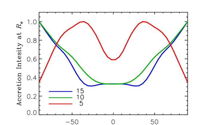
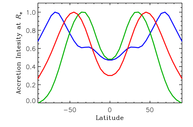
Figure 13.— Normalized intensity of accretion at the envelope surface, integrated in longitude, as a function of the latitude. The curves represent the relative tendency for accreting gas to penetrate the envelope surface. The top and bottom panels refer to planets located at $5$ and $10\,\mbox{AU}$, respectively. The core mass is indicated in the top panel in units of $M_{\mathrm{E}}$.

The maps in Figure 12 provide information about the anisotropy of the accretion flow integrated along the line of sight, that is, the direction from which accreting gas originates. However, they convey no direct information about the angular distribution of the locations where accreting gas actually enters the envelope. Such a distribution can be obtained from the trajectories of the tracers in the accretion flow, as they intersect the sphere of radius $R_{e}$. We count the number of intersections as a function of the latitude, defined as in Figure 12, and constructed an equivalent of the accretion intensity at $R=R_{e}$. The resulting distributions, normalized to their maxima, are plotted in Figure 13. The curves clearly show that gas accreting on the envelope does so preferentially at mid- to high latitudes.

6. Summary and Conclusions

We present detailed and global radiation-hydrodynamics calculations of 3D envelopes around planetary cores embedded in protoplanetary disks. The global approach allows us to fully take into account the circulation of gas as it orbits the star and moves toward the planet. We consider cores of $5$, $10$, and $15\,\mbox{$M_{\mathrm{E}}$}$ at $5$ and $10\,\mbox{AU}$ from a solar-mass star. The equation of state includes both gas and radiation, and gas is treated as a solar mixture of H₂, H, He, and their ions (see Section 2.3). Molecular hydrogen is modeled as a mixture of parahydrogen and orthohydrogen with a fixed $1/3$ ratio. Detailed calculations of dust opacity are also performed, assuming the presence of multiple grain species (see Section 2.4). Nested grids are used to resolve the flow at various length scales, from the orbital to the core radius (see Section 3.2). Some average properties of equilibrium disk structures (see Section 4) are summarized in Table 1. The energy budget of the envelopes accounts for deposition of energy due to solids accretion, obtained from 1D calculations (see Section 5.1).

The masses and gas accretion rates of 1D and 3D envelopes differ by a factor $2$ or less (see Table 2). The density (for $R>3\,R_{c}$) and temperature in the envelope differ by factors smaller than $10$ and $2$, respectively (see Figure 7). The largest differences typically occur at the boundaries of 1D envelopes, whose density and temperature are matched to the azimuthally averaged values of the disk at the corresponding orbital distance (see Figure 3). We find that perturbations induced by the core can raise the local density and temperature above these average disk values. The interior structure of 1D envelopes is not very sensitive to boundary conditions (compare left and right panels in Figure 7). Despite the approximate gravitational potential at $R_{c}$ and limited linear resolution ($\approx R_{c}$) of the 3D calculations, density, temperature, and pressure at $R\approx R_{c}$ are comparable to those of the 1D envelopes in most cases. The general consistency of two very different physical approximations and entirely different numerical solutions represents an important, two-way validation of the 1D and 3D models.

Energy-based arguments (see Section 5) suggest that when $\mbox{$R_{\mathrm{B}}$}<\mbox{$R_{\mathrm{H}}$}$ (as in all the cases studied here), the envelope does not extend beyond the Bondi sphere. The behavior of the gas streamlines around the cores agrees with such a conclusion (see Figures 9 and 10). By means of passive tracers we identify the volume of the gas bound to the core. We obtain envelope radii that increase with core mass, and range from $R_{e}\approx 0.4$ to $\approx 0.9\,\mbox{$R_{\mathrm{B}}$}$ (see Table 3). Marginal variations of $R_{e}$ ($\lesssim 10$%) are obtained between envelopes around cores located at $5$ and $10\,\mbox{AU}$. We find that interactions with the external flow can produce asymmetries (e.g., in temperature) in the outer layers of an envelope.

We determine the moments of inertia and angular momenta of the envelopes and estimate bulk rotation rates using the rigid-body approximation (see Section 5.3). The results indicate slow rotation, consistent with the mean angular velocity of the gas at the equator, between $R_{e}/2$ and $R_{e}$. The oblateness of the envelopes is estimated by using the homogeneous ellipsoid and the hydrostatic equilibrium approximations. Both solutions point to a moderate to low flattening ($\lesssim 0.05$), although the latter method typically provides smaller values than the former. This may suggest that the oblateness is not caused entirely by rotation or that one or both approximations are not accurate enough.

We define an accretion flow in the region between $R_{e}$ and $3\mbox{$R_{\mathrm{H}}$}/5$ and study its directional dependence as seen from the planet center (see Section 5.4). The anisotropy clearly shows that the accretion is not spherical (see Figure 12). We also identify the angular distribution of the locations where the accretion flow enters the envelope (see Figure 13), which displays a tendency toward merging at mid- to high latitudes.

Estimates of the specific angular momentum of Jupiter and Saturn are, respectively, $\approx 2\times 10^{15}$ and $\approx 10^{15}\,\mathrm{cm^{2}\,s^{-1}}$. The envelopes surrounding the $10$ and $15\,\mbox{$M_{\mathrm{E}}$}$ cores at $5\,\mbox{AU}$ have specific angular momenta of order $10^{15}\,\mathrm{cm^{2}\,s^{-1}}$, and $\approx 4\times 10^{14}\,\mathrm{cm^{2}\,s^{-1}}$ for the same cores at $10\,\mbox{AU}$ (see Table 3). These figures also give the specific angular momentum of the gas in the corresponding accretion flows (as defined here). If such planets evolved into Jupiter and Saturn, via continued accretion of gas, the specific angular momentum of the accreted gas should be comparable to that of the gas accreted during these earlier phases of evolution.

Overall, these 3D calculations, applied to relatively low-mass gaseous envelopes around protoplanetary cores, provide a firm basis for the calculation of gas accretion rates onto such cores and for the study of non-spherically symmetric envelope properties. These results indicate that the 3D code can now be extended to the later stages of evolution when the gas accretion rates are high and are limited by the detailed physics of the disk rather than by the thermal properties of the planetary envelope. At present, such accretion rates, which cannot be determined in 1D simulations, are generally simulated in 3D applying a local isothermal equation of state (Lissauer et al., 2009; Bodenheimer et al., 2013). Future simulations should determine the effect on these rates of the radiative feedback of the planet onto the disk. At the later stages, a subdisk is expected to form around the planet. The simulations should be able to estimate the effects of this subdisk on the gas flow onto the planet and whether this flow, as suggested above, carries low specific relative angular momentum (see also Tanigawa et al., 2012; Ayliffe & Bate, 2012). Ultimately, such calculations should be able to determine the final mass and angular momentum of a giant planet, given a set of initial conditions.

Appendix A Dust Opacity Calculation

Let us indicate with $\kappa_{\lambda}$ the monochromatic opacity (absorption plus scattering) coefficient at the radiation wavelength $\lambda$, so that $\tau_{\lambda}=\int{\kappa_{\lambda}\rho dl}$ is the optical thickness of the medium along the direction $l$ at that same wavelength. (Notations used in this Appendix may be unrelated to the same symbols adopted in other parts of the paper.) The equations of radiation hydrodynamics are often applied in a frequency-integrated form, as are Equations (7), (8), and (9). Under the local thermodynamic equilibrium, the frequency-integrated opacity coefficient involved in the radiation flux in Equation (12) is the Rosseland mean opacity, $\kappa_{\mathrm{R}}$, defined by (e.g., Castor, 2007)

$$\frac{1}{\kappa_{\mathrm{R}}}=\frac{\int_{0}^{\infty}{(1/\kappa_{\lambda})(\partial B_{\lambda}/\partial T)d\lambda}}{\int_{0}^{\infty}{(\partial B_{\lambda}/\partial T)d\lambda}},$$ (A1)

where $B_{\lambda}=B_{\lambda}(T)$ is the Planck’s function (see Gray, 1992). Although, not employed in this study, the Planck mean opacity

$$\kappa_{\mathrm{P}}=\frac{\int_{0}^{\infty}{\kappa_{\lambda}B_{\lambda}d\lambda}}{\int_{0}^{\infty}{B_{\lambda}d\lambda}}$$ (A2)

may also be required if, for example, the total radiation flux includes contributions from external irradiation sources (e.g., Rafikov & De Colle, 2006).

If we consider protoplanetary disk regions with densities $\rho\lesssim 10^{-8}\,\mathrm{g\,cm}^{-3}$, the Rosseland mean opacity due to atoms and molecules at temperatures $T\lesssim 1500\,\mbox{$\mathrm{K}$}$ is less than $10^{-3}\,\mathrm{cm^{2}\,g^{-1}}$, and less than $10^{-4}\,\mathrm{cm^{2}\,g^{-1}}$ below $1000\,\mbox{$\mathrm{K}$}$ (e.g., Freedman et al., 2008). At such temperatures, however, dust grains entrained in the gas also contribute to absorption and scattering of radiation. In fact, below $1000\,\mbox{$\mathrm{K}$}$, dust opacity typically dominates by a large margin over gas opacity. In the following, we assume that gas opacity is small compared to dust opacity in the range of temperatures that allows for the presence of dust.

Consider a size distribution so that the number of grains, of radius $a$, of the dust species $i$ is $n^{i}(a)$. Let us indicate the cross-section for absorption and scattering of photons by a dust particle as $\sigma^{i}(a,\lambda)=\pi a^{2}\mathcal{Q}^{i}(a,\lambda)$, where $\mathcal{Q}$ is the total extinction (absorption plus scattering) efficiency of the particle. The opacity coefficient of species $i$, $\kappa^{i}_{\lambda}$, is given by

$$\kappa^{i}_{\lambda}=\frac{f_{s}^{i}\int{n^{i}(a)\sigma^{i}(a,\lambda)da}}{(4\pi/3)\rho_{s}^{i}\int{n^{i}(a)a^{3}da}},$$ (A3)

where $\rho_{s}^{i}$ is the density of the solid grain and $f_{s}^{i}$ is the mass fraction of the solid species, so that its mass per unit volume is $\rho f_{s}^{i}$ ($\rho$ is the gas density). Summing over all grain species, the total monochromatic opacity of the dust is

$$\kappa_{\lambda}=\sum_{i}\kappa^{i}_{\lambda}.$$ (A4)

The grain extinction efficiency, $\mathcal{Q}$, is the sum of the absorption efficiency, $\mathcal{Q}_{\mathrm{ab}}$, and the scattering efficiency $\mathcal{Q}_{\mathrm{sc}}$. Pollack et al. (1985) discusses the presence of a modulation factor that multiplies the extinction efficiency and that accounts for anisotropic scattering, which may be important when the radiation wavelength is comparable to the grain size. Here, this factor is embedded in $\mathcal{Q}$. Since we assume that grains are spherical particles, Mie theory can be applied to compute the extinction efficiency. Let us introduce the ratio $\xi=2\pi a/\lambda$, and the real and imaginary parts of the refraction index of the material, $\mathcal{N}_{r}$ and $\mathcal{N}_{i}$, respectively. If $(\mathcal{N}_{r}-1)\xi\ll 1$, i.e., in the limit of small particles, it can be shown (Pollack et al., 1985) that $\mathcal{Q}_{\mathrm{ab}}\propto\xi$ and $\mathcal{Q}_{\mathrm{sc}}\propto\xi^{4}$, and hence $\mathcal{Q}$ is dominated by absorption. In particular, for small particles the asymptotic form of the absorption efficiency is $\mathcal{Q}_{\mathrm{ab}}\approx 8\mathcal{N}_{r}\mathcal{N}_{i}/[(\mathcal{N}^{2}_{r}-\mathcal{N}^{2}_{i}-2)^{2}+4\mathcal{N}^{2}_{r}\mathcal{N}^{2}_{i}]$ (Pollack et al., 1985). In the limit of large particles, $\xi\gg 1$, one typically finds that $\mathcal{Q}_{\mathrm{ab}}+\mathcal{Q}_{\mathrm{sc}}\approx 1$.

To compute the extinction efficiency of a solid grain we employ the Mie theory according to the formulation of Bohren & Huffman (1983) for homogeneous spheres. We follow Pollack et al. (1994) and consider the dust as mixture of seven grain species, made of iron, olivine, orthopyroxene, troilite (FeS), refractory and volatile organics, and water ice. The material densities, $\rho_{s}$, the mass fractions, $f_{s}$, as well as the representative vaporization temperatures versus gas density are taken from Tables 2 and 3 of Pollack et al. (1994). The combined gas-to-dust mass ratio is $71.5$. The optical properties of the various materials, that is the real and imaginary parts of the refraction index $\mathcal{N}_{r}$ and $\mathcal{N}_{i}$ as a function of wavelength, come from the Database of Optical Constants maintained by the Astrophysical Institute of the University of Jena.

We use the same size distribution for all grain species, given by a simple power-law of the grain radius, $n(a)\propto a^{-3}$. The minimum and maximum radii of the distribution, $0.005\,\mu\mathrm{m}$ and $1\,\mathrm{mm}$, are also the same for all species. Both the power index of the distribution and its maximum radius compare favorably with observations of T Tauri disks, as shown by models of the spectral energy distributions (D’Alessio et al., 2001). In fact, the study of D’Alessio et al. (2001) suggests that grain growth in these disks can lead to distributions containing grains with radii possibly larger than $\sim 1\,\mathrm{cm}$. The size distribution of interstellar grains is typically taken as $n(a)\propto a^{-3.5}$, with radii varying between $0.005$ and $0.25\,\mu\mathrm{m}$ (Draine & Lee, 1984). For comparison purposes, we also compute interstellar opacities applying this size distribution and the composition and mass fractions adopted by Pollack et al. (1994) for molecular clouds.

The integrals in Equation (A3) are performed by means of a “cautious extrapolation” integration based on an adaptive Romberg method (Davis & Rabinowitz, 2007). The convergence of each integration is achieved within a relative error tolerance of $10^{-7}$ or an absolute error tolerance of $10^{-15}$. The monochromatic opacity is calculated with a relative wavelength resolution $d\lambda/\lambda\approx 1.4\times 10^{-4}$. The integration of the Rosseland and Planck opacities, in Equations (A1) and (A2), is performed applying the same integration algorithm and requiring the same precision.

Grain opacities depend on gas density only through the vaporization temperature (Pollack et al., 1994). For temperatures higher than the highest vaporization temperature $T^{\mathrm{mx}}_{\mathrm{ev}}$, grains are considered entirely vaporized and only gas contributes to the opacity of the medium. We use a linear interpolation between the dust opacity discussed here and the gas opacity of Ferguson et al. (2005) (see Section 2.4) in the temperature range $[0.8\,T^{\mathrm{mx}}_{\mathrm{ev}},T^{\mathrm{mx}}_{\mathrm{ev}}]$.

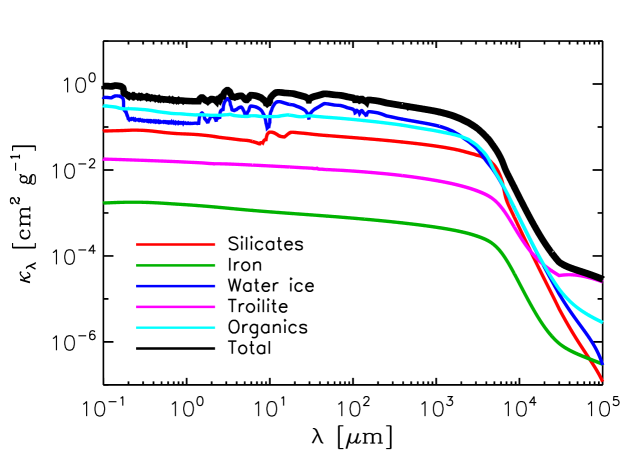
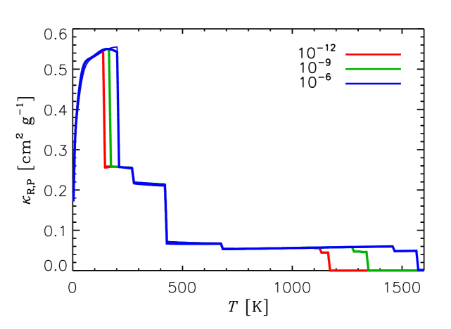
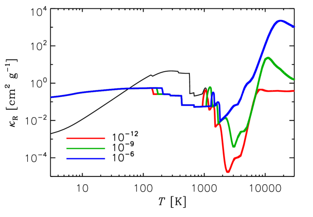
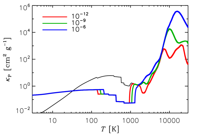
Figure 14.— Top-left: monochromatic opacity (Equation (A3)) as a function of wavelength for the various grain species, as labelled. Olivine and orthopyroxene are grouped under silicates, while organics include both refractory and volatile species. The thick solid line is the sum of the single contributions (Equation (A4)). Top-right: Rosseland (Equation (A1), thicker lines) and Planck mean opacity (Equation (A2), thinner lines) of the dust mixture for three reference gas densities (as indicated in units of $\mathrm{g\,cm}^{-3}$). Bottom: Rosseland (left) and Planck mean opacity (right) of dust and gas, for three reference gas densities (as labelled in units of $\mathrm{g\,cm}^{-3}$). The thin black lines represent the interstellar opacity (see text), assuming a density of $10^{-12}\,\mathrm{g\,cm}^{-3}$.

The top-left panel of Figure 14 shows the monochromatic opacities versus wavelength, $\kappa^{i}_{\lambda}$, of silicates (olivine and orthopyroxene), iron, water ice, troilite, and (refractory and volatile) organics, as indicated. The thicker line is the total monochromatic opacity (Equation (A4)). The Rosseland mean opacity (Equation (A1)) of the dust versus temperature is shown in the top-right panel, for three values of $\rho$, as indicated in the legend in units of $\mathrm{g\,cm}^{-3}$. In the same panel, the Planck mean opacity (Equation (A2)) of the dust is plotted for comparison, showing only minor differences over that range of temperatures. In the bottom panels of the figure, the Rosseland and Planck mean opacity of dust and gas are plotted for the same reference densities (see the figure caption for further details). The bottom panels also show the interstellar opacities (thin curves) computed as explained above. The grain species are the same as in the other opacities, but the mass fractions $f_{s}$ are different (the gas-to-dust mass ratio is $106.5$). At temperature $100\lesssim T\lesssim 1000\,\mbox{$\mathrm{K}$}$, the larger grains used for disk opacity reduce $\kappa_{\mathrm{R}}$ by a factor $\approx 10$ relative to that produced by interstellar grains. Note that the largest disk grains are such that $\xi\gg 1$, and their contribution to $\kappa_{\mathrm{R}}$ is approximately proportional to $1/a$. For $T\ll 1000\,\mbox{$\mathrm{K}$}$, the interstellar grains are such that $\xi\ll 1$ and $\kappa_{\mathrm{R}}$ becomes approximately proportional to some power of $T$ (Pollack et al., 1985).

Appendix B Solution of a Special Quartic Equation

In this Appendix, we first show in a mathematical sense that there is one, and one only, temperature that satisfies Equation (32), and then provide the formal solutions to this equation. We refrain from giving a full derivation of these solutions, as such derivation can be found in many textbooks. We caution the reader that notations used in this Appendix have no connection with the same notations used elsewhere in the paper.

Consider a fourth-order polynomial of the type

$$g(z)=az^{4}+bz-E,$$ (B1)

in which the constants $a$, $b$, and $E$ are non-zero, positive real numbers and the variable $z$ is a real number. By taking the derivative $dg/dz$, one finds that $g$ is an increasing function for $z^{3}>-b/(4a)$, and decreasing otherwise. Since $g(0)=-E<0$ and the minimum has a negative abscissa, the polynomial $g(z)$ has two real roots: one negative and the other positive, which proves the existence of a single physically relevant temperature that satisfies Equation (32). These same conclusions apply if $b=0$.

In order to determine the zeros of $g(z)$, one can proceed by applying Ferrari’s transformations and show that the four roots can be found by solving the two quadratic equations

$$z^{2}-Hz+W+HD/(4W) = 0$$ (B2)

$$z^{2}+Hz+W-HD/(4W) = 0,$$ (B3)

where $D=b/a>0$, $H=\sqrt{2W}$, and $W$ is a real solution of the auxiliary cubic equation

$$8w^{3}+8Cw-D^{2}=0,$$ (B4)

where $C=E/a>0$. Recall that any polynomial of odd degree admits at least one real solution. Notice that $W=0$ is a solution only if $D=0$ (but in this case the solution of Equation (B1) is trivial).

The statement made above regarding the roots of Equation (B2) and (B3) being equal to the roots of Equation (B1) can be readily proved by multiplying the left-hand sides of Equations (B2) and (B3) and then adding and subtracting $C$, which yields $z^{4}+Dz-C+(8W^{3}+8CW-D^{2})/8W$. Therefore, in the non-trivial case $W\neq 0$, the validity of our statement is demonstrated.

Let us introduce the discriminant

$$\Delta=\left(\frac{D}{4}\right)^{4}+\left(\frac{C}{3}\right)^{3},$$ (B5)

and the two quantities

$$A = \left[(D/4)^{2}+\sqrt{\Delta}\right]^{1/3}$$ (B6)

$$B = \left[(D/4)^{2}-\sqrt{\Delta}\right]^{1/3}.$$ (B7)

By applying the method of Cardano-Tartaglia, one can find the three solutions of Equation (B4)

$$w_{1} = (A+B)$$ (B8)

$$w_{2} = -(A+B)/2+\sqrt{-3}(A-B)/2$$ (B9)

$$w_{3} = -(A+B)/2-\sqrt{-3}(A-B)/2.$$ (B10)

Since $C>0$ then $\Delta>0$, hence both $A$ and $B$ are real numbers, and thus $w_{1}$ is a real solution, while $w_{2}$ and $w_{3}$ are complex conjugate solutions. Therefore, we shall identify $W$, in Equations (B2) and (B3), with $w_{1}$.

It is easy to show that the real solution, $W$, is positive. In fact, $A>0$ and $A>|B|$ ($B<0$), from which follows that $W>0$. It is then straightforward to conclude that the two solutions of Equation (B2), $z_{1}$ and $z_{2}$, are complex conjugate, since its discriminant is negative. In addition, since we proved above that the quartic $g(z)$ must have two real solutions of opposite sign, the roots of Equation (B3), $z_{3}$ and $z_{4}$, must be real. The positive solution of Equation (B1) is therefore

$$z_{4}=\frac{1}{2}\left(\sqrt{HD/W-H^{2}}-H\right).$$ (B11)

Alternatively, one can directly prove $z_{4}$ in Equation (B11) to be positive by showing that the inequality $HD/W-H^{2}>H^{2}$ is always true. We recall that $D=b/a$ and $H=\sqrt{2W}$ and $W$ is given by Equation (B8). The inequality holds if $W^{3}<2(D/4)^{2}$. From Equation (B5), we know that $\Delta>(D/4)^{4}$ and $B<0$, and thus $A>-B>0$. Therefore, we have $W^{3}=A^{3}+B^{3}+3AB(A+B)=2(D/4)^{2}+3AB(A+B)$ with $AB<0$ and $A+B>0$, hence $W^{3}<2(D/4)^{2}$.

Appendix C Tests of the Radiation Flux-Limited Diffusion Solver

In this Appendix, we present some tests of the radiation flux-limited diffusion solver discussed in Section 3.1. As in the previous Appendices, the notations used here have no relation to those used in other parts of the paper.

The first case we shall consider is that of the 1D heat diffusion equation with a constant diffusion coefficient $\mathcal{K}$

$$\frac{\partial U}{\partial t}=\mathcal{K}\frac{\partial^{2}{U}}{\partial z^{2}},$$ (C1)

and initial condition $U(z,0)=U_{0}\delta(z-z_{0})$, whose solution is the well-known heat kernel

$$U(z,t)=\frac{U_{0}}{\sqrt{4\pi\mathcal{K}t}}e^{-(z-z_{0})^{2}/(4\mathcal{K}t)}$$ (C2)

Figure 15.— Left: diffusion of an initial “pulse” represented by the Dirac $\delta$-function, $\delta(z)$. The top part of the panel shows numerical and analytical solutions of Equation (C1), respectively represented (but not distinguishable) by thick and thin lines, at various times in arbitrary units as indicated. The difference between numerical and analytical solution, normalized to the analytical solution, is plotted in the bottom part of the panel. Right: as in the left panel, but for a “three-pulse” initial condition proportional to $\delta(z+0.04)-\delta(z)+\delta(z-0.04)$.

The numerical solution of Equation (C1), for the initial condition $U(z,0)\propto\delta(z)$, is plotted in the left panel of Figure 15 (thick lines) at various times (in arbitrary units), as indicated in the legend. The analytic solution (Equation (C2)) is overlaid (as thin lines) to the numerical solution. Here, and in the other tests presented in this Appendix, analytic and numerical results are indistinguishable on the plot scale. At the bottom of the panel, we also plot the normalized difference $\Delta U/U$ between the numerical and analytical solutions. Obviously, any linear combination of functions of the type in Equation (C2) is also a solution of Equation (C1). The right panel of Figure 15 shows the evolution of an initial condition $U(z,0)\propto[\delta(z+0.04)-\delta(z)+\delta(z-0.04)]$. As in the left panel, we plot the numerical and analytical solution (top), as well as the normalized difference $\Delta U/U$ (bottom). In both calculations, the time step is set equal to $4000$ in units of $(\Delta z)^{2}/\mathcal{K}$.

Let us now consider the more general diffusion equation

$$\frac{\partial U}{\partial t}=\nabla\!\boldsymbol{\cdot}\!{(\mathcal{K}\nabla{U})},$$ (C3)

in which $U=U(t,r,\theta,\phi)$. We aim at deriving simple analytic solutions to this equation using separation of variables and making appropriate assumptions on the diffusion coefficient, $\mathcal{K}$.

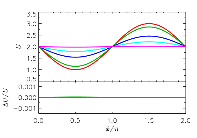
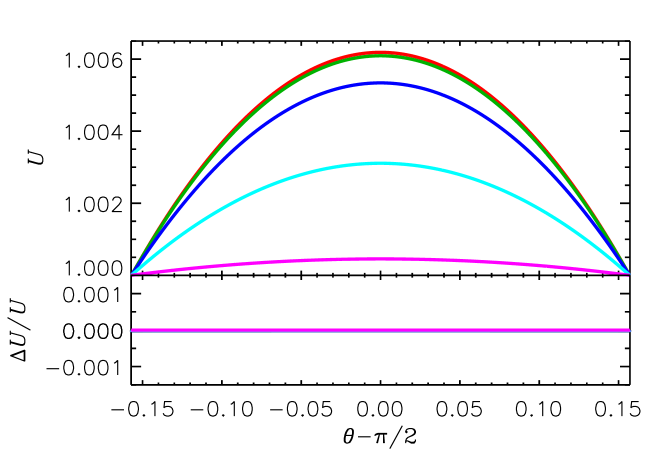
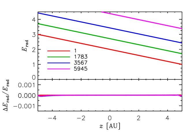
Figure 16.— Comparison between numerical and analytical solutions of Equation (C4) (top-left), (C7) (top-right), (C8) (bottom-left), and (C12) (bottom-right). Although not distinguishable, numerical solutions are plotted as thick lines and analytical solutions as thin lines. In the bottom-left panel, the function $U$ is normalized to its value at $\theta_{\mathrm{min}}$, and plotted at a fixed $r$. In the bottom-right panel, $E_{\mathrm{rad}}$ is normalized to $\bar{E}_{\mathrm{rad}}$ and the labels indicate the time in seconds. The difference between numerical and analytical solution, normalized to the analytical solution, is plotted in the bottom part of each panel.

The first assumption we shall make is that $U$ is isotropic, i.e., $U=U(t,r)$. Equation (C3) is then

$$\frac{\partial U}{\partial t}=\frac{1}{r^{2}}\frac{\partial}{\partial r}\left(r^{2}\mathcal{K}\frac{\partial U}{\partial r}\right).$$ (C4)

If we write $\mathcal{K}=r^{2}_{0}/\tau$, with both $r_{0}$ and $\tau$ constants and assume the existence of solutions of the form $U(t,r)=T(t)R(r)$, Equation (C4) reduces to

$$\left(\frac{\tau}{T}\right)\frac{dT}{dt} = -\xi^{2}$$ (C5)

$$\left(\frac{r^{2}_{0}}{R}\right)\frac{d^{2}R}{dr^{2}}+2\left(\frac{r^{2}_{0}}{rR}\right)\frac{dR}{dr} = -\xi^{2},$$ (C6)

where $\xi$ is a real number. The solution of Equation (C5) is $T(t)=T_{0}e^{-\xi^{2}t/\tau}$. Solutions to the second order differential equation can be found with standard techniques, one of them is $R(r)=(R_{0}/r)\cos{(\xi r/r_{0})}$. Hence, $U(t,r)=T_{0}R_{0}e^{-\xi^{2}t/\tau}\cos{(\xi r/r_{0})}/r$ is solution to Equation (C4). The diffusion coefficient need not be constant. In fact, if $\mathcal{K}=r^{2}/\tau$, a similar approach leads to the solution $U(t,r)=T_{0}e^{-2t/\tau}(c_{1}r+c_{0})/r^{2}$, where $c_{0}$ and $c_{1}$ are integration constants.

The same technique can be applied to look for solutions of the type $U=U(t,\phi)$, which satisfy

$$\frac{\partial U}{\partial t}=\frac{1}{r\sin{\theta}}\frac{\partial}{\partial\phi}\left(\frac{\mathcal{K}}{r\sin{\theta}}\frac{\partial U}{\partial\phi}\right).$$ (C7)

If $\mathcal{K}=(r\sin{\theta})^{2}/\tau$ and $U(t,\phi)=T(t)\Phi(\phi)$, then one can easily show that $U(t,\phi)=T_{0}\Phi_{0}e^{-\xi^{2}t/\tau}\cos{(\xi\phi)}$ is a solution of Equation (C7).

The diffusion equation

$$\frac{\partial U}{\partial t}=\frac{1}{r^{2}}\frac{\partial}{\partial r}\left(r^{2}\mathcal{K}\frac{\partial U}{\partial r}\right)+\frac{1}{r\sin{\theta}}\frac{\partial}{\partial\theta}\left(\frac{\sin{\theta}}{r}\mathcal{K}\frac{\partial U}{\partial\theta}\right)$$ (C8)

can also be solved assuming a diffusion coefficient of the form $\mathcal{K}=r^{2}/(\tau\sin{\theta}$) and expressing the solution as $U(t,r,\theta)=T(t)R(r)\Theta(\theta)$. A solution for the temporal part is again $T(t)=T_{0}e^{-\xi^{2}t/\tau}$. The radial and angular parts can be found by solving the two differential equations

$$\frac{d}{dr}\left(r^{4}\frac{dR}{dr}\right)+\beta^{2}r^{2}R = 0$$ (C9)

$$\frac{d^{2}\Theta}{d\theta^{2}}+(\xi^{2}\sin{\theta}-\beta^{2})\Theta = 0,$$ (C10)

where $\beta^{2}$ is a real number, which for simplicity we set equal to $2$. In such case, as mentioned earlier, a solution to Equation (C9) is $(c_{1}r+c_{0})/r^{2}$. Equation (C10) is a linear differential equation with a transcendental function as coefficient, the solution of which does not typically have a compact form. By expanding the coefficient $\xi^{2}\sin{\theta}-2$ in a Taylor series around $\theta=\pi/2$ and expressing the solution as $\Theta=\sum_{0}^{\infty}{a_{n}\vartheta^{n}}$, where $\vartheta=\pi/2-\theta$, we can determine the coefficients $a_{n}$ of the series from Equation (C10). For symmetry reasons, $\Theta$ is an even function and therefore the series has only even terms. After some tedious algebra, one can write the solution as

$$\Theta(\vartheta)=1+(2-\xi^{2})\vartheta^{2}/2+[(2-\xi^{2})^{2}+\xi^{2}]\vartheta^{4}/24+[(2-\xi^{2})^{3}+7\xi^{2}(2-\xi^{2})-\xi^{2}]\vartheta^{6}/720+\mathcal{O}(\vartheta^{8}).$$ (C11)

A comparison between the analytical solutions presented here and numerical solutions is carried out in Figure 16. The top-left, top-right, and bottom-left panels show, respectively, comparisons for the solutions of Equation (C4), (C7), and (C8). Numerical results are plotted as thick lines, whereas analytical results are plotted as thin lines. The normalized difference between numerical and analytical solution is plotted at the bottom of each panel (see the figure caption for further details). The time step of the three calculations is between $100$ and $500$ in units of $(\Delta S)^{2}/\mathcal{K}$, where $\Delta S$ is $\Delta r$, $r\Delta\theta$, or $r\sin{\theta}\Delta\phi$ (for values of $r$ and $\sin{\theta}\approx 1$).

The solutions presented above apply to diffusion problems. Let us consider the equation

$$\frac{\partial E_{\mathrm{rad}}}{\partial t}=-\nabla\!\boldsymbol{\cdot}\!{\boldsymbol{F}}.$$ (C12)

As mentioned in Section 2.2, in very optically thin media, radiation transfer reaches the streaming limit for which the flux-limiter in Equation (14) is $\lambda=\rho\kappa E_{\mathrm{rad}}/|\nabla{E_{\mathrm{rad}}}|\ll 1$ (which requires the condition $|\nabla{E_{\mathrm{rad}}}|\neq 0$) and the frequency-integrated radiation flux reduces to $\boldsymbol{F}=-\boldsymbol{n}cE_{\mathrm{rad}}$, where $\boldsymbol{n}=\nabla{E_{\mathrm{rad}}}/|\nabla{E_{\mathrm{rad}}}|$. Therefore, in a 1D problem (or along the direction $\boldsymbol{n}$), Equation (C12) becomes a first-order wave or transport equation

$$\frac{\partial E_{\mathrm{rad}}}{\partial t}=c\left|\frac{\partial E_{\mathrm{rad}}}{\partial z}\right|,$$ (C13)

in which $z$ is a linear coordinate, e.g., the cylindrical coordinate parallel to the disk’s axis. It is trivial to conclude that any function $U=U(z\pm ct)$ is a solution to Equation (C13). The sign in the argument is equal to the sign of $\partial E_{\mathrm{rad}}/\partial z$. For the sake of simplicity, let us consider the solution $E_{\mathrm{rad}}=\bar{E}_{\mathrm{rad}}(ct-z+2)$, where $\bar{E}_{\mathrm{rad}}$ is a constant, which is an oblique front that propagates along the $z$-direction at speed $c$. The numerical solution (thick lines) of Equation (C12) is compared to the analytic solution (thin lines) of Equation (C13) in the bottom-right panel of Figure 16. The plot shows the ratio $E_{\mathrm{rad}}/\bar{E}_{\mathrm{rad}}$ versus $z$ at different times, indicated in the legend in seconds, and the relative difference of numerical and analytic solutions at the bottom.

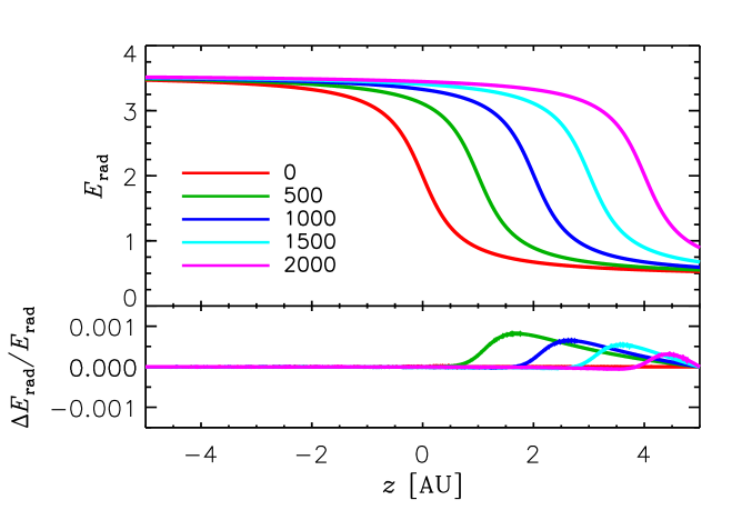
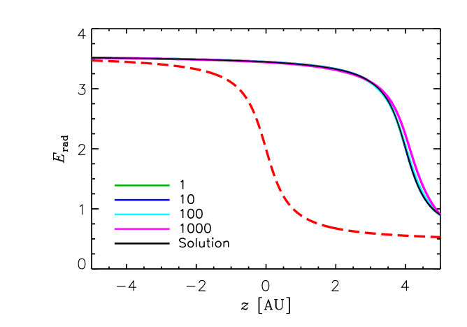
Figure 17.— Left: as in the bottom-right panel of Figure 16, but for the propagation of a sharper front and a calculation with time step equal to $(\Delta t)_{\mathrm{CFL}}$, the maximum allowed for stability of an explicit numerical solution of Equation (C13). The legend gives the times in seconds. Numerical and analytical solutions are plotted, respectively, as thick and thin lines. Right: comparison of implicit numerical solutions of Equation (C13) with the analytic solution, at a given time, for various applied time steps, as indicated in units of $(\Delta t)_{\mathrm{CFL}}$. The dashed line reproduces the front at $t=0$.

In order to test the stability of the flux-limited approach in the streaming limit, when the time step is longer than $(\Delta t)_{\mathrm{CFL}}$ (see Section 3), we follow Turner & Stone (2001), who simulated the propagation of a sharp front, represented by a step function, at the speed of light. A step function is solution to Equation (C13), but $|\nabla{E_{\mathrm{rad}}}|=0$ for $x\neq ct$ so that $\lambda$ in Equation (14) tends to $1/3$ almost anywhere and Equation (C12) remains a diffusion rather than a first-order wave equation. Instead, we choose a propagating front of the type $\arctan{[(ct-z)/10]}$ (plus a constant). In case of Equation (C13), the Courant-Friedrichs-Lewy limiting time step allowed for stability is $(\Delta t)_{\mathrm{CFL}}=\Delta z/(2c)$. In the left panel of Figure 17, we compare the evolution of the front, obtained by solving Equation (C12), with the analytic solution (top), and show the relative difference at the bottom, for a calculation with a time step $\Delta t=(\Delta t)_{\mathrm{CFL}}$ (see the figure caption for details). In the right panel, we compare the numerical and analytical solutions at a given time, for time steps of various lengths, in units of $(\Delta t)_{\mathrm{CFL}}$, as indicated. Since the aim here is to test the stability of the numerical solution rather than the accuracy of the flux-limited diffusion approximation of radiative transfer, in the test reported in right panel of Figure 17 (and in this only!) the ratio $\mathcal{R}$ used to construct in the flux-limiter $\lambda$ (Equation (14)) is computed using the analytic solution.

Figure 18.— Comparisons between numerical and analytical solutions of the radiative diffusion problems, as proposed by Boss (2009) (see text). The upper panels show $E_{\mathrm{rad}}$, divided by the constant $\bar{E}_{\mathrm{rad}}$, for $\rho=10^{-10}\,\mathrm{g\,cm^{-3}}$ and $\kappa=1$ and $0.01\,\mathrm{cm^{2}\,g^{-1}}$. All calculations are initiated with a uniform radiation energy density $E_{\mathrm{rad}}=\bar{E}_{\mathrm{rad}}$. Numerical results are indicated with thick lines and analytical results with thin lines (not distinguishable). The lower panels show the relative difference between numerical and analytical solutions.

Stationary solutions to the radiation diffusion problem for a disk in spherical polar coordinates were published by Boss (2009), who sought special solutions of the equation

$$\frac{1}{3}\frac{c}{\kappa\rho}\nabla^{2}{E_{\mathrm{rad}}}+\varepsilon=0,$$ (C14)

in which $\kappa$ and $\rho$ are constants. The quantity $\varepsilon$ is an energy input rate per unit volume. In particular, he provided a solution for the isotropic case, $E_{\mathrm{rad}}=E_{\mathrm{rad}}(r)$, and a solution for the vertically stratified case, $E_{\mathrm{rad}}=E_{\mathrm{rad}}(\theta)$. One can easily prove that if $\varepsilon=2c\bar{E}_{\mathrm{rad}}/(\kappa\rho\bar{r}^{2})$, $E_{\mathrm{rad}}=\bar{E}_{\mathrm{rad}}[2-(r/\bar{r})^{2}]$ is a solution to Equation (C14), with $\bar{E}_{\mathrm{rad}}$ and $\bar{r}$ constants of integration. Similarly, by setting $\varepsilon=-c\bar{E}_{\mathrm{rad}}\cos{(2\theta)}/(3\kappa\rho r^{2}\sin{\theta})$, then $E_{\mathrm{rad}}=\bar{E}_{\mathrm{rad}}\sin{\theta}$ is a solution of Equation (C14).

We compare numerical solutions of Equation (C14) with the analytic solution of Boss (2009) in Figure 18. We use a density $\rho=10^{-10}\,\mathrm{g\,cm^{-3}}$ and opacities $\kappa=1$ and $0.01\,\mathrm{cm^{2}\,g^{-1}}$. Left and right panels refer to comparisons for the radial and the vertical solutions. The upper panels show the ratio $E_{\mathrm{rad}}/\bar{E}_{\mathrm{rad}}$, while the lower panels show the relative differences of numerical and analytical solutions. These calculations, which use the flux-limiter in Equation (14), indicate that $\lambda$ correctly converges to the diffusion limit (i.e., $1/3$) for such tests.

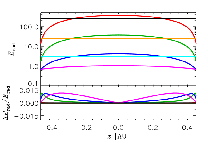
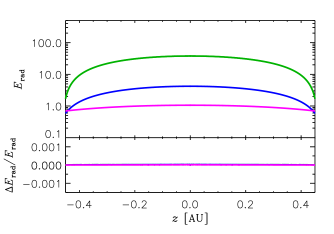
Figure 19.— Left: relaxation test (see Boley et al., 2007a) in which a plane-parallel disk is heated at a constant rate, and opacity and density are constant. In the top of the panel, $E_{\mathrm{rad}}$ calculated numerically and divided by $(4\sigma_{\mathrm{SB}}/c)T^{4}_{\mathrm{eff}}$ (thick lines) is plotted together with its analytic expression (thin line), for $T_{\mathrm{eff}}=100\,\mbox{$\mathrm{K}$}$ and $\tau_{M}=1000$, $100$, $10$, $1$ (upper to lower curved line), $0.1$, $0.01$, $0.001$ (lower to upper straight line). The bottom of the panel shows, for each value of $\tau_{M}$, the difference between computed and analytic result divided by the analytic result. Right: as in the left panel, but only for $\tau_{M}=100$, $10$, $1$ (upper to lower curve) and using the flux-limiter in Equation (C18).

We also perform the “relaxation” test proposed by Boley et al. (2007a), in which a disk with no density stratification is heated at a constant rate per unit volume, $\varepsilon$. We assume a plane-parallel disk in a cylindrical geometry $(z,r,\phi)$, with constant properties in $r$ and $\phi$. For the disk to be stationary,

$$\frac{1}{3}\frac{c}{\kappa\rho}\frac{d^{2}E_{\mathrm{rad}}}{dz^{2}}+\varepsilon=0,$$ (C15)

where the input energy rate per unit volume is

$$\varepsilon=\sigma_{\mathrm{SB}}T^{4}_{\mathrm{eff}}\left(\frac{\kappa\rho}{\tau_{M}}\right).$$ (C16)

In the equations above, both the opacity $\kappa$ and the density $\rho$ are constant, and $\tau_{M}\gtrsim 1$ is the optical depth at the disk mid-plane (the total optical thickness of the disk is $2\tau_{M}$). The radiation flux emitted at the disk surface, $\sigma_{\mathrm{SB}}T^{4}_{\mathrm{eff}}$, is expressed through an effective temperature, $T_{\mathrm{eff}}$.

Equation (C15) is strictly valid in the diffusion limit. By integrating, we find that

$$E_{\mathrm{rad}}=\left(\frac{3\sigma_{\mathrm{SB}}}{c}\right)T^{4}_{\mathrm{eff}}\left[\tau\left(1-\frac{\tau}{2\tau_{M}}\right)+\frac{1}{\sqrt{3}}+\frac{1}{3\tau_{M}}\right],$$ (C17)

in which $z\in[-z_{M},z_{M}]$ is the vertical coordinate ($z=0$ is the disk mid-plane), $\tau=\kappa\rho|z_{M}-z|$, and $\tau_{M}=\kappa\rho z_{M}$. The constants of integration are chosen so that Equation (C17) agrees with the derivation of the temperature stratification given by Hubeny (1990). If $\tau_{M}\gg 1$, the radiation energy density is $E_{\mathrm{rad}}\sim(3\sigma_{\mathrm{SB}}/c)T^{4}_{\mathrm{eff}}(\tau+1/\sqrt{3})$. In the streaming limit, Equation (C15) reduces to $dE_{\mathrm{rad}}/dz=\varepsilon/c$. By choosing appropriately the constant of integration, the solution can be written as $E_{\mathrm{rad}}\sim(3\sigma_{\mathrm{SB}}/c)T^{4}_{\mathrm{eff}}[(\tau+1)/(3\tau_{M})+1/\sqrt{3}]$. For $\tau<\tau_{M}\ll 1$, $E_{\mathrm{rad}}\sim(3\sigma_{\mathrm{SB}}/c)T^{4}_{\mathrm{eff}}[1/\sqrt{3}+1/(3\tau_{M})]$, which is the same as the formal solution of Equation (C17) in the optically thin limit.

Results from comparisons between numerical and analytical solutions of the relaxation problem are reported in Figure 19. The upper part of the left panel shows the ratio $E_{\mathrm{rad}}/[(4\sigma_{\mathrm{SB}}/c)T^{4}_{\mathrm{eff}}]$ for $T_{\mathrm{eff}}=100\,\mbox{$\mathrm{K}$}$ and $\tau_{M}$ ranging from $0.001$ to $1000$. The lower part of the panel shows the normalized difference between numerical and analytic solutions. All calculations are initiated with a uniform radiation field $E_{\mathrm{rad}}=(4\sigma_{\mathrm{SB}}/c)T^{4}_{\mathrm{eff}}$.

For these stationary problems, the flux-limiter in Equation (14) reproduces reasonably well the transition between diffusion and streaming limits. It ought to be stressed, however, that the $\approx 1$% discrepancy, observed at low optical depths for the cases with $\tau_{M}=1$, $10$, and $100$ (see lower-left panel of Figure 19), is not due to inaccuracies or limitations of the numerical solver, but rather to the way the flux-limiter $\lambda$ in Equation (14) transitions from the diffusion to the streaming limit. In fact, using the flux-limiter (Levermore, 1984; Castor, 2007)

$$\lambda=\frac{1}{\max{(3,\mathcal{R})}},$$ (C18)

which provides a sharper transition (at larger $\mathcal{R}$), results in a much better agreement between numerical and analytical solutions for those values of $\tau_{M}$, as can be clearly seen in the right panel of Figure 19. (This flux-limiter is not generally recommended, tough, see Levermore, 1984).

Finally, we comment on the impact of applying a preconditioner (see Section 3.1) to the iterative solvers. In the tests reported here, for which the accuracy of the global convergence criterion (see discussion in Section 3.1) can be independently assessed via comparison with the true solution, the use of the ILU preconditioner results in a reduction of the iteration count of factors between $20$ and $\gtrsim 200$. In the actual calculations, where the problem is much larger and rather more challenging, the reduction of the iteration count is typically smaller, but still substantial (factors $>10$). More importantly, the ILU pre-conditioned system (Section 3.1) generally converges in situations where the non-conditioned system fails to converge.

Appendix D Piecewise Approximation of the Core’s Gravitational Potential

The gravitational potential of a point-mass, $M_{c}$, the planetary core, introduces a singularity on the computational grid at the vector location of the core, $\boldsymbol{r}_{c}$. In disk-planet interaction calculations, this singularity is typically avoided by regularizing the potential, $\Phi_{c}$, so that $\Phi_{c}=-G\mbox{$M_{c}$}/\sqrt{R^{2}+\epsilon^{2}}$, where $\boldsymbol{R}=\boldsymbol{r}-\boldsymbol{r}_{c}$ and $\epsilon$ is a softening length. Clearly, if $\epsilon$ is small enough, for all practical purposes this potential is very similar to the true potential (almost) everywhere on the grid.

More sophisticated approximations, using piecewise reconstructions of the true potential, have also been introduced (e.g., Klahr & Kley, 2006; Kley et al., 2009). These functional forms have the property of becoming the true potential, beyond some distance from the point-mass. In the calculations presented in this paper, we follow this sophisticated approach and introduce a piecewise reconstruction of the core’s potential that involves fifth-order polynomials

$$\Phi_{c}=\left\{\begin{array}[]{l l}\left[\frac{1}{10}\left(R/\epsilon\right)^{5}-\frac{3}{10}\left(R/\epsilon\right)^{4}+\frac{2}{3}\left(R/\epsilon\right)^{2}-\frac{14}{10}\right]\left(G\mbox{$M_{c}$}/\epsilon\right)&\mathrm{if}\quad R/\epsilon\leq 1\\ &\\ \left[-\frac{1}{30}\left(R/\epsilon\right)^{5}+\frac{3}{10}\left(R/\epsilon\right)^{4}-\left(R/\epsilon\right)^{3}+\frac{4}{3}\left(R/\epsilon\right)^{2}-\frac{16}{10}\right]\left(G\mbox{$M_{c}$}/\epsilon\right)+\frac{1}{15}G\mbox{$M_{c}$}/R&\mathrm{if}\quad 1<R/\epsilon\leq 2\\ &\\ -G\mbox{$M_{c}$}/R&\mathrm{otherwise}.\end{array}\right.$$ (D1)

We set the length $\epsilon$ between $1$ and $2$ core radii, $R_{c}$, basically on the order of the linear resolution on the finest gird level. Equation (D1) is applied to all grids with the same value of $\epsilon$. Therefore, an exact potential is effectively used over the entire grid domain, on all but the top-most grid level.

References

- Asplund et al. (2009) Asplund, M., Grevesse, N., Sauval, A. J., & Scott, P. 2009, ARA&A, 47, 481
- Ayliffe & Bate (2009) Ayliffe, B. A., & Bate, M. R. 2009, MNRAS, 393, 49
- Ayliffe & Bate (2012) Ayliffe, B. A., & Bate, M. R. 2012, MNRAS, 427, 2597
- Bate et al. (2003) Bate, M. R., Lubow, S. H., Ogilvie, G. I., & Miller, K. A. 2003, MNRAS, 341, 213
- Black & Bodenheimer (1975) Black, D. C., & Bodenheimer, P. 1975, ApJ, 199, 619
- Bodenheimer et al. (2013) Bodenheimer, P., D’Angelo, G., Lissauer, J. J., Fortney, J. J., & Saumon, D. 2013, ApJ, 770, 120
- Bodenheimer & Pollack (1986) Bodenheimer, P., & Pollack, J. B. 1986, Icarus, 67, 391
- Bohren & Huffman (1983) Bohren, C. F., & Huffman, D. R. 1983, Absorption and Scattering of Light by Small Particles (New York: Wiley)
- Boley et al. (2007a) Boley, A. C., Durisen, R. H., Nordlund, Å., & Lord, J. 2007a, ApJ, 665, 1254
- Boley et al. (2007b) Boley, A. C., Hartquist, T. W., Durisen, R. H., & Michael, S. 2007b, ApJ, 656, L89
- Boss (2009) Boss, A. P. 2009, ApJ, 694, 107
- Britz et al. (2003) Britz, D., Østerby, O., & Strutwolf, J. 2003, Computational Biology and Chemistry, 27, 253
- Castor (2007) Castor, J. I. 2007, Radiation Hydrodynamics (Cambridge: Cambridge University Press)
- Chandrasekhar (1967) Chandrasekhar, S. 1967, Communications on Pure and Applied Mathematics, 20, 251
- Cook (2009) Cook, A. H. 2009, Interiors of the Planets (Cambridge: Cambridge University Press)
- D’Alessio et al. (2001) D’Alessio, P., Calvet, N., & Hartmann, L. 2001, ApJ, 553, 321
- D’Angelo et al. (2005) D’Angelo, G., Bate, M. R., & Lubow, S. H. 2005, MNRAS, 358, 316
- D’Angelo et al. (2002) D’Angelo, G., Henning, T., & Kley, W. 2002, A&A, 385, 647
- D’Angelo et al. (2003a) D’Angelo, G., Henning, T., & Kley, W. 2003a, ApJ, 599, 548
- D’Angelo et al. (2003b) D’Angelo, G., Kley, W., & Henning, T. 2003b, ApJ, 586, 540
- D’Angelo & Lubow (2008) D’Angelo, G., & Lubow, S. H. 2008, ApJ, 685, 560
- D’Angelo & Lubow (2010) D’Angelo, G., & Lubow, S. H. 2010, ApJ, 724, 730
- D’Angelo & Marzari (2012) D’Angelo, G., & Marzari, F. 2012, ApJ, 757, 50
- Davis & Rabinowitz (2007) Davis, P. J., & Rabinowitz, P. 2007, Methods of Numerical Integration (New York: Dover)
- Davis (2005) Davis, S. S. 2005, ApJ, 627, L153
- de Val-Borro et al. (2006) de Val-Borro, M., Edgar, R. G., Artymowicz, P., Ciecielag, P., Cresswell, P., D’Angelo, G., Delgado-Donate, E. J., Dirksen, G., Fromang, S., Gawryszczak, A., Klahr, H., Kley, W., Lyra, W., Masset, F., Mellema, G., Nelson, R. P., Paardekooper, S., Peplinski, A., Pierens, A., Plewa, T., Rice, K., Schäfer, C., & Speith, R. 2006, MNRAS, 370, 529
- DeCampli et al. (1978) DeCampli, W. M., Cameron, A. G. W., Bodenheimer, P., & Black, D. C. 1978, ApJ, 223, 854
- Demmel et al. (2000) Demmel, J., Koev, P., & Li, X. 2000, A Brief Survey of Direct Linear Solvers, ed. Z. Bai, J. Demmel, J. Dongarra, A. Ruhe, & H. van der Vorst (Philadelphia, PA: Society for Industrial and Applied Mathematics), 326–331
- Draine (2011) Draine, B. T. 2011, Physics of the Interstellar and Intergalactic Medium (Princeton, NJ: Princeton University Press)
- Draine & Lee (1984) Draine, B. T., & Lee, H. M. 1984, ApJ, 285, 89
- Ferguson et al. (2005) Ferguson, J. W., Alexander, D. R., Allard, F., Barman, T., Bodnarik, J. G., Hauschildt, P. H., Heffner-Wong, A., & Tamanai, A. 2005, ApJ, 623, 585
- Freedman et al. (2008) Freedman, R. S., Marley, M. S., & Lodders, K. 2008, ApJS, 174, 504
- Gray (1992) Gray, D. F. 1992, The Observation and Analysis of Stellar Photospheres (Cambridge: Cambridge University Press)
- Grevesse & Sauval (1998) Grevesse, N., & Sauval, A. J. 1998, Space Sci. Rev., 85, 161
- Gutknecht (2006) Gutknecht, M. 2006, Block Krylov Space Methods for Linear Systems with Multiple Right-Hand Sides: An Introduction (Zurich, Switzerland: ETH-Zurich)
- Hansen et al. (2004) Hansen, C. J., Kawaler, S. D., & Trimble, V. 2004, Stellar Interiors: Physical Principles, Structure, and Evolution (New York: Springer)
- Hubeny (1990) Hubeny, I. 1990, ApJ, 351, 632
- Hubickyj et al. (2005) Hubickyj, O., Bodenheimer, P., & Lissauer, J. J. 2005, Icarus, 179, 415
- Kippenhahn et al. (2013) Kippenhahn, R., Weigert, A., & Weiss, A. 2013, Stellar Structure and Evolution (Berlin: Springer)
- Kittel (2004) Kittel, C. 2004, Elementary Statistical Physics (New York: Dover)
- Klahr & Kley (2006) Klahr, H., & Kley, W. 2006, A&A, 445, 747
- Kley et al. (2009) Kley, W., Bitsch, B., & Klahr, H. 2009, A&A, 506, 971
- Kopal (1978) Kopal, Z., ed. 1978, Dynamics of Close Binary Systems (Dordrecht: Reidel)
- Kowalski (2006) Kowalski, P. M. 2006, ApJ, 641, 488
- Landau & Lifshitz (1976) Landau, L. D., & Lifshitz, E. M. 1976, Course of Theoretical Physics: Mechanics (Oxford: Pergamon Press)
- Levermore (1984) Levermore, C. D. 1984, J. Quant. Spec. Radiat. Transf., 31, 149
- Levermore & Pomraning (1981) Levermore, C. D., & Pomraning, G. C. 1981, ApJ, 248, 321
- Lissauer (1987) Lissauer, J. J. 1987, Icarus, 69, 249
- Lissauer et al. (2009) Lissauer, J. J., Hubickyj, O., D’Angelo, G., & Bodenheimer, P. 2009, Icarus, 199, 338
- Lodders (2010) Lodders, K. 2010, in Principles and Perspectives in Cosmochemistry, ed. A. Goswami & B. E. Reddy (Berlin: Springer), 379
- Masset et al. (2006) Masset, F. S., D’Angelo, G., & Kley, W. 2006, ApJ, 652, 730
- Mihalas & Weibel Mihalas (1999) Mihalas, D., & Weibel Mihalas, B. 1999, Foundations of Radiation Hydrodynamics (New York: Dover)
- Movshovitz et al. (2010) Movshovitz, N., Bodenheimer, P., Podolak, M., & Lissauer, J. J. 2010, Icarus, 209, 616
- Murray & Dermott (2000) Murray, C. D., & Dermott, S. F. 2000, Solar System Dynamics (Cambridge: Cambridge University Press)
- Nelson & Ruffert (2013) Nelson, A. F., & Ruffert, M. 2013, MNRAS, 429, 1791
- Paardekooper & Mellema (2006) Paardekooper, S.-J., & Mellema, G. 2006, A&A, 459, L17
- Paczyński (1971) Paczyński, B. 1971, ARA&A, 9, 183
- Pathria & Beale (2011) Pathria, R. K., & Beale, P. D. 2011, Statistical Mechanics (Amsterdam: Elsevier)
- Podolak (2003) Podolak, M. 2003, Icarus, 165, 428
- Pollack et al. (1994) Pollack, J. B., Hollenbach, D., Beckwith, S., Simonelli, D. P., Roush, T., & Fong, W. 1994, ApJ, 421, 615
- Pollack et al. (1996) Pollack, J. B., Hubickyj, O., Bodenheimer, P., Lissauer, J. J., Podolak, M., & Greenzweig, Y. 1996, Icarus, 124, 62
- Pollack et al. (1985) Pollack, J. B., McKay, C. P., & Christofferson, B. M. 1985, Icarus, 64, 471
- Press et al. (1992) Press, W. H., Teukolsky, S. A., Vetterling, W. T., & Flannery, B. P. 1992, Numerical Recipes in FORTRAN. The Art of Scientific Computing (Cambridge: Cambridge University Press)
- Rafikov & De Colle (2006) Rafikov, R. R., & De Colle, F. 2006, ApJ, 646, 275
- Saad (2003) Saad, Y. 2003, Iterative Methods for Sparse Linear Systems (Philadelphia, PA: Society for Industrial and Applied Mathematics)
- Schmauch & Singleton (1964) Schmauch, G. E., & Singleton, A. H. 1964, Industrial & Engineering Chemistry, 56, 20
- Shakura & Syunyaev (1973) Shakura, N. I., & Syunyaev, R. A. 1973, A&A, 24, 337
- Sleijpen & Fokkema (1993) Sleijpen, G., & Fokkema, D. 1993, Electronic Transactions on Numerical Analysis, 1, 11
- Stone & Norman (1992) Stone, J. M., & Norman, M. L. 1992, ApJS, 80, 753
- Tanigawa et al. (2012) Tanigawa, T., Ohtsuki, K., & Machida, M. N. 2012, ApJ, 747, 16
- Turner & Stone (2001) Turner, N. J., & Stone, J. M. 2001, ApJS, 135, 95
- van der Vorst (2003) van der Vorst, H. 2003, Iterative Krylov Methods for Large Linear Systems (Cambridge: Cambridge University Press)
- van der Vorst & Vuik (1994) van der Vorst, H. A., & Vuik, C. 1994, Numerical Linear Algebra with Applications, 1, 369
- van Leer (1977) van Leer, B. 1977, Journal of Computational Physics, 23, 276
- Weiss et al. (2006) Weiss, A., Hillebrandt, W., Thomas, H.-C., & Ritter, H. 2006, Cox and Giuli’s Principles of Stellar Structure (Cambridge: Cambridge Scientific Publishers Ltd)
- Wuchterl (1990) Wuchterl, G. 1990, A&A, 238, 83
- Wuchterl (1991) Wuchterl, G. 1991, Icarus, 91, 39
- Yorke & Kaisig (1995) Yorke, H. W., & Kaisig, M. 1995, Computer Physics Communications, 89, 29