$Y(4260)$ as the first $S$-wave open charm vector molecular state?

Abstract

Since its first observation in 2005, the vector charmonium $Y(4260)$ has turned out to be one of the prime candidates for an exotic state in the charmonium spectrum. It was recently proposed that the $Y(4260)$ should have a prominent $D_{1}\bar{D}+c.c.$ molecular component that is strongly correlated with the production of the charged $Z_{c}(3900)$. In this paper we demonstrate that the nontrivial cross section line shapes of $e^{+}e^{-}\to J/\psi\pi\pi$ and $h_{c}\pi\pi$ can be naturally explained by the molecular scenario. As a consequence we find a significantly smaller mass for the $Y(4260)$ than previous studied. In the $e^{+}e^{-}\to\bar{D}D^{*}\pi+c.c.$ process, with the inclusion of an additional $S$-wave $\bar{D}^{*}\pi$ contribution constrained from data on the $D\bar{D}^{*}$ invariant mass distribution, we obtain a good agreement with the data of the angular distributions. We also predict an unusual line shape of $Y(4260)$ in this channel that may serve as a smoking gun for a predominantly molecular nature of $Y(4260)$. Improved measurements of these observables are therefore crucial for a better understanding of the structure of this famous resonance.

I introduction

Ever since its discovery in 2005 Aubert:2005rm , the nature of the vector charmonium state $Y(4260)$ has remained mysterious Brambilla:2010cs . Most recently the BESIII Collaboration reported a stunning result—the observation of a charged charmonium state $Z_{c}(3900)$ in the invariant mass spectrum of $J/\psi\pi^{\pm}$ in $e^{+}e^{-}\to Y(4260)\to J/\psi\pi^{+}\pi^{-}$ Ablikim:2013mio . The same discovery was also made by the Belle Collaboration Liu:2013dau and soon confirmed by an analysis of the CLEO-c data Xiao:2013iha . The $Z_{c}(3900)$ became the first confirmed flavor exotic state in the heavy quarkonium mass region. The continuous study of other channels, i.e. the $(D^{*}\bar{D}^{*})^{\pm}\pi^{\mp}$ Ablikim:2013emm and $e^{+}e^{-}\to h_{c}\pi\pi$ Ablikim:2013wzq , turned out to be rewarding, since evidence for additional charged charmonium states $Z_{c}(4020/4025)$ was observed.

There is no doubt that the experimental observations of the $Z_{c}(3900)$ and $Z_{c}(4020/4025)$ provide a great opportunity for understanding the strong interaction dynamics which accounts for the formation of meson states beyond the simple $q\bar{q}$ constituent picture. Meanwhile, it has also been recognized that the formation of the charged $Z_{c}(3900)$ could shed light on the nature of the $Y(4260)$. In Ref. Wang:2013cya the authors have discussed the possibility that the $Y(4260)$ is a $D_{1}(2420)\bar{D}$ bound state while the $Z_{c}(3900)$ is a $D\bar{D}^{*}$ molecule.

There exist many different interpretations for the $Y(4260)$ in the literature. Among those there are proposals for its being a hybrid Zhu:2005hp ; Kou:2005gt ; Close:2005iz , hadro-charmonium Voloshin:2007dx ; Dubynskiy:2008mq ; Li:2013ssa , $D_{1}\bar{D}$ molecule in potential models Ding:2008gr ; Li:2013bca , $\chi_{c0}\omega$ molecule state Dai:2012pb , the $4S$ charmonium LlanesEstrada:2005hz , and a $J/\psi K\bar{K}$ bound system MartinezTorres:2009xb , etc. It is therefore necessary to identify observables which are sensitive to the structure of the $Y(4260)$.

A crucial point that makes the $Y(4260)$ special is that its mass is only about a few tens of MeV below the first $S$-wave open charm threshold $D_{1}\bar{D}$ Beringer:1900zz . Although the production of the relative $S$-wave $D_{1}\bar{D}$ pair is suppressed in the heavy quark limit Li:2013yka , there is evidence that in the charmonium mass region the heavy quark spin symmetry breaking could be large enough to allow for the production of the $Y(4260)$ as a prominent $D_{1}\bar{D}$ molecule Wang:2013kra .

If the dominant component of the $Y(4260)$ wave function is indeed the $D_{1}\bar{D}$, non-trivial predictions should then follow. For instance, if the $Z_{c}(3900)$ and $X(3872)$ are isovector and isoscalar $D\bar{D}^{*}$ molecular states, respectively Guo:2013sya , the production mechanisms for the $Y(4260)\to Z_{c}(3900)\pi$ and $Y(4260)\to\gamma X(3872)$ should be closely related, which leads to the prediction of a large radiative decay rate for the $Y(4260)\to\gamma X(3872)$ Guo:2013zbw . This result was confirmed by the most recent BESIII measurement Yuan:2013lma .

In this work we analyze the exclusive processes $e^{+}e^{-}\to J/\psi\pi\pi$, $h_{c}\pi\pi$ and $D\bar{D}^{*}\pi$, in the vicinity of the $Y(4260)$ mass region in the framework of a nonrelativistic effective field theory Guo:2009wr ; Guo:2010ak . By treating the $Y(4260)$ as dominantly a $D_{1}\bar{D}$ molecular state, the cross section for the $P$-wave transition $e^{+}e^{-}\to Y(4260)\to h_{c}\pi\pi$ gets enhanced via intermediate meson loops and becomes compatible with the $S$-wave transition $e^{+}e^{-}\to Y(4260)\to J/\psi\pi\pi$ Wang:2013kra . The $e^{+}e^{-}\to Y(4260)\to D\bar{D}^{*}\pi$ cross section should also be sizeable, since the $Y(4260)$ can directly couple to $D\bar{D}^{*}\pi+c.c.$ via tree diagrams, $cf$. Fig. 1 (a).

The paper is structured as follows: The details of our framework are given in Sec. II, numerical results and a detailed discussion follow in Sec. III. The last section contains summary and outlook.

II theoretical framework

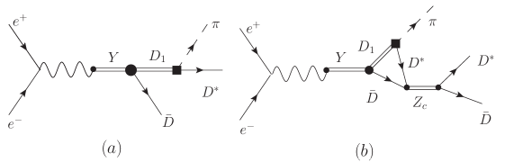
Figure 1: Feynman diagrams for the $e^{+}e^{-}\to Y(4260)\to D\bar{D}^{*}\pi$ via (a) the tree diagram and (b) an intermediate $Z_{c}$.

The coupling of $Y(4260)$ to $D_{1}\bar{D}$ in an $S$-wave are described by the Lagrangian Wang:2013cya ; Guo:2013zbw

$$\mathcal{L}_{Y} = \frac{y}{\sqrt{2}}Y^{i}\left(\bar{D}_{a}^{\dagger}D_{1a}^{i{\dagger}}-\bar{D}_{1a}^{i{\dagger}}D_{a}^{\dagger}\right)+{\rm H.c.},$$

where the (renormalized) effective coupling constant $y$ is in principle related to the probabilities of finding the components inside the $Y(4260)$ Weinberg:1963 ; Baru:2003 ; Guo:2013zbw , although for the large binding energy of the $Y(4260)$ a quantitative extraction of this quantity is hindered by the uncertainties of the method. We will also take into account the $Z_{c}(3900)$ contribution the same way as Ref. Wang:2013cya with $I^{G}(J^{PC})=1^{+}(1^{+-})$. The $S$-wave coupling of the $Z_{c}$ to the $D\bar{D}^{*}$ is described by a Lagrangian similar to Eq. (II) Wu:2013onz ,

$$\mathcal{L}_{Z}=z(\bar{D}_{b}^{*{\dagger}i}Z_{ba}^{i}D_{a}^{{\dagger}}-\bar{D}_{b}^{{\dagger}}Z_{ba}^{i}D_{a}^{*{\dagger}i})+h.c.$$ (1)

with the isotriplet

$$Z_{ba}=\left(\begin{array}[]{cc}\frac{1}{\sqrt{2}}Z^{0}&Z^{+}\\ Z^{-}&-\frac{1}{\sqrt{2}}Z^{0}\end{array}\right)_{ba}\ ,$$ (2)

A discussion of the bottom analogue can be found in Refs. Cleven:2013sq ; mehen . So far, we can only obtain information of this coupling constant from an analysis of the $Y(4260)\to J/\psi\pi\pi$ as performed in Ref. Wang:2013cya . With $|z|\approx 0.77~{}\mathrm{GeV}^{-1/2}$, the branching ratio $\mathcal{B}(Z_{c}\to D\bar{D}^{*})$ of about $20\%$ is compatible with the data.

The Lagrangian describing the interaction among the $\frac{3}{2}^{+}$ and $\frac{1}{2}^{-}$ spin multiplets and pions reads Colangelo:2005gb

$$\mathcal{L}_{D_{1}} = i\frac{h^{\prime}}{f_{\pi}}\big{[}3D_{1a}^{i}(\partial^{i}\partial^{j}\phi_{ab})D^{*j{\dagger}}_{b}-D_{1a}^{i}(\partial^{j}\partial^{j}\phi_{ab})D_{b}^{*i{\dagger}}+...\big{]}+{\rm H.c.},$$

where the coupling constant $|h^{\prime}|=(0.62\pm 0.08)~{}\mathrm{GeV}^{-1}$ is determined by the decay width $\Gamma_{D_{1}^{+}}=(25\pm 6)~{}\mathrm{MeV}$ Beringer:1900zz . The dots indicate terms not in the focus of this work.

For the $Z_{c}(3900)$ we use the following propagator Cleven:2011gp

$$G_{Z}(E)=\frac{1}{2}\frac{i}{E-m_{Z}-\Sigma_{DD^{*}}(E)+i\,\tilde{\Gamma}_{Z}/2}$$ (3)

with

$$\Sigma_{DD^{*}}(E)=z^{2}\frac{\mu_{DD^{*}}^{3/2}}{8\pi}\left[\sqrt{-2\epsilon}\,\theta(-\epsilon)-\sqrt{2\epsilon}\,\theta(\epsilon)\right],$$

where $\epsilon=E-m_{D}-m_{D^{*}}$ and the constant $\tilde{\Gamma}_{Z}$ accounts for the width from decay channels other than the $D\bar{D}^{*}$ such that the sum of Im$(2\Sigma_{Z}(E))$ evaluated at the pole and $\tilde{\Gamma}_{Z}$ gives the total width of the $Z_{c}$

In the $D_{1}\bar{D}$ molecular scenario, the propagator of $Y(4260)$ can be calculated analogous to Eq. (3) with $\Sigma_{DD^{*}}(E)$ replaced by

$$\hat{\Sigma}_{Y}\left(E\right) = \Sigma_{D_{1}D}\left(E\right)-\mathrm{Re}\big{[}\Sigma_{D_{1}D}\left(M_{Y}\right)+\left(E-M_{Y}\right)\partial_{E}\Sigma_{D_{1}D}(E)|_{E=M_{Y}}\big{]}.$$ (4)

Here we also have two parameters, i.e. one mass $M_{Y}$ and one constant residual width $\tilde{\Gamma}_{Y}$.

III Results

III.1 Line shapes of the $Y(4260)$ in the $J/\psi\pi\pi$ and $h_{c}\pi\pi$ channels

In this section, we present the fit results for line shapes of $e^{+}e^{-}\to Y(4260)\to J/\psi\pi\pi$ and $h_{c}\pi\pi$ in Fig. 2. The formalism used here is a straightforward extension of Ref. Wang:2013cya , i.e. including both box diagrams and $Z_{c}(3900)$ pole contributions simultaneously. It turns out that we need $S$-wave and $P$-wave background terms for the $J/\psi\pi\pi$ and $h_{c}\pi\pi$ channel, respectively, in order to fit the experimental data in the energy range of $[4.16,4.50]$ GeV for both processes. Since the partial waves of the $\pi\pi$ are $S$-wave for the background and mostly $D$-wave for the box diagrams and the $Z_{c}(3900)$ pole (since the $D_{1}$ decays to $D\pi$ in a $D$–wave, $cf$. Eq. (II)), there is no interference between them after the angular integration. Fit parameters are the mass of the $Y(4260)$, the non-$(D_{1}\bar{D}\to D^{*}\bar{D}\pi)$ width $\tilde{\Gamma}_{Y}$, a normalization constant and a factor for the strength of the background in each channel. The combined fit gives a reduced chi-square of 2 which seems sufficient given the simplified model used. As can be seen from Fig. 2 in both channels the proximity of the $D_{1}\bar{D}$ threshold in combination with a sizeable $D_{1}\bar{D}Y(4260)$ coupling constant $y$, which is the signature for a dominant molecular component of $Y(4260)$, leads to an asymmetric line shape. Due to this asymmetry especially in the $J/\psi\pi\pi$ channel, where the data are significantly better, the fit now gives a mass for the $Y(4260)$ significantly smaller than previous analyses, namely

$$M_{Y}(4260)=(4217.2\pm 2.0)~{}\mbox{MeV}$$ (5)

with the value of $\tilde{\Gamma}_{Y}=(55.91\pm 2.61)$ MeV, we see that the branching ratio for $Y(4260)\to D\bar{D}^{*}\pi$ via the intermediate $D\bar{D}_{1}$ is dominant within our model and can be as large as $60\%$. This finding is an important consistency check of our approach. Figure 2(a) and (b) show that the contribution of the $Z_{c}(3900)$ pole (short-dashed lines) is much smaller than that of the box diagrams (long-dashed lines) which is consistent with the results of Ref. Wang:2013cya .

One might question if it is sensible that the data in the $h_{c}\pi\pi$ channel above $4.35$ GeV is dominated by the background contribution. We therefore performed a series of additional fits including the higher thresholds ($D_{2}\bar{D}^{*}$, $D_{1}\bar{D}^{*}$) as well as the $Y(4360)$, as proposed in Refs. Aubert:2006ge ; Li:2013ssa . As expected these fits allowed us to remove the background contributions, however, the current data did not allow us to constrain sufficiently the values of the parameters. Especially with the current data it was not possible to decide whether a second resonance is needed. What is very important to this work is that regardless what dynamical content was used to fit the higher energies, the parameters of the $Y(4260)$ stayed largely unchanged. Due to this consideration we restrict ourselves only to a detailed discussion on the simplest fit in the rest of this work. .

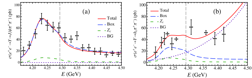
Figure 2: The cross sections for the $e^{+}e^{-}\to J/\psi\pi^{+}\pi^{-}$ and $e^{+}e^{-}\to h_{c}\pi^{+}\pi^{-}$ around the $Y(4260)$ mass region. The long-dashed, short-dashed, dotted and solid lines are the contributions from the $D_{1}\bar{D}$ box diagrams, the $Z_{c}(3900)$ pole, the $S$-wave background and the sum of them, respectively. The data in (a) are from Belle Yuan:2007sj and those in (b) from BESIII Ablikim:2013wzq , respectively.

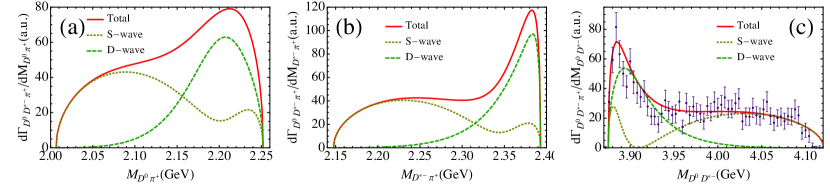
Figure 3: The $D^{0}\pi^{+}$, $D^{*-}\pi^{+}$ and $D^{0}D^{*-}$ invariant mass distributions for $Y(4260)\to D^{0}D^{*-}\pi^{+}$. The brown dotted, green dashed and red solid lines are the contributions from the $S$-wave, the $D$-wave and the sum of them, respectively.

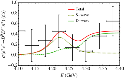
Figure 4: Predictions for the cross section of $e^{+}e^{-}\to D\bar{D}^{*}\pi$ with the dashed, dotted and solid lines denoting the contributions from $D$-wave, $S$-wave and the sum of them, respectively. Here the $D$-wave contribution is from our model due to the $D$-wave behaviour between $\bar{D}^{*}$ and $\pi$. Meanwhile the $S$-wave contribution means the background contribution with the $\bar{D}^{*}$ and $\pi$ in $S$-wave. The data are from Belle Pakhlova:2009jv .

III.2 Line shapes of the $Y(4260)$ in the $D\bar{D}^{*}\pi$-channel and the invariant mass distributions

As discussed in Sec. I, there are two kinds of diagrams contributing to $D\bar{D}^{*}\pi$ channels, i.e. tree diagram (Fig. 1 (a)) and the $Z_{c}(3900)$ resonant contribution (Fig. 1 (b)). Since $D_{1}$ decays to $D^{*}\pi$ is in $D$-wave, the contribution from the $D_{1}$ pole results in an enhancement of the $D^{*}\pi$ spectrum at the higher mass end, i.e. approaching the $D_{1}$ pole at 2.42 GeV — $cf$. the green dashed line in Fig. 3 (b). Furthermore, due to the same reason, the lower ends of both the $D\pi$ and $D^{*}\pi$ invariant mass distributions are strongly suppressed — $cf$. the green dashed lines in Fig. 3 (a) and (b).

A significant fraction of the enhancement near the $D\bar{D}^{*}$ threshold, as shown by the green dashed line in Fig. 3 (c), may be understood as a reflection of the enhancement predicted in $\bar{D}^{*}\pi$. With the current data quality and the level of sophistication of our model we are not able to disentangle this from the contribution of $Z_{c}(3900)$. The apparent discrepancy between our model prediction and the BESIII data Ablikim:2013xfr should come from some $\bar{D}^{*}\pi$ $S$-wave contribution that we here include as an additional, small contribution to the $Y(4260)$ wave function. To investigate this idea further we include this additional $S$–wave. Now the full amplitude can be expressed as

$$\mathcal{M}_{D\bar{D}^{*}\pi} = \epsilon_{Y}^{a}\epsilon_{\bar{D}^{*}}^{b}\left[C_{S}\delta^{ab}+C_{D}(E,M_{D\bar{D}^{*}},M_{\bar{D}^{*}\pi})\left(\hat{q}^{a}\hat{q}^{b}-\frac{1}{3}\delta^{ab}\right)\right]$$ (6)

with $C_{S}$ the $S$-wave strength and $C_{D}(E,M_{D\bar{D}^{*}},M_{\bar{D}^{*}\pi})$ the $D$-wave strength. The $S$-wave strength can be parameterized as

$$C_{S}=\alpha(M_{D\bar{D}^{*}}^{2}+\beta)G_{Z}(E)$$ (7)

which respects Watson theorem as long as $\alpha$ and $\beta$ are real numbers . The $D$-wave strength is extracted from our model, i.e. the sum of Fig. 1 (a) and (b).

From the fit to the $D^{0}D^{*-}$ spectrum from $3.88~{}\mathrm{GeV}$ to $4.1~{}\mathrm{GeV}$, $cf$. Fig. 3 (c), we obtain $|\alpha|=(6.72\pm 0.17)~{}\mathrm{GeV}^{-1}$, $\beta=(-15.28\pm 0.01)~{}\mathrm{GeV}^{2}$ and $\chi^{2}/d.o.f.=59.02/(57-3)$. Since in the invariant mass spectrum there is no interference between the $S$– and the $D$–wave contribution, the fit does not allow one to fix the sign of $\alpha$. In what follows we chose $\alpha<0$ in order to get the correct angular distributions as discussed in the next section. The result of the fit as well as the impact of the $S$–wave on the other invariant mass spectra is shown as the red solid line in the three panels of Fig. 3. The individual contribution from the $S$-wave is displayed by the brown dotted line. As one can see, although the small admixture of additional $S$-wave component in the $Y(4260)$ wave function will make the suppression of the lower end of the $D\pi$ and $D^{*}\pi$ invariant mass distribution not as significant as before, in the region that matters the most for both the $Y(4260)$ and the $Z_{c}(3900)$ the $D$–wave contribution still dominates, i.e. the $D_{1}\bar{D}$–component is still the most important part of the $Y(4260)$ wave function.

With all the parameters from the fits above, i.e. the line shapes of $Y(4260)$ in $e^{+}e^{-}\to Y(4260)\to J/\psi\pi\pi$ and $h_{c}\pi\pi$ processes and the invariant mass distributions in $e^{+}e^{-}\to Y(4260)\to D\bar{D}^{*}\pi$ process, measured close to the pole of the $Y(4260)$, one can predict also the line shape for $D\bar{D}^{*}\pi$ process. The green dashed line in Fig. 4 shows this prediction when only the $D_{1}\bar{D}$ component is included. Again, a nontrivial structure arises from the presence of the $S$-wave $D_{1}\bar{D}$ threshold. Especially, the rate predicted above the nominal $D_{1}\bar{D}$ threshold is higher than at the actual $Y(4260)$ peak position. Although this picture is changed quantitatively by the inclusion of the additional $S$–wave, the basic features remain. Especially, if the $Y(4260)$ is a hadronic molecule, one will not find a Breit-Wigner line shape around 4.26 GeV in $e^{+}e^{-}\to Y(4260)\to D\bar{D}^{*}\pi$. Our prediction is consistent with the existing data  Pakhlova:2009jv , although improved measurements are clearly needed to confirm or disprove our predictions.

III.3 Angular distributions in the $D\bar{D}^{*}\pi$ channel

Figure 5: Angular distribution of the pion in the rest frame of the $Y(4260)$ with respect to the beam axis (Jackson angle). The legends are the same as that in Fig. 3. The experimental data are from Ref. Ablikim:2013xfr .

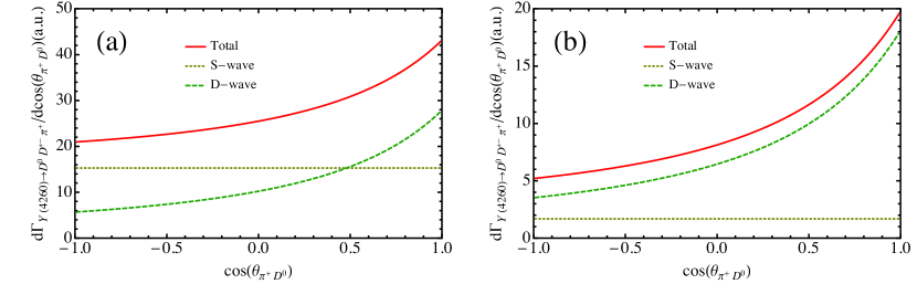
Figure 6: The partial width of $Y(4260)\to D^{0}D^{*-}\pi^{+}$ is shown in terms of the relative angle between the $\pi^{+}$ and the $D^{0}$ in the $D^{0}D^{*-}$ rest frame. The legends are the same as that in Fig. 3. Left panel: using the whole Dalitz plot; right panel: with a cut on small $D\bar{D}^{*}$ invariant masses imposed, i.e. using the events from the $D\bar{D}^{*}$ threshold to $3.92~{}\mathrm{GeV}$.

With the parameters fixed by the fit to the $D\bar{D}^{*}$ invariant mass distribution in the previous section, we now investigate two angular distributions: the Jackson angle of the spectator pion, $\theta_{\pi}$, and the $D$-$\pi$ helicity angle, $\theta_{\pi D}$.

The angular distribution of the Jackson angle of the spectator pion, $\theta_{\pi}$, defined as the angle between pion and the beam direction in the overall center-of-mass frame Ablikim:2013xfr , is shown in Fig. 5. Since the experimental data are taken around the $Z_{c}(3900)$ pole, we integrate the $D\bar{D}^{*}$ invariant mass from the threshold to $3.92~{}\mathrm{GeV}$, $cf$. Fig. 3 (c). As shown in Fig. 5, the large $D$-wave interfering with the strength of the small $S$-wave fixed before and having chosen the sign of $\alpha$ such that there is a destructive interference between $S$– and $D$–waves, leads to an almost-flat angular distribution (a more general discussion about the angular distribution of the spectator pion can be found in App. A). Note, the information encoded in the Jackson angle goes beyond that contained in the Daliz plot. Thus, the agreement we find between our calculation and the data for $\theta_{\pi}$ is non-trivial, although we fit to the $D\bar{D}^{*}$–invariant mass distribution.

The helicity angle $\theta_{\pi D}$ is defined as the relative angle between $\pi$ and $D$ in $D\bar{D}^{*}$ rest frame. Our results for this observable are shown as the green dashed, brown dotted and red solid lines for the $D$–wave from the molecular component of the $Y(4260)$, the additional $S$–wave and the sum of both are shown in Fig. 6. In the left panel the whole range of invariant masses allowed kinematically is integrated. As one can see, the $D$–wave coming the molecular component of the $Y(4260)$ leads to a clearly visible forward–backward asymmetry that stays prominent also after inclusion of the additional $S$ wave. This signal can be further enhanced by imposing a cut on small $D\bar{D}^{*}$ invariant masses, i.e. from the $D\bar{D}^{*}$ threshold to $3.92~{}\mathrm{GeV}$, as shown in the right panel. Clearly this observable is very sensitive to the $D_{1}\bar{D}$ component of $Y(4260)$. So far an empirical value is available only for the ratio Ablikim:2013xfr

$$\mathcal{A}=\frac{n_{>0.5}-n_{<0.5}}{n_{>0.5}+n_{<0.5}}=(0.12\pm 0.06)$$ (8)

reflecting the asymmetry of events between $|\cos(\theta_{\pi D})|>0.5$ and $|\cos(\theta_{\pi D})|<0.5$, where the full range of invariant masses allowed kinematically was included. From integrating the observable shown in the left panel of Fig. 6 we find $\mathcal{A}=0.0,~{}0.11,~{}0.05$ for the $S$ wave, $D$ wave and the sum of both, respectively. We can see that a pure $D$-wave contribution with $\mathcal{A}=0.11$ agrees with the experimental data perfectly. Nevertheless the other two results deviate by less than two sigma. Given the distributions shown in Fig. 6, even with the present experimental accuracy, a more decisive observable might be the forward–backward asymmetry of $\theta_{\pi D}$

$$\mathcal{A}_{fb}=\frac{n_{>0}-n_{<0}}{n_{>0}+n_{<0}}\ .$$ (9)

From our calculation we find $\mathcal{A}_{fb}=0.0,0.37,0.16$ for S-wave, D-wave and the sum of them, when the whole kinematic region is integrated.

To unambiguously determine how large the $S$-wave contribution is improved data is needed. In addition, we need to do an overall fit to all the available data in $J/\psi\pi\pi$, $h_{c}\pi\pi$, $D\bar{D}^{*}\pi$ and $D^{*}\bar{D}^{*}\pi$ processes which is beyond the purpose of this work.

IV summary

In summary, we have demonstrated in this study that, if the $Y(4260)$ is a $D_{1}\bar{D}$ molecule, quite unusual line shapes should emerge naturally in both the $J/\psi\pi\pi$ and $h_{c}\pi\pi$ channels. As a consequence the fits return a pole location of the $Y(4260)$ significantly lower than that found in earlier studies. In addition, the $D\bar{D}^{*}\pi$ channel is predicted to be the dominant decay mode of the $Y(4260)$. We find that, since the $D_{1}\bar{D}$ threshold is only a few tens of MeV above the location of the $Y(4260)$, the $D\bar{D}^{*}\pi$ rate gets strongly enhanced above the nominal $D_{1}\bar{D}$ threshold. A detailed study of the $D\bar{D}^{*}$ invariant mass distribution revealed that in addition to the dominant $D_{1}\bar{D}$–component of the $Y(4260)$ that leads to $D$–wave pions in the $D\bar{D}^{*}\pi$ channel, a subleading contribution that produces $S$–wave pions is needed. It is important to stress that once this additional term is fixed from the invariant mass distribution its interference with the dominant $D$–wave term at the same time gives a flat angular distribution for $\theta_{\pi}$ — the Jacobi angle of the pion — consistent with the data. Fortunately there is another angular distribution, where the $D$–wave still leads to a visible imprint, namely, the $\pi D$-helicity angle. Even when the $S$ wave is added, there is still a visible forward–backward asymmetry in the prediction, which can be enhanced further by introducing a cut in the $D\bar{D}^{*}$ invariant mass ($cf$. Fig. 6). Thus, a coherent analysis of all decay channels of the $Y(4260)$ with improved data will allow one to test, if this state indeed shows a (predominant) $D_{1}\bar{D}$–molecular structure.

Appendix A General discussion of the $\cos\theta_{\pi}$ distribution

In this appendix a general discussions is presented for the distribution of the pion angle $\theta_{\pi}$, defined relative to the beam direction in the $e^{+}e^{-}$ rest frame for the process $e^{+}e^{-}\to Y(4260)\to Z_{c}(3900)\pi$. For the general amplitude of $Y(4260)\to Z_{c}(3900)\pi$ we write

$$\mathcal{M} = \epsilon_{Y}^{a}\epsilon_{Z_{c}}^{b}\left(C_{S}\delta^{ab}+C_{D}\left(\hat{q}^{a}\hat{q}^{b}-\frac{1}{3}\delta^{ab}\right)\right)\ .$$ (10)

The parameters $C_{S}$ for the $S$-wave strength and $C_{D}$ for the $D$-wave strength contain all information on the dynamics. One finds

$$\sum_{\text{polarizations}}|\mathcal{M}|^{2}=2C_{S}^{2}-2C_{S}C_{D}\cos^{2}\theta_{\pi}+\frac{2C_{S}C_{D}}{3}-\frac{C_{D}^{2}\cos^{2}\theta_{\pi}}{3}+\frac{5C_{D}^{2}}{9}$$ (11)

where the sum of the polarizations

$$\sum_{\lambda=1,2}\epsilon_{Y}^{\lambda a}\epsilon_{Y}^{*\lambda b} = \delta^{ab}-\delta^{a3}\delta^{b3},~{}\quad\sum_{\lambda=1,2,3}\epsilon_{Z_{c}}^{\lambda a}\epsilon_{Z_{c}}^{*\lambda b}=\delta^{ab}\$$ (12)

were used with the third component pointing to the beam direction. The first expression contains the fact that in $e^{+}e^{-}$ collisions the photon and correspondingly the $Y(4260)$ are produced transversely. From Eq. (11) one obtains a flat angular distribution not only when $C_{D}=0$, corresponding to a pure $S$–wave, but also for $C_{D}=-6C_{S}$, where the $D$–wave dominates.

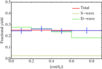
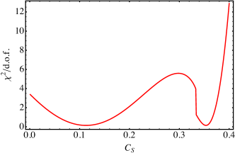
Figure 7: Left panel: Pion angular distribution from the general amplitude of Eq. (10). The green dashed, brown dotted and red solid lines are the contributions from $D$-wave, $S$-wave and the sum of them. The experimental data are from Ref. Ablikim:2013xfr . Right panel: $\chi^{2}$ in terms of the $S$-wave strength parameter $C_{S}$ — for each value of $C_{S}$ the parameter $C_{D}$ is refitted.

To be specific, we apply this general parameterization to the data for the pion angular distribution given in Ref. Ablikim:2013xfr . A fit for the parameters $C_{S}$ and $C_{D}$ gives two solutions, $cf$. Table 1, in agreement with the discussion above. The individual contributions for the best fit with $D$–wave dominance are shown in the left panel of Fig. 7. In the right panel of this figure we show the variation of the $\chi^{2}$–value, when for a fixed value of $C_{S}$ the parameter $C_{D}$ is fitted to the data. As one can see the $\chi^{2}$–minimum referring to the $D$–wave dominance is rather flat — this means that no fine tuning in the relative strength of the amplitudes is necessary to get a flat angular distribution in $\theta_{\pi}$; all it takes is an admixture of a small, non–vanishing $S$–wave amplitude.

Table 1: The parameters $C_{S}$ and $C_{D}$ of the two solutions, i.e. the $S$-wave dominant and the $D$-wave dominant schemes, are listed in this table.

parameters	$S$-wave dominant	$D$-wave dominant
$C_{S}$	$0.35\pm 0.01$	$0.11\pm 0.02$
$C_{D}$	$0.01\pm 0.04$	$-0.71\pm 0.01$
$\chi^{2}/d.o.f.$	0.23	0.23

References

- (1) B. Aubert et al. [BaBar Collaboration], Phys. Rev. Lett. 95, 142001 (2005).
- (2) N. Brambilla et al., Eur. Phys. J. C 71, 1534 (2011).
- (3) M. Ablikim et al. [BESIII Collaboration], Phys. Rev. Lett. 110, 252001 (2013).
- (4) Z. Q. Liu et al. [Belle Collaboration], Phys. Rev. Lett. 110, 252002 (2013).
- (5) T. Xiao, S. Dobbs, A. Tomaradze and K. K. Seth, Phys. Lett. B 727, 366 (2013) [arXiv:1304.3036 [hep-ex]].
- (6) M. Ablikim et al. [BESIII Collaboration], arXiv:1308.2760 [hep-ex].
- (7) M. Ablikim et al. [BESIII Collaboration], Phys. Rev. Lett. 111, 242001 (2013) [arXiv:1309.1896 [hep-ex]].
- (8) Q. Wang, C. Hanhart and Q. Zhao, Phys. Rev. Lett. 111, 132003 (2013).
- (9) S.-L. Zhu, Phys. Lett. B 625, 212 (2005).
- (10) E. Kou and O. Pene, Phys. Lett. B 631, 164 (2005).
- (11) F. E. Close and P. R. Page, Phys. Lett. B 628, 215 (2005).
- (12) M. B. Voloshin, Prog. Part. Nucl. Phys. 61, 455 (2008).
- (13) S. Dubynskiy and M. B. Voloshin, Phys. Lett. B 666, 344 (2008).
- (14) X. Li and M. B. Voloshin, arXiv:1309.1681 [hep-ph].
- (15) G.-J. Ding, Phys. Rev. D 79, 014001 (2009).
- (16) M.-T. Li, W.-L. Wang, Y.-B. Dong and Z.-Y. Zhang, arXiv:1303.4140 [nucl-th].
- (17) L. Y. Dai, M. Shi, G.-Y. Tang and H. Q. Zheng, arXiv:1206.6911 [hep-ph].
- (18) F. J. Llanes-Estrada, Phys. Rev. D 72, 031503 (2005).
- (19) A. Martinez Torres et al., Phys. Rev. D 80, 094012 (2009) [arXiv:0906.5333 [nucl-th]].
- (20) J. Beringer et al. [Particle Data Group Collaboration], Phys. Rev. D 86, 010001 (2012).
- (21) X. Li and M. B. Voloshin, Phys. Rev. D 88, 034012 (2013).
- (22) Q. Wang et al., Phys. Rev. D 89, 034001 (2014) [arXiv:1309.4303 [hep-ph]].
- (23) F.-K. Guo et al., Phys. Rev. D 88, 054007 (2013).
- (24) F.-K. Guo et al., Phys. Lett. B 725, 127 (2013).
- (25) C.-Z. Yuan, arXiv:1310.0280 [hep-ex].
- (26) F.-K. Guo, C. Hanhart and U.-G. Meißner, Phys. Rev. Lett. 103, 082003 (2009) [Erratum-ibid. 104, 109901 (2010)].
- (27) F.-K. Guo et al., Phys. Rev. D 83, 034013 (2011).
- (28) S. Weinberg, Phys. Rev. 130 (1963) 776.
- (29) V. Baru , Phys. Lett. B 586 (2004) 53 [hep-ph/0308129].
- (30) X. -G. Wu, C. Hanhart, Q. Wang and Q. Zhao, Phys. Rev. D 89, 054038 (2014) [arXiv:1312.5621 [hep-ph]].
- (31) T. Mehen and J. Powell, Phys. Rev. D 88 (2013) 3, 034017 [arXiv:1306.5459 [hep-ph]].
- (32) M. Cleven et al., Phys. Rev. D 87, 074006 (2013).
- (33) P. Colangelo, F. De Fazio and R. Ferrandes, Phys. Lett. B 634, 235 (2006).
- (34) M. Cleven, F.-K. Guo, C. Hanhart and U.-G. Meißner, Eur. Phys. J. A 47, 120 (2011).
- (35) C. Z. Yuan et al. [Belle Collaboration], Phys. Rev. Lett. 99, 182004 (2007).
- (36) B. Aubert et al. [BaBar Collaboration], Phys. Rev. Lett. 98, 212001 (2007).
- (37) C. Hanhart, Phys. Lett. B 715 (2012) 170 [arXiv:1203.6839 [hep-ph]].
- (38) M. Ablikim et al. [BESIII Collaboration], Phys. Rev. Lett. 112, 022001 (2014) [arXiv:1310.1163 [hep-ex]].
- (39) G. Pakhlova et al. [Belle Collaboration], Phys. Rev. D 80, 091101 (2009).