Fast updating algorithms for latent semantic indexing

Abstract

This paper discusses a few algorithms for updating the approximate Singular Value Decomposition (SVD) in the context of information retrieval by Latent Semantic Indexing (LSI) methods. A unifying framework is considered which is based on Rayleigh-Ritz projection methods. First, a Rayleigh-Ritz approach for the SVD is discussed and it is then used to interpret the Zha–Simon algorithms [SIAM J. Scient. Comput. vol. 21 (1999), pp. 782-791]. This viewpoint leads to a few alternatives whose goal is to reduce computational cost and storage requirement by projection techniques that utilize subspaces of much smaller dimension. Numerical experiments show that the proposed algorithms yield accuracies comparable to those obtained from standard ones at a much lower computational cost.

1 Introduction

Latent Semantic Indexing (LSI), introduced in [9], is a well-established text mining technique that aims at finding documents in a given collection that are relevant to a user’s query. The method is a variation of the Principal Component Analysis (PCA) [5], where the multidimensional text dataset is projected to a low-dimensional subspace. When properly defined, this subspace captures the essence of the original data. In the projected space, semantically similar documents tend to be close to each other in a certain measure, which allows to compare them according to their latent semantics rather than a straightforward word matching.

LSI can be viewed as an extension of the vector space model for Information Retrieval (IR) [23]. As such, it begins with a preprocessing phase (see, e.g, [1, 28]) to summarize the whole text collection in the $m$-by-$n$ term-document matrix $A$, where $m$ and $n$ are the total numbers of terms and documents in the collection, respectively. Thus, each column of $A$ represents a separate document, where nonzero entries are the weights, or essentially the frequencies, of the terms occurring in this document. For the discussion of the available term weighting schemes we refer the reader to [17].

We consider a widely used and standard implementation of LSI that is based on the partial Singular Value Decomposition (SVD) [12] of the term-document matrix. In this case, LSI resorts to calculating the singular triplets $(\sigma_{j},u_{j},v_{j})$ associated with the $k$ largest singular values $\sigma_{1}\geq\sigma_{2}\geq\ldots\geq\sigma_{k}\geq 0$ of $A$. Throughout, we call these $k$ triplets the dominant singular triplets. The left singular vectors $u_{j}$ are then used to construct the low-dimensional subspace for data projection and, along with $\sigma_{j}$ and the right singular vectors $v_{j}$, to evaluate the relevance scores. We note that a number of “SVD avoiding” LSI algorithms have been proposed in recent years, e.g., [6, 8, 10, 16, 17], for example, by replacing the SVD by the Lanczos decomposition. We will briefly discuss one such alternative based on using Lanczos vectors.

Given a user’s query $q$, formalized by a vector of size $m$, i.e., regarded as a document, the associated vector $r$ of $n$ relevance scores is evaluated by

$$r=\mbox{diag}\left(\gamma_{1},\ldots,\gamma_{n}\right)\left(V_{k}\Sigma_{k}^{1-\alpha}\right)\Sigma_{k}^{\alpha}U_{k}^{T}q.$$ (1)

Here, $\Sigma_{k}=\mbox{diag}\left\{\sigma_{1},\sigma_{2},\ldots,\sigma_{k}\right\}\in\mathbb{R}^{k\times k}$; $U_{k}=[u_{1},\ldots,u_{k}]\in\mathbb{R}^{m\times k}$ and $V_{k}=[v_{1},\ldots,v_{k}]\in\mathbb{R}^{n\times k}$ are the matrices of the orthonormal left and right singular vectors, respectively. The diagonal elements $\gamma_{j}$ are chosen to normalize the rows of $V_{k}\Sigma_{k}^{1-\alpha}$ so that each row has a unit norm. The scalar $\alpha$ is a splitting parameter and has no affect on ranking if the normalization is disabled ($\gamma_{j}=1$); see, e.g., [17] for a detailed discussion.

The $j$-th entry of $r$, denoted by $r(j)$, quantifies the relevance between the $j$-th document and the query. The documents with the highest relevance scores are returned to the user in response to the query $q$. Note that, for example, in the case where $\alpha=0$, $r(j)$ is the (scaled) cosine of the angle between the $j$-th projected document $U_{k}^{T}a_{j}$ and the projected query $U_{k}^{T}q$.

In practical applications, where the amount of data tends to be extremely large, the implementation of LSI faces two major difficulties. The first difficulty is the requirement to compute the dominant singular triplets of a very large matrix, a problem that has been relatively well investigated. Possible solutions include invoking iterative singular value solvers, e.g., [4, 14], that take advantage of sparsity and fast matrix-vector products. Other solutions leverage specific spectral properties of the term-document matrices, and rely on incremental or divide-and-conquer techniques; e.g., [29, 7].

The second computational difficulty of LSI is related to the fact that document collections are dynamic, i.e., the term-document matrices are subject to repeated updates. Such updates result from adding, e.g., new documents or terms to the collection. In the language of the vector space model, this translates into adding new columns or rows to $A$. Another type of update is when the term weights are corrected, which corresponds to modifying entries of the term-document matrix. Thus, in order to maintain the quality of the subsequent query processing, the available singular triplets should be accordingly modified after each update. A straightforward solution to this problem is to recompute the partial SVD of the updated term-document matrix from scratch. However, even with the most sophisticated singular value solvers, this naive approach is not practical as it is exceedingly costly for realistic large-scale text collections. Therefore, a critical question is how to update the available $\Sigma_{k}$, $U_{k}$, and $V_{k}$ without fully recomputing the high-cost partial SVD of the modified matrix, so that the retrieval quality is not affected.

This paper addresses this specific question. It starts by revisiting the well-known updating algorithms of Zha and Simon [29], currently the state-of-the-art approach for the LSI updating problem. Specifically, the paper interprets these schemes as Rayleigh-Ritz projection procedures. A by-product of this viewpoint is a min-max type characterization of the Ritz singular values obtained in the process. On the practical side, this projection viewpoint unravels a certain redundancy in the computations, showing that it is possible to further improve the efficiency of the techniques without sacrificing retrieval quality. Based on these findings, we propose a family of new updating algorithms which can be substantially faster and less storage-demanding than the methods in [29].

The motivation for the present work comes from the observation that the methods in [29] (reviewed in more detail in Section 3) rely on the SVD of a $(k+p)$-by-$(k+p)$ dense matrix and orthogonalization of $p$ ($m$- or $n$-dimensional) vectors, where $p$ denotes the size of the update, i.e., the number of added columns, rows, or corrected terms. In particular, this suggests that the computational complexity of the overall updating procedure scales cubically with respect to $p$.

While the effect of the cubic scaling is marginal for smaller document collections, where the update sizes are typically given by only a few terms or documents, the situation becomes different for large-scale datasets. In this case, even if $p$ is a tiny fraction of terms or documents, its (cubed) value may be large enough to noticeably affect the efficiency of the updating methods. In other words, for $p$ sufficiently large, the computational costs associated with the SVD of a $(k+p)$-by-$(k+p)$ matrix and orthogonalization (QR decomposition) of $p$ vectors become non-negligible and may dominate the overall updating procedure.

Another context in which larger updates are to be processed can be found in the recent works [25, 18], where the authors suggest to postpone invoking the updating schemes from [29] until the update size becomes sufficiently large. In between the updates, a fast folding-in procedure [3, 2] is performed, which can be viewed as a form of PCA out-of-sample embedding [26] applied in the context of LSI. Such a combination of folding-in and updates, called folding-up, has been shown to yield a substantial reduction in the time spent for updating without a significant loss in the retrieval accuracy.

To adapt their algorithms to the cases of large $p$, the authors of [29] suggest splitting the current update into a series of smaller sequential updates, and performing the whole updating procedure in an incremental fashion. While this approach indeed leads to memory savings, it requires more time to complete the overall updating task than to perform the whole update at once. This can be seen, e.g., from Table $4.2$ in the original paper [29], after multiplying the reported average CPU times per update by the number of updates. A similar observation has been made in [25, Table 1]. Additionally, as has also been observed in [25], breaking a given update into a sequence of smaller updates can potentially lead to a faster deterioration of the retrieval accuracy.

The updating algorithms proposed in this paper require orthonormalizing sets of significantly fewer vectors than those in [29] and rely on the SVD of much smaller matrices. As a result, the new schemes are less sensitive to the increase in the update sizes. As shown in our experiments, the presented algorithms significantly reduce the runtime, whereas the retrieval accuracy is not affected.

Finally, let us recall that the methods in [29] were introduced as a solution to the problem of the deteriorating retrieval accuracy exhibited by existing methods [3, 19] in the mid-1990s. This solution essentially traded the SVD of a $k$-by-$k$ matrix in [3, 19] for the above mentioned orthonormalization of a set of $p$ extra vectors plus a $(k+p)$-by-$(k+p)$ SVD. The updating schemes introduced in this work can be viewed as a compromise between [3, 19] and [29], where the runtime resembles that of the former while the retrieval accuracy is comparable to the latter.

The rest of the paper is organized as follows. Projection methods for the SVD are reviewed in Section 2 followed by a discussion of their applications to LSI in Section 3. In Section 4 a number of alternative algorithms are presented with a goal of reducing cost. Section 5 presents numerical experiments to test the various methods introduced, and Section 6 concludes the paper with a few remarks.

2 Projection methods for singular value problems

It will be useful to explore projection methods for the singular value problem in order to understand the mechanisms at play when updating the SVD. We begin with a little background on standard projection methods. Recall that given a Hermitian $n\times n$ matrix $M$, a Rayleigh-Ritz (RR) projection method extracts approximate eigenpairs for $A$ from a search subspace $\mbox{{span}}\{Z\}$, where $Z\ \in\mathbb{R}^{n\times s}$. It does so by imposing two conditions. First, any approximate eigenvector must belong to $\mbox{{span}}\{Z\}$, i.e., it can be written as $z=Zc$ (where $c\ \in\mathbb{R}^{s}$). Second, the approximate eigenpair $(\theta,z)$ must satisfy the Galerkin condition that the residual is orthogonal to $\mbox{{span}}\{Z\}$, i.e., we must have $(M-\theta I)z\perp\mbox{{span}}\{Z\}$. This yields the projected $s\times s$ eigenvalue problem $(Z^{T}MZ)c=\theta c$ from which we obtain the Ritz values $\theta_{i}$, the corresponding eigenvectors $c_{i}$, and the Ritz vectors $z_{i}=Zc_{i},i=1,\ldots,s$. Details can be found in, e.g., [20, 21].

2.1 Application to the SVD

Consider now the singular value problem for a matrix $A\in\ \mathbb{R}^{m\times n}$. The above projection procedure can be adapted to the singular value problem in a number of ways. For example, we can apply the RR idea to one of the two standard eigenvalue problems with either $A^{T}A$ or $AA^{T}$. This, however, is not appealing due to its “non-symmetric” nature: it puts an emphasis on one set of singular vectors (left or right) and will encounter difficulties with the smallest singular values due to their squaring. An alternative approach is to apply the Rayleigh-Ritz procedure to the augmented matrix

$$B=\begin{pmatrix}0&A\\ A^{T}&0\end{pmatrix}.$$ (2)

We will consider this second approach as it leads more naturally to a separation of the right and left singular vectors. A straightforward application of the RR procedure would now use a subspace $\mbox{{span}}\{Z\}$ where $Z\in\ \mathbb{R}^{(m+n)\times s}$ and would write a test eigenvector in the form $z=Zc$ where $c\ \in\mathbb{R}^{s}$. It then imposes the Galerkin condition $Z^{T}(B-\theta I)Zc=0$ from which Ritz values and vectors are obtained. Observe that $z$ can be written as $z=\left(u\atop v\right)$, where $u\ \in\mathbb{R}^{m}$ approximates a left singular vector of $A$ and $v\ \in\mathbb{R}^{n}$ approximates a right singular vector of $A$.

One weakness of this viewpoint is that there is no reason why the left approximate singular vector (vector $u$, i.e, top part of $z=Zc$) and the right approximate singular vector (vector $v$ or bottom part of $z=Zc$) should be expressed in the basis $Z$ with the same basis coefficients $c$. In practice, we have two bases available, one for the left singular vectors and one for the right singular vectors. Therefore, let $U\ \in\mathbb{R}^{m\times s_{1}}$ be a basis for the left search subspace and $V\ \in\mathbb{R}^{n\times s_{2}}$ a basis for the right search subspace, with $s_{1}+s_{2}=s$. Both $U$ and $V$ are assumed to be orthonormal bases and note that $s_{1}$ and $s_{2}$ need not be the same. Then, the approximate right singular vector can be expressed as $u=Uf$ (with $f\ \in\mathbb{R}^{s_{1}}$) and the approximate left singular vector as $v=Vg$ (with $g\ \in\mathbb{R}^{s_{2}}$). This gives us $s_{1}+s_{2}=s$ degrees of freedom. To extract $f$ and $g$ we would need $s$ constraints which are to be imposed on the residual vector $(B-\theta I)z$ where $z=\left(u\atop v\right)$. This residual is

$$r=\begin{pmatrix}Av-\theta u\\ A^{T}u-\theta v\end{pmatrix}.$$ (3)

It is natural to impose the condition that the first part, which is in $\mathbb{R}^{m}$, be orthogonal to $\mbox{{span}}\{U\}$ and the second part, which is in $\mathbb{R}^{n}$, be orthogonal to $\mbox{{span}}\{V\}$ :

$$\left\{\begin{array}[]{ccc}U^{T}(AVg-\theta Uf)&=&0\\ V^{T}(A^{T}Uf-\theta Vg)&=&0\end{array}\right..$$ (4)

System (4) leads to the projected singular value problem $Hg=\theta f$ and $H^{T}f=\theta g$, where $H=U^{T}AV$. Let $(\theta_{i},f_{i},g_{i})$ be the singular triplets of the projected matrix $H$, i.e., $Hg_{i}=\theta_{i}f_{i}$ and $H^{T}f_{i}=\theta_{i}g_{i}$; $i=1,\ldots,\min\{s_{1},s_{2}\}$. Then the scalars $\theta_{i}$ are the Ritz singular values, the vectors $Uf_{i}$ are the left Ritz singular vectors of $A$, and the vectors $Vg_{i}$ are the right Ritz singular vectors of $A$. It is important to note that when $\theta_{i}>0$ then the above conditions imply that $\|f_{i}\|=\|g_{i}\|$. This can be easily seen by multiplying (from left) both sides of the equality $Hg_{i}=\theta_{i}f_{i}$ by $f_{i}^{T}$ and of the equality $H^{T}f_{i}=\theta_{i}g_{i}$ by $g_{i}^{T}$.

The “doubled” form of the Galerkin condition (4) has been considered in [15] in the context of the correction equation for a Jacobi-Davidson approach. These are not quite standard Galerkin conditions since they amount to two separate orthogonality constraints. However, it is also possible to interpret this approach as a standard Galerkin/RR procedure, which is the viewpoint we develop next.

Consider the following new basis for a subspace of $\mathbb{R}^{m+n}$ given by

$$Z=\left[\begin{matrix}U&0\\ 0&V\end{matrix}\right].$$ (5)

Then a test vector $z$ in $\mbox{{span}}\{Z\}$ can be written as

$$z=\left[\begin{matrix}U&0\\ 0&V\end{matrix}\right]\begin{pmatrix}f\\ g\end{pmatrix}=\begin{pmatrix}u\\ v\end{pmatrix}.$$ (6)

Clearly, the residual vector $(B-\theta I)z$ of this test vector for the approximate eigenvalue $\theta$ and the matrix $B$ is again given by (3) and the standard Galerkin condition $Z^{T}r=0$ yields exactly the doubled form (4) of the Galerkin condition.

Proposition 1.

The RR procedure defined by the doubled form of the Galerkin condition (4) is mathematically equivalent to the standard RR procedure applied to the symmetric matrix $B$ using the basis given by (5).

In essence the procedure defined in this way puts an emphasis on not mixing the $U$-space and the $V$-space as indicated by zeros in the appropriate locations in (5) and this is achieved by a restricting the choice of basis for the search space. This is in contrast to the general procedure described at the very beginning of this section, where $Z$ makes no distinction between the $U$- and $V$- spaces.

2.2 Application to LSI

Let $A$ be a certain term-document matrix considered at some stage in the updating and querying process and let $U\in\mathbb{R}^{m\times s_{1}}$ and $V\in\mathbb{R}^{n\times s_{2}}$ be the orthonormal bases of the left and right search subspaces, respectively. Suppose that our goal is to construct approximations $(\tilde{\sigma}_{i},\tilde{u}_{i},\tilde{v}_{i})$ to the $k$ dominant singular triplets $(\sigma_{i},u_{i},v_{i})$, such that $\tilde{\sigma}_{i}=\theta_{i}\geq 0$, $\tilde{u}_{i}=Uf_{i}$, and $\tilde{v}_{i}=Vg_{i}$; $i=1,\ldots k$. The matrices of the singular values and vectors of $A$ are then approximated by

$$\tilde{\Sigma}_{k}=\Theta_{k},\quad\tilde{U}_{k}=UF_{k},\quad\tilde{V}_{k}=VG_{k}\;;$$ (7)

where $\Theta_{k}=\mbox{diag}\left\{\theta_{1},\ldots,\theta_{k}\right\}$, and $F_{k}=[f_{1},\ldots,f_{k}]\in\mathbb{R}^{s_{1}\times k}$ and $G_{k}=[g_{1},\ldots,g_{k}]\in\mathbb{R}^{s_{2}\times k}$ are the “coefficient matrices” with orthonormal columns. The resulting $\tilde{\Sigma}_{k}$, $\tilde{U}_{k}=[\tilde{u}_{1},\ldots,\tilde{u}_{k}]$, and $\tilde{V}_{k}=[\tilde{v}_{1},\dots,\tilde{v}_{k}]$ can be used to evaluate the relevance scores in (1) instead of the exact $\Sigma_{k}$, $U_{k}$, and $V_{k}$.

A solution to this problem can be obtained by simultaneously imposing the Galerkin conditions seen in Section 2.1 to the $k$ residuals, which along with the assumption on $(\tilde{\sigma}_{i},\tilde{u}_{i},\tilde{v}_{i})$ lead to the equations

$$\left\{\begin{array}[]{lcl}(U^{T}AV)g_{i}&=&\theta_{i}f_{i}\\ (U^{T}AV)^{T}f_{i}&=&\theta_{i}g_{i}\end{array}\right.,\qquad i=1,\ldots,k\;.$$ (8)

The unknown triplets $(\theta_{i},f_{i},g_{i})$ are determined by the SVD of the projected matrix $H=U^{T}AV\in\mathbb{R}^{s_{1}\times s_{2}}$. The approximations to the $k$ dominant singular triplets of $A$ are then defined by (7) where $\Theta_{k}$, $F_{k}$, and $G_{k}$ correspond to the $k$ dominant singular triplets of $H$. The diagonal entries of $\Theta_{k}$ are the Ritz singular values and the columns of $\tilde{U}_{k}$ and $\tilde{V}_{k}$ in (7) are the left and right Ritz singular vectors, respectively.

We will refer to the above approximation scheme as the singular value Rayleigh-Ritz procedure for the matrix $A$ with respect to $U$ and $V$ or, shortly, SV-RR($A$, $U$, $V$). The overall scheme is summarized in Algorithm 2.1.

Algorithm 2.1 (SV-RR ($A$, $U$, $V$)).

Input: $A$, $U$, $V$. Output: $\tilde{\Sigma}_{k}$, $\tilde{U}_{k}$, $\tilde{V}_{k}$.

1. Construct $H=U^{T}AV$.

2. Compute the SVD of $H$. Form matrices $\Theta_{k}$, $F_{k}$, and $G_{k}$ that correspond to the $k$ dominant singular triplets of $H$.

3. Return $\tilde{\Sigma}_{k}$, $\tilde{U}_{k}$, and $\tilde{V}_{k}$, given by (7).

2.3 Optimality

Since the process just described is a standard RR procedure applied to the matrix (2), well-established optimality results for the RR procedure apply. Here, we show a few consequences of this viewpoint, some of which coincide with results that can be found elsewhere, see, e.g., [15], using a different approach. The presented Min-Max results, however, are new to the best of our knowledge.

Let us first examine the Rayleigh Quotient (RQ) associated with the augmented matrix $B$ for a vector $z=\left(u\atop v\right)$. We find that

$$\rho(z)\equiv\frac{(Bz,z)}{(z,z)}=\frac{2u^{T}Av}{\|u\|^{2}+\|v\|_{2}^{2}}.$$ (9)

As a next step we study properties of this function at points that yield its maximum values in subspaces of $\mbox{{span}}(Z)$, where $Z$ is defined in (5). The results will be used shortly to establish an optimality result for the SV-RR procedure.

We start with by observing that any subspace $\mathcal{S}$ of $\mbox{{span}}(Z)$ has a special structure:

$$\mathcal{S}=\left\{\left(u\atop v\right)\in\mathbb{R}^{m+n}:u\in\mathcal{S}_{u}\ \text{and}\ v\in\mathcal{S}_{v}\right\},\quad\dim(\mathcal{S})=\dim(\mathcal{S}_{u})+\dim(\mathcal{S}_{v}),$$ (10)

where $\mathcal{S}_{u}$ and $\mathcal{S}_{v}$ are some subspaces of $\mathcal{U}=\mbox{{span}}(U)$ and $\mathcal{V}=\mbox{{span}}(V)$, respectively. In particular, representation (10) suggests that if $z=\left(u\atop v\right)$ is in $\mathcal{S}$ then, for any scalars $\alpha$ and $\beta$, the vector $\bar{z}=\left(\alpha u\atop\beta v\right)$ is also in $\mathcal{S}$. The following lemma is a simple consequence of this property.

Lemma 2.

The maximum of the RQ in (9) over a subspace $\mathcal{S}\subseteq\text{\emph{span}}(Z)$ is nonnegative.

Proof.

Let $z^{*}=(u_{*}^{T}\ v_{*}^{T})^{T}$ be a maximizer of (9) in $\mbox{{span}}(Z)$, and assume that the maximum is negative, i.e., $\rho(z_{*})<0$. The vector $\bar{z}=\left(-u_{*}^{T}\ v_{*}^{T}\right)^{T}$ is also in $\mathcal{S}$, and we have $\rho(\bar{z})=-\rho(z_{*})>0>\rho(z_{*})$, contradicting our assumption that $\rho(z_{*})$ is the maximum. Therefore, $\rho(z_{*})\geq 0$. ∎

As seen earlier, if $\theta_{i}>0$ then the conditions $Hg=\theta f$ and $H^{T}f=\theta g$, arising in the projection procedure, imply that $\|g\|=\|f\|$, so that the approximate singular vectors satisfy $\|u\|=\|v\|$. Viewed from a different angle, we can now ask the question: Does the maximizer of the RQ (9) over $z\ \in\ \mbox{{span}}\{Z\}$, satisfy the property that $\|u\|=\|v\|$? The answer to the question is yes as the following lemma shows.

Lemma 3.

Let the maximum of the RQ (9) over a subspace $\mathcal{S}\subseteq\text{\emph{span}}(Z)$ be achieved at a vector $z_{*}=\begin{pmatrix}u_{*}\cr v_{*}\end{pmatrix}$. If the maximum is positive then $\|u_{*}\|=\|v_{*}\|$.

Proof.

Let us assume that the contrary is true, i.e., that $\|u_{*}\|\neq\|v_{*}\|$. Since $\rho(z_{*})>0$, both $u_{*}$ and $v_{*}$ are nonzero. Thus, we can define $\alpha=\sqrt{\|v_{*}\|/\|u_{*}\|}$ and introduce the vector $\bar{z}=\left(\alpha u_{*}^{T}\ (1/\alpha)v_{*}^{T}\right)^{T}$, which is also in $\mathcal{S}$. But then $\rho(\bar{z})=(2u_{*}^{T}Av_{*})/(2\|u_{*}\|\|v_{*}\|)$ which is larger than $\rho(z_{*})$ under the assumption that $\|u_{*}\|\neq\|v_{*}\|$. Hence we have increased the value of $\rho(z_{*})$ contradicting the fact that it is the maximum. Therefore we must have $\|u_{*}\|=\|v_{*}\|$. ∎

While the above result concerns the case where the maximum of the RQ is positive, the next lemma shows that if a subspace $\mathcal{S}$ is sufficiently large then one can also find vectors $z\in\mathcal{S}$ with $\|u\|=\|v\|$ that correspond to a zero maximum.

Lemma 4.

Let the maximum of the RQ (9) over $\mathcal{S}\subseteq\text{\emph{span}}(Z)$ be zero and assume that $\dim(\mathcal{S})>\max(s_{1},s_{2})$, where $s_{1}=\dim(\mathcal{U})$ and $s_{2}=\dim(\mathcal{V})$. Then there exists a maximizer $z^{*}\in\mathcal{S}$, such that $\|u^{*}\|=\|v^{*}\|$.

Proof.

First we show the existence of a maximizer $z_{0}$ of (9) with nonzero components $u_{0}$ and $v_{0}$. The condition $\dim(\mathcal{S})\equiv\dim(\mathcal{S}_{u})+\dim(\mathcal{S}_{v})>\max(s_{1},s_{2})$, with $\dim(\mathcal{S}_{u})\leq s_{1}$ and $\dim(\mathcal{S}_{v})\leq s_{2}$, implies that neither of the subspaces $\mathcal{S}_{u},\mathcal{S}_{v}$ has zero dimension, so $\mathcal{S}$ contains a vector $z_{0}=(u_{0}^{T},v_{0}^{T})^{T}$ such that $u_{0},v_{0}\neq 0$. Without loss of generality, we assume that $\rho(z_{0})\geq 0$ (otherwise, choose $z_{0}=(-u_{0}^{T},v_{0}^{T})^{T}$ which is also in $\mathcal{S}$). But we cannot have $\rho(z_{0})>0$ since the maximum of $\rho$ is zero. Therefore $\rho(z_{0})=0$ and $z_{0}$ is the desired vector. To complete the proof, define $z_{*}\equiv(u_{*}^{T},v_{*}^{T})^{T}$ with $u_{*}=u_{0}/\|u_{0}\|$, $v_{*}=v_{0}/\|v_{0}\|$. We clearly still have $\rho(z_{*})=0$ and the vector $z_{*}$, which belongs to $\mathcal{S}$, has the desired property. ∎

The lemmas show that under the specified conditions, the vectors $u$ and $v$ of the RQ maximizers are (or can be chosen to be) of the same norm which can be set to one without loss of generality. In particular, since $\theta_{1}$ is the maximum of the RQ over the space of all nonzero vectors $z$ of the form (6), we readily obtain the following characterization of the largest Ritz singular value, which can also be found in [15]:

$$\theta_{1}=\max_{u\in\mathcal{U};v\in\mathcal{V};\atop\|u\|=\|v\|=1}\quad u^{T}Av\geq 0.$$ (11)

We now wish to generalize this result by establishing a min-max type characterization for all Ritz singular values. For an $n\times n$ Hermitian matrix $M$ and a search subspace $\mathcal{Z}$ of dimension $s$ the decreasingly labeled Ritz values $\theta_{i}$ are given by

$$\theta_{i}=\min_{\mathcal{S}\subseteq\mathcal{Z}\atop\text{dim}(\mathcal{S})=s-i+1}\quad\max_{x\ \in\ \mathcal{S},x\neq 0}\quad\frac{(Mx,x)}{(x,x)},\quad i=1,\ldots,s;$$ (12)

see, e.g., [20, 21]. This expression, combined with the results of the current section, applied to our situation, where $M=B$ is the augmented matrix in (2) and $\mathcal{Z}=\mbox{{span}}\{Z\}$ where $Z$ is defined in (5), results in the following Min-Max characterization of the Ritz singular values.

Theorem 5.

The Ritz singular values of a matrix $A\in\mathbb{R}^{m\times n}$ with respect to the left and right search subspaces $\mathcal{U}=\text{\emph{span}}\{U\}\subseteq\mathbb{R}^{m}$ and $\mathcal{V}=\text{\emph{span}}\{V\}\subseteq\mathbb{R}^{n}$, with $\text{dim}(\mathcal{U})=s_{1}$, $\dim(\mathcal{V})=s_{2}$, and $s_{1}+s_{2}=s$, admit the following characterization:

$$\theta_{i}=\min_{\mathcal{S}_{u}\subseteq\mathcal{U},\mathcal{S}_{v}\subseteq\mathcal{V},\atop\text{dim}(\mathcal{S}_{u})+\text{dim}(\mathcal{S}_{v})=s-i+1}\quad\max_{u\in\mathcal{S}_{u};\ v\in\mathcal{S}_{v};\atop\|u\|=\|v\|=1}\quad u^{T}Av,\qquad i=1,\ldots,\min(s_{1},s_{2}).$$ (13)

Proof.

We start from (12). Let $\mathcal{Z}$ be spanned by a basis of the form (5). A candidate subspace $\mathcal{S}$ of $\mathcal{Z}$ of this type is of the form (10). The dimension of this subspace $\mathcal{S}$ must be $s-i+1$, which translates to the requirement that $\text{dim}\ (\mathcal{S}_{u})+\text{dim}\ (\mathcal{S}_{v})=s-i+1$. Next, we replace $M$ by $B$ in (12). Then $(Mx,x)/(x,x)$ yields the expression in (9). Lemma 3 shows that a positive maximum of this RQ in (12) is reached at vectors with $\|u\|=\|v\|$, so we can scale both $u$ and $v$ to have unit norm. Note that the assumption $i\leq\min(s_{1},s_{2})$ implies that $\dim(\mathcal{S})$ is larger than $\max(s_{1},s_{2})$. Therefore, if the maximum is zero then, by Lemma 4, there exists a maximizer with $\|u\|=\|v\|$ which can also be scaled so that both $u$ and $v$ have unit norm. This yields (13). ∎

Note that the same ideas applied to the augmented matrix (2) with the search subspace $\mbox{{span}}(Z)=\mathbb{R}^{m+n}$, where $U$ and $V$ in (5) are orthonormal bases of $\mathbb{R}^{m}$ and $\mathbb{R}^{n}$, respectively, lead to the Min-Max characterization of the singular values of $A$:

$$\sigma_{i}=\min_{\mathcal{S}_{u}\subseteq\mathbb{R}^{m},\mathcal{S}_{v}\subseteq\mathbb{R}^{n},\atop\text{dim}(\mathcal{S}_{u})+\text{dim}(\mathcal{S}_{v})=m+n-i+1}\quad\max_{u\in\mathcal{S}_{u};\ v\in\mathcal{S}_{v};\atop\|u\|=\|v\|=1}\quad u^{T}Av,\qquad i=1,\ldots,\min(m,n).$$ (14)

One can see that (13) is identical to (14) with $\mathbb{R}^{m}$ replaced by $\mathcal{U}$ and $\mathbb{R}^{n}$ by $\mathcal{V}$. This observation provides an interpretation of the optimality of the SV-RR procedure: it constructs a solution that admits the same characterization of the singular values in the given subspaces.

The following statement is a direct consequence of Theorem 5.

Corollary 6.

Let $\sigma_{i}$ and $\theta_{i}$ be labeled in a decreasing order. Then the Ritz values approximate the singular values from below, i.e., $\theta_{i}\leq\sigma_{i}$; $i=1,\ldots,\min(s_{1},s_{2})$. Additionally, if we have a sequence of expanding subspaces $\left\{\mathcal{Z}_{j}\right\}$, such that $\mathcal{Z}_{j}\subseteq\mathcal{Z}_{j+1}$, then $\theta_{i}^{(j)}\leq\theta_{i}^{(j+1)}\leq\sigma_{i}$, where $\theta_{i}^{(j)}$ is the $i$-th Ritz singular value with respect to the subspace $\mathcal{Z}_{j}$.

The results of this section suggest that the proximity of $\tilde{\Sigma}_{k}$, $\tilde{U}_{k}$, and $\tilde{V}_{k}$, produced by Algorithm 2.1, to the singular triplets of $A$ is governed by the choice of $U$ and $V$. If both are properly chosen, then SV-RR($A$, $U$, $V$) can give an appealing approach for the updating problem. In particular, as can be seen from Theorem 5, if $\mbox{{span}}(U)$ and $\mbox{{span}}(V)$ contain the left and right dominant singular subspaces of $A$, $\mbox{{span}}(U_{k})$ and $\mbox{{span}}(V_{k})$, then Algorithm 2.1 readily delivers the $k$ exact singular triplets of interest. If, additionally, the number of columns in $U$ or $V$ is sufficiently small (not much larger than $k$) then the computational costs related to the procedure can be negligibly low.

In practice, however, the construction of search subspaces that include the targeted singular subspaces and, at the same time, have small dimensions can be problematic. It is likely that in order to obtain the inclusion of the singular subspaces, both $s_{1}$ and $s_{2}$ have to be large (see Corollary 6), and this can make Algorithm 2.1 too costly to be used as a fast updating scheme. In what follows, we adapt this viewpoint to address possible difficulties with existing methods.

3 LSI updating methods viewed as projection procedures

We now consider a common situation in IR which arises when a certain term-document matrix $A$ is updated. In the case when a few documents are added, the updated term-document matrix can be written as

$$\tilde{A}_{D}=[A,\ D],$$ (15)

where $D\in\mathbb{R}^{m\times p}$, represents the matrix of added documents. Similarly, if terms are added, then the update matrix takes the form

$$\tilde{A}_{T}=\left[\begin{array}[]{c}A\\ T\end{array}\right],$$ (16)

where $T\in\mathbb{R}^{p\times n}$ corresponds to the added terms.

It is often the case that the arrival of new documents triggers the addition of new terms. In this situation the overall update can be decomposed into the sequence of the two basic ones: (16) followed by (15). Once the incorporation of the new terms and documents is completed, the weights of several affected terms should be accordingly adjusted. This motivates yet another type of update.

In particular, it is frequently required to correct the weights of the selected $p$ terms throughout the whole document collection, in which case the updated $A$ is given by

$$\tilde{A}_{CW}=A+CW,$$ (17)

where $C\in\mathbb{R}^{m\times p}$ is a “selection matrix” and $W\in\mathbb{R}^{p\times n}$ contains weight corrections. The rows of $C$ that correspond to the terms whose weights are corrected represent the rows of the $p$-by-$p$ identity matrix, whereas the remaining rows of $C$ are zero. Each row of the matrix $W$ contains the differences between the old and new weights for the corresponding term, with different entries specifying corrections to different documents.

The goal of the updating algorithms is to compute approximations $\tilde{\Sigma}_{k}$, $\tilde{U}_{k}$, and $\tilde{V}_{k}$ to the dominant singular triplets of the updated matrices in (15)–(17) by exploiting the knowledge of the singular triplets $\Sigma_{k}$, $U_{k}$, and $V_{k}$ of $A$. A common approach is based on the idea of replacing $A$ by its best rank-$k$ approximation $A_{k}=U_{k}\Sigma_{k}V_{k}^{T}$, and considering

$$A_{D}=[A_{k}\ D],\ \quad A_{T}=\left[\begin{array}[]{c}A_{k}\\ T\end{array}\right],\quad\ \mbox{and}\ \quad A_{CW}=A_{k}+CW$$ (18)

as substitutes for the updated matrices in (15)–(17). The $k$ dominant singular triplets of (18) are then regarded as approximations of the “true” updated singular triplets of (15)–(17), and are used to evaluate the relevance scores in (1).

The result of Zha and Simon [29] shows that it is possible to compute the exact $k$ dominant singular triplets of the matrices in (18) without invoking standard singular value solvers from scratch. The closeness of the computed triplets to those of $\tilde{A}_{D}$, $\tilde{A}_{T}$, and $\tilde{A}_{CW}$ in (15)–(17) is justified by exploiting the so-called approximate “low-rank-plus-shift” structure of $A$; see also [30] for a more rigorous analysis. Below, we briefly review the updating schemes presented in [29].

3.1 Updating algorithms of Zha and Simon [29]

Consider first the case of adding new documents $D$. Let

$$(I-U_{k}U_{k}^{T})D=\hat{U}_{p}R$$ (19)

be the truncated QR decomposition of $(I-U_{k}U_{k}^{T})D$, where $\hat{U}_{p}\in\mathbb{R}^{m\times p}$ has orthonormal columns and $R\in\mathbb{R}^{p\times p}$ is upper triangular. Given (19), one can observe that

$$A_{D}=[U_{k},\ \hat{U}_{p}]H_{D}\left[\begin{array}[]{cc}V_{k}&0\\ 0&I_{p}\end{array}\right]^{T}\;,\ H_{D}=\left[\begin{array}[]{cc}\Sigma_{k}&U_{k}^{T}D\\ 0&R\end{array}\right]\;,$$ (20)

where $I_{p}$ denotes the $p$-by-$p$ identity matrix. Thus, if $\Theta_{k}$, $F_{k}$, and $G_{k}$ are the matrices corresponding to the $k$ dominant singular values of $H_{D}\in\mathbb{R}^{(k+p)\times(k+p)}$ and their left and right singular vectors, respectively, then the desired updates $\tilde{\Sigma}_{k}$, $\tilde{U}_{k}$, and $\tilde{V}_{k}$ are given by

$$\tilde{\Sigma}_{k}=\Theta_{k},\ \tilde{U}_{k}=[U_{k},\ \hat{U}_{p}]F_{k},\ \mbox{and}\ \tilde{V}_{k}=\left[\begin{array}[]{cc}V_{k}&0\\ 0&I_{p}\end{array}\right]G_{k}\;.$$ (21)

This updating procedure is summarized in the following algorithm.

Algorithm 3.1 (Adding documents (Zha–Simon [29])).

Input: $\Sigma_{k}$, $U_{k}$, $V_{k}$, $D$. Output: $\tilde{\Sigma}_{k}$, $\tilde{U}_{k}$, $\tilde{V}_{k}$.

1. Construct $(I-U_{k}U_{k}^{T})D$. Compute the QR decomposition (19).

2. Construct $H_{D}$ in (20). Compute the matrices $\Theta_{k}$, $F_{k}$, and $G_{k}$ that correspond to the $k$ dominant singular triplets of $H_{D}$.

3. Return $\tilde{\Sigma}_{k}$, $\tilde{U}_{k}$, and $\tilde{V}_{k}$ defined by (21).

Similarly, if new terms are added, then the following equality holds:

$$A_{T}=\left[\begin{array}[]{cc}U_{k}^{T}&0\\ 0&I_{p}\end{array}\right]H_{T}[V_{k},\ \hat{V}_{p}]\;,\ H_{T}=\left[\begin{array}[]{cc}\Sigma_{k}&0\\ TV_{k}&L\end{array}\right]\;.$$ (22)

Here, $\hat{V}_{p}$ and $L^{T}$ are the factors in the truncated QR decomposition of $(I-V_{k}V_{k}^{T})T^{T}$,

$$(I-V_{k}V_{k}^{T})T^{T}=\hat{V}_{p}L^{T}\;.$$ (23)

The updated singular triplets are then defined as

$$\tilde{\Sigma}_{k}=\Theta_{k},\ \tilde{U}_{k}=\left[\begin{array}[]{cc}U_{k}&0\\ 0&I_{p}\end{array}\right]F_{k},\ \mbox{and}\ \tilde{V}_{k}=[V_{k},\ \hat{V}_{p}]G_{k},$$ (24)

where $\Theta_{k}$, $F_{k}$, and $G_{k}$ now denote the matrices of the $k$ dominant singular triplets of $H_{T}\in\mathbb{R}^{(k+p)\times(k+p)}$.

Algorithm 3.2 (Adding terms (Zha–Simon [29])).

Input: $\Sigma_{k}$, $U_{k}$, $V_{k}$, $T$. Output: $\tilde{\Sigma}_{k}$, $\tilde{U}_{k}$, $\tilde{V}_{k}$.

1. Construct $(I-V_{k}V_{k}^{T})T^{T}$. Compute the QR decomposition (23).

2. Construct $H_{T}$ in (22). Compute the matrices $\Theta_{k}$, $F_{k}$, and $G_{k}$ that correspond to the $k$ dominant singular triplets of $H_{T}$.

3. Return $\tilde{\Sigma}_{k}$, $\tilde{U}_{k}$, and $\tilde{V}_{k}$ defined by (24).

Finally, in the case of correcting the term weights,

$$A_{CW}=[U_{k},\ \hat{U}_{p}]H_{CW}[V_{k},\ \hat{V}_{p}]^{T}\;,\ H_{CW}=\left[\begin{array}[]{cc}\Sigma_{k}&0\\ 0&0\end{array}\right]+\left[\begin{array}[]{c}U_{k}^{T}C\\ R\end{array}\right]\left[WV_{k},\ L\right]\;,$$ (25)

where $\hat{U}_{p}$, $R$, $\hat{V}_{p}$, and $L$ are given by the truncated QR decompositions

$$(I-U_{k}U_{k}^{T})C=\hat{U}_{p}R,\qquad(I-V_{k}V_{k}^{T})W^{T}=\hat{V}_{p}L^{T}.$$ (26)

Thus, assuming that $\Theta_{k}$, $F_{k}$, and $G_{k}$ are the matrices of the $k$ dominant singular triplets of $H_{CW}\in\mathbb{R}^{(k+p)\times(k+p)}$,

$$\tilde{\Sigma}_{k}=\Theta_{k},\ \tilde{U}_{k}=[U_{k},\ \hat{U}_{p}]F_{k},\ \mbox{and}\ \tilde{V}_{k}=[V_{k},\hat{V}_{p}]G_{k}.$$ (27)

Algorithm 3.3 (Correcting weights (Zha–Simon [29])).

Input: $\Sigma_{k}$, $U_{k}$, $V_{k}$, $C$, $W$. Output: $\tilde{\Sigma}_{k}$, $\tilde{U}_{k}$, $\tilde{V}_{k}$.

1. Construct $(I-U_{k}U_{k}^{T})C$ and $(I-V_{k}V_{k}^{T})W^{T}$. Compute the QR decompositions (26).

2. Construct $H_{CW}$ in (25). Compute the matrices $\Theta_{k}$, $F_{k}$, and $G_{k}$ that correspond to the $k$ dominant singular triplets of $H_{CW}$.

3. Return $\tilde{\Sigma}_{k}$, $\tilde{U}_{k}$, and $\tilde{V}_{k}$ defined by (27).

3.2 The Rayleigh-Ritz viewpoint

It is easy to see that Algorithm 3.1 is equivalent to SV-RR($A_{D}$, $U$, $V$) with

$$U=\left[U_{k},\ \hat{U}_{p}\right],\ V=\left[\begin{array}[]{cc}V_{k}&0\\ 0&I_{p}\end{array}\right].$$ (28)

Note that, in this case, the matrix $H_{D}$ in (20) is precisely the projected matrix $H$ in step 1 of Algorithm 2.1.

The fact that Algorithm 2.1 yields the exact dominant singular triplets of $A_{D}$ comes from the observation that

$$\mbox{{range}}(A_{D})=\mbox{{span}}(U_{k})\oplus\mbox{{range}}((I-U_{k}U_{k}^{T})D)\;,$$

and that the columns of $\hat{U}_{p}$ in (19) form an orthonormal basis of $\mbox{{range}}((I-U_{k}U_{k}^{T})D)$. Hence, $\mbox{{span}}(U)=\mbox{{range}}(A_{D})$, i.e., the search subspace $\mbox{{span}}(U)$ with $U$ defined in (28) must contain the left dominant singular subspace of $A_{D}$. The corresponding right singular subspace is then contained in $\mbox{{range}}(A_{D}^{T}U)$. But

$$A_{D}^{T}U=\left[\begin{array}[]{cc}A_{k}^{T}U_{k}&A_{k}^{T}\hat{U}_{p}\\ D^{T}U_{k}&D^{T}\hat{U}_{p}\end{array}\right]=\left[\begin{array}[]{cc}V_{k}\Sigma_{k}&0\\ D^{T}U_{k}&D^{T}\hat{U}_{p}\end{array}\right]=\left[\begin{array}[]{cc}V_{k}&0\\ 0&I_{p}\end{array}\right]\left[\begin{array}[]{cc}\Sigma_{k}&0\\ D^{T}U_{k}&D^{T}\hat{U}_{p}\end{array}\right],$$

implying that $\mbox{{span}}(V)=\mbox{{range}}(A_{D}^{T}U)$. Thus, the search subspace $\mbox{{span}}(V)$ defined in (28) must contain the right singular subspace of $A_{D}$. As a result, since both $\mbox{{span}}(U)$ and $\mbox{{span}}(V)$ contain the dominant singular subspaces, a run of SV-RR($A_{D}$, $U$, $V$) in Algorithm 3.1 is indeed guaranteed to deliver the $k$ exact dominant singular triplets of $A_{D}$.

Similarly, for the case of added new terms, Algorithm 3.2 , can be interpreted as SV-RR($A_{T}$, $U$, $V$) with

$$U=\left[\begin{array}[]{cc}U_{k}&0\\ 0&I_{p}\end{array}\right],\ V=\left[V_{k},\ \hat{V}_{p}\right]\;,$$ (29)

where $\hat{V}_{p}$ is defined by the QR decomposition (23). Algorithm 3.3 is equivalent to SV-RR($A_{CW}$, $U$, $V$) with

$$U=\left[U_{k},\ \hat{U}_{p}\right],\ V=\left[V_{k},\ \hat{V}_{p}\right]\;,$$ (30)

where $\hat{U}_{p}$ and $\hat{V}_{p}$ are given by (26). The matrices $H_{T}$ and $H_{CW}$ in (22) and (25) are the projected matrices that arise at step 1 of Algorithm 2.1 with the appropriate input. The fact that the dominant singular triplets of $A_{T}$ and $A_{CW}$ are computed exactly can be deduced by following the arguments similar to those used above to justify the exactness of Algorithm 3.1.

Finally, note that the updating methods from [3, 19], which preceded the schemes of Zha and Simon [29], can also be easily interpreted in the framework of the projection procedure in Algorithm 2.1. For example, the case of adding new documents in [3, 19] is realized by SV-RR($A_{D}$, $U_{k}$, $V$) with $V$ in (28). The updating strategies for the remaining two types of update correspond to SV-RR($A_{T}$, $U$, $V_{k}$) with $U$ in (29) and SV-RR($A_{CW}$, $U_{k}$, $V_{k}$).

4 Updating by the SV-RR with smaller subspaces

Consider the computational complexity of Algorithm 3.1. In its first step, the algorithm performs $\mathcal{O}(mkp)$ operations to form the matrix $(I-U_{k}U_{k}^{T})D$ and $\mathcal{O}(mp^{2})$ operations to complete the QR decomposition (19). Assuming that $U_{k}^{T}D$ has been precomputed at step 1, the cost of the second step is $\mathcal{O}((k+p)^{3})$, which corresponds to the cost of the SVD of the $(k+p)$-by-$(k+p)$ matrix $H_{D}$. Finally, in the third step, the algorithm requires $\mathcal{O}(k^{2}(m+n)+mkp)$ operations to evaluate (21). The complexities of all the updating algorithms considered in this paper are summarized in Tables 1-3 of subsection 4.3.

The above analysis makes it clear that the complexity of Algorithm 3.1 scales cubically with respect to the update size $p$. When $p$ is small this cubic scaling behavior will have an un-noticeable effect. However, it can lead to a substantial slow down for moderate to large $p$. In other words, for sufficiently large updates, the performance of Algorithm 3.1 can be dominated by the SVD of the projected matrix in step 2 and, to a lesser extent, by the QR decomposition of $(I-U_{k}U_{k}^{T})D$ in step 1.

In subsection 3.2, we have established the relation between the existing updating methods [29] and a projection scheme for the singular value problem, which allows us to interpret Algorithm 3.1 as SV-RR($A_{D}$, $U$, $V$) with $U$ and $V$ specified in (28). In particular, this finding suggests that the size of the potentially critical SVD in step 2 of Algorithm 3.1 is determined by the dimensions of the left and right search subspaces.

In this paper, we propose to reduce the dimension of at least one of the two search subspaces and perform the projection procedure with respect to the resulting smaller subspace(s). For example, in the case of adding new documents, we suggest to reduce the dimension of the left search subspace $\mbox{{span}}(U)$. Based on different options for the dimension reduction, we devise new updating schemes that correspond to Algorithm 2.1 with the “reduced” left search subspaces, $A\equiv A_{D}$, and $V$ in (28).

More precisely, the idea is to replace $U\in\mathbb{R}^{m\times(k+p)}$ in (28) by a matrix

$$\bar{U}=\left[U_{k},\ Z_{l}\right]\in\mathbb{R}^{m\times(k+l)},\qquad Z_{l}\in\mathbb{R}^{m\times l},\qquad l\ll p,$$ (31)

with a significantly smaller number of columns. The matrix $Z_{l}\in\mathbb{R}^{m\times l}$, to be determined later, is assumed to have orthonormal columns and is such that

$$\mbox{{span}}(Z_{l})\subset\mbox{{range}}\left((I-U_{k}U_{k}^{T})D\right)\;.$$ (32)

This implies that $Z_{l}^{T}U_{k}=\mathbf{0}$ and, hence, all the columns of $\bar{U}$ in (31) are orthonormal. Thus, given (31) and (32), one can obtain an updating scheme by applying SV-RR($A_{D}$, $\bar{U}$, $V$) with $V$ defined in (28). Different choices of $Z_{l}$ will lead to different updating schemes.

The following proposition states the general form of the projected matrix produced by SV-RR($A_{D}$, $\bar{U}$, $V$).

Proposition 7.

The application SV-RR($A_{D}$, $\bar{U}$, $V$) of Algorithm 2.1 with $\bar{U}$ defined in (31)–(32) and $V$ in (28) produces the $(k+l)\times(k+p)$ projected matrix

$$H=\left[\begin{array}[]{cc}\Sigma_{k}&U_{k}^{T}D\\ 0&Z_{l}^{T}(I-U_{k}U_{k}^{T})D\end{array}\right]\;.$$ (33)

Proof.

The statement is verified directly by constructing $H=\bar{U}^{T}A_{D}V$. Since $A_{k}=U_{k}\Sigma_{k}V_{k}^{T}$,

$$A_{D}V=\left[A_{k},\ D\right]\left[\begin{array}[]{cc}V_{k}&0\\ 0&I_{p}\end{array}\right]=\left[U_{k}\Sigma_{k},\ D\right]\;.$$

Thus, using (31),

$$H=\bar{U}^{T}(A_{D}V)=\left[U_{k},\ Z_{l}\right]^{T}\left[U_{k}\Sigma_{k},\ D\right]=\left[\begin{array}[]{cc}\Sigma_{k}&U_{k}^{T}D\\ Z^{T}_{l}U_{k}\Sigma_{k}&Z^{T}_{l}D\end{array}\right]\;.$$

Since, by (32), $Z_{l}^{T}U_{k}=\textbf{0}$, the $(2,1)$-block of $H$ is zero. From (32), we also note that $Z_{l}=(I-U_{k}U_{k}^{T})Z_{l}$. Hence, the $(2,2)$-block equals $Z_{l}^{T}(I-U_{k}U_{k}^{T})D$, which completes the proof. ∎

A similar idea can be applied for the case of adding new terms. In particular, we replace $V\in\mathbb{R}^{n\times(k+p)}$ in (29) by an $n$-by-$(k+l)$ matrix

$$\bar{V}=[V_{k},\ Z_{l}]\in\mathbb{R}^{n\times(k+l)},\qquad Z_{l}\in\mathbb{R}^{n\times l},\qquad l\ll p,$$ (34)

where $Z_{l}$ has orthonormal columns and

$$\mbox{{span}}(Z_{l})\subset\mbox{{range}}\left((I-V_{k}V_{k}^{T})T^{T}\right)\;.$$ (35)

Then, by (35), $Z_{l}^{T}V_{k}=\mathbf{0}$ and, therefore, all the columns of $\bar{V}$ in (34) are orthonormal. Thus, an updating scheme can be obtained by applying SV-RR($A_{T}$, $U$, $\bar{V}$). The corresponding projected matrix is given by the following proposition.

Proposition 8.

The application of SV-RR($A_{T}$, $U$, $\bar{V}$) of Algorithm 2.1 with $U$ defined in (29) and $\bar{V}$ in (34)–(35) produces the $(k+p)\times(k+l)$ projected matrix

$$H=\left[\begin{array}[]{cc}\Sigma_{k}&0\\ TV_{k}&T(I-V_{k}V_{k}^{T})Z_{l}\end{array}\right]\;.$$ (36)

Finally, if the term weights are corrected, in (30), we substitute $U$ by

$$\bar{U}=[U_{k},\ Z^{(1)}_{l_{1}}],\qquad Z^{(1)}_{l_{1}}\in\mathbb{R}^{m\times l_{1}},\qquad l_{1}\ll p,$$ (37)

and $V$ by

$$\bar{V}=[V_{k},\ Z^{(2)}_{l_{2}}],\qquad Z^{(2)}_{l_{2}}\in\mathbb{R}^{n\times l_{2}},\qquad l_{2}\ll p\;.$$ (38)

Similarly, $Z^{(1)}_{l_{1}}\in\mathbb{R}^{m\times l_{1}}$ and $Z^{(2)}_{l_{2}}\in\mathbb{R}^{n\times l_{2}}$ are assumed to have orthonormal columns, and are such that

$$\mbox{{span}}(Z^{(1)}_{l_{1}})\subset\mbox{{range}}\left((I-U_{k}U_{k}^{T})C\right),\qquad\mbox{{span}}(Z^{(2)}_{l_{2}})\subset\mbox{{range}}\left((I-V_{k}V_{k}^{T})W^{T}\right)\;.$$ (39)

The latter implies that $Z_{l_{1}}^{(1)T}U_{k}=\textbf{0}$ and $Z_{l_{2}}^{(2)T}V_{k}=\textbf{0}$, i.e., both $\bar{U}$ and $\bar{V}$ in (37)–(38) have orthonormal columns. As a result, an updating scheme can be given by SV-RR($A_{CW}$, $\bar{U}$, $\bar{V}$), with $\bar{U}$ and $\bar{V}$ defined in (37)–(39).

Proposition 9.

The SV-RR($A_{CW}$, $\bar{U}$, $\bar{V}$) run of Algorithm 2.1 with $\bar{U}$ and $\bar{V}$ defined in (37)–(39) produces the $(k+l_{1})\times(k+l_{2})$ projected matrix

$$H=\left[\begin{array}[]{cc}\Sigma_{k}&0\\ 0&0\end{array}\right]+\left[\begin{array}[]{c}U_{k}^{T}C\\ Z^{(1)T}_{l_{1}}(I-U_{k}U_{k}^{T})C\end{array}\right]\left[WV_{k},\ W(I-V_{k}V_{k}^{T})Z^{(2)}_{l_{2}}\right]\;.$$ (40)

It is important to emphasize that, in contrast to Algorithms 3.1–3.3, the updating framework introduced above, which uses smaller search subspaces, is no longer expected to deliver the exact singular triplets of $A_{D}$, $A_{T}$, or $A_{CW}$. However, as the numerical experiments in section 5 will demonstrate, satisfactory retrieval accuracies can be achieved without computing these triplets exactly, and only approximations suffice in practice. This observation can be related to the fact that the matrices $A_{D}$, $A_{T}$, and $A_{CW}$ are themselves approximations of the “true” updated matrices $\tilde{A}_{D}$, $\tilde{A}_{T}$, and $\tilde{A}_{CW}$ in (15)–(17), and so there is no need to compute their singular triplets with high accuracy.

The rest of this section studies several choices of $Z_{l}$ in (31)–(32) and (34)–(35), as well as of $Z^{(1)}_{l_{1}}$ and $Z^{(2)}_{l_{2}}$ in (37)–(39).

4.1 Optimal rank-$l$ approximations.

We start with the approach based on SV-RR($A_{D}$, $\bar{U}$, $V$), where $\bar{U}$ is assumed to satisfy (31)–(32) and $V$ is defined in (28). Our goal is to specify a suitable choice of $Z_{l}$ and turn the general projection procedure into a practical updating algorithm that handles the case of adding new documents.

As has been pointed out in subsection 3.2, a run of SV-RR($A_{D}$, $U$, $V$) with $U$ and $V$ from (28) is equivalent to Algorithm 3.1, which is known to compute the exact dominant singular triplets of $A_{D}$. This property of the algorithm, paired with the analysis in [30], explains the generally satisfactory retrieval quality maintained by the updating scheme. From these considerations, it is desirable that the new search subspace $\mbox{{span}}(\bar{U})$ utilized by SV-RR($A_{D}$, $\bar{U}$, $V$) approximates $\mbox{{span}}(U)$. In this case, our expectation is that SV-RR($A_{D}$, $\bar{U}$, $V$) will exhibit a retrieval accuracy comparable to that of SV-RR($A_{D}$, $U$, $V$) implemented by Algorithm 3.1.

By definition, $\mbox{{span}}(\bar{U})=\mbox{{span}}(U_{k})\oplus\mbox{{span}}(Z_{l})$ and $\mbox{{span}}(U)=\mbox{{span}}(U_{k})\oplus\mbox{{range}}\left((I-U_{k}U_{k}^{T})D\right)$. Therefore, we seek to construct $Z_{l}$ such that $\mbox{{span}}(Z_{l})$ approximates $\mbox{{range}}((I-U_{k}U_{k}^{T})D)$. In other words, we would like to compress the information contained in the subspace $\mbox{{range}}\left((I-U_{k}U_{k}^{T})D\right)$ into the span of a set of $l$ orthonormal vectors. Formally, this requirement translates into the problem of constructing $Z_{l}$, such that

$$\mbox{{span}}(Z_{l})=\mbox{{range}}(M),$$ (41)

where $M\approx\left(I-U_{k}U_{k}^{T}\right)D\in\mathbb{R}^{m\times p}$ is some matrix with $\mbox{rank}(M)=l$.

This is related to the standard task of constructing a low-rank approximation $M$ of $(I-U_{k}U_{k}^{T})D$. It is well known, e.g., [12], that an optimal rank-$l$ approximation of $(I-U_{k}U_{k}^{T})D$ is given by $M=X_{l}S_{l}Y_{l}^{T}$, where $S_{l}$ is a diagonal matrix of $l$ dominant singular values of $(I-U_{k}U_{k}^{T})D$, and $X_{l}\in\mathbb{R}^{m\times l}$ and $Y_{l}\in\mathbb{R}^{p\times l}$ are the matrices of the corresponding left and right singular vectors, i.e.,

$$(I-U_{k}U_{k}^{T})DY_{l}=X_{l}S_{l},\qquad D^{T}(I-U_{k}U_{k}^{T})^{T}X_{l}=Y_{l}S_{l}\;.$$ (42)

Thus, it is natural to choose $Z_{l}=X_{l}$, i.e., augment $\bar{U}$ in (31) with a few left dominant singular vectors of $(I-U_{k}U_{k}^{T})D$. It is clear that this choice of $Z_{l}$ indeed satisfies (32). Then, by Proposition 7 and (42), a run of SV-RR($A_{D}$, $\bar{U}$, $V$) with $\bar{U}=\left[U_{k},\ X_{l}\right]$ and $V$ in (28) produces the projected matrix

$$H=\left[\begin{array}[]{cc}\Sigma_{k}&U_{k}^{T}D\\ 0&S_{l}Y^{T}_{l}\end{array}\right]\in\mathbb{R}^{(k+l)\times(k+p)}\;.$$ (43)

This leads to the following updating scheme based on the singular vectors (SV) of $(I-U_{k}U_{k}^{T})D$.

Algorithm 4.1 (Adding documents (SV)).

Input: $\Sigma_{k}$, $U_{k}$, $V_{k}$, $D$. Output: $\tilde{\Sigma}_{k}$, $\tilde{U}_{k}$, $\tilde{V}_{k}$.

1. Compute $l$ largest singular triplets of $(I-U_{k}U_{k}^{T})D$ in (42).

2. Construct $H$ in (43). Compute the matrices $\Theta_{k}$, $F_{k}$, and $G_{k}$ that correspond to the $k$ dominant singular triplets of $H$.

3. Set $\tilde{\Sigma}_{k}=\Theta_{k},\ \tilde{U}_{k}=[U_{k},\ X_{l}]F_{k},\ \emph{and}\ \tilde{V}_{k}=\left[\begin{array}[]{cc}V_{k}&0\\ 0&I_{p}\end{array}\right]G_{k}$.

Observe that the projected matrix produced by Algorithm 4.1 has significantly fewer rows than the one in Algorithm 3.1, bringing the $\mathcal{O}((k+p)^{3})$ complexity of step 2 to $\mathcal{O}((k+p)(k+l)^{2})$, which is linear in $p$. From a practical point of view, note also that, in contrast to Algorithm 3.1, $(I-U_{k}U_{k}^{T})D$ in step 1 should not be explicitly constructed, because the factorization (42) can be obtained by an iterative procedure, e.g., [4, 14], that accesses $(I-U_{k}U_{k}^{T})D$ (and its transpose) through matrix-vector multiplications with $D$ (and $D^{T}$) and orthogonalizations against the columns of $U_{k}$. The triplets $S_{l}$, $X_{l}$, and $Y_{l}$ need to be approximated only with modest accuracy.

Similar considerations can be exploited for the case of adding new terms with the aim of constructing $Z_{l}$ in (34)–(35) satisfying (41) with $M\approx\left(I-V_{k}V_{k}^{T}\right)T^{T}\in\mathbb{R}^{n\times p}$ and $\mbox{rank}(M)=l$. Let $S_{l}$, $X_{l}\in\mathbb{R}^{n\times l}$, and $Y_{l}\in\mathbb{R}^{p\times l}$ now be the factors of the rank-$l$ SVD approximation of the matrix $(I-V_{k}V_{k}^{T})T^{T}$, i.e.,

$$(I-V_{k}V_{k}^{T})T^{T}Y_{l}=X_{l}S_{l},\quad T(I-V_{k}V_{k}^{T})X_{l}=Y_{l}S_{l}\;.$$ (44)

An optimal rank-$l$ approximation of $(I-V_{k}V_{k}^{T})T^{T}$ is then given by $M=X_{l}S_{l}Y_{l}^{T}$, and analogy with the previous case suggests that we choose $Z_{l}=X_{l}$. Thus, by Proposition 8 and (44), a run of SV-RR($A_{T}$, $U$, $\bar{V}$) with $U$ defined in (29) and $\bar{V}=[V_{k},\ X_{l}]$ gives the projected matrix

$$H=\left[\begin{array}[]{cc}\Sigma_{k}&0\\ TV_{k}&Y_{l}S_{l}\end{array}\right]\in\mathbb{R}^{(k+p)\times(k+l)}\;.$$ (45)

As a result, we obtain the following updating scheme.

Algorithm 4.2 (Adding terms (SV)).

Input: $\Sigma_{k}$, $U_{k}$, $V_{k}$, $T$. Output: $\tilde{\Sigma}_{k}$, $\tilde{U}_{k}$, $\tilde{V}_{k}$.

1. Compute $l$ largest singular triplets of $(I-V_{k}V_{k}^{T})T^{T}$ in (44).

2. Construct $H$ in (45). Compute the matrices $\Theta_{k}$, $F_{k}$, and $G_{k}$ that correspond to the $k$ dominant singular triplets of $H$.

3. Set $\tilde{\Sigma}_{k}=\Theta_{k},\ \tilde{U}_{k}=\left[\begin{array}[]{cc}U_{k}&0\\ 0&I_{p}\end{array}\right]F_{k}$, and $\tilde{V}_{k}=[V_{k},\ X_{l}]G_{k}$ .

Finally, in the case of correcting the term weights, we would like to specify $Z^{(1)}_{l_{1}}$ and $Z^{(2)}_{l_{2}}$ in (37)–(39), such that

$$\mbox{{span}}(Z^{(1)}_{l_{1}})=\mbox{{range}}(M_{1}),\quad\mbox{{span}}(Z^{(2)}_{l_{2}})=\mbox{{range}}(M_{2})\;,$$ (46)

where $M_{1}\approx\left(I-U_{k}U_{k}^{T}\right)C\in\mathbb{R}^{m\times p}$, $M_{2}\approx\left(I-V_{k}V_{k}^{T}\right)W^{T}\in\mathbb{R}^{n\times p}$; $\mbox{rank}(M_{1})=l_{1}$ and $\mbox{rank}(M_{2})=l_{2}$. By analogy with the previous cases, we let $S^{(1)}_{l_{1}}$, $X^{(1)}_{l_{1}}\in\mathbb{R}^{m\times l_{1}}$, $Y^{(1)}_{l_{1}}\in\mathbb{R}^{p\times l_{1}}$ be the matrices of the $l_{1}$ largest singular values and associated left and right singular vectors of $(I-U_{k}U_{k}^{T})C$,

$$(I-U_{k}U_{k}^{T})CY^{(1)}_{l_{1}}=X^{(1)}_{l_{1}}S^{(1)}_{l_{1}},\quad C^{T}(I-U_{k}U_{k}^{T})X^{(1)}_{l_{1}}=Y^{(1)}_{l_{1}}S^{(1)}_{l_{1}}\;,$$ (47)

and $S^{(2)}_{l_{2}}$, $X^{(2)}_{l_{2}}\in\mathbb{R}^{n\times l_{2}}$, $Y^{(2)}_{l_{2}}\in\mathbb{R}^{p\times l_{2}}$ correspond to the $l_{2}$ dominant triplets of $(I-V_{k}V_{k}^{T})W^{T}$,

$$(I-V_{k}V_{k}^{T})W^{T}Y^{(2)}_{l_{2}}=X^{(2)}_{l_{2}}S^{(2)}_{l_{2}},\quad W(I-V_{k}V_{k}^{T})X^{(2)}_{l_{2}}=Y^{(2)}_{l_{2}}S^{(2)}_{l_{2}}\;.$$ (48)

Optimal low-rank approximations of $(I-U_{k}U_{k}^{T})C$ and $(I-V_{k}V_{k}^{T})W^{T}$ are then given by $M_{1}=X^{(1)}_{l_{1}}S_{l_{1}}^{(1)}Y_{l_{1}}^{(1)T}$ and $M_{2}=X^{(2)}_{l_{2}}S_{l_{2}}^{(2)}Y_{l_{2}}^{(2)T}$, respectively. Hence, we choose $Z^{(1)}_{l_{1}}=X^{(1)}_{l_{1}}$ and $Z^{(2)}_{l_{2}}=X^{(2)}_{l_{2}}$. In this case, by Proposition 9 and (47)–(48), a run of SV-RR($A_{CW}$, $\bar{U}$, $\bar{V}$) with $\bar{U}=[U_{k},\ X^{(1)}_{l_{1}}]$ and $\bar{V}=[V_{k},\ X^{(2)}_{l_{2}}]$ yields the projected matrix

$$H=\left[\begin{array}[]{cc}\Sigma_{k}&0\\ 0&0\end{array}\right]+\left[\begin{array}[]{c}U_{k}^{T}C\\ S^{(1)}_{l_{1}}Y^{(1)T}_{l_{1}}\end{array}\right]\left[WV_{k},\ Y^{(2)}_{l_{2}}S^{(2)}_{l_{2}}\right]\in\mathbb{R}^{(k+l_{1})\times(k+l_{2})}\;,$$ (49)

and can be summarized as the following updating algorithm.

Algorithm 4.3 (Correcting weights (SV)).

Input: $\Sigma_{k}$, $U_{k}$, $V_{k}$, $C$, $W$. Output: $\tilde{\Sigma}_{k}$, $\tilde{U}_{k}$, $\tilde{V}_{k}$.

1. Compute $l_{1}$ largest singular triplets of $(I-U_{k}U_{k}^{T})C$ in (47) and $l_{2}$ largest singular triplets of $(I-V_{k}V_{k}^{T})W^{T}$ in (48) .

2. Construct $H$ in (49). Compute the matrices $\Theta_{k}$, $F_{k}$, and $G_{k}$ that correspond to the $k$ dominant singular triplets of $H$.

3. Set $\tilde{\Sigma}_{k}=\Theta_{k}$, $\tilde{U}_{k}=[U_{k},\ X^{(1)}_{l_{1}}]F_{k}$, and $\tilde{V}_{k}=[V_{k},\ X^{(2)}_{l_{2}}]G_{k}$ .

4.2 The Golub–Kahan–Lanczos vectors

In this subsection, we consider an alternative option for choosing the orthonormal vectors $Z_{l}$, $Z^{(1)}_{l_{1}}$, and $Z^{(2)}_{l_{2}}$. Instead of using the dominant singular triplets of the four respective matrices $(I-U_{k}U_{k}^{T})D$, $(I-V_{k}V_{k}^{T})T^{T}$, $(I-U_{k}U_{k}^{T})C$, and $(I-V_{k}V_{k}^{T})W^{T}$, under consideration, we propose to exploit for the same purpose a few basis vectors computed from the Golub–Kahan–Lanczos (GKL) bidiagonalization procedure [11, 12].

Given an arbitrary $m$-by-$n$ matrix $A$, the GKL procedure constructs the orthonormal bases $P_{l}=[p_{1},\ldots,p_{l}]$ and $Q_{l+1}=[q_{1},\ldots,q_{l+1}]$ of the Krylov subspaces $\mathcal{K}_{l}(AA^{T},Aq_{1})=$ $\mbox{{span}}\left\{Aq_{1},(AA^{T})Aq_{1},\ldots(AA^{T})^{l-1}Aq_{1}\right\}\;$ and $\mathcal{K}_{l+1}(A^{T}A,q_{1})=$
$\mbox{{span}}\left\{q_{1},(A^{T}A)q_{1},\ldots(A^{T}A)^{l}q_{1}\right\}\;$, respectively; and an (upper) bidiagonal matrix $\underline{B}_{l}\in\mathbb{R}^{l\times(l+1)}$. The matrices $P_{l}$, $Q_{l+1}$, and $\underline{B}_{l}$ are related by the fundamental identity

$$\left\{\begin{array}[]{ccc}AQ_{l}&=&P_{l}B_{l}\;,\\ A^{T}P_{l}&=&Q_{l+1}\underline{B}^{T}_{l}\;;\end{array}\right.$$ (50)

where $B_{l}\in\mathbb{R}^{l\times l}$ is obtained from $\underline{B}_{l}$ by removing the last column. The vectors $p_{i}$ and $q_{i}$ that comprise the matrices $P_{l}$ and $Q_{l}$ are called the left and right GKL vectors, respectively. An implementation of the procedure is given by the algorithm below, which we further refer to as GKL($A$, $l$).

Algorithm 4.4 (GKL($A$, $l$)).

Input: $A\in\mathbb{R}^{m\times n}$, $l$. Output: $\underline{B}_{l}$, $P_{l}$, $Q_{l+1}$.

1. Choose $q_{1}$, $\|q_{1}\|=1$. Set $\beta_{0}=0$ .

2. For $i=1,\ldots,l$ do

3. $p_{i}=Aq_{i}-\beta_{i-1}p_{i-1}$

4. If $(m<n)$ Orthogonalize $p_{i}$ against $[p_{1},\ldots,p_{i-1}]$.

5. $\alpha_{i}=\|p_{i}\|$.

6. $p_{i}=p_{i}/\alpha_{i}$.

7. $q_{i+1}=A^{T}p_{i}-\alpha_{i}q_{i}$.

8. If $(m\geq n)$ Orthogonalize $q_{i+1}$ against $[q_{1},\ldots,q_{i}]$.

9. $\beta_{i}=\|q_{i+1}\|$.

10. $q_{i+1}=q_{i+1}/\beta_{i}$.

11. EndFor

12. Return $\underline{B}_{l}=\text{\emph{diag}}\left\{\alpha_{1},\ldots,\alpha_{l}\right\}+\text{\emph{superdiag}}\left\{\beta_{1},\ldots,\beta_{l}\right\}$, $P_{l}=\left[p_{1},\ldots,p_{l}\right]$, and $Q_{l+1}=[q_{1},\ldots,q_{l+1}]$.

Note that, in exact arithmetic, steps 4 and 8 of the algorithm are unnecessary, i.e., orthogonality of vectors $p_{i}$ and $q_{i}$ is ensured solely by the short-term recurrences in steps 3 and 6. In the presence of the round-off, it is generally required to reorthogonalize both $p_{i}$ and $q_{i}$ against all previously constructed vectors. However, in Algorithm 4.4 we follow the observation in [24] suggesting that it is possible to reorthogonalize only one of the vector sets without significant loss of orthogonality for the other.

Let us first address the case of adding new documents, and assume that $P_{l}\in\mathbb{R}^{m\times l}$, $Q_{l+1}\in\mathbb{R}^{p\times(l+1)}$, and $\underline{B}_{l}$ are produced by a run of GKL($(I-U_{k}U_{k}^{T})D$, $l$). Then as a rank-$l$ approximation of $(I-U_{k}U_{k}^{T})D$ we choose $M=P_{l}\underline{B}_{l}Q_{l+1}^{T}$ and set $Z_{l}=P_{l}$, i.e., we define $\bar{U}$ in (31) by augmenting $U_{k}$ with several left GKL vectors of $(I-U_{k}U_{k}^{T})D$.

In contrast to the case of the singular vectors, this choice does not provide an optimal rank-$l$ approximation. The optimality, however, is traded for a simpler and faster procedure to construct $Z_{l}$. Evaluation of the performance of the GKL vectors as opposed to the singular vectors in the context of the dimension reduction can be found in [8].

By (50), we have

$$\left\{\begin{array}[]{lll}(I-U_{k}U_{k}^{T})DQ_{l}&=&P_{l}B_{l}\\ D^{T}(I-U_{k}U_{k}^{T})P_{l}&=&Q_{l+1}\underline{B}_{l}^{T}\;.\end{array}\right.$$ (51)

It can be seen from the above relation that $Z_{l}=P_{l}$ satisfies (32). Thus, by Proposition 7, the projected matrix produced by an application of SVD-RR($A_{D}$, $\bar{U}$, $V$), where $\bar{U}=[U_{k},\ P_{l}]$ and $V$ is defined in (28), takes the form

$$H=\left[\begin{array}[]{cc}\Sigma_{k}&U_{k}^{T}D\\ 0&\underline{B}_{l}Q^{T}_{l+1}\end{array}\right]\in\mathbb{R}^{(k+l)\times(k+p)}\;.$$ (52)

As a result, we obtain the following updating algorithm.

Algorithm 4.5 (Adding documents (GKL)).

Input: $\Sigma_{k}$, $U_{k}$, $V_{k}$, $D$. Output: $\tilde{\Sigma}_{k}$, $\tilde{U}_{k}$, $\tilde{V}_{k}$.

1. Apply GKL($(I-U_{k}U_{k}^{T})D$, $l$), given by Algorithm 4.4, to produce $P_{l}$, $Q_{l+1}$, and $\underline{B}_{l}$ satisfying (51).

2. Construct $H$ in (52). Compute the matrices $\Theta_{k}$, $F_{k}$, and $G_{k}$ that correspond to the $k$ dominant singular triplets of $H$.

3. Set $\tilde{\Sigma}_{k}=\Theta_{k},\ \tilde{U}_{k}=[U_{k},\ P_{l}]F_{k},\ \emph{and}\ \tilde{V}_{k}=\left[\begin{array}[]{cc}V_{k}&0\\ 0&I_{p}\end{array}\right]G_{k}$.

Note that applying the GKL procedure in step 1 of Algorithm 4.5 can be carried out without explicitly constructing the matrix $(I-U_{k}U_{k}^{T})D$ and its transpose. Instead, the matrices can be accessed through matrix-vector multiplications with $D$ or $D^{T}$, and orthogonalizations against the columns of $U_{k}$.

If new terms $T$ are added to the document collection, then $l$ steps of the GKL procedure should be applied to the matrix $(I-V_{k}V_{k}^{T})T^{T}$. This leads to the identity

$$\left\{\begin{array}[]{lll}(I-V_{k}V_{k}^{T})T^{T}Q_{l}&=&P_{l}B_{l}\\ T(I-V_{k}V_{k}^{T})P_{l}&=&Q_{l+1}\underline{B}_{l}^{T}\;,\end{array}\right.$$ (53)

where $P_{l}\in\mathbb{R}^{n\times l}$ and $Q_{l+1}\in\mathbb{R}^{p\times(l+1)}$ are the matrices of the left and right GKL vectors of $(I-V_{k}V_{k}^{T})T^{T}$. Similar to the previous case, we approximate $(I-V_{k}V_{k}^{T})T^{T}$ by $M=P_{l}\underline{B}_{l}Q_{l+1}^{T}$, and set $Z_{l}=P_{l}$. Then, combining Proposition 8 and (53), we obtain the projected matrix

$$H=\left[\begin{array}[]{cc}\Sigma_{k}&0\\ TV_{k}&Q_{l+1}\underline{B}_{l}^{T}\end{array}\right]\in\mathbb{R}^{(k+p)\times(k+l)}\;,$$ (54)

which is produced by SVD-RR($A_{T}$, $U$, $\bar{V}$) with $U$ in (29) and $\bar{V}=[V_{k},\ P_{l}]$. The resulting updating scheme is summarized in the algorithm below.

Algorithm 4.6 (Adding terms (GKL)).

Input: $\Sigma_{k}$, $U_{k}$, $V_{k}$, $D$. Output: $\tilde{\Sigma}_{k}$, $\tilde{U}_{k}$, $\tilde{V}_{k}$.

1. Apply GKL($(I-V_{k}V_{k}^{T})T^{T}$, $l$), given by Algorithm 4.4, to produce $P_{l}$, $Q_{l+1}$, and $\underline{B}_{l}$ satisfying (53).

2. Construct $H$ in (54). Compute the matrices $\Theta_{k}$, $F_{k}$, and $G_{k}$ that correspond to the $k$ dominant singular triplets of $H$.

3. Set $\tilde{\Sigma}_{k}=\Theta_{k},\ \tilde{U}_{k}=\left[\begin{array}[]{cc}U_{k}&0\\ 0&I_{p}\end{array}\right]F_{k}$, and $\tilde{V}_{k}=[V_{k},\ P_{l}]G_{k}$ .

Finally, if the term weights are corrected, the GKL procedure is applied to both $(I-U_{k}U_{k}^{T})C$ and $(I-V_{k}V_{k}^{T})W$. A run of GKL($(I-U_{k}U_{k}^{T})C$, $l_{1}$) gives the equality

$$\left\{\begin{array}[]{lll}(I-U_{k}U_{k}^{T})CQ_{l_{1}}^{(1)}&=&P_{l_{1}}^{(1)}B_{l_{1}}^{(1)}\\ C^{T}(I-U_{k}U_{k}^{T})P_{l_{1}}^{(1)}&=&Q_{l_{1}+1}^{(1)}\underline{B}_{l_{1}}^{(1)T}\;,\end{array}\right.$$ (55)

and GKL($(I-V_{k}V_{k}^{T})W$, $l_{2}$) results in

$$\left\{\begin{array}[]{lll}(I-V_{k}V_{k}^{T})W^{T}Q_{l_{2}}^{(2)}&=&P_{l_{2}}^{(2)}B_{l_{2}}^{(2)}\\ W(I-V_{k}V_{k}^{T})P_{l_{2}}^{(2)}&=&Q_{l_{2}+1}^{(2)}\underline{B}_{l_{2}}^{(2)T}\;.\end{array}\right.$$ (56)

In (55)–(56), the columns of the matrix pairs $P^{(1)}_{l_{1}}\in\mathbb{R}^{m\times l_{1}}$, $Q^{(1)}_{l_{1}+1}\in\mathbb{R}^{p\times(l_{1}+1)}$ and $P^{(2)}_{l_{2}}\in\mathbb{R}^{n\times l_{2}}$, $Q^{(2)}_{l_{2}+1}\in\mathbb{R}^{p\times(l_{2}+1)}$ correspond to the left and right GKL vectors of $(I-U_{k}U_{k}^{T})C$ and $(I-V_{k}V_{k}^{T})W$, respectively. We then can approximate $(I-U_{k}U_{k}^{T})C$ by $M_{1}=P^{(1)}_{l_{1}}\underline{B}^{(1)}_{l_{1}}Q_{l_{1}+1}^{(1)T}$ and $(I-V_{k}V_{k}^{T})W$ by $M_{2}=P^{(2)}_{l_{2}}\underline{B}^{(2)}_{l_{2}}Q_{l_{2}+1}^{(2)T}$, choosing $Z^{(1)}_{l_{1}}=P^{(1)}_{l_{1}}$ and $Z^{(2}_{l_{2}}=P^{(2)}_{l_{2}}$. Hence, by Proposition 9 and (55)–(56), a run of SVD-RR($A_{CW}$, $\bar{U}$, $\bar{V}$) with $\bar{U}=[U_{k},\ P^{(1)}_{l_{1}}]$ and $\bar{V}=[V_{k},\ P^{(2)}_{l_{2}}]$ yields the projected matrix

$$H=\left[\begin{array}[]{cc}\Sigma_{k}&0\\ 0&0\end{array}\right]+\left[\begin{array}[]{c}U_{k}^{T}C\\ \underline{B}_{l_{1}}^{(1)}Q_{l_{1}+1}^{(1)T}\end{array}\right]\left[WV_{k},\ Q_{l_{2}+1}^{(2)}\underline{B}_{l_{2}}^{(2)T}\right]\in\mathbb{R}^{(k+l_{1})\times(k+l_{2})}\;.$$ (57)

This suggests the following updating scheme.

Algorithm 4.7 (Correcting weights (GKL)).

Input: $\Sigma_{k}$, $U_{k}$, $V_{k}$, $D$. Output: $\tilde{\Sigma}_{k}$, $\tilde{U}_{k}$, $\tilde{V}_{k}$.

1. Apply GKL($(I-U_{k}U_{k}^{T})C$, $l_{1}$) and GKL($(I-V_{k}V_{k}^{T})W^{T}$, $l_{2}$), given by Algorithm 4.4, to produce the GKL vectors satisfying (55) and (56).

2. Construct $H$ in (57). Compute the matrices $\Theta_{k}$, $F_{k}$, and $G_{k}$ that correspond to the $k$ dominant singular triplets of $H$.

3. Set $\tilde{\Sigma}_{k}=\Theta_{k},\ \tilde{U}_{k}=[U_{k},\ P_{l_{1}}^{(1)}]F_{k},\ \emph{and}\ V_{k}=[V_{k},\ P_{l_{2}}^{(2)}]G_{k}.$

4.3 Complexity analysis

We start by addressing the cost of Algorithm 4.1 that performs the updating after adding new documents. To be specific, we assume that a multiple of $l$ iterations of a GKL-based singular value solver, e.g., [14], are used to determine the $l$ dominant singular triplets of $(I-U_{k}U_{k}^{T})D$. In this case, the cost of step 1 of the algorithm can be estimated as $\mathcal{O}(l\mbox{{nnz}}(D)+lmk+l^{2}(m+p))$, where $\mbox{{nnz}}(D)$ is the number of non-zero elements in $D$. Here the first two terms come from the matrix-vector multiplications with $(I-U_{k}U_{k}^{T})D$. In particular, the first term is given by the Sparse Matrix-Vector multiplications (SpMVs) with $D$ and $D^{T}$, and the second term is contributed by orthogonalizations against the columns of $U_{k}$. The last term accounts for reorthogonalizations of the GKL vectors and the final SV-RR procedure to extract the singular triplet approximations from the corresponding Krylov subspaces.

The complexity of step 2 of Algorithm 4.1 is $\mathcal{O}((k+p)(k+l)^{2}+\mbox{{nnz}}(D)k+lp)$. The first term represents the cost of the SVD of the matrix $H$ in (43). The remaining terms are given by the construction of $U_{k}^{T}D$ (utilizing SpMVs with $D$) and the multiplication of $Y_{l}^{T}$ by the diagonal matrix $S_{l}$ to form the $(1,2)$ and $(2,2)$ blocks of $H$, respectively. The cost of step 3 is $\mathcal{O}(k^{2}(m+n)+lmk)$.

The complexity of Algorithm 4.5 that also addresses the case of adding new documents and extends Algorithm 4.1 by replacing the singular vectors of $(I-U_{k}U_{k}^{T})D$ with the GKL vectors is similarly estimated. The difference in cost of the two schemes essentially comes from their initial step. In particular, the complexity of step 1 of Algorithm 4.5 is $\mathcal{O}(l\mbox{{nnz}}(D)+lmk+l^{2}p)$, i.e., it requires $\mathcal{O}(l^{2}m)$ less operations than the corresponding step of Algorithm 4.1. This cost reduction is due to avoiding the SV-RR procedure that is invoked by a GKL-based singular value solver in step 1 of Algorithm 4.1.

The overall complexities of Algorithms 4.1 and 4.5, as well as of Algorithm 3.1 addressed at the beginning of Section 4, are summarized in Table 1.

Algorithm	Complexity
Alg. 3.1 (ZS)	$(k+p)^{3}+mp{}^{2}+mpk+k^{2}(m+n)$
Alg. 4.1 (SV)	$(k+p)(k+l)^{2}+ml^{2}+mlk+k^{2}(m+n)+\mbox{{nnz}}(D)(l+k)$
Alg. 4.5 (GKL)	$(k+p)(k+l)^{2}+mlk+k^{2}(m+n)+\mbox{{nnz}}(D)(l+k)$

Table 1: Asymptotic complexity of different LSI updating schemes for adding new documents.

The main observation drawn from Tables 1–3 is that, unlike the Zha–Simon approaches, the new updating schemes no longer exhibit the cubic scaling in $p$. It can be seen that the proposed algorithms scale linearly in the update size, leading to significant computational savings, especially in the context of large text collections, as demonstrated in our TREC8 example in Section 5.

We also note that the new schemes allow one to take advantage of the sparsity of the update, and require less storage due to working with sparse or thinner dense matrices. For example, in the case of appending new documents, in addition to $\Sigma_{k}$, $U_{k}$, $V_{k}$, and $D$, the Zha–Simon algorithm requires storing $mp$ elements of the orthogonal basis from the QR decomposition (19) and $(k+p)^{2}$ entries of the projected matrix $H_{D}$. In contrast, the proposed schemes only store $ml+pl$ elements of the $l$ singular (or GKL) vectors of $(I-U_{k}U_{k}^{T})D$ and $(k+l)(k+p)$ entries of the reduced matrix $H$. Clearly, if $l<<p$ then the reduction in storage is significant.

Algorithm	Complexity
Alg. 3.2 (ZS)	$(k+p)^{3}+np^{2}+npk+k^{2}(m+n)$
Alg. 4.2 (SV)	$(k+p)(k+l)^{2}+nl^{2}+nlk+k^{2}(m+n)+\mbox{{nnz}}(D)(l+k)$
Alg. 4.6 (GKL)	$(k+p)(k+l)^{2}+nlk+k^{2}(m+n)+\mbox{{nnz}}(D)(l+k)$

Table 2: Asymptotic complexity of different LSI updating schemes for adding new terms.

If $l=0$ then the introduced algorithms turn into the early methods in [3, 19]. As seen from Tables 1–3 after setting $l=0$, these methods can be extremely fast, but generally yield modest retrieval accuracy. This is not surprising. In the language of the present paper, the schemes [3, 19] represent the SV-RR procedures where the left, right or both search subspaces stay unmodified during the matrix updates, e.g., always $\bar{U}=U_{k}$ or  $\bar{V}=V_{k}$, and are “too small” to provide satisfactory retrieval quality.

If $l=p$ then the costs of the proposed schemes resemble those of the Zha–Simon methods [29]. In this case, the search subspaces become sufficiently large to ensure the inclusion of the dominant singular subspaces and, similar to the algorithms in [29], produce the exact triplets of $A_{D}$, $A_{T}$, or $A_{CW}$. As has been discussed, this fixes the problem of the deteriorating retrieval accuracy, however, it may result in loss of the efficiency if $p$ is large.

Algorithm	Complexity
Alg. 3.3 (ZS)	$(k+p)^{3}+(m+n)(p^{2}+pk+k^{2})$
Alg. 4.3 (SV)	$(k+l)^{3}+(m+n)(l^{2}+lk+k^{2})+(\mbox{{nnz}}(C)+\mbox{{nnz}}(W))(l+k)$
Alg. 4.7 (GKL)	$(k+l)^{3}+(m+n)(lk+k^{2})+(\mbox{{nnz}}(C)+\mbox{{nnz}}(W))(l+k)$

Table 3: Asymptotic complexity of different updating schemes for correcting the term weights.

The updating methods of this paper can balance computational expenses by appropriate choices of $l$ and can be placed in between the two extremes that correspond to [3, 19] and [29]. In the next section, we demonstrate that $l$ can be chosen small without sacrificing retrieval accuracy.

5 Numerical experiments

The goal of this section is to demonstrate the differences in cost and accuracy of the discussed updating schemes, and to verify the results of the complexity analysis in subsection 4.3.

In our experiments we apply the updating algorithms to several standard document collections, such as MEDLINE, CRANFIELD, NPL, and TREC8. These datasets have sizes that range from a few thousands of terms and documents to hundreds of thousands, and are commonly used to benchmark the performance of text mining techniques. Each collection is supplied with a set of $n_{q}$ “canonical” queries and expert-generated lists of relevant documents corresponding to these queries. The listed relevant documents are the ones that should be ideally returned in response to the query, and therefore provide information necessary to evaluate the accuracy of automatic retrieval.

The MEDLINE , CRANFIELD, and NPL term-document matrices are available from ftp.cs.cornell.edu/pub/smart/. The TMG software [28] has been used to parse the TREC8 dataset and generate the term-document matrix. The standard pre-processing has included stemming and deleting common words according to the TMG-provided stop-list. Terms with no more than 5 occurrences or with appearances in more than $100,000$ documents have been removed and 125 empty documents have been ignored. In all tests the weighting schemes for documents and queries have been set to lxn.bpx [17, 22].

Due to space limitations we present results only for the case of adding new documents. Our experience with the other update types has led to similar observations and conclusions.

The tests are organized as follows. Given a term-document matrix $A$, we fix its first $t$ columns, and compute the $k$ dominant singular triplets $\Sigma_{k}$, $U_{k}$, and $V_{k}$ of the corresponding submatrix of $A$. This submatrix, denoted using the matlab array-slicing notation by $A(:,1:t)$, represents the initial state of the document collection. To simulate the arrival of new documents, the remaining $n-t$ columns are consecutively added in groups of $p$ columns. Thus, for the first update, we append the submatrix $A(:,t+1:t+p)$, for the next one $A(:,t+p+1:t+2p)$, etc. As a result, in our experiments, we nearly double (and sometimes triple) the initial size $t$ of the collection. To track the effects of the update size on the efficiency of the updating schemes, for each dataset we consider several different values of $p$.

After adding each column group, we update the $k$ singular triplets using the proposed Algorithm 4.1 (“SV”) and Algorithm 4.5 (“GKL”), as well as the existing scheme of Zha and Simon in Algorithm 3.1 (“ZS”). Thereafter, the similarity scores (1) with $\alpha=0$ are evaluated for each “canonical” query, and the average precisions are calculated using the standard $N$-point formula, e.g., [13, 17]. Since a total of $n_{q}$ “canonical” queries are provided for each dataset, we calculate the mean of the corresponding $n_{q}$ average precisions and plot the resulting quantity against the current number of documents in the collection. We also measure time spent for each update.

All experiments have been performed in matlab. Note that, with this testing environment, little or nothing can be deduced about the methods’ capabilities in terms of the absolute execution times. However, the timing results can provide illustrations for the complexity findings in Tables 1–3 and give a comparison of the cost of the schemes relative to each other. These comparisons are meaningful when the same conditions are used in each case, e.g., the same matlab function is used for computing the partial SVD and the same optimization techniques, if any, are applied.

Due to the established unifying framework of the SV-RR procedure, our codes are organized to follow the same execution path and differ only in “localized” subtasks, such as, e.g., computing a few dominant singular triplets in step 1 of Algorithm 4.1 or the GKL vectors in step 1 of Algorithm 4.5 instead of the QR decomposition of $(I-U_{k}U_{k}^{T})D$ in the original Algorithm 3.1. All the linear algebra operations, such as dense matrix-matrix multiplications, the SVD and QR decompositions, SpMVs, etc., are accomplished by the same matlab routines in all of the updating schemes.

In step 1 of Algorithm 4.5, we use our own straightforward matlab implementation of the GKL procedure, which is based on Algorithm 4.4. Our singular value solver in step 1 of Algorithm 4.1 is built on top of this GKL procedure by additionally performing the SV-RR computation with respect to the left and right GKL vectors. The latter amounts to the SVD of a bidiagonal matrix followed by the construction of the Ritz singular vectors. The convergence of the singular triplets is achieved, and the solver is stopped, after the difference between the sums of the $k$ dominant singular value approximations on two consecutive iterations becomes smaller than $10^{-1}$. The maximum number of iterations is set to $p$.

The starting vector in the GKL algorithm is always set to the vector of all ones and then normalized to have unit length. We have observed that this choice often leads to a higher retrieval accuracy compared to a random vector. The reduced dimensions $k$ are set to (nearly) optimal, in the retrieval accuracy, values as observed in [8, Figures 5-6]. The parameter $l$ that determines the number of singular triplets in step 1 of Algorithm 4.1 or the number of the GKL vectors in step 1 of Algorithm 4.5 is experimentally chosen to provide balance between the computational cost and retrieval accuracy. In particular, for all examples except for TREC8, $l$ is chosen to be the smallest value that leads to the retrieval accuracy comparable to that of the standard algorithm.

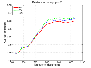
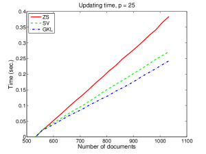
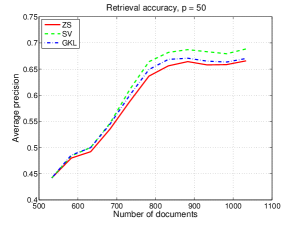
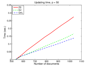
Fig. 1: MEDLINE collection: $m=7,014$, $n=1,033$, $k=75$, $t=533$, $n_{q}=30$. The average precision and time for adding groups of $p=25$ (top) and $p=50$ (bottom) documents. The number of singular triplets of $(I-U_{k}U_{k}^{T})D$ computed by Algorithm 4.1 (“SV”) is $2$ (top) and $4$ (bottom). The number of GKL steps in Algorithm 4.5 (“GKL”) is $3$ (top) and $5$ (bottom). The methods are compared to Algorithm 3.1 (“ZS”).

Figure 1 compares different updating schemes for the MEDLINE collection. This collection is known to be small, with the term-document matrix having $m=7,014$ rows and $n=1,033$ columns. We fix the initial $t=533$ columns and add the rest in groups of $p=25$ (top) and $p=50$ (bottom). The size $k$ of the reduced subspace is set to $75$.

The left-hand side plots demonstrate the differences in the retrieval accuracy. The plots to the right compare the timing results. The horizontal axes represent the number of documents in the collection after consecutive updates. The vertical axes correspond to the mean of the average precisions (left) and the cumulative time (right), i.e., the total time spent by the algorithms to perform the current and preceding updates.

The example demonstrates that the number $l$ of the singular and GKL vectors generated by Algorithms 4.1 and 4.5 can be very small. In particular, we construct as few as 2-3 singular triplets and 3-4 GKL vectors. As anticipated from the discussion in subsection 4.3, this fact gives rise to updating schemes that are significantly faster than the Zha–Simon approach in Algorithm 3.1. Figure 1 (right) confirms that the new strategies in Algorithms 4.1 and 4.5 are indeed considerably faster than the existing scheme. Remarkably, the gain in the efficiency comes without any loss of the retrieval accuracy; see Figure 1 (left).

It can be observed from the figure that Algorithm 4.1 gives the most accurate results though it requires slightly more compute time than Algorithm 4.5. This time difference is caused by the overhead accumulated by the singular value solver to ensure the convergence and perform the extraction of the approximate singular triplets in step 1 of Algorithm 4.1.

# top ranked doc.	10	30	40	70	500	1,000
# rel. doc. (ZS)	7	16	17	20	23	23
# rel. doc. (SV)	10	29	35	38	39	39
pval	0.06	$1.1\times 10^{-4}$	$2.5\times 10^{-5}$	0.002	0.036	0.039

Table 4: MEDLINE collection: the two sample proportion tests for the relevant document counts obtained using Algorithm 3.1 (“ZS”) and Algorithm 4.1 (“SV”).

Note that the number of GKL vectors in Algorithm 4.5 is slightly larger than that of the singular triplets in Algorithm 4.1. This represents a “compensation” for the non-optimal choice of the low-rank approximation of $(I-U_{k}U_{k}^{T})D$ adopted by Algorithm 4.5. Further increase in the number of the GKL vectors may lead to higher retrieval accuracies, but the timing is accordingly affected. The latter observation is true for all of our experiments and is consistent with the relevant results in [8].

In order to yet more carefully compare the retrieval accuracy results, in Table 4 we report numbers of relevant documents (“# rel. doc.”) among the $j$ top ranked (“# top ranked doc.”) for the Zha–Simon (“ZS”) and the new (“SV”) approaches. Here the retrieval is performed from the entire collection ($n=1,033$), after all columns of $A$ have been appended, using the approximate SVD’s generated by the two different updating modes.

The results in Table 4 demonstrate that the new approach gives noticeably larger numbers of relevant document, i.e., a higher precision is obtained at any level $j$. One might debate, however, whether the difference in precision is statistically significant or if it is due to chance alone.

To address this issue we perform a two sample proportion test whose goal is to determine whether or not the difference between two proportions is significant, see, e.g., [27, Chap. 10]. Given the two proportions of relevant documents out of $j$ top ranked, the test has as its null hypothesis that the proportions are drawn from the same binomial distribution. The “pval” values, giving the probability under the null hypothesis, are reported in Table 4. One can observe that these values appear to be very small, not exceeding $0.06$ (for $j=10$) and getting as low as $2.5\times 10^{-5}$ (for $j=40$). Thus, the null hypothesis can be rejected with at least 94% confidence for any level $j$, i.e., the difference in precisions can be seen as statistically significant.

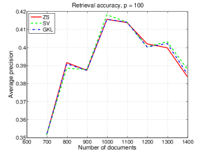
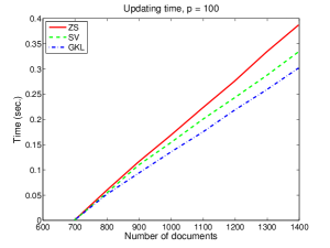
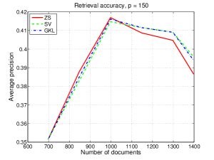
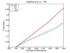
Fig. 2: CRANFIELD collection: $m=3,763$, $n=1,398$, $k=150$, $t=698$, $n_{q}=225$. The average precision and time for adding groups of $p=100$ (top) and $p=150$ (bottom) documents. The number of singular triplets of $(I-U_{k}U_{k}^{T})D$ computed by Algorithm 4.1 (“SV”) is $25$ (top and bottom). The number of GKL steps in Algorithm 4.5 (“GKL”) is 51 (top) and 45 (bottom). The methods are compared to Algorithm 3.1 (“ZS”).

Figure 2 displays the results for the CRANFIELD collection. Similar to MEDLINE, CRANFIELD represents another example of a small text collection, with the term-document matrix having $m=3,763$ rows and $n=1,398$ columns. Following our test framework, we fix the initial $t=698$ columns and add the rest in groups of $p=100$ (top) and $p=150$ (bottom). The dimension $k$ of the reduced subspace is set to $150$.

The number $l$ of singular triplets in Algorithm 4.1 is chosen to be 25 for both values of $p$. The number of GKL steps is set to 51 ($p=100$) and 45 ($p=150$). In contrast to the previous example, smaller values of $l$ fail to deliver acceptable retrieval accuracies. Nevertheless, as can be seen in Figure 2 (right), the new updating schemes are still noticeably faster than Algorithm 3.1. The retrieval accuracy is comparable for all three approaches, and is slightly higher for the new schemes at the later updates.

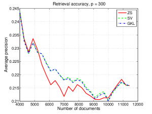
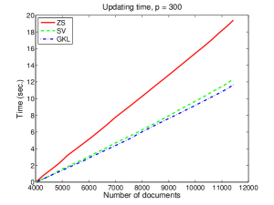
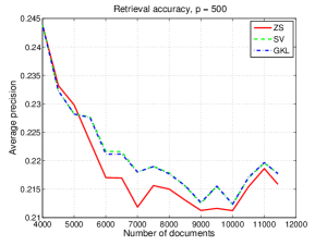
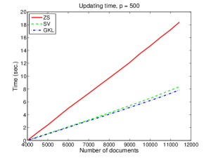
Fig. 3: NPL collection: $m=7,491$, $n=11,429$, $k=550$, $t=4,000$, $n_{q}=93$. The average precision and time for adding groups of $p=300$ (top) and $p=500$ (bottom) documents. The number of singular triplets of $(I-U_{k}U_{k}^{T})D$ computed by Algorithm 4.1 (“SV”) is $10$ (top and bottom). The number of GKL steps in Algorithm 4.5 (“GKL”) is $20$ (top and bottom). The methods are compared to Algorithm 3.1 (“ZS”).

In Figure 3 we report results for the NPL collection. NPL is a larger text collection with the associated term-document matrix having $m=7,491$ rows and $n=11,429$ columns. Note that, in contrast to the previous case, here the number of rows is smaller than the number of columns. In this sense, NPL provides a more representative example of the real-world large-scale text collections, where the number of terms in the vocabulary is limited while the number of documents, in principle, can become arbitrarily large. For the test purposes we fix $t=4,000$ initial columns and add the rest in groups of $p=300$ and $p=500$; $k=550$.

# top ranked doc.	100	500	1,000	11,000
# rel. doc. (ZS)	11	18	21	22
# rel. doc. (SV)	58	72	73	82
pval	$2.7\times 10^{-12}$	$2.4\times 10^{-9}$	$3.9\times 10^{-8}$	$3.7\times 10^{-9}$

Table 5: NPL collection: the two sample proportion tests for the relevant document counts obtained using Algorithm 3.1 (“ZS”) and Algorithm 4.1 (“SV”).

Figure 3 shows that for the NPL dataset the new updating schemes are also faster and deliver a comparable retrieval accuracy. Note that the number $l$ of the singular and GKL vectors is kept reasonably low. In particular, we request 10 singular triplets in step 1 of Algorithm 4.1 and 20 GKL vectors in step 1 of Algorithm 4.5.

In Table 5, we further assess the retrieval accuracy. Similar to Table 4 for the MEDLINE collection, after completing the whole cycle of updates, we present numbers of relevant documents among the $j$ top ranked for the Zha–Simon (“ZS”) and the new (“SV”) approaches. In the same manner, we run the two sample proportion test for each number $j$ of the top ranked documents and report the “pval” values. As in the previous example in Table 4, these values turn out to be very small, suggesting statistical significance of the difference in the precision results.

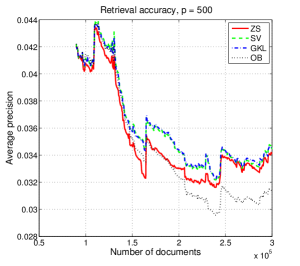
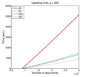
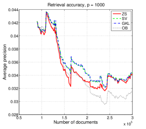
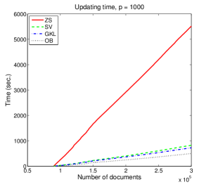
Fig. 4: TREC8 collection: $m=138,232$, $n=528,028$, $k=400$, $t=90,000$, $n_{q}=50$. The average precision and time for adding groups of $p=500$ (top) and $p=1000$ (bottom) documents. The number of singular triplets of $(I-U_{k}U_{k}^{T})D$ computed by Algorithm 4.1 (“SV”) is $10$. The number of GKL steps in Algorithm 4.5 (“GKL”) is $20$. The methods are compared to Algorithm 3.1 (“ZS”) and the updating scheme [3, 19] (“OB”).

Figure 4 concerns a larger example given by the TREC8 dataset. This dataset is known to be extensively used for testing new text mining algorithms. It is comprised of four document collections (Financial Times, Federal Register, Foreign Broadcast Information Service, and Los Angeles Times) from the TREC CDs 4 $\&$ 5 (copyrighted). The queries are from the TREC-8 ad hoc task; see http://trec.nist.gov/data/topics_eng/. The relevance files are available at http://trec.nist.gov/data/qrels_eng/.

After the pre-processing step discussed at the beginning of this section, TREC8 delivers a term-document matrix with total of $m=138,232$ terms and $n=528,028$ documents. In our experiment, we fix the initial $t=90,000$ columns and then incrementally add the new columns in groups of $p=500$ (top) and $p=1,000$ (bottom) until their total number reaches $300,000$. In both cases, the value of $l$ is relatively small: we use only 10 singular triplets and 20 GKL vectors.

As can be seen in Figure 4, the gain in the efficiency presented by the new schemes becomes even more pronounced when the methods are applied to a larger dataset. In particular, our tests show a three-fold speed-up of the overall updating process (420 sequential updates) for $p=500$ and a five-fold speed-up (210 sequential updates) for $p=1,000$. Yet, in both cases, the proposed algorithms deliver a comparable retrieval accuracy.

In Figure 4 we also report the results for schemes [3, 19] (“OB”). As has been previously discussed, these schemes are known to be fast but generally lack accuracy. This is confirmed by our experiment. Remarkably, the methods proposed in this paper are essentially as fast as those in [3, 19], but the accuracy is higher than that of Zha–Simon schemes [29]. Note that in contrast to [3, 19], which can be obtained by setting $l=0$ in our algorithms, the presence of a nonzero number $l$ of singular or GKL vectors is indeed critical for maintaining the accuracy.

6 Conclusion

This paper introduces several new algorithms for the SVD updating problem in LSI. The proposed schemes are based on classical projection methods applied to the singular value computations. A key ingredient of the new algorithms is the construction of low-dimensional search subspaces. A proper choice of such subspaces leads to fast updating schemes with a modest storage requirement.

In particular, we consider two options for reducing the dimensionality of search subspaces. The first one is based on the use of (approximate) singular vectors. The second options utilizes the GKL vectors. Our tests show that generally a larger number of GKL vectors is needed to obtain comparable retrieval accuracy. However, the case of singular vectors has a slightly higher computational cost.

Note that construction of search subspaces is not restricted only to the two techniques considered in the present work. Due to the established link to a Rayleigh-Ritz procedure, other approaches for generating search subspaces can be investigated within this framework in future research.

Our experiments demonstrate a substantial efficiency improvement over the state-of-the-art updating algorithms [29]. While in our tests we have also consistently observed a slight increase in the retrieval accuracy, it is not clear how and if the observed gains are related to the proposed algorithmic developments. This issue should be addressed in future research.

Since the new approach scales linearly in $p$ (in contrast to the cubic scaling exhibited by the existing methods [29]), the efficiency gap becomes especially evident as $p$ increases. Because significantly large values of $p$ are likely to be encountered in the context of large-scale datasets, this means that in the future, algorithms such as the ones proposed in this paper, may play a role in reducing the cost of standard SVD-based techniques employed in the related applications.

References

- [1] R. A. Baeza-Yates and B. A. Ribeiro-Neto, Modern Information Retrieval, ACM Press/Addison-Wesley, 1999.
- [2] M. Berry, Z. Drmac, and E. R. Jessup, Matrices, vector spaces, and information retrieval, SIAM Review, 41 (1999), pp. 335–362.
- [3] M. Berry, S. Dumais, and G. O. Brien, Using linear algebra for intelligent information retrieval, SIAM Review, 37 (1995), pp. 573–595.
- [4] M. W. Berry, SVDPACK: A Fortran-77 software library for the sparse singular value decomposition, tech. rep., Knoxville, TN, USA, 1992.
- [5] C. M. Bishop, Pattern Recognition and Machine Learning, Information Science and Statistics, Springer, 2006.
- [6] K. Blom and A. Ruhe, A Krylov subspace method for information retrieval, SIAM Journal on Matrix Analysis and Applications, 26 (2005), pp. 566–582.
- [7] J. Chen and Y. Saad, Divide and conquer strategies for effective information retrieval, in SIAM Data Mining Conf. 2009, C. Kamath, ed., 2009, pp. 449–460.
- [8] , Lanczos vectors versus singular vectors for effective dimension reduction, IEEE Trans. on Knowledge and Data Engineering, 21 (2009), pp. 1091–1103.
- [9] S. Deerwester, S. Dumais, G. Furnas, T. Landauer, and R. Harshman, Indexing by latent semantic analysis, J. Soc. Inf. Sci., 41 (1990), pp. 391–407.
- [10] I. S. Dhillon and D. S. Modha, Concept decompositions for large sparse text data using clustering, Mach. Learn., 42 (2001), pp. 143–175.
- [11] G. H. Golub and W. M. Kahan, Calculating the singular values and pseudoinverse of a matrix, SIAM J. Num. Anal. Ser. B, 2 (1965), pp. 205–224.
- [12] G. H. Golub and C. F. V. Loan, Matrix Computations, Johns Hopkins University Press, Baltimore, MD, 3rd ed., 1996.
- [13] D. K. Harman, The 3rd text retrieval conference (trec-3), ed. (1995). NIST Special Publication 500-225. http://trec.nist.gov.
- [14] V. Hernández, J. E. Román, and A. Tomás, A robust and efficient parallel SVD solver based on restarted Lanczos bidiagonalization, Electron. Trans. Numer. Anal., 31 (2008), pp. 68–85.
- [15] M. E. Hochstenbach, A Jacobi-Davidson type SVD method, SIAM Journal on Scientific Computing, 23 (2001), pp. 606–628.
- [16] E. Kokiopoulou and Y. Saad, Polynomial Filtering in Latent Semantic Indexing for Information Retrieval, in ACM-SIGIR Conference on research and development in information retrieval, Sheffield, UK, July 25th-29th 2004.
- [17] T. Kolda and D. O. Leary, A semi-discrete matrix decomposition for latent semantic indexing in information retrieval, ACM Transactions on Information Systems, 16 (1998), pp. 322–346.
- [18] J. E. Mason and R. J. Spiteri, A new adaptive folding-up algorithm for information retrieval, 2007.
- [19] G. W. O’Brien, Information management tools for updating an SVD-encoded indexing scheme, 1994. Masters Thesis, Department of Computer Science, University of Tennessee, Knoxville, TN.
- [20] B. N. Parlett, The Symmetric Eigenvalue Problem, no. 20 in Classics in Applied Mathematics, SIAM, Philadelphia, 1998.
- [21] Y. Saad, Numerical Methods for Large Eigenvalue Problems- classics edition, SIAM, Philadelpha, PA, 2011.
- [22] G. Salton, Automatic Text Processing, Addison-Wesley, New York, 1989.
- [23] G. Salton and M. McGill, Introduction to Modern Information Retrieval, McGraw-Hill, New York, 1983.
- [24] H. Simon and H. Zha, Low rank matrix approximation using the Lanczos bidiagonalization process, SIAM J. Sci. Stat. Computing, 21 (2000), pp. 2257–2274.
- [25] J. E. Tougas and R. J. Spiteri, Updating the partial singular value decomposition in latent semantic indexing, Comput. Stat. Data An., 52 (2008), pp. 174–183.
- [26] L. van der Maaten, E. Postma, and H. van den Herik, Dimensionality reduction: A comparative review, Tech. Rep. TiCC-TR 2009-005, Tilburg University, 2009.
- [27] L. Wasserman, All of statistics, Springer texts in statistics, Springer, 2003.
- [28] D. Zeimpekis and E. Gallopoulos, TMG: A MATLAB-based term-document matrix constructor for text collections, tech. rep., Comp. Sci. dept, University of Patras, December 2003.
- [29] H. Zha and H. Simon, On updating problems in latent semantic indexing, SIAM Journal on Scientific Computing, 21 (1999), pp. 782–791.
- [30] H. Zha and H. Zhang, Matrices with low-rank-plus-shift structure: partial SVD and latent semantic indexing, SIAM. J. Matrix Anal. Appl., 21 (2000), pp. 522–536.