FIT HE - 13-01

Ad$S_{5}$ with two boundaries
and holography of $\cal{N}=$4 SYM theory

Kazuo Ghoroku and Masafumi Ishihara, Akihiro Nakamura

^†Fukuoka Institute of Technology, Wajiro, Higashi-ku
Fukuoka 811-0295, Japan
^‡WPI-Advanced Institute for Materials Research (WPI-AIMR), Tohoku University, Sendai 980-8577, Japan

^§Department of Physics, Kagoshima University, Korimoto1-21-35,Kagoshima 890-0065, Japan

According to the AdS/CFT correspondence, the ${\cal N}=4$ supersymmetric Yang-Mills (SYM) theory is studied through its gravity dual whose configuration has two boundaries at the opposite sides of the fifth coordinate. At these boundaries, in general, the four dimensional (4D) metrics are different, then we expect different properties for the theory living in two boundaries. It is studied how these two different properties of the theory are obtained from a common 5D bulk manifold in terms of the holographic method. We could show in our case that the two theories on the different boundaries are described by the Ad$S_{5}$, which is separated into two regions by a domain wall. This domain wall is given by a special point of the fifth coordinate. Some issues of the entanglement entropy related to this bulk configuration are also discussed.

1 Introduction

Up to now, many holographic approaches to the ${\cal N}=4$ supersymmetric Yang-Mills (SYM) theory have been performed in terms of the dual supergravity [1]-[10]. These approaches are based on a conjectured correspondence between a conformal field theory on the boundary M_d of an asymptotic Anti de Sitter space (AdS_d+1) and string theories on the product of AdS_d+1 with a compact manifold. In many cases, the boundary M_d is set as a Minkowski space-time, and the bulk manifolds have a structure that they have a boundary at the ultraviolet (UV) side of the dual d-dimensional CFT. On the other hand, in the infrared side, they have a horizon. Then the holographic analyses for CFT in M_d are performed in the region between the horizon and the boundary for the gravity side.

In these approaches, the research has been extended to the SYM theory in the background of $M_{4}=dS_{4}(AdS_{4})$ by introducing 4D cosmological constant ($\Lambda_{4}>0~{}(\Lambda_{4}<0)$) [11, 12, 13, 14, 15, 16] in the supergravity solutions. In the bulk supergravity solutions, $\Lambda_{4}$ appears as a free parameter in the step of solving the equations of motion. However, this parameter plays an important role since the 4D geometry of the boundary is controlled by this parameter. Another important point is that the form of the bulk metric is also deformed by this parameter. As a result, we could see how the dynamical properties of the SYM theory are changed by the 4D geometry which is changed from the Minkowski space-time to $dS_{4}(AdS_{4})$.

Actually, in the cases of the dS₄ [11, 12] and AdS₄ [13], we find quite different properties of the SYM theory from the one observed in the Minkowsi space-time. For dS₄ background, we observe a horizon in the infrared side of the fifth coordinate and we find the phenomena similar to the one of the finite temperature SYN theory in the deconfinement phase. On the other hand, in the case of $\Lambda_{4}<0$ (for AdS₄ boundary), we could find that the theory is in the confining phase [13]. Further, we found that the meson spectrum obtained in our analysis is consistent with the one obtained in the usual field theory in AdS₄ [23].

Furthermore, we should notice that it is possible to introduce another free parameter in the bulk AdS₅ solution. This parameter is called as the dark radiation, which corresponds to the thermal excitation of SYM fields, plays an important role in determining the (de)confining phase of the theory [14, 15, 16].

Our purpose in this article is to point out and discuss a characteristic holographic feature of the AdS₅ bulk solution. The point is that a second boundary appears in the solution with AdS₄ boundary without horizons. It is found at the ”infrared limit” ($r=0$), which is opposite to the boundary at ”ultraviolet limit” ($r=\infty$). Here $r$ denotes the fifth coordinate of the AdS₅. Then the gravity of the bulk AdS₅ is dual to the two theories living on the two boundaries separately.

We should notice that two boundaries are also seen in the case of the solution with dS₄ boundary. However, in this case, a horizon appears between the boundaries, then we can restrict the region of the holographic dual to the one between the horizon and a boundary to study the dynamical properties of the theory living on the boundary. In the other half region, the same things are considered, however, the physics of the two boundaries might be independent of each other. In the case of AdS₄ boundary, on the other hand, there is no horizon as such a border between the two boundaries

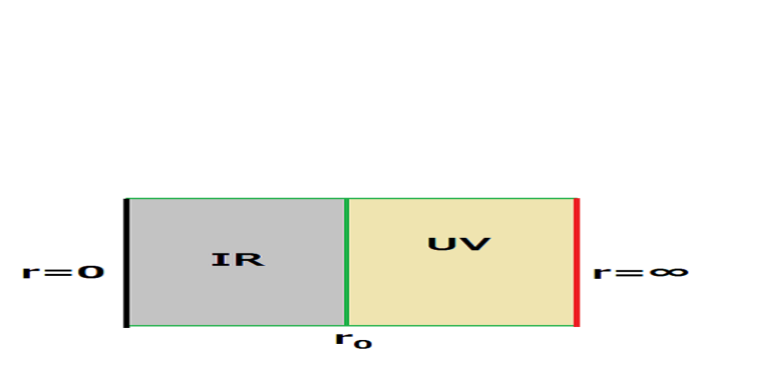
Fig. 1: A schematic picture which represents the bulk ${AdS_{5}}$ with two boundaries (shown by $r=0$ and $r=\infty$). The middle line ($r=r_{0}$) shows the domain wall (horizon) for ${AdS_{4}}$ (${dS_{4}}$) boundary. This line separates the bulk into two regions shown by ”IR” and ”UV”, which are dual to the theory on the boundaries at $r=0$ and $r=\infty$.

The problem in this case (AdS₄ boundary) is how the bulk manifold could provide dynamical properties of the two field theories. In other words, how we could get information of two theories separately from the common bulk geometry. This problem is resolved due to the presence of a sharp domain wall in the bulk. The dynamical properties of the boundary theory are found through various stringy objects embedded in the bulk as probes since the probes are controlled by the bulk configuration which reflects vacuum structure of the dual theory. In the present case, we could find that the embedded objects are confined in one side and never cross the wall to penetrate to the other side. Then, in this sense, the gravity duals for the two boundaries are separated clearly by this wall. Therefore, this wall separates the manifold to two regions which are surrounded by the boundaries at $r=0$ and $r=\infty$ respectively. They correspond to two dual field theories of the two boundaries. The situation is shown in the Fig.1, where the two regions are shown by ”IR” and ”UV”. We would address the holographic problem from this viewpoint and examine the robustness of the wall.

This statement would be correct at the level of classical in the gravity side of the bulk. When we consider the quantum fluctuations of the bulk, they could cross the wall since there is no obstacles to prevent their propagation like a singularity at this wall point. On this problem, we will discuss in a future article.

When we add the dark radiation, our solutions of FRW type are modified. We find that the role of the dark radiation is to shift the position of the horizon and the domain wall for dS₄ and AdS₄ cases respectively. In the latter case, a phase transition from confinement to the deconfinement phase is seen when the magnitude of this term exceeds a critical value as shown in [14]. Another observation is that this term deforms the geometry of IR boundary. On the other hand, the metric at the UV boundary is not affected by the dark radiation. This fact seems to be curious but interesting. We will give more details on this point in the future publication.

In the next section, our model to be examined is given and two boundaries of the gravity dual are shown. Then, in the section 3, we show the existence of the domain wall which devides the bulk region of two boundary theories through the Wilson loop, D7 and D5 embeddings. From these, we can say quarks, flavored mesons and baryons are all separately examined in each bulk region corresponding to the dual theory in each boundary. In the section 4, the entanglement entropy is examined. In this case also, the minimal surface giving the entanglement entropy of a theory in one boundary cannot penetrate into the region which is dual to the other boundary theory since the penetration is protected by the domain wall. This fact implies that there is no entanglement of the two theories of each boundary. Summary and discussions are given in the final section.

2 Setup of the model

First, we briefly review our model [14, 15, 16]. We start from the 10d type IIB supergravity retaining the dilaton $\Phi$, axion $\chi$ and selfdual five form field strength $F_{(5)}$,

$$S={1\over 2\kappa^{2}}\int d^{10}x\sqrt{-g}\left(R-{1\over 2}(\partial\Phi)^{2}+{1\over 2}e^{2\Phi}(\partial\chi)^{2}-{1\over 4\cdot 5!}F_{(5)}^{2}\right),$$ (1)

where other fields are neglected since we do not need them, and $\chi$ is Wick rotated [22]. Under the Freund-Rubin ansatz for $F_{(5)}$, $F_{\mu_{1}\cdots\mu_{5}}=-\sqrt{\Lambda}/2~{}\epsilon_{\mu_{1}\cdots\mu_{5}}$ [20, 21], and for the 10d metric as $M_{5}\times S^{5}$,

$$ds^{2}_{10}=g_{MN}dx^{M}dx^{N}+g_{ij}dx^{i}dx^{j}=g_{MN}dx^{M}dx^{N}+R^{2}d\Omega_{5}^{2}\,,$$

we consider the solution. Here, the parameter is set as $(\mu=)1/R=\sqrt{\Lambda}/2$.

While the dilaton $\Phi$ and the axion $\chi$ play an important role when the bounadary of $M_{5}$ is given by Minkowski space-time [20, 21], we neglect them here since we study the case of (A)dS₄ boundary. Then the equations of motion of non-compact five dimensional part $M_{5}$ are written as

$$R_{MN}=-\Lambda g_{MN}\,.$$ (3)

While this equation leads to the solution of Ad$S_{5}$, there are various Ad$S_{5}$ forms of the solutions which are discriminated by the geometry of their 4D boundary as shown below.

2.1 Solution

A class of solutions of the above equation (3) are obtained in the following form of metric [16],

$$ds^{2}_{10}={r^{2}\over R^{2}}\left(-\bar{n}^{2}dt^{2}+\bar{A}^{2}a_{0}^{2}(t)\gamma_{ij}(x)dx^{i}dx^{j}\right)+\frac{R^{2}}{r^{2}}dr^{2}+R^{2}d\Omega_{5}^{2}\ .$$ (4)

where

$$\gamma_{ij}(x)=\delta_{ij}\left(1+k{\bar{r}^{2}\over 4\bar{r_{0}}^{2}}\right)^{-2}\,,\quad\bar{r}^{2}=\sum_{i=1}^{3}(x^{i})^{2}\,,$$ (5)

and $k=\pm 1,$ or $0$. The arbitrary scale parameter $\bar{r_{0}}$ is set hereafter as $\bar{r_{0}}=1$. For the undetermined non-compact five dimensional part, the following equation is obtained from the $tt$ and $rr$ components of (3) [18, 19],

$$\left({\dot{a}_{0}\over a_{0}}\right)^{2}+{k\over a_{0}^{2}}=-{\Lambda\over 4}A^{2}+\left({{r\over R}A^{\prime}}\right)^{2}+{C\over a_{0}^{4}A^{2}}\ ,$$ (6)

where $\dot{a_{0}}=\partial a_{0}/\partial t$, $A^{\prime}=\partial A/\partial r$, and

$$A={r\over R}\bar{A},\quad{\partial_{t}({a_{0}(t)A})\over\dot{a}_{0}(t)}={r\over R}\bar{n}\,.$$ (7)

The constant $C$ is given as an integral constant in obtaining (6), and we could understand that it corresponds to the thermal excitation of ${\cal N}=4$ SYM theory for $a_{0}(t)=1$, and it is called as dark radiation [18, 19].

At this stage, two undetermined functions, $\bar{A}(r,t)$ and $a_{0}(t)$, are remained. textcolorredHowever the equation to solve them is the Eq.(6) only. Therefore, we could determine $a_{0}(t)$ by introducing the 4D Friedmann equation, which is independent of (3). However it should be realized on the boundary where various kinds of matter could be added in order to form the presumed FRW universe as in [16]

$$\left({\dot{a}_{0}\over a_{0}}\right)^{2}+{k\over a_{0}^{2}} = {\Lambda_{4}\over 3}+{\kappa_{4}^{2}\over 3}\left({\rho_{m}\over a_{0}^{3}}+{\rho_{r}\over a_{0}^{4}}+{\rho_{u}\over a_{0}^{3(1+u)}}\right)\equiv\lambda(t)\,$$ (8)

where $\kappa_{4}$ ($\Lambda_{4}$) denotes the 4D gravitational constant (cosmological constant). The quantities $\rho_{m}$ and $\rho_{r}$ denote the energy density of the nonrelativistic matter and the radiation of 4D theory respectively. The most right hand side expression $\lambda(t)$ in (8) is given as a simple form of the most left hand side of (8) given by using $a_{0}(t)$. Then the remaining function $A(t,r)$ is obtained from (6) in terms of $\lambda(t)$. The last term $\rho_{u}$ in the middle of (8) represents an unknown matter with the equation of state, $p_{u}=u\rho_{u}$, where $p_{u}$ and $\rho_{u}$ denote its pressure and energy density respectively. It is important to be able to solve the bulk equation (6) in this way by relating its left hand side to the Friedmann equation defined on the boundary [16] since we could have a clear image for the solution.

Finally, the solution is obtained as

$$\bar{A} = \left(\left(1-{\lambda\over 4\mu^{2}}\left({R\over r}\right)^{2}\right)^{2}+\tilde{c}_{0}\left({R\over r}\right)^{4}\right)^{1/2}\,,$$ (9)

$$\bar{n} = {\left(1-{\lambda\over 4\mu^{2}}\left({R\over r}\right)^{2}\right)\left(1-{\lambda+{a_{0}\over\dot{a}_{0}}\dot{\lambda}\over 4\mu^{2}}\left({R\over r}\right)^{2}\right)-\tilde{c}_{0}\left({R\over r}\right)^{4}\over\sqrt{\left(1-{\lambda\over 4\mu^{2}}\left({R\over r}\right)^{2}\right)^{2}+\tilde{c}_{0}\left({R\over r}\right)^{4}}}\,,$$ (10)

where

$$\tilde{c}_{0}=C/(4\mu^{2}a_{0}^{4})\,.$$ (11)

2.2 Two boundaries

Urtraviolet boundary $r\to\infty$

In the case of the above solution, there is a boundary at $r\to\infty$, where the energy scale of the dual field theory is at the ultraviolet limit. The boundary should be set at the position where the metric has a second order pole [24] since the manifold is not well defined there. At this boundary $r\to\infty$, the 4D metric is given as

$$ds_{\rm FRW}^{2}=-dt^{2}+a_{0}(t)^{2}\gamma_{ij}dx^{i}dx^{j}\,,$$ (12)

since the above solution behaves as $\bar{n}\to 1$ and $\bar{A}(r,t)\to 1$ for $r\to\infty$. This is the well-known Friedmann-Robertson-Walker (FRW) metric, which is usually used in cosmology to study the time development of our universe. In the present case, therefore, we can study the SYM theory in this FRW universe from the bulk metric (4) which is the holographic dual as shown in [16].

Infrared boundary $r\to 0$

Next, from (9) and (10), we find that there is another boundary at $r\to 0$, in the infrared limit, for $\Lambda_{4}<0$, small $C$ and tiny time dependence of $\lambda(t)$. However the appearance of this boundary depends on the time when the effect of $C$ and time dependence of $\lambda(t)$ are considered. The situation is therefore a little complicated. For example, consider the case of $\dot{\lambda}=0$ for simplicity, then the second boundary is found for $\lambda<0$ and $|{\lambda\over 4\mu^{2}}|>\sqrt{\tilde{c}_{0}}$. However, the last inequality depends on time and it is satisfied for restricted time-interval. So more simple case is considered below.

i) For the case of $C=0$ and negative constant $\lambda(=-\lambda_{0})$

In order to make clear the two boundaries, the situation is simplified by considering the case of $\lambda=-\lambda_{0}$ and $C=0$, where $\lambda_{0}$ is a positive constant. This is corresponding to the case of negative $\Lambda_{4}$ and $\lambda_{0}=-\Lambda_{4}/3$. In this case, the scale factor is given by solving Eq.(8) for $k=-1$ as follows,

$$a_{0}(t)=\sin\left(\sqrt{\lambda_{0}}t\right)/\sqrt{\lambda_{0}}$$ (13)

and then the metric is written as

$$ds^{2}_{10} = ds^{2}_{5}+R^{2}d\Omega_{5}^{2}$$ (14)

$$ds^{2}_{5} = {r^{2}\over R^{2}}\left(1+{r_{0}^{2}\over r^{2}}\right)^{2}\left(-dt^{2}+a_{0}^{2}(t)\gamma_{ij}(x)dx^{i}dx^{j}\right)+\frac{R^{2}}{r^{2}}dr^{2}$$ (15)

where $r_{0}^{2}=\lambda_{0}R^{4}/4$ and

$$\gamma_{ij}(x)=\delta_{ij}\left(1-{\bar{r}^{2}\over 4}\right)^{-2}\,.$$ (16)

In this case, the boundary represents a typical AdS₄ manifold, and the SYM theory on this manifold has been holographically examined well previously [13]. In this case, the analysis has been performed by supposing that the bulk is dual to the theory on the boundary $r=\infty$. And we have paid no attention to the other possible boundary at $r=0$.

However, in order to have correct results of the analysis, we must notice the fact that there is actually another boundary at $r\to 0$ in the bulk of (19). In order to see this point clearly, we rewrite the above metric by changing the coordinate $r$ as $r=r_{0}^{2}/z$, then we have

$$ds^{2}_{10}={z^{2}\over R^{2}}\left(1+{r_{0}^{2}\over z^{2}}\right)^{2}\left(-dt^{2}+a_{0}^{2}(t)\gamma_{ij}(x)dx^{i}dx^{j}\right)+\frac{R^{2}}{z^{2}}dz^{2}+R^{2}d\Omega_{5}^{2}\ .$$ (17)

Then we find again the same form of metric with (19), but $r$ is replaced by $z$. This implies the following two points. (i) There must be another bulk region near $z=\infty$ which is dual to SYM theory living on $AdS_{4}$ at $z=\infty$. (ii) Secondly, the limit of $z=\infty$ is also the urtaviolet region of the SYM theory as understood from the form of (17). Then we could obtain the same dynamical information, from the metric (17), of the theory with the one given for the theory at $r=\infty$. In other words, in the bulk manifold, the same two dual theories should be expressed by two regions which are separated at some point of the coordinate $r$. This point is called as domain wall, and we could find it at $r=r_{0}$ as shown below.

ii) For the case of $C=0$ and positive constant $\lambda=\lambda_{0}$

In the case of $\lambda=\lambda_{0}>0$, $\Lambda_{4}$ is positive and the scale factor is given by solving Eq.(8) for $k=0$ as follows,

$$a_{0}(t)=a(0)e^{\sqrt{\lambda_{0}}t}\,,$$ (18)

and then the metric is written as

$$ds^{2}_{10} = d\tilde{s}^{2}_{5}+R^{2}d\Omega_{5}^{2}$$ (19)

$$d\tilde{s}^{2}_{5} = {r^{2}\over R^{2}}\left(1-{r_{0}^{2}\over r^{2}}\right)^{2}\left(-dt^{2}+a_{0}^{2}(t)\delta_{ij}(x)dx^{i}dx^{j}\right)+\frac{R^{2}}{r^{2}}dr^{2}\,.$$ (20)

In this case, the boundary represents dS₄ manifold, and the SYM theory on this manifold has been holographically examined well previously [12] for the theory on the boundary $r=\infty$. And we have considred only for the half region of $r_{0}<r<\infty$, then no attention is paid to the other possible boundary at $r=0$. In this case, however, the situation is different from the above case, and it would be reasonable to restrict to the region $r_{0}<r<\infty$ since the point $r=r_{0}$ represent the horizon. The situation is similar to the case of the Schwartzschild-AdS background, where the holographic region is restricted to the region from the horizon to $r=\infty$.

It would be an interesting problem to study the theory ar $r=0$ boundary by considering the region of $0<r<r_{0}$. We expect similar behaviour to the theory on $r=\infty$. However, here, we give such study in the future article.

iii) General case of $C\neq 0$

Here we consider the metric of general case of $C\neq 0$, namely (4) with (9)-(11). In this case, we find $\bar{A}\neq\bar{n}$ since $\bar{A}$ and $\bar{n}$ are modified by the term $\tilde{c}$ , and $\bar{n}$ could have a zero point as in the case of the black hole configuration when $\tilde{c}$ exceeds a critical value. Then we could find a phase transition by adding the term $C$ to the solution with AdS₄ boundary [14].

In the confinement phase, we find the position of the domain-wall is pushed to $r=0$ by increasing $\tilde{c}$. In the case of dS₄ boundary, the horison is pushe toward to larger $r$. In any case, the boundary metric at $r=0$ is deformed. This point is seen as follows. The five dimensional part of the metric is rewritten in terms of ${z^{*}}=1/z^{2}$ as follows

$$ds^{2}_{(5)}=R^{2}\left({1\over z^{*}}\hat{g}_{\mu\nu}dx^{\mu}dx^{\nu}+{d{z^{*}}^{2}\over 4{z^{*}}^{2}}\right)\,,$$ (21)

and the 4D part is expanded by the powers of $z$ for $R=1$, as follows

$$\hat{g}_{\mu\nu}=\hat{g}_{(0)\mu\nu}+\hat{g}_{(2)\mu\nu}z^{*}+{{z^{*}}^{2}}\left(\hat{g}_{(4)\mu\nu}+\hat{h}_{1(4)\mu\nu}\log z^{*}+\hat{h}_{2(4)\mu\nu}(\log z^{*})^{2}\right)+\cdots\,.$$ (22)

The first term is given as

$$\hat{g}_{(0)\mu\nu} = (\hat{g}_{(0)00},~{}\hat{g}_{(0)ij})\,$$ (23)

$$= \left(-{\left(({b}{b}_{1})^{2}-\tilde{c}_{0}\right)^{2}\over\left({b}^{4}+\tilde{c}_{0}\right)r_{0}^{4}},~{}{{b}^{4}+\tilde{c}_{0}\over r_{0}^{4}}a_{0}(t)^{2}\gamma_{i,j}\right)\,,$$

where

$${b}^{2}=-{\lambda\over 4}R^{4}\,,\quad{b}_{1}^{2}=-{\lambda+\dot{\lambda}a_{0}/\dot{a}_{0}\over 4}R^{4}\,$$ (24)

This implies that the boundary metric depends on the dark radiation, namely the SYM fields. Then this fact seems to be contradict with the expectation of the decoupling of SYM theory and the gravity on the boundary. On the other hand, at the $r=\infty$, the boundary metric is not affected by this dark radiation $C$ as expected. Then the holographic situation is modified in the side of $r=0$ for $C\neq 0$, where the dual 4D theory couples with gravity through the energy momentum tensor generated in the side of SYM theory. It is an interesting problem to make clear this point and to investigate the holography of a SYM theory coupled with the gravity. We however postpone to investigate this problem to the future, and we restrict to the case of $C=0$ hereafter.

3 Gravity dual and domain wall

We consider the gravity dual of the two theories living on different boundaries. It is represented by a common bulk manifold. We study how we can see the holographic properties of two field theories on the same bulk manifold through various objects which are responsible for field theories.

3.1 Wilson-Loop and Quark Confinement

The potential between quark and anti-quark is studied by the Wilson-Loop. It is obtained holographically from the U-shaped ( in $r-x$ plane) string which is embedded in the bulk and its two end-points are on the boundary. Supposing a string whose world volume is set in $(t,x)$ plane , the energy $E$ of this state is obtained as a function of the distance ($L$) between the qaurk and anti-quark according to [12].

Taking the gauge as $X^{0}=t=\tau$ and $X^{1}=x^{1}=\sigma$ for the coordinates $(\tau,~{}\sigma)$ of string world-volume, the Nambu-Goto Lagrangian in the present background (4) becomes

$$L_{\textrm{\scriptsize NG}}=-{1\over 2\pi\alpha^{\prime}}\int d\sigma~{}{\bar{n}(r)}\sqrt{r^{\prime}{}^{2}+\left({r\over R}\right)^{4}\left({\bar{A}(r)}a_{0}(t)\gamma(x)\right)^{2}},$$ (25)

where

$$\gamma(x)={1\over 1-x^{2}/4}\,,$$ (26)

and we notice $r^{\prime}=\partial r/\partial x=\partial r/\partial\sigma$. and $\bar{n},\bar{A}$ have no time dependence since we here use the metric (20). The general form of the solution for $\bar{n}$ and $\bar{A}$ are given in (9)-(11), and they depend on the time through the scale factor $a_{0}(t)$. Then, in order to see the static energy as $E=-L_{\textrm{\scriptsize NG}}$, we should restrict the solutions to the case of $C=0$ and $\lambda=-\lambda_{0}$. In this case, the two boundaries have the same form of metric as given in (19)-(16) and (17) with different notation of the radial coordinate for each boundary, $r$ and $z$ respectively.

In the case of (19)-(16), the energy is rewritten to a more convenient form by introducing the factor $n_{s}$ (given below) [17] as

$$E=-L_{\rm NG}={1\over 2\pi\alpha^{\prime}}\int d\tilde{\sigma}~{}n_{s}~{}\sqrt{1+\left({R^{2}\over r^{2}\bar{A}}\partial_{\tilde{\sigma}}r\right)^{2}}\ ,$$ (27)

$$\tilde{\sigma}=a_{0}(t)\int d\sigma\gamma(\sigma)=a_{0}(t)\int d\sigma{1\over 1-\sigma^{2}/4}\,,$$ (28)

$$n_{s}=\left({r\over R}\right)^{2}\bar{A}\bar{n}=\left({r\over R}\right)^{2}\left(1+{r_{0}^{2}\over r^{2}}\right)^{2}\,,$$ (29)

Here, we use the proper coordinate $\tilde{\sigma}$ instead of the comoving coordinate ${\sigma}$ to measure the distance between the quark and anti-quark.

In this form, the criterion of the confinement is stated such that $n_{s}$ has a finite minimum value at some appropriate $r(=r^{*})$. In the present case, we find $r^{*}=r_{0}$. Actually, in such a case, $E$ is approximated as [12]

$$E\sim{n_{s}(r^{*})\over 2\pi\alpha^{\prime}}{L}\ ,$$ (30)

where

$${L}=2\int_{\tilde{\sigma}_{min}}^{\tilde{\sigma}_{max}}d\tilde{\sigma}\,,$$ (31)

and $\tilde{\sigma}_{min}$ ($\tilde{\sigma}_{max}$) is the value at $r_{min}$ ($r=\infty$) of the string configuration [13]. The tension of the linear potential between the quark and anti-quark is therefore given as

$$\tau_{q\bar{q}}={n_{s}(r_{0})\over 2\pi\alpha^{\prime}}\,.$$ (32)

We notice that the U-shaped string configuration whose bottom point is near $r_{0}$ and the string on both sides goes up toward the boundary $r=\infty$. When the bottom approaches to $r_{0}$ the length $L$ goes to $\infty$. In other words, the string configuration is bounded at $r=r_{0}$ and cannot exceed this point to smaller $r$.

In the case of (17), the procedure of the calculation of the Wilson loop is completely parallel to the above case only by replacing $r$ by $z$. Then we find the same tension of the linear potential between the quark and anti-quark, which are living on the boundary $r=0$ or $z=\infty$, is obtained as

$$\tau_{q\bar{q}}={n_{s}(r_{0})\over 2\pi\alpha^{\prime}}\,.$$ (33)

In the present case, the string on both sides goes up toward the boundary, namely to $r=0$. So the U-shaped configuration of the string has a form which has been upside-down the one obtained above. Then we will find two types of string configurations which are responsible to the Wilson loop calculation. The end points of the one type of string go towards $r=\infty$, and the one of the other type goes to $r=0$. This equation is very complicated, so we show its numerical result in the Fig.2

String configurations and Domain Wall

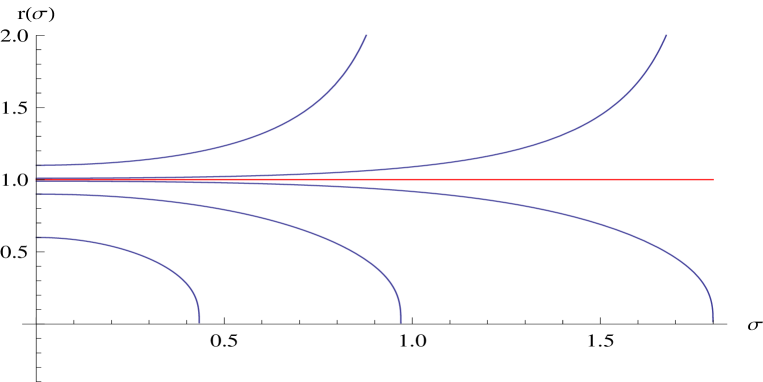
Fig. 2: Solutions for $r(\sigma)$, where $\tilde{\sigma}$ is denoted by $\sigma$. The curves denote for $r(0)=1.1,~{}1.01,~{}0.99,~{}0.9,~{}0.6$ from the above one. The horizontal line $r=1.0$ shows the domain wall.

Here we show the string configurations mentioned above to make clear the situation. They are obtained by solving the equation of motion for the profile of the string. Both the solutions belonging to the boundary $r=\infty$ and $r=0$ are obtained by solving the same equation, which is given from (25) as follows

$$r^{\prime\prime}-r^{\prime}\left(\log\left({r^{4}\over R^{4}}+\left({r^{\prime}\over(1+(r_{0}/r)^{2})}\right)^{2}\right)\right)^{\prime}+2{r_{0}^{3}\over r^{3}}{{r^{\prime}}^{2}\over 1+(r_{0}/r)^{2}}-2{r^{3}\over R^{4}}\left(1-\left({r_{0}\over r}\right)^{4}\right)=0\,$$ (34)

where prime denote the differation with respect to $\tilde{\sigma}$ as $r^{\prime}=\partial_{\tilde{\sigma}}r$. This equation is complicated, so we solve it numerically,

Several configurations are shown in the Fig.2, from which we can see the solutions are separated to two groups by the boundary condition at $\sigma=x=0$, namely the value of $r(0)$. The wall which separate two classes of the solutions is found at $r(0)=r_{0}$.

3.2 D7 brane embedding and domain wall

Here, we study the D7 brane embedding, which is responsible for studying the meson spectrum and the chiral condensate of the boundary theory. The D7-brane action is given by the Dirac-Born-Infeld (DBI) and the Chern-Simons (CS) terms as follows,

$$S_{D7} = -T_{7}\int d^{8}\xi e^{-\Phi}\sqrt{-\det\left(g_{ab}+2\pi\mbox{$\alpha^{\prime}$}F_{ab}\right)}+T_{7}\int\sum_{i}\left(e^{2\pi\mbox{$\alpha^{\prime}$}F_{(2)}}\wedge c_{(a_{1}\ldots a_{i})}\right)_{0\ldots 7}~{},$$ (35)

$$g_{ab} \equiv \partial_{a}X^{\mu}\partial_{b}X^{\nu}G_{\mu\nu}~{},\qquad c_{a_{1}\ldots a_{i}}\,\equiv\,\partial_{a_{1}}X^{\mu_{1}}\ldots\partial_{a_{i}}X^{\mu_{i}}C_{\mu_{1}\ldots\mu_{i}}~{}.$$

where $T_{7}$ is the brane tension. The DBI action involves the induced metric $g_{ab}$ and the $U(1)$ world volume field strength $F_{(2)}=dA_{(1)}$.

Near $r=\infty$

For the simplicity, we consider the background (19) - (20) near the boundary $r=\infty$. The metric of the extra six dimensional part of this metric is rewritten as follows

$$\frac{R^{2}}{r^{2}}dr^{2}+R^{2}d\Omega_{5}^{2}=\frac{R^{2}}{r^{2}}\left(d\rho^{2}+\rho^{2}d\Omega_{3}^{2}+\sum_{i=8}^{9}{dX^{i}}^{2}\right)\,,$$ (36)

where the new coordinate $\rho$ is introduced instead of $r$ with the relation

$$r^{2}=\rho^{2}+(X^{8})^{2}+(X^{9})^{2}$$ (37)

Thus, the induced metric of the D7 brane is obtained as

$$ds^{2}_{8}={r^{2}\over R^{2}}\left(1+{r_{0}^{2}\over r^{2}}\right)^{2}\left(-dt^{2}+a_{0}^{2}(t)\gamma^{2}(x)(dx^{i})^{2}\right)+\frac{R^{2}}{r^{2}}\left((1+{w^{\prime}}^{2})d\rho^{2}+\rho^{2}d\Omega_{3}^{2}\right)\,,$$ (38)

where the profile of the D7 brane is taken as $(X^{8},X^{9})=(w(\rho),0)$ and $w^{\prime}=\partial_{\rho}w$, then

$$r^{2}=\rho^{2}+{w}^{2}\,.$$ (39)

In the present case, there is no R-R filed, so the action is given only by the one of DBI as

$$S_{D7}=-T_{7}\Omega_{3}\int d^{4}xa_{0}^{3}(t)\gamma^{3}(x)\int d\rho\rho^{3}\bar{A}^{4}\sqrt{1+{w^{\prime}}^{2}(\rho)}\,,$$ (40)

where

$$\bar{A}=\left(1+{r_{0}^{2}\over r^{2}}\right)^{2}$$ (41)

and $\Omega_{3}$ denotes the volume of $S^{3}$ of the D7’s world volume.

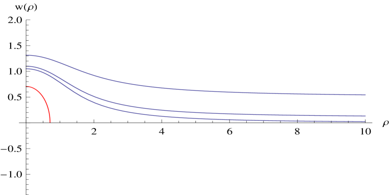
Fig. 3: Typical solutions of $w(\rho)$ for $\lambda_{0}=2,~{}\mu=1/R=1.0$, $r_{0}=1/\sqrt{2}$. The curves are given for $w(0)=1.3,~{}1.1,~{}1.05$ from the above one to the below. The circle represents $r=\sqrt{r_{0}^{2}-\rho^{2}}$, which corresponds the domain wall of the dual bulk manifold for two boundaries.

From this action, the equation of motion for $w$ is obtained as

$$w^{\prime\prime}+\left({3\over\rho}+{\rho+ww^{\prime}\over r}\partial_{r}(\log(\bar{A}^{4}))\right)w^{\prime}(1+{w^{\prime}}^{2})-{w\over r}(1+{w^{\prime}}^{2})^{2}\partial_{r}(\log(\bar{A}^{4}))=0\,.$$ (42)

The constant $w$ is not the solution of this equation, so the supersymmetry is broken. The numerical solutions of (42) for $w(\rho)$ are shown in the Fig. 3. In general, in this case, we find finite chiral condensate $\langle\bar{\Psi}\Psi\rangle=c$ for any $m_{q}\geq 0$ since the curves decrease from the above with increasing $\rho$. For all curves, we find the behavior given by the following asymptotic form

$$w=m_{q}+{c+4m_{q}^{2}r_{0}^{2}\log(\rho)\over\rho^{2}}+\cdots\,,$$ (43)

at large $\rho$ with $c>0$. Here, the term proportional to $\log(\rho)$ comes from the breaking of the conformal invariance due to the cosmological constant in the theory [11, 12, 13]. We can observe spontaneous chiral symmetry breaking from the third curve, which corresponds to $m_{q}=0$. It shows the mass generation of a massless quark due to the chiral condensate $\langle\bar{\Psi}\Psi\rangle$.

As a result, we could say that the spontaneous mass generation of massless quarks is realized in the theory on the boundary at $r=\infty$. This point is already found previously [16]. We notice here that the embedded region of D7 brane with $m_{q}\geq 0$ is restricted to the region $r>r_{0}$. Furthermore, there is no D7 brane configuration which crosses the domain wall $r=r_{0}$ in $w-\rho$ plane. Then the quarks introduced in the dual SYM theory on the boundary $r=\infty$ can be represented by the D7 brane embedded in the region of $r>r_{0}$.

Near $r=0$

For the flavor brane near $r=0$, its embedding is performed as follows. First, by adopting the bulk metric (17), the procedure is completely parallel to the above case by replacing $r$ by $z$. Then the embedded D7 branes of $m_{q}\geq 0$ are all obtained in the region of $z>r_{0}$ and we find the dual theory with chiral symmetry breaking phase at the boundary $r=0$. In the present case, the region $z>r_{0}$ means $r<r_{0}$ since $z=r_{0}^{2}/r$. Then we find the fact that each theory in two boundaries of the bulk is separated by the wall at $r=r_{0}$. Namely, we can study each dual theories can be given by considering the gravity within each region.

3.3 D5 Branes and Baryon

Next, we consider the baryon. It is constructed from a vertex and $N_{c}$ quarks, and the latter are expressed by fundamental strings. The vertex is identified with the D5 brane, which is embedded in the bulk as a probe with a non-trivial $U(1)$ flux in it. Then a baryon is discussed through the D5 brane embedding given as follows.

First, we briefly review the model based on type IIB superstring theory [30, 31, 32, 33, 34]. In the type IIB model, the vertex is described by the D5 brane which wraps $S^{5}$ of the 10D manifold $M_{5}\times S^{5}$. In this case, in the bulk, there exists the following form of self-dual Ramond-Ramond field strength

$$G_{(5)} \equiv dC_{(4)}={4\over R}\left(\epsilon_{S^{5}}+{}^{*}\epsilon_{S^{5}}\right)\,$$ (44)

$$\epsilon_{S^{5}} = R^{5}\,\mbox{vol}(S^{5})d\theta_{1}\wedge\ldots\wedge d\theta_{5}$$ (45)

where $\mbox{vol}(S^{5})\equiv\sin^{4}\theta_{1}\mbox{vol}(S^{4})\equiv\sin^{4}\theta_{1}\sin^{3}\theta_{2}\sin^{2}\theta_{3}\sin\theta_{4}$, and $\epsilon_{S^{5}}$ denotes the volume form of $S^{5}$ part. The flux from the stacked D3 branes flows into the D5 brane as $U(1)$ field which is living in the D5 brane.

The effective action of D5 brane is given by using the Born-Infeld and Chern-Simons term as follows

$$S_{D5} = -T_{5}\int d^{6}\xi e^{-\Phi}\sqrt{-\det\left(g_{ab}+2\pi\mbox{$\alpha^{\prime}$}F_{ab}\right)}+T_{5}\int\left(2\pi\mbox{$\alpha^{\prime}$}F_{(2)}\wedge c_{(4)}\right)_{0\ldots 5}~{},$$ (46)

$$g_{ab} \equiv \partial_{a}X^{\mu}\partial_{b}X^{\nu}G_{\mu\nu}~{},\qquad c_{a_{1}\ldots a_{4}}\,\equiv\,\partial_{a_{1}}X^{\mu_{1}}\ldots\partial_{a_{4}}X^{\mu_{4}}C_{\mu_{1}\ldots\mu_{4}}~{}.$$

where $T_{5}=1/(\mbox{$g_{s}$}(2\pi)^{5}\mbox{$l_{s}$}^{6})$ and $F_{(2)}=dA_{(1)}$, which represents the $U(1)$ worldvolume field strength. In terms of (the pullback of) the background five-form field strength $G_{(5)}$, the above action can be rewritten as

$$S_{D5}=-T_{5}\int d^{6}\xi~{}e^{-\Phi}\sqrt{-\det(g+F)}+T_{5}\int A_{(1)}\wedge G_{(5)}~{},$$

The embedding of the D5 brane is performed by solving the $r(\theta)$, $x(\theta)$, and $A_{(1)}(\theta)$ [34]. They are retained as dynamical fields in the D5 brane action as the function of $\theta\equiv\theta_{1}$ only. The equation of motion for the gauge field $A_{(1)}$ is written as

$$\partial_{\theta}D=-4\sin^{4}\theta,$$

where the dimensionless displacement is defined as the variation of the action with respect to $E=F_{t\theta}$, namely $D=\delta\tilde{S}/\delta F_{t\theta}$ and $\tilde{S}=S/T_{5}\Omega_{4}R^{4}$. The solution to this equation is

$$D\equiv D(\nu,\theta)=\left[{3\over 2}(\nu\pi-\theta)+{3\over 2}\sin\theta\cos\theta+\sin^{3}\theta\cos\theta\right].$$ (47)

Here, the integration constant $\nu$ is expressed as $0\leq\nu=k/N_{c}\leq 1$, where $k$ denotes the number of Born-Infeld strings emerging from one of the pole of the ${\bf S}^{5}$.

Next, it is convenient to eliminate the gauge field in favor of $D$, then the Legendre transformation is performed for the original Lagrangian to obtain an energy functional as [32, 33, 34]:

$$U={N\over 3\pi^{2}\alpha^{\prime}}\int d\theta~{}\bar{n}\sqrt{r^{2}+r^{\prime 2}+(r/R)^{4}x^{\prime 2}(\bar{A}a_{0}\gamma)^{2}}\,\sqrt{V_{\nu}(\theta)}~{}.$$ (48)

$$V_{\nu}(\theta)=D(\nu,\theta)^{2}+\sin^{8}\theta$$ (49)

where we used $T_{5}\Omega_{4}R^{4}=N/(3\pi^{2}\alpha^{\prime})$, and we use the metric form (4). Then, in this expression, (48), $r(\theta)$ and $x(\theta)$ are remained, and they are solved by minimizing $U$. As a result, the D5 brane configuration is determined.

For the simplicity, here, we restrict to the point like configuration, namely $r$ and $x$ are constants. Further, the simple metric (20) is adopted. In this case, we have for the matter considered here

$$U=~{}r\bar{n}(r)U_{0}=r\left(1+{r_{0}^{2}\over r^{2}}\right)U_{0}\,,$$ (50)

where $U_{0}$ is a constant given as

$$U_{0}={N\over 3\pi^{2}\alpha^{\prime}}\int d\theta\sqrt{V_{\nu}(\theta)}~{}.$$ (51)

From (50), we find that $U$ has a minimum at $r_{m}=r_{0}$. Then the vertex is trapped at the domain wall.

We notice, however, the embedded region of the fundamental strings, quarks, are separated to two regions by the domain wall. Namely, the strings cannot cross the domain wall. In this sense, the baryons are also separated to two theories by the wall in the gravity side.

4 Entanglement Entropy and domain wall

Next, we consider the entanglement entropy for the theory of one boundary. It is given by calculating the minimum area of the surface $A$ whose boundary $\partial A$ is set at the boundary of the bulk and the surface could be extended in the bulk. In this calculation, there is a possibility that the minimal surface could penetrate into the bulk region corresponding to the theory living in the other boundary. When this situation is realized, we could see a new entanglement of two theories which are living in the separated boundaries.

In order to see such phenomenon, we estimate the entanglement entropy of a theory in one boundary according to the formula (3.3) in [35]

$$S_{EE}={{\rm Area(\gamma_{A})}\over{4G_{N}^{(5)}}}\,,$$ (52)

where $\gamma_{A}$ denotes the minimal surface, whose boundary is defined by $\partial A$ and the surface is extended into the bulk. And $G_{N}^{(5)}=G_{N}^{(10)}/(\pi^{3}R^{5})$ denotes the 5D newton constant reduced from the 10D one $G_{N}^{(10)}$. If, in this calculation, the minimal surface crosses the domain wall, then we can say that a new kind of an entanglement between two theories on each boundary may exist. This is because the surface or equivalently the entanglement entropy is controlled by the dynamics of the other theory.

We adopt (17) as the bulk metric, which is given as

$$ds^{2}_{10}={z^{2}\over R^{2}}\left(1+{r_{0}^{2}\over z^{2}}\right)^{2}ds^{2}_{FRW_{4}}+\frac{R^{2}}{z^{2}}dz^{2}+R^{2}d\Omega_{5}^{2}\ .$$ (53)

where

$$ds^{2}_{FRW_{4}}=-dt^{2}+a_{0}^{2}(t)\gamma^{2}\left(dp^{2}+p^{2}d\Omega_{2}^{2}\right)\,,$$ (54)

$$p={\bar{r}\over\bar{r}_{0}}\,,\quad\gamma=1/(1-p^{2}/4)\,,$$ (55)

We notice here that the mass dimension is -1 for $a_{0}$, but $p$ has no mass dimension since it is scaled by $\bar{r}_{0}$. In order to study the entanglement entropy (EE), we separate the 3D space of the boundary at a fixed time by a constant value for $p=p_{0}$. Then the EE for the restricted space $p<p_{0}$ is obtained holographically by finding the minimum value of the following quantity

$${S_{\rm area}\over 4\pi} = \left({r_{0}\over R}a_{0}\right)^{3}{\int^{\epsilon}_{x_{0}}}dxf_{1}(x)\,$$ (56)

$$f_{1}(x) = p^{2}\left({1+x^{2}\over x}\right)^{3}\gamma^{3}\sqrt{{p^{\prime}}^{2}+{b\over\gamma^{2}(1+x^{2})^{2}}}\,$$ (57)

$$b = {R^{4}\over a_{0}^{2}r_{0}^{4}}\,,\quad p^{\prime}={\partial p\over\partial x}\,,$$ (58)

where $x=z/r_{0}$, and $x_{0}$ denotes the end point of the embedded surface. Since this integral diverges at the ultraviolet (UV) limit, the UV cutoff $\epsilon$ is introduced. This represents the minimal surface of the ball embedded in the bulk.

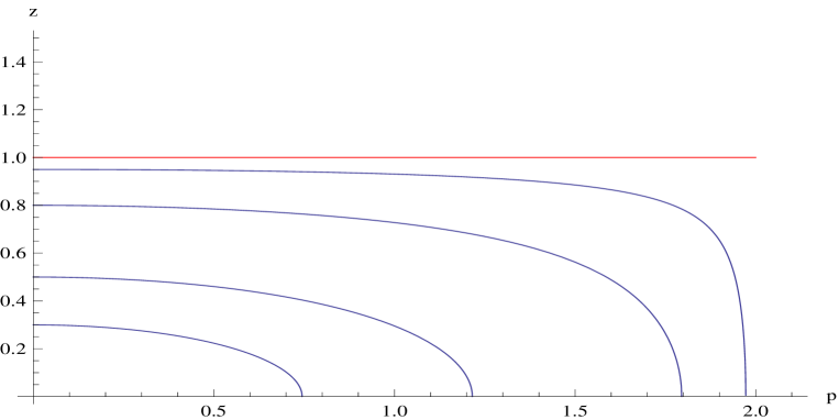
Fig. 4: Embedded solutions of $p(z)$ for $p_{0}=$ 0.74, 1.21, 1.79, and 1.97 from the below. Other parameters are set as $r_{0}$=1, $R$=1 and $a_{0}$=0.4. The horizontal line represents the domain wall.

In order to obtain the minimum of $S_{\rm area}$, we must solve the variational equation for $p(x)$ which is extended in the region $0<x<x_{0}$ of the bulk space. On the other hand, the information of the two boundary theories is divided by the domain wall as mentioned above. Then we will see the upperbound of $x_{0}$ at $x_{0}=1$. This point corresponds to $r=r_{0}$. This is actually assured by rewriting the above $S_{\rm area}$ as follows,

$${S_{\rm area}\over 4\pi} = \left({r_{0}\over R}a_{0}\right)^{3}\int dyf_{2}(y)\,$$ (59)

$$f_{2}(y) = \left({1+x^{2}\over x}\right)^{3}\sqrt{1+{b{(x^{\prime}p^{2}\gamma^{2})}^{2}\over(1+x^{2})^{2}}}\,$$ (60)

$$y = y(p)=\int^{p}dp{p^{2}\over(1-p^{2}/4)^{3}}\,,\quad x^{\prime}=\partial_{y}x\,.$$ (61)

These formula are very similar to the case of the Wilson loop calculation, where the embedded string configuration is obtained as a U-shaped one, and its bottom point is bounded at the minimum of the prefactor of the integrand. It corresponds here to

$$n_{Sphere}=\left({1+x^{2}\over x}\right)^{3}\,.$$ (62)

In fact we can see that $n_{Sphere}$ has a minimum at $x=1$. Then the embedded solution of the ball would be bounded in the region $0<x<1$, and this is also assured from the numerical calculation as shown in the Fig.4.

The analysis given above is obtained for $p(z)$ with various $p_{0}$, which is the value of $p$ at the UV limit $z=0$. The bottom point of $p(z)$ approaches to the value for $z=r_{0}$ (the horizontal line $x=1$). However, it does not never exceed this line. In other words, the quantum information of the theory on the other boundary does not affect on the EE calculation of the theory at $z=0$. This implies that there is no entanglement among the two theories on the opposite boundaries at $r=0(z=\infty)$ and $r=\infty(z=0)$.

Divergent term and central charge of the theory

While it is difficult to find an analytic solution of $p(z)$ in the present case, it is possible to see the divergent form of ${S_{\rm area}\over 4\pi}$ near the UV limit by using the approximate solution near the boundary. Before solving our present case, this point is shown firstly for the bulk AdS₅ case with Minkowski boundary metric. Through this analysis, we could obtain a knowledge related to the central charge of the theory. We write the AdS₅ metric as,

$$ds^{2}_{\rm AdS5}=\left({R\over z}\right)^{2}\left(\eta_{\mu\nu}dx^{\mu}dx^{\nu}+dz^{2}\right)\,.$$ (63)

In this case also, we use the same notation $p$ for the theree space radial coordinate as

$$ds^{2}_{(4)}=\eta_{\mu\nu}dx^{\mu}dx^{\nu}=-dt^{2}+dp^{2}+p^{2}d\Omega_{(2)}^{2}\,.$$ (64)

Then the 3D area of the embedded ball with radius $p_{0}$ is given as

$${S_{\rm area}\over{4\pi}}=R^{3}\int_{z_{\rm min}}^{z_{\rm max}}{dz\over z^{3}}p^{2}\sqrt{1+{p^{\prime}}^{2}}\,\,,$$ (65)

where $p^{\prime}=\partial p/\partial z$ and $\epsilon$ is the cutoff, namely $z>\epsilon$. In order to get the area of minimal surface, we should minimize $S_{\rm area}$. This requirement is achieved by the variational principle. The variational equation for $p(z)$ is solved in this case as

$$p=p_{0}+p_{2}z^{2}+p_{4}z^{4}+\cdots\,.$$ (66)

In the above, $p_{0}$ and $p_{4}$ are two arbitrary constants. This is the general solution. Simple power counting assures that only $p_{0}$ and $p_{2}$ are necessary to get divergent terms of $S_{\rm area}$. The value of $p_{2}$ is determined as

$$p_{2}=-{1\over{2p_{0}}}\,.$$ (67)

Using this solution, we can estimate the leading UV ($\epsilon\to 0$) divergent terms as

$${{S_{\rm area}}\over{4\pi}}={1\over 2}R^{3}\left[\left({{p_{0}^{2}}\over{\epsilon^{2}}}\right)+\log\left({{{\epsilon}\over{p_{0}}}}\right)\right]+{\rm finite~{}terms}\,,$$ (68)

where the parameter $p_{0}$, which characterize the present physical system, is introduced according to [35, 36].

The entanglement entropy is then expressed in the form used in [36] as follows

$$S_{EE}={{\gamma_{1}}\over 2}\cdot{{{\rm Area}(\partial A)}\over{4\pi\epsilon^{2}}}+\gamma_{2}\log\left(p_{0}\over{\epsilon}\right)+{\rm finite~{}terms}\,,$$ (69)

where ${{\rm Area}(\partial A)}$ denotes the area of the surface $A$, and $\gamma_{1}$ and $\gamma_{2}$ are numerical constants. In the present case, ${{\rm Area}(\partial A)}=4\pi p_{0}^{2}$ , then the coefficients $\gamma_{1}$ and $\gamma_{2}$ are obtained as

$${\gamma_{1}\over 2}={{2\pi R^{3}}\over{4G_{N}^{(5)}}}=N^{2}\,,\qquad\gamma_{2}={{2\pi R^{3}}\over{4G_{N}^{(5)}}}=N^{2}\,,$$ (70)

with the use of (52) and the relation $R^{4}=4\pi g_{s}{\alpha^{\prime}}^{2}N$. The result is compared to the corresponding divergent terms of our AdS₄ space model in the following.

Now we return to (56). In this case, the variational equation is solved by using the following expansion,

$$p=p_{0}+p_{2}x^{2}+p_{4L}x^{4}\log x+p_{4}x^{4}+\cdots\,.$$ (71)

The coefficients of this series expansion are determined by the two arbitrary constants, $p_{0}$ and $p_{4}$. The value of $p_{2}$ and $p_{4L}$ are determined as

$$p_{2}=-{{(1-(p_{0}^{2}/4)^{2})R^{4}}\over{2a_{0}^{2}p_{0}r_{0}^{2}}}\,.$$ (72)

and

$$p_{4L}=-\frac{\left(1-\left(\frac{p_{0}^{2}}{4}\right)^{2}\right)R^{8}\cos^{2}(\sqrt{\lambda_{0}}t)}{4a_{0}^{4}p_{0}r_{0}^{8}}.$$ (73)

This solution is not analytical in contrast to (66) due to the term $\log x$. However it is not important since only $p_{0}$ and $p_{2}$ contribute to the divergent terms of $S_{EE}$ as is mentioned above. The value of $p_{2}$ is determined as

$$p_{2}=-{{(1-(p_{0}^{2}/4)^{2})R^{4}}\over{2a_{0}^{2}p_{0}r_{0}^{2}}}\,.$$ (74)

With this solution, we obtain

$${{S_{\rm area}}\over{4\pi}}={1\over 2}R^{3}\left[\left({{k_{0}^{2}}\over{4\epsilon^{2}}}\sin^{2}(\sqrt{\lambda_{0}}t)\right)+(1+k_{0}^{2}\cos^{2}(\sqrt{\lambda_{0}}t))\log\left({{\epsilon}\over{p_{0}}}\right)\right]+{\rm finite~{}terms}\,,$$ (75)

where $k_{0}=p_{0}/(1-p_{0}^{2}/4)$. This result is also written in the form of (69) with the following coefficients $\gamma_{i}$,

$${\gamma_{1}\over 2} = {\lambda_{0}\over 4}N^{2}\,$$ (76)

$$\gamma_{2} = N^{2}\left(1+k_{0}^{2}\cos^{2}(\sqrt{\lambda_{0}}t)\right)\,.$$ (77)

where we used the following proper area in this case,

$${{\rm Area}(\partial A)}=4\pi k_{0}^{2}a_{0}(t)^{2}\,.$$ (78)

In this case $\gamma_{1}/2$ is slightly different by the factor ${\lambda_{0}/4}$ from the one of the AdS₅ case in (70). However, this difference can be removed by redefinition of the cut off parameter $\epsilon$. Then the remaining coefficient $N^{2}$ represents the freedom of the dual theory, and this is consistent with the previous result that the central charge of the dual theory has been given by $N^{2}$ through the calculation of the energy momentum tenser holographically (see the Appendix A) [16].

On the other hand, we find a definite difference in $\gamma_{2}$. This is understood from the fact that $\gamma_{2}$ depends on the curvatures in the 4D boundary and the extrinsic curvatures of the boundary $A$ in general [36]. When $t=(n+1/2)\pi/\sqrt{\lambda_{0}}$ ($n$ is an integer), $p_{4L}=0$ as seen from (73). In this case, $\gamma_{2}$ becomes the same with (70) and independent of $p_{0}$. Thus, there is a relation between $\gamma_{2}$ and $p_{4L}$. More precisely, $p_{4L}$ and the extra term in $\gamma_{2}$ both contain the facor $\cos^{2}(\sqrt{\lambda_{0}}t)$. While we are still considering about the physical interpretation of this relation, this is remained as an open question.

It would be an interesting problem to assure that our result could coincide with the one given from the side of the dual field theory, the SYM theory in the AdS₄ background, in order to see the validity of the gauge/gravity corresponding for our present model. This is remained here as an open question.

5 Summary and Discussions

In this paper, we have put forward an extended form of AdS₅/CFT₄ duality proposed in the previous paper [16], where AdS₅ is replaced by $\widetilde{AdS_{5}}$ whose boundary (in the ultraviolet side) is expressed by the FRW₄ space-time with finite 4D curvature. However the notation $\widetilde{AdS_{5}}$ might be missleading. It is because one might consider that, in order to get the solution $\widetilde{AdS_{5}}$, the equation of motion would be different from the one which leads to the ${AdS_{5}}$. Contrary to this expectation, $\widetilde{AdS_{5}}$ is a solution of the same 5D Einstein equation which leads to the typical ${AdS_{5}}$. Then the two solution are locally same with each other. On this point, we will discuss more in the next chance.

Two cases of the boundary geometry, AdS₄ and dS₄, are possible for this FRW₄ depending on the sign of the 4D cosmological constant $\Lambda_{4}$. The parameter $\Lambda_{4}$ can be introduced as an arbitrary constant in the process of solving the 5D Einstein equation with negative 5D cosmological constant $\Lambda$, which comes from five form field strength and is independent of $\Lambda_{4}$.

Here we point out a new holographic feature of the $\widetilde{AdS_{5}}$ with AdS₄ boundary. In this case, we observe second boundary in $\widetilde{AdS_{5}}$ at the opposite side of the fifth coordinate, namely at $r=0$ in addition to the one at $r=\infty$. This fact is in sharp contrast to the usual asymptotic AdS₅ case, in which the boundary appears only at $r=\infty$ and the point $r=0$ is usually set as a horizon.

This situation depends also on the other parameter $C$ in the general form of $\widetilde{AdS_{5}}$ given in (9)-(11), where $C$ denotes the dark radiation. While this term pushes the the domain wall to smaller $r$, we could find the boundary at $r=0$ for small value of $\tilde{c}_{0}$. However, the geometry of the boundary at $r=0$ is generally different from a simple AdS₄ which is realized at $r=\infty$. In the subsection 2.3, short discussion is given in the case of $C\neq 0$, in which it is pointed out that the metric of the IR boundary depends on the dark radiation or the SYM fields. On the other hand, at UV boundary the situation is different. Its geometry is not affected by the dark radiation. This point is interesting but we postpone to resolve this problem in the future.

Thus we restricted here to the case of $C=0$ and constant $\lambda$ in order to simplify the problem of two boundaries discussed in this article. In this case, we find that the metric of the UV boundary takes the form (20) and the one of IR boundary can be read from (17). They have the same form if $z$ was identified with $r$. Of course, they are different, but they are related as $z=r_{0}^{2}/r$ and the point $r=r_{0}$ has an important holographic meaning in the bulk. In fact, we find that this point corresponds to the domain wall.

As assured from the metric (17), we could observe that the 4D dual theory living at the boundary $r=0$ is also the SYM theory in the confinement phase. Furthermore, from the scaling behavior of the metric form of IR boundary (17), the limit of $r=0$ doesn’t correspond to the IR but to the UV limit of the corresponding 4D theory. Then there are two holographic screens in this case. This implies that the two field theories are described by a common gravity dual, $\widetilde{AdS_{5}}$ with AdS₄ boundary. We notice that we find one boundary at $r=\infty$ and a horizon in the infrared side at finite $r$ for another case of $\widetilde{AdS_{5}}$, which has dS₄ boundary.

The problem in the case of two boundaries is how the bulk manifold $\widetilde{AdS_{5}}$ would provide informations of the two field theories living on the different boundaries. Is it possible to get precise dynamical informations of two theories separately from the common bulk geometry? We could show that the answer is yes for this question interms of the presence of a sharp domain wall in the bulk. The gravity duals $\widetilde{AdS_{5}}$ for the two theories are separated by this wall.

The existence of the domain wall is assured by embedding the fundamental string, D7 brane and D5 brane in $\widetilde{AdS_{5}}$. These objects give us the information of the Wilson-Loop, quarks, meson spectrum and baryons of the dual SYM theory. We could find that the embedded regions of these objects are restricted to the either side of the bulk separated by the domain wall. In other words, these extended objects cannot be embedded across the domain wall. Then the property of the field theory in one boundary is given by the gavity of one-side bulk devided by the domain wall.

Another interesting embedding problem is found in the calculation of the entanglement entropy $S_{\rm EE}$. This is obtained by the minimal surface ${\rm Area}(\gamma_{A})$, which is defined as the minimum of the embedded surface whose boundary separates the fixed-time boundary space into two regions. In this calculation, we find the embedded surface never extend across the domain wall as other embedded stringy objects discussed above. This fact implies that the quantum fields in the theories of the two boundary don’t affect each other.

As for the entanglement entropy $S_{\rm EE}$ defined in either boundary. It diverges in general and written as (69). The two coefficients $\gamma_{1}$ and $\gamma_{2}$ of this expression reflect the freedom of the quantum fields of the theory and the geometry of the 4D space-time of the boundary respectively. The result, ${\gamma_{1}\over 2}=N^{2}$, is common to the one of the case of AdS₅ when we take the area of the sphere of the three space boundary by using the proper distance in the $\widetilde{AdS_{5}}$ case with AdS₄ boundary. On the other hand, $\gamma_{2}$ depends on the 4D curvatures and extrinsic curvatures on the 3D sphere. These quantities largely changes $\gamma_{2}$ of $\widetilde{AdS_{5}}$ from the one of AdS₅. Our result, (70), for $\gamma_{2}$ would be important to assure the curvature dependence of $S_{\rm EE}$ in curved space-time. We will discuss this point in the future work.

Finally we give the following two comments. First, the boundary of the AdS₅ is considered here as the point where double pole (as given by Witten in [1]) with respect to the fifth coordinate is observed. Two such points are found here at $r=0$ and $r=\infty$ for (A)dS₄ slice. Of course, another kinds of boundary can be considered as discussed in [37]. In [37], the authors have examined the bulk fields near a bulk singularity by supposing the existence of a new CFT there.

As for the boundary as a double pole point, the double boundaries are also observed in the black hole type solutions. In [38], the so called topological black hole solutions are discussed. While we don’t consider this type geometry, we can see that this case is similar to our solution of dS₄ slice since a horizon exists between the two boundaries in both cases.

Secondly, we should notice the following point. In [15], it is shown that our solutions used here can be rewritten to the form of the topological black hole solutions by a coordinate transformation. This is not surprising because both solutions are obtained from the same bulk Einstein equations which are derived from the action of Einstein-Hilbert and 5D cosmological constant as mentioned above. However, this transformation is performed in 5D by a kind of Rindler transformation, then the slice of the 4D space-time and the fifth coordinate are changed. As a result, the properties of the CFT in the sliced 4D space-time are also changed. This point is important and really assured by various holographic methods and quantities. So we think that the dual theory of the topological black hole is different from our presnt case given in this article. As mentioned in the first paragraph of this section, $\widetilde{AdS_{5}}$ is rewritten by ${AdS_{5}}$ through an appropriate coordinate transformation. However we should notice that we can see the properties of the CFT in 4D space-time, which is deformed from 4D Minkowski space-time, through $\widetilde{AdS_{5}}$.

Appendix

Appendix A $\langle T_{\mu\nu}\rangle$ of the dual theory at $r=\infty$

At first, we show 4D stress tensor of the boundary theory at $r=\infty$. Previously, it has already given, so we review it briefly. First we rewrite the 5d part of the metric (4) according to the Fefferman-Graham framework [25, 26, 27]. Then it is given as

$$ds^{2}_{(5)} = {1\over\rho}\left(-\bar{n}^{2}dt^{2}+\bar{A}^{2}a_{0}^{2}(t)\gamma^{2}(x)(dx^{i})^{2}\right)+{d\rho^{2}\over 4\rho^{2}}\,$$ (A.1)

$$= {1\over\rho}\hat{g}_{\mu\nu}dx^{\mu}dx^{\nu}+{d\rho^{2}\over 4\rho^{2}}\,,$$ (A.2)

where $\rho=1/r^{2}$, $R=1$ and

$$\bar{A} = \left(\left(1-{\lambda\over 4\mu^{2}}\left({\rho\over R^{2}}\right)\right)^{2}+\tilde{c}_{0}\left({\rho\over R^{2}}\right)^{2}\right)^{1/2}\,,$$ (A.3)

$$\bar{n} = {\left(1-{\lambda\over 4\mu^{2}}\left({\rho\over R^{2}}\right)\right)\left(1-{\lambda+\dot{\lambda}a_{0}/\dot{a}_{0}\over 4\mu^{2}}\left({\rho\over R^{2}}\right)\right)-\tilde{c}_{0}\left({\rho\over R^{2}}\right)^{2}\over\bar{A}}$$ (A.4)

In the next, $\hat{g}_{\mu\nu}$ is expanded as [26]

$$\hat{g}_{\mu\nu}={g}_{(0)\mu\nu}+{g}_{(2)\mu\nu}\rho+{\rho^{2}}\left({g}_{(4)\mu\nu}+{h}_{1(4)\mu\nu}\log\rho+{h}_{2(4)\mu\nu}(\log\rho)^{2}\right)+\cdots\,.$$ (A.5)

where

$${g}_{(0)\mu\nu}=({g}_{(0)00},~{}{g}_{(0)ij})=(-1,~{}a_{0}(t)^{2}\gamma_{i,j})\,,$$ (A.6)

and

$${g}_{(2)\mu\nu}={\lambda\over 2}\left(1+{{a_{0}\over\dot{a}_{0}}\dot{\lambda}\over\lambda},-~{}{g}_{(0)ij})\right)\,,$$ (A.7)

$${g}_{(4)\mu\nu}={\tilde{c}_{0}\over R^{4}}~{}(3,~{}{g}_{(0)ij})+{\lambda^{2}\over 16}~{}\left(-{(\lambda+{a_{0}\over\dot{a}_{0}}\dot{\lambda})^{2}\over\lambda^{2}},~{}{g}_{(0)ij}\right)\,.$$ (A.8)

Then by using the following formula [25],

$$\langle T_{\mu\nu}\rangle={4R^{3}\over 16\pi G_{N}}\left({g}_{(4)\mu\nu}-{1\over 8}{g}_{(0)\mu\nu}\left(({\rm Tr}g_{(2)})^{2}-{\rm Tr}g_{(2)}^{2}\right)-{1\over 2}\left({g}_{(2)}^{2}\right)_{\mu\nu}+{1\over 4}{g}_{(2)\mu\nu}{\rm Tr}g_{(2)}\right)\,,$$ (A.9)

we find

$$\langle T_{\mu\nu}\rangle=\langle\tilde{T}_{\mu\nu}^{(0)}\rangle+{4R^{3}\over 16\pi G_{N}^{(5)}}\left\{{3\lambda^{2}\over 16}\left(1,~{}\beta{g}_{(0)ij}\right)\right\}\,.$$ (A.10)

$$\langle\tilde{T}_{\mu\nu}^{(0)}\rangle={4R^{3}\over 16\pi G_{N}^{(5)}}{\tilde{c}_{0}\over R^{4}}(3,~{}{g}_{(0)ij})\,,\quad\beta=-\left(1+{2{a_{0}\over\dot{a}_{0}}\dot{\lambda}\over 3\lambda}\right)\,\,.$$ (A.11)

where $\langle\tilde{T}_{\mu\nu}^{(0)}\rangle$ comes from the conformal YM fields given in [16], so we find no anomaly for this component,

$$\langle\tilde{T}_{\mu}^{{(0)}\mu}\rangle=0\,.$$ (A.12)

The second term corresponds to the loop corrections of the YM fields in the curved space-time, and we find the conformal anomaly due to this term as

$$\langle T_{\mu}^{\mu}\rangle=-{3\lambda^{2}\left(1+{\dot{\lambda}\over 2\lambda}{a_{0}\over\dot{a}_{0}}\right)\over 8\pi^{2}}N^{2}\,,$$ (A.13)

where we used $G_{N}^{(5)}=8\pi^{3}{\alpha^{\prime}}^{4}g_{s}/R^{5}$ and $R^{4}=4\pi N{\alpha^{\prime}}^{2}g_{s}$.

The above anomaly (A.13) is obtained from the loop corrections of $\cal{N}=$ $4$ SYM theory in a space-time, $g_{(0)\mu\nu}$, which is given by (A.6). For this metric, the curvature squared terms responsible to the anomaly are given as

$$R^{\mu\nu\lambda\sigma}R_{\mu\nu\lambda\sigma} = 12\left(2\lambda^{2}+{\dot{\lambda}\lambda}{a_{0}\over\dot{a}_{0}}+\left(\dot{\lambda}{a_{0}\over 2\dot{a}_{0}}\right)^{2}\right)\,,$$ (A.14)

$$R^{\mu\nu}R_{\mu\nu} = 12\left(3\lambda^{2}+3{\dot{\lambda}\lambda}{a_{0}\over 2\dot{a}_{0}}+\left(\dot{\lambda}{a_{0}\over 2\dot{a}_{0}}\right)^{2}\right)\,,$$ (A.15)

$${1\over 3}R^{2} = 12\left(4\lambda^{2}+4{\dot{\lambda}\lambda}{a_{0}\over 2\dot{a}_{0}}+\left(\dot{\lambda}{a_{0}\over 2\dot{a}_{0}}\right)^{2}\right)\,.$$ (A.16)

In general, the conformal anomaly for $n_{s}$ scalars, $n_{f}$ Dirac fermions and $n_{v}$ vector fields is given as [29, 28]

$$\langle T_{\mu}^{\mu}\rangle=-{n_{s}+11n_{f}+62n_{v}\over 90\pi^{2}}E_{(4)}-{n_{s}+6n_{f}+12n_{v}\over 30\pi^{2}}I_{(4)}\,,$$ (A.17)

$$E_{(4)}={1\over 64}\left(R^{\mu\nu\lambda\sigma}R_{\mu\nu\lambda\sigma}-4R^{\mu\nu}R_{\mu\nu}+R^{2}\right)\,,$$ (A.18)

$$I_{(4)}=-{1\over 64}\left(R^{\mu\nu\lambda\sigma}R_{\mu\nu\lambda\sigma}-2R^{\mu\nu}R_{\mu\nu}+{1\over 3}R^{2}\right)\,,$$ (A.19)

where $\Box R$ has been abbreviated since it does not contribute here. For the $\cal{N}=$ $4$ SYM theory, the numbers of the fields are given by $N^{2}-1$ times the number of each fields, which are equivalent to $n_{s}=6$, $n_{f}=2$ and $n_{v}=1$. Then we find for large $N$,

$$\langle T_{\mu}^{\mu}\rangle={N^{2}\over 32\pi^{2}}\left(R^{\mu\nu}R_{\mu\nu}-{1\over 3}R^{2}\right)=-{3\lambda^{2}\left(1+{\dot{\lambda}\over 2\lambda}{a_{0}\over\dot{a}_{0}}\right)\over 8\pi^{2}}N^{2}\,.$$ (A.20)

This result (A.20) is precisely equivalent to the above holographic one (A.13). Thus we could see that the holographic analysis could give correct results for the energy momentum tensor even if the metric is time dependent as shown previously in [16].

Appendix B $\langle T_{\mu\nu}^{\rm IR}\rangle$ of the dual theory at $r=0$

In the IR side, we get $\langle T_{\mu\nu}^{\rm IR}\rangle$ by the parallel method. By using the above formula (A.9), we find

$$\langle T_{\mu\nu}^{\rm IR}\rangle = {4R^{3}\over 16\pi G_{N}^{(5)}}~{}\left(\hat{g}_{(0)00}~{}t_{00},~{}\hat{g}_{(0)ij}~{}t_{11}\right)\,$$ (B.1)

$$t_{00} = -{3r_{0}^{8}\over{r^{*}}^{4}+\tilde{c}_{0}}\,,\quad t_{11}=-r_{0}^{8}{2{r^{*}}^{4}+({r^{*}}{r^{*}}_{1})^{2}+\tilde{c}_{0}\over({r^{*}}^{4}+\tilde{c}_{0})(({r^{*}}{r^{*}}_{1})^{2}-\tilde{c}_{0})}\,,$$ (B.2)

This result should be interpreted as the VEV of the energy momentum tensor of the SYM theory living in the space-time $\hat{g}_{(0)\mu\nu}$ given by (23). In the present case, however, both the metric $\hat{g}_{(0)\mu\nu}$ and the $\langle T_{\mu\nu}\rangle$ are different from the one given at the boundary $r\to\infty$. Then we must check how the two theories on the each boundary are different. We perform this for the following three cases.

One expect that the central charges on each boundaries would be different from each other since the renormalization group flow would be different. The answer for this issue is given by observing the trace anomaly, which is found from the above $\langle T_{\mu\nu}\rangle$ as follows,

$$\langle T^{\mu}_{\mu}\rangle = {4R^{3}\over 16\pi G_{N}^{(5)}}~{}\left(t_{00}+3t_{11}\right)\,$$ (B.3)

$$= -{N^{2}\over 2\pi^{2}}{6r_{0}^{8}{r^{*}}^{2}(({r^{*}}^{2}+{r^{*}}_{1})^{2})\over({r^{*}}^{4}+\tilde{c}_{0})(({r^{*}}{r^{*}}_{1})^{2}-\tilde{c}_{0})}\,,$$ (B.4)

where we used $G_{N}^{(5)}=8\pi^{3}{\alpha^{\prime}}^{4}g_{s}/R^{5}$ and $R^{4}=4\pi N{\alpha^{\prime}}^{2}g_{s}$. This is rewritten by using the relation

$$W_{IR} = \left(R^{\mu\nu}R_{\mu\nu}-{1\over 3}R^{2}\right)\,$$ (B.5)

$$= -16{6r_{0}^{8}{r^{*}}^{2}({r^{*}}^{2}+{r^{*}}_{1}^{2})\over({r^{*}}^{4}+\tilde{c}_{0})(({r^{*}}{r^{*}}_{1})^{2}-\tilde{c}_{0})}\,,$$ (B.6)

we obtain

$$\langle T^{\mu}_{\mu}\rangle={N^{2}\over 32\pi^{2}}W_{IR}\,.$$ (B.7)

References

- [1] J. M. Maldacena, Adv. Theor. Math. Phys. 2, 231 (1998) [hep-th/9711200]. S. S. Gubser, I. R. Klebanov and A. M. Polyakov, Phys. Lett. B 428, 105 (1998) [hep-th/9802109]. E. Witten, Adv. Theor. Math. Phys. 2, 253 (1998) [hep-th/9802150]. A.M. Polyakov, Int. J. Mod. Phys. A14 (1999) 645, (hep-th/9809057).
- [2] A. Karch and E. Katz, JHEP 0206, 043(2003) [hep-th/0205236].
- [3] M. Kruczenski, D. Mateos, R.C. Myers and D.J. Winters, JHEP 0307, 049(2003) [hep-th/0304032].
- [4] M. Kruczenski, D. Mateos, R.C. Myers and D.J. Winters, [hep-th/0311270].
- [5] J. Babington, J. Erdmenger, N. Evans, Z. Guralnik and I. Kirsch, hep-th/0306018.
- [6] N. Evans, and J.P. Shock, hep-th/0403279.
- [7] T. Sakai and J. Sonnenshein, [hep-th/0305049].
- [8] C. Nunez, A. Paredes and A.V. Ramallo, JHEP 0312, 024(2003) [hep-th/0311201].
- [9] K. Ghoroku and M. Yahiro, Phys. Lett. B 604, 235(2004), [hep-th/0408040].
- [10] R. Casero, C. Nunez and A. Paredes, Phys.Rev. D73 (2006) 086005.
- [11] T. Hirayama, JHEP 0606, 013(2006) [hep-th/0602258].
- [12] K. Ghoroku M. Ishihara and A. Nakamura, Phys. Rev. D74 124020 (2006) .
- [13] K. Ghoroku M. Ishihara and A. Nakamura, Phys. Rev. D75 046005 (2007) .
- [14] J. Erdmenger, K. Ghoroku, R. Meyer, ”Holographic (De)confinement Transitions in Cosmological Backgrounds ”, Phys.Rev.D84:026004,2011, [arXiv:1105.1776 (hep-th)]
- [15] J. Erdmenger, K. Ghoroku, R. Meyer, Ioannis Papadimitriou, ”Holographic Cosmological Backgrounds, Wilson Loop (De)confinement and Dilaton Singularities” [arXiv:1205.0677 (hep-th)]
- [16] K. Ghoroku and A. Nakamura, Phys. Rev. D87 063507 (2013) . ”Holographic Fridmann equation and N=4 supersymmetric Yang-Mills theory” [arXiv:1212.2304 (hep-th)]
- [17] S. Gubser, [hep-th/9902155]
- [18] P. Binetruy, C. Deffayet, U. Ellwanger and D. Langlois, Phys.Lett. B477 (2000) 285-291,[hep-th/9910219]
- [19] D. Langlois, hep-th/0005025, 0306281
- [20] A. Kehagias and K. Sfetsos, Phys. Lett. B 456, 22(1999) [hep-th/9903109].
- [21] H. Liu and A.A. Tseytlin [hep-th/9903091].
- [22] G. W. Gibbons, M. B. Green and M. J. Perry, Phys.Lett. B370 (1996) 37-44, [hep-th/9511080].
- [23] S.J. Avis, C.J. Isham and D. Storey, Phys. Rev. D 18, 3565 (1978).
- [24] K. Skenderis, Class. Quant. Grav. 19, 5849 (2002) [hep-th/0209067].
- [25] S. de Haro, S. N. Solodukhin and K. Skenderis, Commun. Math. Phys. 217, 595 (2001) [hep-th/0002230].
- [26] Massimo Bianchi, Daniel Z. Freedman, Kostas Skenderis, Nucl.Phys. B631 (2002) 159-194, [hep-th/0112119].
- [27] C. Fefferman and C. Robin Graham, ‘Conformal Invariants’, in Elie Cartan et les Mathématiques d’aujourd’hui (Astérisque, 1985) 95.
- [28] M.J. Duff, Class.Quant.Grav. 11 (1994) 1387-1404,[hep-th/9308075]
- [29] N.D. Birrell and P.C.W. Davies, ”Quantum fields in curved space” 1982, Cambridge Univ. Press.
- [30] E. Witten, “Baryons and Branes in Anti de Sitter Space,” J. High Energy Phys. 07 (1998) 006, hep-th/9805112.
- [31] Y. Imamura, “Supersymmetries and BPS Configurations on Anti-de Sitter Space,” Nucl. Phys. B537 (1999) 184, hep-th/9807179.
- [32] C. G. Callan, A. Güijosa, and K. Savvidy, “Baryons and String Creation from the Fivebrane Worldvolume Action,” hep-th/9810092.
- [33] C. G. Callan, A. Güijosa, K. G. Savvidy and O. Tafjord, “Baryons and flux tubes in confining gauge theories from brane actions,” Nucl. Phys. B 555 (1999) 183 [arXiv:hep-th/9902197].
-
[34]
K. Ghoroku, M. Ishihara,
“Baryons with D5 Brane Vertex and -quarks states,”
Phys. Rev. D 77, 086003 (2008)
[arXiv:hep-th/0801.4216].
K. Ghoroku, M. Ishihara, A. Nakamura and F. Toyoda, “Multi-quark baryon and color screening at finite temperature,” Phys. Rev. D 79, 066009 (2009) [arXiv:hep-th/0806.0195]. -
[35]
S. Ryu, T. Takayanagi,
“Holographic derivation of entanglement entropy from AdS/CFT ,”
Phys. Rev. Lett 96, 181602 (2006)
[arXiv:hep-th/0603001].
-
[36]
S. Ryu, T. Takayanagi,
“Holographic derivation of entanglement entropy from AdS/CFT ,”
J. High Energy Phys. 08 (2006) 045,
[arXiv:hep-th/0605073].
-
[37]
Shin’ichi Nojiri, Sergei D. Odintsov,
”Two-Boundaries AdS/CFT Correspondence in Dilatonic Gravity”, Phys.Lett.B449:39-47,1999,
[arXiv:hep-th/9812017].
-
[38]
Roberto Emparan, ”AdS/CFT Duals of Topological Black Holes and the Entropy of Zero-Energy States”, JHEP 9906 (1999) 036, [arXiv:hep-th/906040].