High Dimensional Stochastic Regression with Latent Factors, Endogeneity and Nonlinearity

Abstract

We consider a multivariate time series model which represents a high dimensional vector process as a sum of three terms: a linear regression of some observed regressors, a linear combination of some latent and serially correlated factors, and a vector white noise. We investigate the inference without imposing stationary conditions on the target multivariate time series, the regressors and the underlying factors. Furthermore we deal with the the endogeneity that there exist correlations between the observed regressors and the unobserved factors. We also consider the model with nonlinear regression term which can be approximated by a linear regression function with a large number of regressors. The convergence rates for the estimators of regression coefficients, the number of factors, factor loading space and factors are established under the settings when the dimension of time series and the number of regressors may both tend to infinity together with the sample size. The proposed method is illustrated with both simulated and real data examples.

Keywords: $\alpha$-mixing, dimension reduction, instrument variables, nonstationarity, time series

JEL classification: C13; C32; C38.

1 Introduction

In this modern information age, the availability of large or vast time series data bring the opportunities with challenges to time series analysts. The demand of modelling and forecasting high-dimensional time series arises from various practical problems such as panel study of economic, social and natural (such as weather) phenomena, financial market analysis, communications engineering. On the other hand, modelling multiple time series even with moderately large dimensions is always a challenge. Although a substantial proportion of the methods and the theory for univariate autoregressive and moving average (ARMA) models has found the multivariate counterparts, the usefulness of unregularized multiple ARMA models suffers from the overparametrization and the lack of the identification (Lütkepohl, 2006). Various methods have been developed to reduce the number of parameters and to eliminate the non-identification issues. For example, Tiao and Tsay (1989) proposed to represent a multiple series in terms of several scalar component models based on canonical correlation analysis, Jakeman et al. (1980) adopted a two stage regression strategy based on instrumental variables to avoid using moving average explicitly. Another popular approach is to represent multiple time series in terms of a few factors defined in various ways; see, among others, Stock and Watson (2005), Bai and Ng (2002), Forni et al. (2005), Lam et al. (2011), and Lam and Yao (2012). Davis et al. (2012) proposed a vector autoregressive (VAR) model with sparse coefficient matrices based on partial spectral coherence. LASSO regularization has also been applied in VAR modelling; see, for example, Shojaie and Michailidis (2010) and Song and Bickel (2011).

This paper can be viewed as a further development of Lam et al. (2011) and Lam and Yao (2012) which express a high-dimensional vector time series as a linear transformation of a low-dimensional latent factor process plus a vector white noise. We extend their methodology and explore three new features. We only deal with the cases when the dimension is large in relation to the sample size. Hence all asymptotic theory is developed when both the sample size and the dimension of time series tend to infinity together.

Firstly, we add a regression term to the factor model. This is a useful addition as in many applications there exist some known factors which are among the driving forces for the dynamics of most the component series. For example, temperature is an important factor in forecasting household electricity consumptions. The price of a product plays a key role in its sales over different regions. The capital asset pricing model (CAPM) theory implies that the market index is a common factor for pricing different assets. When the regressor and the latent factor are uncorrelated, we estimate the regression coefficients first by the least squares method. We then estimate the number of factors and the factor loading space based on the residuals resulted from the regression estimation. We show that the latter is asymptotically adaptive to the unknown regression coefficients in the sense that the convergence rates for estimating the factor loading space and the factor process are the same as if the regression coefficients were known. We also consider the models with endogeneity in the sense that there exist correlations between the regressors and the latent factors. We show that the factor loading space can still be identified and estimated consistently in the presence of the endogeneity. However relevant instrumental variables need to be employed if the ‘original’ regression coefficients have to be estimated consistently. The exploration in this direction has some overlap with Pesaran and Tosetti (2011), although the models, the inference methods and the asymptotic results in the two papers are different.

Our second contribution lies in the fact that we do not impose stationarity conditions on the regressors and the latent factor process throughout the paper. This enlarges the potential application substantially, as many important factors in practical problems (such as temperature, calendar effects) are not stationary. Different from the method of Pan and Yao (2008) which can also handle nonstationary factors but is computationally expensive, our approach is a direct extension of Lam et al. (2011) and Lam and Yao (2012) and, hence, is applicable to the cases when the dimensions of time series is in the order of thousands with an ordinary personal computer.

Finally, we focus on the factor models with a nonlinear regression term. By expressing the nonlinear regression function as a linear combination of some base functions, we turn the problem into the model with a large number of linear regressors. Now the asymptotic theory is established when the sample size, the dimension of time series and the number of regressors go to infinity together.

The rest of the paper is organized as follows. Section 2 deals with linear regression models with latent factors but without endogeneity. The models with the endogeneity are handled in Section 3. Section 4 investigates the models with nonlinear regression term. Simulation results are reported in Section 5. Illustration with some stock prices included in S&P500 is presented in Section 6. All the technical proofs are relegated to the Appendix.

2 Regression with latent factors

2.1 Models

Consider the regression model

$${\bf y}_{t}={\bf D}{\bf z}_{t}+{\bf A}{\bf x}_{t}+\mbox{\boldmath$\varepsilon$}_{t},$$ (1)

where $\mbox{\bf y}_{t}$ and ${\bf z}_{t}$ are, respectively, observable $p\times 1$ and $m\times 1$ time series, $\mbox{\bf x}_{t}$ is an $r\times 1$ latent factor process, $\mbox{\boldmath$\varepsilon$}_{t}\sim\textrm{WN}(0,{\bf\Sigma}_{\varepsilon})$ is a white noise with zero mean and covariance matrix ${\bf\Sigma}_{\varepsilon}$ and $\mbox{\boldmath$\varepsilon$}_{t}$ is uncorrelated with $(\mbox{\bf z}_{t},\mbox{\bf x}_{t})$, ${\bf D}$ is an unknown regression coefficient matrix, and ${\bf A}$ is an unknown factor loading matrix. The number of the latent factors $r$ is an unknown (fixed) constant. With the observations $\{(\mbox{\bf y}_{t},\mbox{\bf z}_{t}):\;t=1,\ldots,T\}$, the goal is to estimate ${\bf D},\;{\bf A}$ and $r$, and to recover the factor process $\mbox{\bf x}_{t}$, when $p$ is large in relation to the sample size $T$. As our inference will be based on the serial dependence of each and across $\mbox{\bf y}_{t},\mbox{\bf z}_{t}$ and $\mbox{\bf x}_{t}$, we assume $E({\bf z}_{t})={\bf 0}$ and $E({\bf x}_{t})={\bf 0}$ for simplicity.

In this section, we consider the simple case when $\mbox{\bf z}_{t}$ and $\mbox{\bf x}_{t}$ are uncorrelated. This condition ensures that the coefficient matrix D in (1) is identifiable. However the factor loading matrix A and the factor $\mbox{\bf x}_{t}$ are not uniquely determined by (1), as we may replace $({\bf A},{\bf x}_{t})$ by $({\bf A}{\bf H},{\bf H}^{-1}{\bf x}_{t})$ for any invertible matrix ${\bf H}$. Nevertheless the linear space spanned by the columns of ${\bf A}$, denoted by $\mathcal{M}({\bf A})$, is uniquely defined. $\mathcal{M}({\bf A})$ is called the factor loading space. Hence there is no loss of the generality in assuming that A is a half orthogonal matrix in the sense that $\mbox{\bf A}^{\mathrm{\scriptscriptstyle T}}\mbox{\bf A}=\mbox{\bf I}_{r}$. In this paper, we always adhere with this assumption. Once we have specified a particular A, $\mbox{\bf x}_{t}$ is uniquely defined accordingly. On the other hand, when $\textrm{cov}(\mbox{\bf z}_{t},\mbox{\bf x}_{t})\neq{\bf 0}$, the endogeneity makes D unidentifiable, which will be dealt with in Section 3 below.

2.2 Estimation

Formally the estimation for D may be treated as a standard least squares problem, since

$${\bf y}_{t}={\bf D}{\bf z}_{t}+\mbox{\boldmath$\eta$}_{t},\qquad\mbox{\boldmath$\eta$}_{t}=\mbox{\bf A}\mbox{\bf x}_{t}+\mbox{\boldmath$\varepsilon$}_{t},$$ (2)

and cov$(\mbox{\bf z}_{t},\mbox{\boldmath$\eta$}_{t})={\bf 0}$; see (1). Write ${\bf D}=({\bf d}_{1},\ldots,{\bf d}_{p})^{\mathrm{\scriptscriptstyle T}}$. The least squares estimator for ${\bf D}$ can be expressed as

$$\widehat{{\bf D}}=(\widehat{{\bf d}}_{1},\ldots,\widehat{{\bf d}}_{p})^{\mathrm{\scriptscriptstyle T}},\qquad\widehat{{\bf d}}_{i}=\bigg{(}\frac{1}{T}\sum_{t=1}^{T}{\bf z}_{t}{\bf z}_{t}^{\mathrm{\scriptscriptstyle T}}\bigg{)}^{-1}\bigg{(}\frac{1}{T}\sum_{t=1}^{T}y_{i,t}\,{\bf z}_{t}\bigg{)},$$ (3)

where $y_{i,t}$ is the $i$th component of $\mbox{\bf y}_{t}$.

The estimation for $\mathcal{M}(\mbox{\bf A})$ is based on the residuals $\widehat{}\mbox{\boldmath$\eta$}_{t}=\mbox{\bf y}_{t}-\widehat{}\mbox{\bf D}\mbox{\bf z}_{t}$, using the same idea as Lam et al. (2011) and Lam and Yao (2012), though we do not assume that the processes concerned are stationary. To this end, we introduce some notation first. Let

$$\mbox{\boldmath$\Sigma$}_{x}(k)=\frac{1}{T-k}\sum_{t=1}^{T-k}\textrm{cov}({\bf x}_{t+k},{\bf x}_{t}),\qquad\mbox{\boldmath$\Sigma$}_{x\varepsilon}(k)=\frac{1}{T-k}\sum_{t=1}^{T-k}\textrm{cov}({\bf x}_{t+k},\mbox{\boldmath$\varepsilon$}_{t}),$$

$$\mbox{\boldmath$\Sigma$}_{\eta}(k)=\frac{1}{T-k}\sum_{t=1}^{T-k}\textrm{cov}(\mbox{\boldmath$\eta$}_{t+k},\mbox{\boldmath$\eta$}_{t}).$$

When, for example, $\mbox{\bf x}_{t}$ is stationary, $\mbox{\boldmath$\Sigma$}_{x}(k)$ is the autocovariance matrix of $\mbox{\bf x}_{t}$ at lag $k$. It follows from the second equation in (2) that for any $k\neq 0$,

$$\mbox{\boldmath$\Sigma$}_{\eta}(k)={\bf A}\mbox{\boldmath$\Sigma$}_{x}(k){\bf A}^{\mathrm{\scriptscriptstyle T}}+{\bf A}\mbox{\boldmath$\Sigma$}_{x\varepsilon}(k).$$ (4)

For a prescribed fixed positive integer $\bar{k}$, define

$${\bf M}=\sum_{k=1}^{\bar{k}}\mbox{\boldmath$\Sigma$}_{\eta}(k)\mbox{\boldmath$\Sigma$}_{\eta}(k)^{\mathrm{\scriptscriptstyle T}}.$$ (5)

We assume rank$(\mbox{\bf M})=r$. This is reasonable as it effectively assumes that the latent factor process $\mbox{\bf x}_{t}$ is genuinely $r$-dimensional. Since M is implicitly sandwiched by A and $\mbox{\bf A}^{\mathrm{\scriptscriptstyle T}}$, $\mbox{\bf M}\mbox{\bf b}={\bf 0}$ for any $\mbox{\bf b}\perp\mathcal{M}(\mbox{\bf A})$. Thus we may take the eigenvectors of M corresponding to non-zero eigenvalues as the columns of A, as the choice of A is almost arbitrary as long as $\mathcal{M}(\mbox{\bf A})$ does not change. Let $\mbox{\bf A}=(\mbox{\bf a}_{1},\ldots,\mbox{\bf a}_{r})$, where $\mbox{\bf a}_{1},\ldots,\mbox{\bf a}_{r}$ be the $r$ orthonormal eigenvectors of M corresponding to the $r$ largest eigenvalues $\lambda_{1}\geq\cdots\geq\lambda_{r}>0$. Then A is a half orthogonal matrix in the sense that $\mbox{\bf A}^{\mathrm{\scriptscriptstyle T}}\mbox{\bf A}=\mbox{\bf I}_{r}$. In the sequel, we always use A defined this way. When the $r$ non-zero eigenvalues of M are distinct, A is unique if we ignore the trivial replacements of $\mbox{\bf a}_{j}$ by $-\mbox{\bf a}_{j}$.

Let $\widehat{}\mbox{\boldmath$\eta$}_{t}=\mbox{\bf y}_{t}-\widehat{}\mbox{\bf D}\mbox{\bf z}_{t}$ and

$$\widehat{}\mbox{\boldmath$\Sigma$}_{\eta}(k)={1\over T-k}\sum_{t=1}^{T-k}(\widehat{}\mbox{\boldmath$\eta$}_{t+k}-\bar{\mbox{\boldmath$\eta$}})(\widehat{}\mbox{\boldmath$\eta$}_{t}-\bar{\mbox{\boldmath$\eta$}})^{\mathrm{\scriptscriptstyle T}},\qquad\bar{\mbox{\boldmath$\eta$}}=\frac{1}{T}\sum_{t=1}^{T}\widehat{}\mbox{\boldmath$\eta$}_{t}.$$

The above discussion leads to a natural estimator of A denoted by $\widehat{}\mbox{\bf A}\equiv(\widehat{}\mbox{\bf a}_{1},\ldots,\widehat{}\mbox{\bf a}_{r})$. Here $\widehat{}\mbox{\bf a}_{1},\ldots,\widehat{}\mbox{\bf a}_{r}$ are the orthonormal eigenvectors of $\widehat{}\mbox{\bf M}$ corresponding to the $r$ largest eigenvalues $\widehat{\lambda}_{1}\geq\cdots\geq\widehat{\lambda}_{r}$, where

$$\widehat{}\mbox{\bf M}=\sum_{k=1}^{\bar{k}}\widehat{}\mbox{\boldmath$\Sigma$}_{\eta}(k)\widehat{}\mbox{\boldmath$\Sigma$}_{\eta}(k)^{\mathrm{\scriptscriptstyle T}}.$$ (6)

Since $\widehat{}\mbox{\bf A}$ is a half orthogonal matrix, we may extract the factor process by $\widehat{}\mbox{\bf x}_{t}=\widehat{\bf A}^{\mathrm{\scriptscriptstyle T}}(\mbox{\bf y}_{t}-\widehat{}\mbox{\bf D}\mbox{\bf z}_{t})$; see (2).

All the arguments above are based on a known $r$ which is actually unknown in practice. The determination of $r$ is a key step in our inference. In practice we may estimate it by the ratio estimator

$$\widehat{r}=\arg\min\bigg{\{}\frac{\widehat{\lambda}_{j+1}}{\widehat{\lambda}_{j}}:1\leq j\leq R\bigg{\}},$$ (7)

where $\widehat{\lambda}_{1}\geq\cdots\geq\widehat{\lambda}_{p}$ are the eigenvalues of $\widehat{}\mbox{\bf M}$, and $R$ is a constant which may be taken as $R=p/2$; see Lam and Yao (2012) for further discussion on this estimation method.

2.3 Asymptotic properties

We present the asymptotic theory for the estimation methods described in Section 2.2 above when $T,\;p\to\infty$ while $r$ is fixed. We also assume $m$ fixed now; see Section 4 below for the results when $m\to\infty$ as well. We do not impose stationarity conditions on $\mbox{\bf y}_{t},\mbox{\bf z}_{t}$ and $\mbox{\bf x}_{t}$. Instead we assume that they are mixing processes; see Condition 2.1 below. Hence our results in the special case when $\mbox{\bf z}_{t}\equiv\bf 0$ extend those in Lam et al. (2011) and Lam and Yao (2012) to nonstationary cases. Pan and Yao (2008) dealt with a different method for nonstationary factor models.

We introduce some notation first. For any matrix H, we denote by $\|\mbox{\bf H}\|_{F}=\{{\rm tr}(\mbox{\bf H}^{\mathrm{\scriptscriptstyle T}}\mbox{\bf H})\}^{1/2}$ the Frobenius norm of H, and by $\|\mbox{\bf H}\|_{2}=\{\lambda_{\max}(\mbox{\bf H}^{\mathrm{\scriptscriptstyle T}}\mbox{\bf H})\}^{1/2}$ the $L_{2}$-norm, where tr$(\cdot)$ and $\lambda_{\max}(\cdot)$ denote, respectively, the trace and the maximum eigenvalue of a square matrix. We also denote by $\|\mbox{\bf H}\|_{\min}$ the square-root of the minimum nonzero eigenvalue of $\mbox{\bf H}^{\mathrm{\scriptscriptstyle T}}\mbox{\bf H}$. Note that when $\mbox{\bf H}=\mbox{\bf h}$ is a vector, $\|\mbox{\bf h}\|_{F}=\|\mbox{\bf h}\|_{2}=\|\mbox{\bf h}\|_{\min}=(\mbox{\bf h}^{\mathrm{\scriptscriptstyle T}}\mbox{\bf h})^{1/2}$, i.e. the conventional Euclidean norm for vector h.

Condition 2.1.

The process $\{(\mbox{\bf y}_{t},\mbox{\bf z}_{t},\mbox{\bf x}_{t})\}$ is $\alpha$-mixing with the mixing coefficients satisfying the condition $\sum_{k=1}^{\infty}\alpha(k)^{1-2/\gamma}<\infty$ for some $\gamma>2$, where

$$\alpha(k)=\sup_{i}\sup_{A\in\mathcal{F}_{-\infty}^{i},\;B\in\mathcal{F}_{i+k}^{\infty}}\big{|}P(A\cap B)-P(A)P(B)\big{|},$$

and $\mathcal{F}_{i}^{j}$ is the $\sigma$-field generated by $\{(\mbox{\bf y}_{t},\mbox{\bf z}_{t},\mbox{\bf x}_{t}):\;i\leq t\leq j\}$.

Condition 2.2.

For any $i=1,\ldots,m$, $j=1,\ldots,p$ and $t$, $E(|z_{i,t}|^{2\gamma})\leq C_{1}$, $E(|\zeta_{j,t}|^{2\gamma})\leq C_{1}$ and $E(|\varepsilon_{j,t}|^{2\gamma})\leq C_{1}$, where $C_{1}>0$ is a constant, $\gamma$ is given in Condition 2.1, and $z_{i,t}$ is the $i$th element of ${\bf z}_{t}$, $\zeta_{j,t}$ and $\varepsilon_{j,t}$ are the $j$th element of, respectively, $\mbox{\bf A}\mbox{\bf x}_{t}$ and $\mbox{\boldmath$\varepsilon$}_{t}$.

Condition 2.3.

There exists a constant $C_{2}>0$ such that $\lambda_{\textrm{min}}\{E({\bf z}_{t}{\bf z}_{t}^{\mathrm{\scriptscriptstyle T}})\}>C_{2}$ for all $t$.

Condition $E(|\zeta_{j,t}|^{2\gamma})\leq C_{1}$ in Condition 2.2 can be guaranteed by some suitable conditions on each $x_{i,t}$, as ${\bf A}$ is a half orthogonal matrix. For example, it holds if $\max_{i,t}E(|x_{i,t}|^{2\gamma})<\infty$. Proposition 2.1 below establishes the convergence rate of the estimator for the $p\times m$ coefficient matrix D. Since $p\to\infty$ together with the sample size $T$, the convergence rate depends on $p$. Especially when $p/T\to 0$, the least squares estimator $\widehat{}\mbox{\bf D}$ is a consistent estimator for D. This condition can be relaxed if we impose some sparse condition on D, and then apply appropriate thresholding on $\widehat{}\mbox{\bf D}$. We do not pursue this further here. When $p$ is fixed, the convergence rate is $T^{1/2}$ which is the optimal rate for the regression with the dimension fixed.

Proposition 2.1.

Let Conditions 2.1-2.3 hold. As $T\to\infty$ and $p\to\infty$, it holds that

$$\|\widehat{{\bf D}}-{\bf D}\|_{F}=O_{p}\big{(}p^{1/2}T^{-1/2}\big{)}.$$

To state the results for estimating factor loadings, we introduce more conditions.

Condition 2.4.

There exist positive constants $C_{i}~{}(i=3,4)$ and $\delta\in[0,1]$ such that $C_{3}p^{1-\delta}\leq\|\mbox{\boldmath$\Sigma$}_{x}(k)\|_{\min}\leq\|\mbox{\boldmath$\Sigma$}_{x}(k)\|_{2}\leq C_{4}p^{1-\delta}$ for all $k=1,\ldots,\bar{k}$.

Condition 2.5.

Matrix M admits $r$ distinct positive eigenvalues $\lambda_{1}>\cdots>\lambda_{r}>0$.

The constant $\delta$ in Condition 2.4 controls the strength of the factors. When $\delta=0$, the factors are strong. When $\delta>0$, the factors are weak. In fact the value of $\delta$ reflects the sparse level of the factor loading matrix A, and a certain degree of sparsity is present when $\delta>0$. Therefore not all components of $\mbox{\bf y}_{t}-\mbox{\bf D}{\bf z}_{t}$ carry the information for all factor components. This causes difficulties in recovering the factor process. This argument will be verified in Theorem 2.2. See also Remark 1 in Lam and Yao (2012). Condition 2.5 implies that A defined as in Section 2.2 above is unique. This simplifies the presentation significantly, as Theorem 2.1 below can present the convergence rates of the estimator for A directly. Without condition 2.5, the same convergence rates can be obtained for the estimation of the linear space $\mathcal{M}(\widehat{\mbox{\bf A}})$; see (9) below. Let

$$\kappa_{1}=\min_{1\leq k\leq\bar{k}}\|\mbox{\boldmath$\Sigma$}_{x\varepsilon}(k)\|_{\min}~{}~{}\textrm{and}~{}~{}\kappa_{2}=\max_{1\leq k\leq\bar{k}}\|\mbox{\boldmath$\Sigma$}_{x\varepsilon}(k)\|_{2}.$$

Note that both $\kappa_{1}$ and $\kappa_{2}$ may diverge as $p\to\infty$.

Theorem 2.1.

Let Conditions 2.1-2.5 hold. Suppose that $r$ is known and fixed, then

$$\|\widehat{{\bf A}}-{\bf A}\|_{2}=~{}\left\{\begin{array}[]{ll}O_{p}(p^{\delta}T^{-1/2}),&{\rm if\;}\kappa_{2}=o(p^{1-\delta}){\rm\;\;and\;\;}p^{2\delta}T^{-1}=o(1);\\[4.30554pt] O_{p}(\kappa_{1}^{-2}\kappa_{2}pT^{-1/2}),&{\rm if\;}p^{1-\delta}=o(\kappa_{1}){\rm\;\;and\;\;}\kappa_{1}^{-2}\kappa_{2}pT^{-1/2}=o(1).\end{array}\right.$$

The convergence rates in Theorem 2.1 above are exactly the same as Theorem 1 of Lam et al. (2011) which deals with a pure factor model, i.e. model (2) with $\mbox{\bf z}_{t}\equiv\bf 0$. In this sense, the estimator $\widehat{}\mbox{\bf A}$ is asymptotically adaptive to unknown D.

Theorem 2.2.

Let Conditions 2.1-2.5 hold, and $r$ be known and fixed. If $\|\mbox{\boldmath$\Sigma$}_{\varepsilon}\|_{2}$ is bounded as $p\to\infty$, then

$$p^{-1/2}\|\widehat{{\bf A}}\widehat{{\bf x}}_{t}-{\bf A}{\bf x}_{t}\|_{2}=O_{p}(\|\widehat{{\bf A}}-{\bf A}\|_{2}+p^{-1/2}+T^{-1/2}).$$

Theorem 2.2 deals with the convergence of the extracted factor term. Combining it with Theorem 2.1, we obtain

$$p^{-1/2}\|\widehat{{\bf A}}\widehat{{\bf x}}_{t}-{\bf A}{\bf x}_{t}\|_{2}$$

$$= \left\{\begin{array}[]{ll}O_{p}(p^{\delta}T^{-1/2}+p^{-1/2}),&{\rm if}\;\kappa_{2}=o(p^{1-\delta}){\rm\;\;and\;\;}p^{2\delta}T^{-1}=o(1);\\[4.30554pt] O_{p}(\kappa_{1}^{-2}\kappa_{2}pT^{-1/2}+p^{-1/2}+T^{-1/2}),&{\rm if}\;p^{1-\delta}=o(\kappa_{1}){\rm\;\;and\;\;}\kappa_{1}^{-2}\kappa_{2}pT^{-1/2}=o(1).\end{array}\right.$$

Thus when all the factors are strong (i.e. $\delta=0$) and $\kappa_{2}=o(p)$, it holds that $p^{-1/2}\|\widehat{{\bf A}}\widehat{{\bf x}}_{t}-{\bf A}{\bf x}_{t}\|_{2}=O_{p}(p^{-1/2}+T^{-1/2})$, which is the optimal convergence rate specified in Theorem 3 of Bai (2003).

In general the choice of A in model (1) is not unique, we consider the error in estimating $\mathcal{M}(\mbox{\bf A})$ instead of a particular A, as $\mathcal{M}(\mbox{\bf A})$ is uniquely defined by (1) and does not vary with different choices of A. To this end, we adopt the discrepancy measure used by Pan and Yao (2008): for two $p\times r$ half orthogonal matrices ${\bf H_{1}}$ and ${\bf H}_{2}$ satisfying the condition ${\bf H}_{1}^{\mathrm{\scriptscriptstyle T}}{\bf H}_{1}={\bf H}_{2}^{\mathrm{\scriptscriptstyle T}}{\bf H}_{2}=\mbox{\bf I}_{r}$, the difference between the two linear spaces $\mathcal{M}({\bf H}_{1})$ and $\mathcal{M}({\bf H}_{2})$ is measured by

$$D(\mathcal{M}({\bf H}_{1}),\mathcal{M}({\bf H}_{2}))=\sqrt{1-\frac{1}{r}\textrm{tr}({\bf H}_{1}{\bf H}_{1}^{\mathrm{\scriptscriptstyle T}}{\bf H}_{2}{\bf H}_{2}^{\mathrm{\scriptscriptstyle T}})}.$$ (8)

In fact $D(\mathcal{M}({\bf H}_{1}),\mathcal{M}({\bf H}_{2}))$ always takes values between 0 and 1. It is equal to $0$ if and only if $\mathcal{M}({\bf H}_{1})=\mathcal{M}({\bf H}_{2})$, and to $1$ if and only if $\mathcal{M}({\bf H}_{1})\perp\mathcal{M}({\bf H}_{2})$.

Theorem 2.3.

Let Conditions 2.4-2.5 hold. Suppose that $r$ is known and fixed, then

$$\{D(\mathcal{M}(\widehat{\bf A}),\mathcal{M}({\bf A}))\}^{2}\asymp\|(\widehat{{\bf A}}-{\bf A})^{\mathrm{\scriptscriptstyle T}}(\widehat{{\bf A}}-{\bf A})-{\bf A}^{\mathrm{\scriptscriptstyle T}}(\widehat{{\bf A}}-{\bf A})(\widehat{{\bf A}}-{\bf A})^{\mathrm{\scriptscriptstyle T}}{\bf A}\|_{2}.$$

This theorem establishes the link between $D(\mathcal{M}(\widehat{\bf A}),\mathcal{M}({\bf A}))$ and $\widehat{{\bf A}}-{\bf A}$ when $r$ is known. Obviously, the RHS of the above expression can be bounded by $2\|\widehat{{\bf A}}-{\bf A}\|_{2}^{2}$. This implies that $D(\mathcal{M}(\widehat{\bf A}),\mathcal{M}({\bf A}))=O_{p}(\|\widehat{{\bf A}}-{\bf A}\|_{2})$. In fact, the convergence of $D(\mathcal{M}(\widehat{\bf A}),\mathcal{M}({\bf A}))$ does not depend on Condition 2.5. Even when ${\bf M}$ admits multiple non-zero eigenvalues, and, therefore, ${\bf A}$ is not uniquely defined, it can be shown based on the similar arguments as for Theorem 1 in Chang et al. (2014) that

$$D(\mathcal{M}(\widehat{\bf A}),\mathcal{M}({\bf A}))=~{}\left\{\begin{array}[]{ll}O_{p}(p^{\delta}T^{-1/2}),&{\rm if\;}\kappa_{2}=o(p^{1-\delta}){\rm\;\;and\;\;}p^{2\delta}T^{-1}=o(1);\\[4.30554pt] O_{p}(\kappa_{1}^{-2}\kappa_{2}pT^{-1/2}),&{\rm if\;}p^{1-\delta}=o(\kappa_{1}){\rm\;\;and\;\;}\kappa_{1}^{-2}\kappa_{2}pT^{-1/2}=o(1),\end{array}\right.$$ (9)

which is the same as that followed by Theorem 2.3 when Condition 2.5 holds.

Theorems 2.1-2.3 above present the asymptotic properties when the number of factors $r$ is assumed to be known. However, in practice we need to estimate $r$ as well. Lam and Yao (2012) showed that for the ratio estimator $\widehat{r}$ defined in (7), $P(\widehat{r}\geq r)\to 1.$ In spite of favorable finite sample evidences reported in Lam and Yao (2012), it remains as a unsolved challenge to establish the consistency $\widehat{r}$. Following the idea of Xia et al. (2013), we adjust the ratio estimator as follows

$$\widetilde{r}=\arg\min\bigg{\{}\frac{\widehat{\lambda}_{j+1}+C_{T}}{\widehat{\lambda}_{j}+C_{T}}:1\leq j\leq R\bigg{\}},$$ (10)

where $C_{T}=(p^{1-\delta}+\kappa_{2})pT^{-1/2}\log T$. Theorem 2.4 shows that $\widetilde{r}$ is a consistent estimator for $r$.

Theorem 2.4.

Let Conditions 2.1-2.5 hold, and $(p^{1-\delta}+\kappa_{2})pT^{-1/2}\log T=o(1)$. Then $P(\widetilde{r}\neq r)\to 0$.

With the estimator $\widetilde{r}$, we may define an estimator for A as $\widetilde{}\mbox{\bf A}=(\widehat{}\mbox{\bf a}_{1},\ldots,\widehat{}\mbox{\bf a}_{\widetilde{r}})$, where $\widehat{}\mbox{\bf a}_{1},\ldots,\widehat{}\mbox{\bf a}_{\widetilde{r}}$ are the orthonormal eigenvectors of $\widehat{}\mbox{\bf M}$, defined in (6), corresponding to the $\widetilde{r}$ largest eigenvalues. Then $\widetilde{}\mbox{\bf A}=\widehat{}\mbox{\bf A}$ when $\widetilde{r}=r$. To measure the error in estimating the factor loading space, we use

$$\widetilde{D}(\mathcal{M}(\widetilde{{\bf A}}),\mathcal{M}({\bf A}))=\sqrt{1-\frac{1}{\max(\widetilde{r},r)}\textrm{tr}(\widetilde{{\bf A}}\widetilde{{\bf A}}^{\mathrm{\scriptscriptstyle T}}{\bf A}{\bf A}^{\mathrm{\scriptscriptstyle T}})}.$$

This is a modified version of (8). It takes into account the fact that the dimensions of $\mathcal{M}(\widetilde{}\mbox{\bf A})$ and $\mathcal{M}(\mbox{\bf A})$ may be different. Obviously $\widetilde{D}(\mathcal{M}(\widetilde{{\bf A}}),\mathcal{M}({\bf A}))=D(\mathcal{M}(\widehat{{\bf A}}),\mathcal{M}({\bf A}))$ if $\widetilde{r}=r$. We show below that $\widetilde{D}(\mathcal{M}(\widetilde{{\bf A}}),\mathcal{M}({\bf A}))\to 0$ in probability at the same rate as $D(\mathcal{M}(\widehat{{\bf A}}),\mathcal{M}({\bf A}))$. Hence even without knowing $r$, $\mathcal{M}(\widetilde{}\mbox{\bf A})$ is a consistent estimator for $\mathcal{M}(\mbox{\bf A})$. Let $\rho=\rho(T,p)$ denote the convergence rate of $D(\mathcal{M}(\widehat{{\bf A}}),\mathcal{M}({\bf A}))$, i.e. $\rho D(\mathcal{M}(\widehat{{\bf A}}),\mathcal{M}({\bf A}))=O_{p}(1),$ see Theorems 2.1 and 2.3. For any $\epsilon>0$, there exists a positive constant $M_{\epsilon}$ such that $P\{\rho{D}(\mathcal{M}(\widehat{{\bf A}}),\mathcal{M}({\bf A}))>M_{\epsilon}\}<\epsilon$. Then,

$$\begin{split}&~{}P\{\rho\widetilde{D}(\mathcal{M}(\widetilde{{\bf A}}),\mathcal{M}({\bf A}))>M_{\epsilon}\}\\ \leq&~{}P\{\rho{D}(\mathcal{M}(\widehat{{\bf A}}),\mathcal{M}({\bf A}))>M_{\epsilon},\widetilde{r}=r\}+P\{\rho\widetilde{D}(\mathcal{M}(\widetilde{{\bf A}}),\mathcal{M}({\bf A}))>M_{\epsilon},\widetilde{r}\neq r\}\\ \leq&~{}P\{\rho D(\mathcal{M}(\widehat{{\bf A}}),\mathcal{M}({\bf A}))>M_{\epsilon}\}+o(1)\\ \leq&~{}\epsilon+o(1)\to\epsilon\\ \end{split}$$

which implies $\rho\widetilde{D}(\mathcal{M}(\widetilde{{\bf A}}),\mathcal{M}({\bf A}))=O_{p}(1)$. Hence, $\widetilde{D}(\mathcal{M}(\widetilde{{\bf A}}),\mathcal{M}({\bf A}))\to 0$ shares the same convergence rate of $D(\mathcal{M}(\widehat{{\bf A}}),\mathcal{M}({\bf A}))$ which means that $\mathcal{M}(\widetilde{{\bf A}})$ has the oracle property in estimating the factor loading space $\mathcal{M}({\bf A})$.

3 Models with endogeneity

In last section, the consistent estimation for the coefficient matrix D is used in identifying the latent factor process. The consistency is guaranteed by the assumption that cov$(\mbox{\bf z}_{t},\mbox{\bf x}_{t})=E(\mbox{\bf z}_{t}\mbox{\bf x}_{t}^{\mathrm{\scriptscriptstyle T}})={\bf 0}$. However when the endogeneity exists in model (1) in the sense that the regressor $\mbox{\bf z}_{t}$ and the latent factor $\mbox{\bf x}_{t}$ are contemporaneously correlated with each other, D is no longer identifiable. Nevertheless (1) can be written as

$$\mbox{\bf y}_{t} \;=\;[\mbox{\bf D}+\mbox{\bf A}E(\mbox{\bf x}_{t}\mbox{\bf z}_{t}^{\mathrm{\scriptscriptstyle T}})\{E(\mbox{\bf z}_{t}\mbox{\bf z}_{t}^{\mathrm{\scriptscriptstyle T}})\}^{-1}]\mbox{\bf z}_{t}+\mbox{\bf A}[\mbox{\bf x}_{t}-E(\mbox{\bf x}_{t}\mbox{\bf z}_{t}^{\mathrm{\scriptscriptstyle T}})\{E(\mbox{\bf z}_{t}\mbox{\bf z}_{t}^{\mathrm{\scriptscriptstyle T}})\}^{-1}\mbox{\bf z}_{t}]+\mbox{\boldmath$\varepsilon$}_{t}$$ (11)

$$\;\equiv\;\mbox{\bf D}^{\star}\mbox{\bf z}_{t}+\mbox{\bf A}\mbox{\bf x}^{\star}_{t}+\mbox{\boldmath$\varepsilon$}_{t},$$

where the latent factor $\mbox{\bf x}^{\star}_{t}=\mbox{\bf x}_{t}-E(\mbox{\bf x}_{t}\mbox{\bf z}_{t}^{\mathrm{\scriptscriptstyle T}})\{E(\mbox{\bf z}_{t}\mbox{\bf z}_{t}^{\mathrm{\scriptscriptstyle T}})\}^{-1}\mbox{\bf z}_{t}$ is uncorrelated with the regressor $\mbox{\bf z}_{t}$. Hence if we apply the methods presented in Section 2 to model (1) in the presence of the endogeneity, $\widehat{}\mbox{\bf D}$ defined in (3) is a consistent estimator for $\mbox{\bf D}^{\star}=\mbox{\bf D}+\mbox{\bf A}E(\mbox{\bf x}_{t}\mbox{\bf z}_{t}^{\mathrm{\scriptscriptstyle T}})\{E(\mbox{\bf z}_{t}\mbox{\bf z}_{t}^{\mathrm{\scriptscriptstyle T}})\}^{-1}$ instead of the original regression coefficient D, provided that $\mbox{\bf D}^{\star}$ so defined is a constant matrix independent of $t$. The latter is guaranteed when both $\mbox{\bf x}_{t}$ and $\mbox{\bf z}_{t}$ are stationary. Furthermore, the recovered factor process $\widehat{}\mbox{\bf x}_{t}$ is an estimator for $\mbox{\bf x}^{\star}_{t}$. Hence in the presence of the endogeneity and if $\mbox{\bf D}^{\star}$ defined in (11) is a constant matrix, the factor loading space $\mathcal{M}(\mbox{\bf A})$ can still be estimated consistently although the ordinary least squares estimator for the regression coefficient matrix D is no longer consistent.

For some applications, the interest lies in estimating the ‘original’ D and $\mbox{\bf x}_{t}$; see, e.g., Angrist and Krueger (1991). Then we may employ a set of instrument variables ${\bf w}_{t}$ in the sense that ${\bf w}_{t}$ is correlated with $\mbox{\bf z}_{t}$ but uncorrelated with both $\mbox{\bf x}_{t}$ and $\mbox{\boldmath$\varepsilon$}_{t}$. Usually, we require that $\mbox{\bf w}_{t}$ is $q\times 1$ with $q\geq m$. It follows from (1) that

$$\mbox{\bf y}_{t}\mbox{\bf w}_{t}^{\mathrm{\scriptscriptstyle T}}=\mbox{\bf D}\mbox{\bf z}_{t}\mbox{\bf w}_{t}^{\mathrm{\scriptscriptstyle T}}+\mbox{\boldmath$\varepsilon$}^{\star}_{t},\quad\mbox{\boldmath$\varepsilon$}^{\star}_{t}=\mbox{\bf A}\mbox{\bf x}_{t}\mbox{\bf w}_{t}^{\mathrm{\scriptscriptstyle T}}+\mbox{\boldmath$\varepsilon$}_{t}\mbox{\bf w}_{t}^{\mathrm{\scriptscriptstyle T}}.$$ (12)

Since $E(\mbox{\bf x}_{t}\mbox{\bf w}_{t}^{\mathrm{\scriptscriptstyle T}})={\bf 0}$ and $E(\mbox{\boldmath$\varepsilon$}_{t}\mbox{\bf w}_{t}^{\mathrm{\scriptscriptstyle T}})={\bf 0}$, we may view the first equation in the above expression as similar to a ‘normal equation’ in a least squares problem by ignoring $\mbox{\boldmath$\varepsilon$}_{t}^{\star}$. This leads to the following estimator for D:

$$\widehat{{\bf D}}=\bigg{(}\frac{1}{T}\sum_{t=1}^{\mathrm{\scriptscriptstyle T}}\mbox{\bf y}_{t}\mbox{\bf w}_{t}^{\mathrm{\scriptscriptstyle T}}{\bf R}^{\mathrm{\scriptscriptstyle T}}\bigg{)}\bigg{(}\frac{1}{T}\sum_{t=1}^{T}{\bf z}_{t}{\bf w}_{t}^{\mathrm{\scriptscriptstyle T}}{\bf R}^{\mathrm{\scriptscriptstyle T}}\bigg{)}^{-1}.$$ (13)

where ${\bf R}$ is any $m\times q$ constant matrix with rank$({\bf R})=m$, to match the lengths of $\mbox{\bf w}_{t}$ and $\mbox{\bf z}_{t}$. When $q=m$, we can choose ${\bf R}=\mbox{\bf I}_{m}$. This is the ‘instrument variables method’ widely used in econometrics. We refer to Morimune (1983), Bound et al. (1996), Donald and Newey (2001), Hahn and Hausman (2002) and Caner and Fan (2012) for further discussion on the choice of instrument variables and the related issues. It follows from (12) and (13) that

$$\widehat{{\bf D}}-\mbox{\bf D}=\bigg{(}\frac{1}{T}\sum_{t=1}^{T}\mbox{\boldmath$\varepsilon$}_{t}^{\star}{\bf R}^{\mathrm{\scriptscriptstyle T}}\bigg{)}\bigg{(}\frac{1}{T}\sum_{t=1}^{T}{\bf z}_{t}{\bf w}_{t}^{\mathrm{\scriptscriptstyle T}}{\bf R}^{\mathrm{\scriptscriptstyle T}}\bigg{)}^{-1}.$$

The proposition below shows that $\widehat{}\mbox{\bf D}$ is a consistent estimator with the optimal convergence rate. See also Proposition 2.1.

Condition 3.1.

For any $i=1,\ldots,q$ and $t$, $E(|w_{i,t}|^{2\gamma})\leq C_{1}$ for $\gamma>2$ and $C_{1}>0$ specified in, respectively, Conditions 2.1 and 2.2.

Condition 3.2.

The smallest eigenvalue of $\{E({\bf w}_{t}{\bf z}_{t}^{\mathrm{\scriptscriptstyle T}})\}^{\mathrm{\scriptscriptstyle T}}{\bf R}^{\mathrm{\scriptscriptstyle T}}{\bf R}\{E({\bf w}_{t}{\bf z}_{t}^{\mathrm{\scriptscriptstyle T}})\}$ is uniformly bounded away from zero for all $t$.

Condition 3.2 implies that all the components of the instrument variables $\mbox{\bf w}_{t}$ are correlated with the regressor $\mbox{\bf z}_{t}$. When $q=m$ and $\mbox{\bf R}=\mbox{\bf I}_{m}$, it reduces to the condition that all the singular values of $E({\bf w}_{t}{\bf z}_{t}^{\mathrm{\scriptscriptstyle T}})$ are uniformly bounded away from zero for all $t$.

Proposition 3.1.

Let Conditions 2.1-2.2 and 3.1-3.2 hold. As $T\rightarrow\infty$ and $p\rightarrow\infty$, it holds that

$$\|\widehat{{\bf D}}-{\bf D}\|_{F}=O_{p}(p^{1/2}T^{-1/2}).$$

With the consistent estimator $\widehat{}\mbox{\bf D}$ in (13), the factor loading space and the latent factor process may be estimated in the same manner as in Section 2.2. The asymptotic properties presented in Theorems 2.1-2.3 can be reproduced in the similar manner.

4 Models with nonlinear regression functions

Now we consider the model with nonlinear regression term:

$$\mbox{\bf y}_{t}=\mbox{\bf g}(\mbox{\bf u}_{t})+\mbox{\bf A}\mbox{\bf x}_{t}+\mbox{\boldmath$\varepsilon$}_{t},$$ (14)

where ${\bf g}(\cdot)$ is an unknown nonlinear function, ${\bf u}_{t}$ is an observed process with fixed dimension, and other terms are the same as in model (1). One way to handle a nonlinear regression is to transform it into a high-dimensional linear regression problem. To this end, let $\mbox{\bf g}=(g_{1},\ldots,g_{p})^{\mathrm{\scriptscriptstyle T}}$, and

$$g_{i}(\mbox{\bf u})=\sum_{j=1}^{\infty}d_{i,j}l_{j}(\mbox{\bf u}),\qquad i=1,2,\ldots,$$

where $\{l_{j}(\cdot)\}$ is a set of base functions. Suppose we use the approximation with the first $m$ terms only. Let ${\bf z}_{t}=(l_{1}({\bf u}_{t}),\ldots,l_{m}({\bf u}_{t}))^{\mathrm{\scriptscriptstyle T}}$, and D be the $p\times m$ matrix with $d_{i,j}$ as its $(i,j)$-th element, then (14) can be expressed as

$$\mbox{\bf y}_{t}=\mbox{\bf D}\mbox{\bf z}_{t}+\mbox{\bf A}\mbox{\bf x}_{t}+\mbox{\boldmath$\varepsilon$}_{t}+\mbox{\bf e}_{t},$$ (15)

where the additional error term $\mbox{\bf e}_{t}$ collects the residuals in approximating $\mbox{\bf g}(\cdot)$ by the first $m$ terms only, i.e. the $i$th component of $\mbox{\bf e}_{t}$ is $\sum_{j>m}d_{i,j}l_{j}(\mbox{\bf u}_{t})$. This makes (15) formally different from model (1). Furthermore a fundamentally new feature in (15) is that $m$ may be large in relation to $p$ or/and $T$. Hence the new asymptotic theory with all $T,p,m\to\infty$ together will be established in order to take into account those non-trivial changes. Due to (11), we may always assume that cov$(\mbox{\bf z}_{t},\mbox{\bf x}_{t})={\bf 0}$. Condition 4.2 below ensures that $\mbox{\bf e}_{t}$ in (15) is asymptotically negligible. Hence model (15) is as identifiable as (1) at least asymptotically when $m\to\infty$. Consequently we may estimate D using the ordinary least squares estimator:

$$\widehat{{\bf D}}=\bigg{(}\frac{1}{T}\sum_{t=1}^{T}{\bf y}_{t}{\bf z}_{t}^{\mathrm{\scriptscriptstyle T}}\bigg{)}\bigg{(}\frac{1}{T}\sum_{t=1}^{T}{\bf z}_{t}{\bf z}_{t}^{\mathrm{\scriptscriptstyle T}}\bigg{)}^{-1}.$$

We introduce some regularity conditions first.

Condition 4.1.

Supports of the process ${\bf u}_{t}$ are subsets of $\mathcal{U}$, where $\mathcal{U}$ is compact with nonempty interior. Furthermore the density function of ${\bf u}_{t}$ is uniformly bounded and bounded away from zero for all $t$.

Condition 4.2.

It holds for all large $m$ that

$$\sup_{i}\sup_{{\bf u}\in\mathcal{U}}\bigg{|}g_{i}({\bf u})-\sum_{j=1}^{m}d_{i,j}l_{j}({\bf u})\bigg{|}=O(m^{-\lambda})$$

where $\lambda>1/2$ is a constant.

Condition 4.3.

The eigenvalues of $E({\bf z}_{t}{\bf z}_{t}^{\mathrm{\scriptscriptstyle T}})$, are uniformly bounded away from zero and infinity for all $t$, where ${\bf z}_{t}=(l_{1}({\bf u}_{t}),\ldots,l_{m}({\bf u}_{t}))^{\mathrm{\scriptscriptstyle T}}$.

Condition 4.4.

$E(\mbox{\bf A}{\bf x}_{t}|{\bf u}_{t})={\bf 0}$ and $E(\mbox{\boldmath$\varepsilon$}_{t}|{\bf u}_{t})={\bf 0}$ for all $t$.

Condition 4.5.

For each $j=1,\ldots,m$, $E(|l_{j}({\bf u}_{t})|^{2\gamma})\leq C_{1}$, where $\gamma>2$ and $C_{1}>0$ are specified in, respectively, Conditions 2.1 and 2.2.

Condition 4.1 is often assumed in nonparametric estimation, it can be weakened at the cost of lengthier proofs. Condition 4.2 quantifies the approximation error for regression function $\mbox{\bf g}(\cdot)$. It is fulfilled by commonly used sieve basis functions such as spline, wavelets, or the Fourier series, provided that all components of $\mbox{\bf g}(\cdot)$ are in the Hölder space. See Ai and Chen (2003) for further detail on the sieve method.

Proposition 4.1.

Let Conditions 2.1-2.2 and 4.2-4.5 hold, and $mT^{-1/2}=o(1)$. Then

$$\|\widehat{{\bf D}}-{\bf D}\|_{F}=O_{p}(p^{1/2}m^{1/2}T^{-1/2}+p^{1/2}m^{1/2-\lambda}).$$

Comparing this proposition with Propositions 2.1 and 3.1, $m$ enters the convergence rates, and the term $O_{p}(p^{1/2}m^{1/2-\lambda})$ is due to approximating ${\bf g}({\bf u}_{t})$ by ${\bf D}{\bf z}_{t}$. Based on the estimator $\widehat{}\mbox{\bf D}$, we can define an estimator for the nonlinear regression function

$$\widehat{{\bf g}}({\bf u})=\widehat{{\bf D}}(l_{1}({\bf u}),\ldots,l_{m}({\bf u}))^{\mathrm{\scriptscriptstyle T}}.$$

The theorem below follows from Proposition 4.1. It gives the convergence rate for $\widehat{{\bf g}}$.

Theorem 4.1.

Let Conditions 2.1-2.2 and 4.1-4.5 hold, and $mT^{-1/2}=o(1)$. Then

$$\int_{{\bf u}\in\mathcal{U}}\|\widehat{{\bf g}}({\bf u})-{\bf g}({\bf u})\|_{2}^{2}~{}d{\bf u}=O_{p}(pmT^{-1}+pm^{-2\lambda}).$$

It is easy to see from Theorem 4.1 that the best rate for $\widehat{}\mbox{\bf g}(\cdot)$ is attained if we choose $m\asymp T^{1/(2\lambda+1)}$, which fulfills the condition $mT^{-1/2}=o(1)$ as $\lambda>1/2$. When $\mbox{\bf g}(\cdot)$ is twice differentiable, $\lambda=2$ for some basis functions, the convergence rate is $pT^{-4/5}$. This is the optimal rate for the nonparametric regression of $p$ functions (Stone, 1985). Hereafter, we always set $m\asymp T^{1/(2\lambda+1)}$.

With the estimator $\widehat{}\mbox{\bf D}$, we may proceed as in Section 2.2 to estimate the factor loading space and to recover the latent factor process. However there is a distinctive new feature now: the number of lags $\bar{k}$ used in defining both M in (5) and $\widehat{}\mbox{\bf M}$ in (7) may tend to infinity together with $m$ in order to achieve good convergence rates.

Theorem 4.2.

Let conditions 2.1-2.2, 2.4 and 4.2-4.5 hold, $\lambda\geq 1$, $\bar{k}T^{-1/2}=o(1)$, and $m\asymp T^{1/(2\lambda+1)}$. Suppose that $r$ is known, and the $r$ positive eigenvalues of ${\bf M}$ are distinct. Then

$$\|\widehat{{\bf A}}-{\bf A}\|_{2}=\left\{\begin{aligned} &O_{p}\{p^{\delta}[\bar{k}^{1/2}T^{-1/2}+\bar{k}^{-1}T^{(1-\lambda)/(2\lambda+1)}]\},\\ &~{}~{}~{}~{}\hbox{if $\kappa_{2}=o(p^{1-\delta})$ and $p^{2\delta}[\bar{k}T^{-1}+T^{(2-2\lambda)/(2\lambda+1)}]=o(1)$;}\\ &O_{p}\{p\kappa_{2}\kappa_{1}^{-2}[\bar{k}^{1/2}T^{-1/2}+\bar{k}^{-1}T^{(1-\lambda)/(2\lambda+1)}]\},\\ &~{}~{}~{}~{}\hbox{if $p^{1-\delta}=o(\kappa_{1})$ and $p^{2}\kappa_{2}^{2}\kappa_{1}^{-4}[\bar{k}T^{-1}+T^{(2-2\lambda)/(2\lambda+1)}]=o(1)$.}\end{aligned}\right.$$

From Theorem 4.2, the best convergence rate for $\widehat{}\mbox{\bf A}$ is attained when we choose $\bar{k}\asymp T^{1/(2\lambda+1)}$. The model with linear regression considered in Section 2.3 corresponds to the cases with $\lambda=\infty$. Note Theorem 4.2 implies that $\bar{k}\asymp 1$ should be used when $\lambda=\infty$ and $m$ is fixed in order to attain the best possible rates. This is consistent with the procedures used in Section 2.2.

Now we comment on the impact of $p$ on the convergence rate, which depends critically on the factor strength $\delta\in[0,1]$ specified in Condition 2.4. To simplify the notation, let $\kappa_{1}\asymp\kappa_{2}\asymp\kappa$ which is a mild assumption in practice. Suppose $p^{\delta}T^{(1-\lambda)/(2\lambda+1)}=o(1)$ and $\bar{k}\asymp T^{1/(2\lambda+1)}$, Theorem 4.2 then reduces to

$$\|\widehat{{\bf A}}-{\bf A}\|_{2}=\left\{\begin{aligned} O_{p}(p^{\delta}T^{-\lambda/(2\lambda+1)}),&~{}\hbox{if $\kappa=o(p^{1-\delta})$;}\\ O_{p}(p\kappa^{-1}T^{-\lambda/(2\lambda+1)}),&~{}\hbox{if $p^{1-\delta}=o(\kappa)$.}\\ \end{aligned}\right.$$

If $\kappa p^{-(1-\delta)}\rightarrow\infty$, there is an additional factor $\kappa p^{-(1-\delta)}$ in the convergence rate of $\|\widehat{{\bf A}}-{\bf A}\|_{2}$ than that under the setting $\kappa p^{-(1-\delta)}\rightarrow 0$, which implies that $\|\widehat{{\bf A}}-{\bf A}\|_{2}$ converges to zero faster in the case $\kappa=o(p^{1-\delta})$. The dimension $p$ must satisfy the condition $p^{\delta}T^{(1-\lambda)/(2\lambda+1)}=o(1)$, which is automatically fulfilled when $\delta=0$, i.e. the factors are strong. However when the factors are weak in the sense $\delta\neq 0$, $p$ can only be in the order $p=o(T^{(\lambda-1)/\{(2\lambda+1)\delta\}})$ to ensure the consistency in estimating the factor loading matrix.

Theorem 4.3.

Let the condition of Theorem 4.2 hold. In addition, if $\|{\bf\Sigma}_{\varepsilon}\|_{2}$ is bounded as $p\rightarrow\infty$, then

$$p^{-1/2}\|\widehat{{\bf A}}\widehat{{\bf x}}_{t}-{\bf A}{\bf x}_{t}\|_{2}=O_{p}(\|\widehat{{\bf A}}-{\bf A}\|_{2}+p^{-1/2}+T^{-(2\lambda-1)/(4\lambda+2)}).$$

Comparing the above theorem with Theorem 2.2, it has one more term $T^{(2\lambda-1)/(4\lambda+2)}$ in the convergence rate. When the dimension $m$ is fixed and $\lambda=\infty$, it reduces to Theorem 2.2. On the other hand, we can also consider the model (1) with diverging number of regressors (i.e., $m\rightarrow\infty$). Noting Proposition 4.1 with $\lambda=\infty$ and using the same argument of Theorem 2.1, it holds that

$$\|\widehat{{\bf A}}-{\bf A}\|_{2}=\left\{\begin{aligned} &~{}O_{p}\{\bar{k}^{-1}p^{\delta}(\bar{k}^{3/2}+m^{1/2})T^{-1/2}\},\\ &~{}~{}~{}~{}\hbox{if $\kappa_{2}=o(p^{1-\delta})$ and $p^{\delta}(\bar{k}^{1/2}+m^{1/2})T^{-1/2}=o(1)$;}\\ &~{}O_{p}\{\bar{k}^{-1}p\kappa_{2}\kappa_{1}^{-2}(\bar{k}^{3/2}+m^{1/2})T^{-1/2}\},\\ &~{}~{}~{}~{}\hbox{if $p^{1-\delta}=o(\kappa_{1})$ and $p\kappa_{2}\kappa_{1}^{-2}(\bar{k}^{1/2}+m^{1/2})T^{-1/2}=o(1)$;}\\ \end{aligned}\right.$$

provided that $m=o(T^{1/2})$ and $\bar{k}=o(T^{1/3})$. Theorem 2.1 can be regarded as the special case of this result with fixed $\bar{k}$ and $m$. Note that the best convergence rate for $\|\widehat{\mbox{\bf A}}-\mbox{\bf A}\|_{2}$ is attained under such setting if we choose $\bar{k}\asymp m^{1/3}$.

5 Numerical properties

In this section, we illustrate the finite sample properties of the proposed methods in two simulated models, one with a linear regression term and one with a nonlinear regression term. For the linear model, both stationary and nonstationary factors were employed. In each model, we set the dimension of ${\bf y}_{t}$ at $p=100,200,400,600,800$ and the sample size $T=0.5p$, $p$, $1.5p$ respectively. For each setting, 200 samples were generated.

center $p$ $100$ $200$ $400$ $600$ $800$ $\delta=0$ D known $T=0.5p$ 0.700 0.960 0.990 0.995 1 $T=p$ 0.900 0.985 1 1 1 $T=1.5p$ 0.980 1 1 1 1 D unknown $T=0.5p$ 0.615 0.940 0.990 0.995 1 $T=p$ 0.865 0.985 1 1 1 $T=1.5p$ 0.960 1 1 1 1 $\delta=0.5$ D known $T=0.5p$ 0.105 0.805 0.950 0.805 0.930 $T=p$ 0.285 0.880 0.940 1 0.975 $T=1.5p$ 0.895 0.975 1 1 1 D unknown $T=0.5p$ 0.065 0.765 0.930 0.780 0.910 $T=p$ 0.280 0.880 0.940 1 0.975 $T=1.5p$ 0.870 0.975 0.995 1 1

Table 1: Relative frequency estimates of $P(\widehat{r}=r)$ for Example 1 with stationary factors.

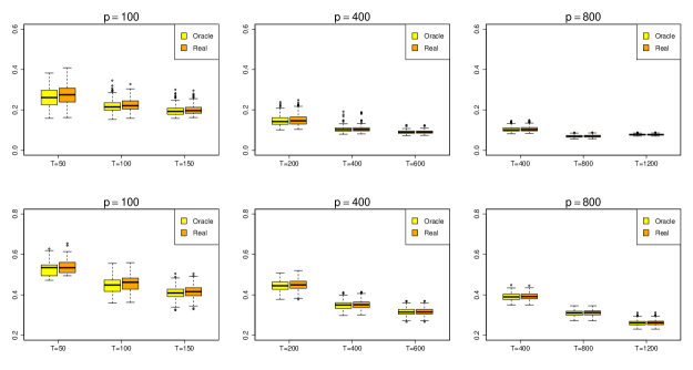
Figure 1: Boxplots of $\{D(\mathcal{M}(\widehat{{\bf A}}),\mathcal{M}({\bf A}))\}$ for Example 1 with stationary factor, and $\delta=0$ (3 top panels) and $\delta=0.5$ (3 bottom panels). Errors obtained using true D are marked with ‘oracle’, and using $\widehat{}\mbox{\bf D}$ are marked with ‘real’.

Example 1. Consider the linear model ${\bf y}_{t}={\bf D}{\bf z}_{t}+{\bf A}{\bf x}_{t}+\mbox{\boldmath$\varepsilon$}_{t}$, in which ${\bf z}_{t}$ follows the VAR(1) model:

$${\bf z}_{t}=\left(\begin{array}[]{cc}5/8&{1}/{8}\\ {1}/{8}&{5}/{8}\\ \end{array}\right){\bf z}_{t-1}+{\bf e}_{t},$$ (16)

where ${\bf e}_{t}\sim N({\bf 0},{\bf I}_{2})$. Let ${\bf D}$ be a $p\times 2$ matrix of which the elements were generated independently from the uniform distribution $U(-2,2)$, ${\bf x}_{t}$ be $3\times 1$ VAR(1) process with independent $N({\bf 0},{\bf I}_{3})$ innovations and the diagonal autoregressive coefficient matrix with 0.6, -0.5 and 0.3 as the main diagonal elements. This is a stationary factor process with $r=3$ factors. The elements of ${\bf A}$ were drawn independently from $U(-2,2)$ resulting a strong factor case with $\delta=0$. Also we considered a weak factor case with $\delta=0.5$ for which randomly selected $p-\lfloor{p^{1/2}\rfloor}$ elements in each column of ${\bf A}$ were set to 0. Let $\mbox{\boldmath$\varepsilon$}_{t}$ be independent and $N({\bf 0},{\bf I}_{p})$. To show the impact of the estimated coefficients matrix ${\widehat{}\mbox{\bf D}}$ on the estimation for the factors, we also report the results from using the true ${\bf D}$. We report the results with $\bar{k}=1$ only, since the results with $1\leq\bar{k}\leq 10$ are similar. The relative frequency estimates of $P(\widehat{r}=r)$ are reported in Table 1. It shows that the defect in estimating $r$ due to the errors in estimating D is almost negligible. Fig.1 displays the boxplots of the estimation errors $\{D(\mathcal{M}(\widehat{{\bf A}}),\mathcal{M}({\bf A}))\}$. Again the performance with the estimated coefficient matrix $\widehat{}\mbox{\bf D}$ is only slightly worse than that with the true D. When the factors are weaker (i.e. when $\delta=0.5$), it is harder to estimate both the number of factors and the factor loading space. All those findings are in line with the asymptotic results presented in Section 2.3.

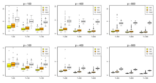
Figure 2: Boxplots of $p^{-1/2}\|\widehat{\bf D}-{\bf D}\|_{F}$ for Example 1 with endogeneity, and $\delta=0$ (3 top panels) and $\delta=0.5$ (3 bottom panels).

center

Table 2: Relative frequency estimates of $P(\widehat{r}=r)$ for Example 1 with endogeneity.

		$p$	$100$	$200$	$400$	$600$	$800$
	IV$2$	$T=0.5p$	0.660	0.885	0.995	0.995	1
		$T=p$	0.855	0.990	1	1	1
		$T=1.5p$	0.960	1	1	1	1
	IV$4$	$T=0.5p$	0.590	0.865	0.975	0.970	0.965
$\delta=0$		$T=p$	0.845	0.970	0.970	0.990	0.985
		$T=1.5p$	0.930	0.990	0.980	0.970	0.975
	OLS	$T=0.5p$	0.580	0.865	0.990	1	1
		$T=p$	0.855	0.980	1	1	1
		$T=1.5p$	0.945	1	1	0.995	1
	IV$2$	$T=0.5p$	0.280	0.665	0.625	0.630	0.620
		$T=p$	0.600	0.715	0.980	1	1
		$T=1.5p$	0.550	0.980	0.990	1	1
	IV$4$	$T=0.5p$	0.205	0.570	0.550	0.605	0.550
$\delta=0.5$		$T=p$	0.510	0.650	0.890	0.960	0.925
		$T=1.5p$	0.580	0.915	0.950	0.935	0.940
	OLS	$T=0.5p$	0.225	0.405	0.635	0.625	0.640
		$T=p$	0.535	0.705	1	1	0.995
		$T=1.5p$	0.630	0.955	1	1	0.995

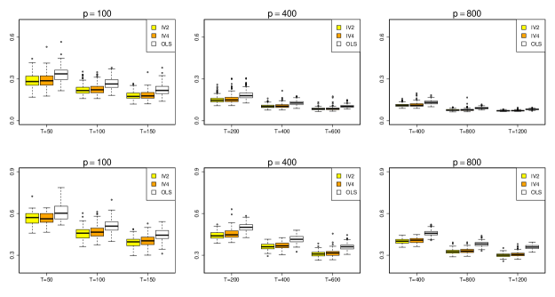
Figure 3: Boxplots of $\{D(\mathcal{M}(\widehat{{\bf A}}),\mathcal{M}({\bf A}))\}$ for Example 1 with endogeneity, and $\delta=0$ (3 top panels) and $\delta=0.5$ (3 bottom panels).

Now we consider the case with the endogeneity. To this end, we changed the definition for the regressor process $\mbox{\bf z}_{t}$ in the above setting. Instead of (16), we let

$$z_{1,t}=0.1x_{1,t}+0.1u_{t}+0.1u_{t}^{2},\quad z_{2,t}=0.1x_{2,t}-0.1u_{t}+0.1u_{t}^{2},$$

where $u_{t}$ is an AR(1) process defined by $u_{t}=0.5u_{t-1}+\epsilon_{t}$ and $\epsilon_{t}\sim N(0,1)$. The ordinary least squares estimator of ${\bf D}$ is no longer consistent now. We employ two different instrument variables ${\bf w}_{t}=(u_{t},u_{t}^{2})^{{\mathrm{\scriptscriptstyle T}}}$ and $\widetilde{{\bf w}}_{t}=(u_{t},u_{t}^{2},u_{t}^{3},u_{t}^{4})^{{\mathrm{\scriptscriptstyle T}}}$, as they are correlated with ${\bf z}_{t}$ but uncorrelated with ${\bf x}_{t}$ and $\mbox{\boldmath$\varepsilon$}_{t}$. The estimation error for $\widehat{{\bf D}}$ is measured by the normalized Frobenius norm $p^{-{1}/{2}}\|\widehat{{\bf D}}-{\bf D}\|_{F}$. Setting ${\bf R}={\bf I}_{2}$ for ${\bf w}_{t}$ and the elements of $\widetilde{\bf R}$ are generated from $U(-2,2)$ for $\widetilde{{\bf w}}_{t}$ in (13), we computed first both the ordinary least squares (OLS) estimates and the instrument variable method (IV) estimates for D, and then the estimates for the number of factors $r$ and the factor loading matrix A based on, respectively, the two sets of residuals resulted from the two regression estimation methods. The results are reported in Figs.2 and 3 and Table 2 where IV2 and IV4 represent the estimation using ${{\bf w}}_{t}$ and $\widetilde{{\bf w}}_{t}$ respectively. Those simulation results reinforce the findings in Section 3, which indicate that the existence of the endogeneity has no impact in identifying and in estimating the factor loading space. More precisely, Fig.2 shows that the errors $p^{-{1}/{2}}\|\widehat{{\bf D}}-{\bf D}\|_{F}$ for the OLS method are unusually large, as it effectively estimates $\mbox{\bf D}^{\star}$ in (11) instead of D. On the other hand, the IV method provides accurate estimates for D. However the differences of the two methods on the subsequent estimation for the number of factors $r$ and the factor loading space $\mathcal{M}(\mbox{\bf A})$ are small; see Table 2 and Fig.3. Since the IV method uses extra information, it tends to offer slightly better performance. Nevertheless Table 2 indicates that this improvement in estimating $r$ is almost negligible. Also, the results are not sensitive to the choice of R as long as the instrument variables are properly selected.

Table 3: Relative frequency estimates of $P(\widehat{r}=r)$ for Example 1 with nonstationary factors.

		$p$	$100$	$200$	$400$	$600$	$800$
$\delta=0$	D known	$T=0.5p$	0.155	0.525	0.855	0.925	0.970
		$T=p$	0.465	0.800	0.940	0.990	0.990
		$T=1.5p$	0.625	0.890	0.995	0.985	1
	D unknown	$T=0.5p$	0.110	0.525	0.835	0.920	0.970
		$T=p$	0.430	0.780	0.940	0.990	0.990
		$T=1.5p$	0.595	0.890	0.995	0.985	1
$\delta=0.5$	D known	$T=0.5p$	0	0.070	0.175	0.385	0.525
		$T=p$	0.025	0.235	0.535	0.705	0.765
		$T=1.5p$	0.145	0.475	0.740	0.815	0.860
	D unknown	$T=0.5p$	0	0.055	0.160	0.380	0.520
		$T=p$	0.025	0.215	0.520	0.685	0.760
		$T=1.5p$	0.125	0.465	0.740	0.805	0.850

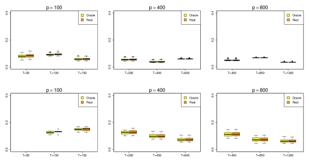
Figure 4: Boxplots of $\{D(\mathcal{M}(\widehat{{\bf A}}),\mathcal{M}({\bf A}))\}$ for Example 1 with nonstationary factors, and $\delta=0$ (3 top panels) and $\delta=0.5$ (3 bottom panels). Errors obtained using true D are marked with ‘oracle’, and using $\widehat{}\mbox{\bf D}$ are marked with ‘real’.

Now we consider the model with nonstationary factors $\mbox{\bf x}_{t}=3(x_{1,t},x_{2,t},x_{3,t})^{{\mathrm{\scriptscriptstyle T}}}$:

$$x_{1,t}-2t/T=0.8(x_{1,T-1}-2t/T)+e_{1,t},\quad x_{2,t}=3t/T,\quad x_{3,t}=x_{3,t-1}+\sqrt{\frac{10}{T}}e_{3,t},$$ (17)

where $e_{j,t}$ are independent and $N(0,1)$. The other settings are the same as the first part of this example. The results are reported in Table 3 and Fig.4. The patterns are similar to those in Table 1 and Fig.1, except that for a fixed $p$, the performance does not necessarily improve when the sample size $T$ increases; see Fig.4. This is due to the nonstationary nature of the factors defined in (17): new observations bring in the information on the new and time-varying underlying structure as far as the factor processes are concerned.

Table 4: Relative frequency estimates of $P(\widehat{r}=r)$ for Example 2 (with nonlinear regression).

		$p$	$100$	$200$	$400$	$600$	$800$
$\delta=0$	${\bf g}$ known	$T=0.5p$	0.780	0.865	0.965	0.975	0.985
		$T=p$	0.840	0.920	0.990	1	1
		$T=1.5p$	0.820	0.990	1	1	1
	${\bf g}$ unknown	$T=0.5p$	0.750	0.860	0.955	0.975	0.980
		$T=p$	0.830	0.890	0.990	1	1
		$T=1.5p$	0.780	0.990	1	1	1
$\delta=0.5$	${\bf g}$ known	$T=0.5p$	0.270	0.665	0.725	0.430	0.650
		$T=p$	0.390	0.700	0.850	0.810	0.800
		$T=1.5p$	0.390	0.720	0.885	0.960	1
	${\bf g}$ unknown	$T=0.5p$	0.260	0.625	0.665	0.390	0.600
		$T=p$	0.390	0.655	0.760	0.810	0.795
		$T=1.5p$	0.335	0.700	0.875	0.950	1

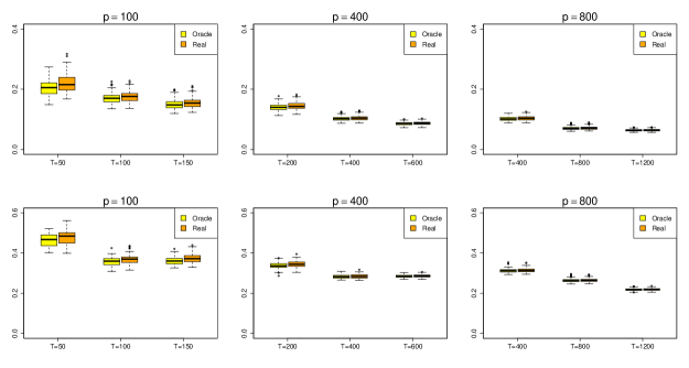
Figure 5: Boxplots of $\{D(\mathcal{M}(\widehat{{\bf A}}),\mathcal{M}({\bf A}))\}$ for Example 2 with nonlinear regression, and $\delta=0$ (3 top panels) and $\delta=0.5$ (3 bottom panels). Errors obtained using true ${\bf g}$ are marked with ‘oracle’, and using $\widehat{\bf g}$ are marked with ‘real’.

Example 2. We now consider a model with nonlinear regression function. Let $\mbox{\bf u}_{t}=u_{t}$ be a univariate AR(1) process defined by $u_{t}=0.5u_{t-1}+e_{t}$ with independent $N(0,1)$ innovations $e_{t}$. The nonlinear regression function ${\bf g}(u_{t})=(g_{1}(u_{t}),\ldots,g_{p}(u_{t}))^{{\mathrm{\scriptscriptstyle T}}}$ was defined as

$$g_{i}(u_{t})=\frac{\exp(\alpha_{i}^{(1)}u_{t})}{1+\exp(\alpha_{i}^{(1)}u_{t})},~{}~{}i=1,\ldots,\frac{p}{2}~{}~{}\text{and}~{}~{}g_{i}(u_{t})=\sin(\alpha_{i}^{(2)}u_{t}),~{}~{}i=\frac{p}{2}+1,\ldots,p,$$

where the parameters $\alpha_{i}^{(1)}$ were drawn independently from $N(0,4)$, and $\alpha_{i}^{(2)}$ were drawn independently from $U(-2,2)$ respectively. We used the same $\mbox{\bf A},\mbox{\bf x}_{t}$ and $\mbox{\boldmath$\varepsilon$}_{t}$ as in the first part of Example 1.

We used the polynomial expansion to approximate ${\bf g}(u_{t})$, i.e. $g_{i}(u_{t})\approx\sum_{j=1}^{m}d_{i,j}l_{j}(u_{t})$ with $l_{j}(u_{t})=u_{t}^{j-1}$, where the order $m$ was set as $\lfloor 2T^{1/5}\rfloor$. We obtained $\hat{d}_{i,j}$ by the least square estimation. Put $\widehat{{\bf g}}(u_{t})=(\hat{g}_{1}(u_{t}),\ldots,\hat{g}_{p}(u_{t}))^{{\mathrm{\scriptscriptstyle T}}}$ for $\hat{g}_{i}(u_{t})=\sum_{j=1}^{m}\hat{d}_{i,j}l_{j}(u_{t})$. The residuals $\widehat{\mbox{\boldmath$\eta$}}_{t}={\bf y}_{t}-\widehat{{\bf g}}({\bf u}_{t})$ were then used to estimate the latent factors. We set $\bar{k}=\lfloor 2T^{1/5}\rfloor$; see Theorem 4.2. The simulation results are reported in Table 4 and Fig.5, which present similar patterns as in the first part of Example 1.

6 Real data analysis

We illustrate our method by modeling the daily returns of $123$ stocks from $2$ January 2002 to 11 July 2008. The stocks were selected among those contained in the S&P$500$ which were traded everyday during this period. The returns were calculated based on the daily close prices. We have in total $T=1642$ observations with the dimension $p=123$. This data has been analyzed in Lam and Yao (2012). They identified two factors under a pure factor model setting, i.e. model (1) with ${\bf z}_{t}\equiv\bf 0$. Furthermore the estimated factor loading space contains the return of the S&P$500$. Hence it can be regarded as one of the two factors. Since the S&P$500$ index is often viewed as a proxy of the market index, it is reasonable to take its return as a known factor $z_{t}$ in our model (1). We calculated the ordinary least square estimator for the regression coefficient matrix ${\bf D}$ which is now a $123\times 1$ vector with each element representing the impact of the S&P$500$ index to the return of the corresponding stock. As all the estimated elements are positive, indicating the positive correlations between the returns of market index and the those 123 stocks.

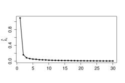
(a) The eigenvalues of $\widehat{{\bf M}}$

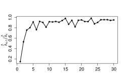
(b) Ratio of the eigenvalues of $\widehat{{\bf M}}$

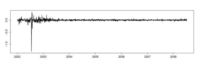
(c) The estimated latent factor

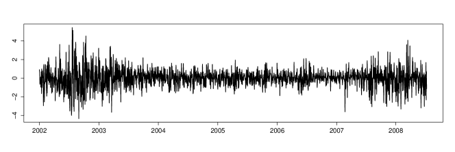
(d) S&P $500$ returns

Figure 6: The estimated eigenvalues (multiplied by $10^{6}$), the ratio of eigenvalues, the estimated latent factor and the S&P$500$ returns in 2 January 2002 – 11 July 2008.

Fig.6(d) displays the first $30$ eigenvalues of $\widehat{{\bf M}}$, defined as in (6) with $\bar{k}=1$, sorted in the descending order. The ratio of $\widehat{\lambda}_{i+1}/\widehat{\lambda}_{i}$ in the right panel indicates that there is only one latent factor. Varying $\bar{k}$ between 1 to 20 did not alter this result. Fig.6(d)(c) shows that the sparks of the estimated factor process occur around $22$ July, 2002, which is consistent with the oscillations of S&P500 index, although the S&P$500$ are less volatile. The autocorrelations of the estimated factors $\widehat{\gamma}_{j}^{{\mathrm{\scriptscriptstyle T}}}({\bf y}_{t}-\widehat{\bf D}{\bf z}_{t})$, where $\widehat{\gamma}_{j}$ is the unit eigenvector of $\widehat{{\bf M}}$ corresponding to its $j$th largest eigenvalue, are plotted in Fig.7 for $j=1,2,3$. The autocorrelations of the first factor is significant non-zero. On the other hand, there are hardly any significant non-zero autocorrelations for both the second and the third factors.

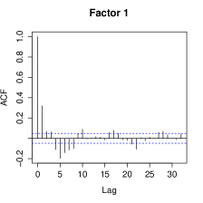
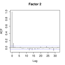
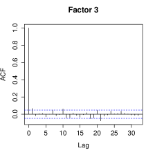
Figure 7: The ACFs of the first three estimated factors.

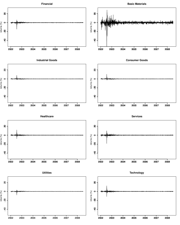
Figure 8: The estimated latent part ${\bf A}{\bf x}_{t}$ across different sectors.

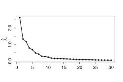
(a) The eigenvalues of $\widehat{{\bf M}}$

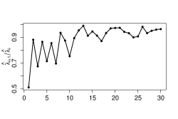
(b) Ratio of the eigenvalues of $\widehat{{\bf M}}$

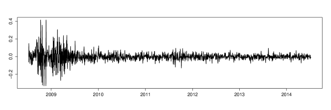
(c) The estimated latent factor

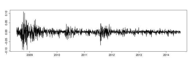
(d) S&P $500$ returns

Figure 9: The estimated eigenvalues (multiplied by $10^{6}$), the ratio of eigenvalues, the estimated latent factor and the S&P$500$ returns in 14 July 2008 – 11 July 2014.

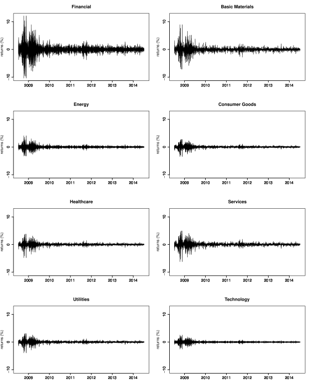
Figure 10: The estimated latent part ${\bf A}{\bf x}_{t}$ across different sectors.

To gain some appreciation of the latent factor, we divide the $123$ stocks into eight sectors: Financial, Basic Materials, Industrial Goods, Consumer Goods, Healthcare, Services, Utilities and Technology. We estimated the latent factor for each of those eight sectors. Those estimated sector factors are plotted in Fig.8. We observe that those estimated sector factors behave differently for the different sectors. Especially the Basic Materials sector exhibits the largest fluctuation. Consequently, we may deduce that the oscillations, especially the sparks, of the estimated factor in Fig.6(d)(c) are largely due to changes in the Basic Materials sector. This is consistent with the relevant economics and finance principles. Basic Materials sector includes mainly the stocks of energy companies such as oil, gas, coal et al. The energy, especially oil, is the foundation for economic and social development. Hence, the changes in oil price are often considered as important events which underpin stock market fluctuations, see, e.g. Jones and Kaul (1996) and Kilian and Park (2009). During January 2002 to December 2003, international oil price had a huge increase. It rose $19\%$ from the average in 2002. The 2003 invasion of Iraq marks a significant event as Iraq possesses a significant portion of the global oil reserve. Hence, the returns of the Basic Materials sector oscillate dramatically during that period. Among other sectors, Industrial and Consumer Goods have similar behaviors. However, the returns of both the sectors have little changes around zero, thus they have little contributions to the estimated factor. The same arguments hold for the Utilities sector. Also note that the returns for the Financial, Healthcare, Services and Technology sectors are much less volatile in comparison to that of the Basic Materials sector. We may conclude that, the estimated factor mainly reflects the feature of stocks in Basic Materials sector. The factor also contains some market information about the Financial, Healthcare, Services and Technology sectors, but less so on the Industrial Goods, Consumer Goods and Utilities sectors.

We repeat the above exercise for another set of return data in 14 July 2008 – 11 July 2014 from the 196 stocks contained in S&P$500$. Now $T=1510$ and $p=196$. The ratios of $\widehat{\lambda}_{i+1}/\widehat{\lambda}_{i}$ shown in Fig.9(b) indicate that there is still only one latent factor, in addition to S&P$500$. The estimated latent factor shown in Fig.9(c) fluctuated widely around 2009, which is consistent with the pronounced decline the stock market due to the global financial crisis. While the latent factor process seems to resemble the returns of S&P$500$ (see Figs.9(c) and (d)), the two series are orthogonal with each other (with the sample correlation coefficient equal to 0.00047). The estimated factors for each of the eight sectors are plotted in Fig.10. In contrast to the findings in 2002-2008, all the eight sectors contributed to the fluctuation around 2009, though the financial sector was most predominant. The crisis caused by the sharp down-turn of financial industry in early 2009 impacted all sectors in the society.

Appendix

Throughout the Appendix, we use $C$s to denote generic uniformly positive constants only depends on the parameters $C_{i}$s appear in the technical conditions which may be different in different uses. Meanwhile, we denote ${\bf A}{\bf x}_{t}$ by $\mbox{\boldmath$\zeta$}_{t}$. We first present the following lemmas which are used in proofs of the propositions and theorems.

Lemma 6.1.

Under Conditions 2.1-2.2, $\|T^{-1}\sum_{t=1}^{T}\{{\bf z}_{t}{\bf z}_{t}^{\mathrm{\scriptscriptstyle T}}-E({\bf z}_{t}{\bf z}_{t}^{\mathrm{\scriptscriptstyle T}})\}\|_{F}=O_{p}(mT^{-1/2}).$

Proof: For any $i,j=1,\ldots,m$, by Cauchy-Schwarz inequality and Davydov inequality,

$$\begin{split}&~{}E\bigg{[}\bigg{|}\frac{1}{T}\sum_{t=1}^{T}\{z_{i,t}z_{j,t}-E(z_{i,t}z_{j,t})\}\bigg{|}^{2}\bigg{]}\\ =&~{}\frac{1}{T^{2}}\sum_{t=1}^{T}E[\{z_{i,t}z_{j,t}-E(z_{i,t}z_{j,t})\}^{2}]\\ &+\frac{1}{T^{2}}\sum_{t_{1}\neq t_{2}}E[\{z_{i,t_{1}}z_{j,t_{1}}-E(z_{i,t_{1}}z_{j,t_{1}})\}\{z_{i,t_{2}}z_{j,t_{2}}-E(z_{i,t_{2}}z_{j,t_{2}})\}]\\ \leq&~{}\frac{C}{T}+\frac{C}{T^{2}}\sum_{t_{1}\neq t_{2}}\alpha(|t_{1}-t_{2}|)^{1-2/\gamma}\leq\frac{C}{T}+\frac{C}{T}\sum_{u=1}^{T}\alpha(u)^{1-2/\gamma}.\end{split}$$ (18)

Then, $E\{\|T^{-1}\sum_{t=1}^{T}\{{\bf z}_{t}{\bf z}_{t}^{\mathrm{\scriptscriptstyle T}}-E({\bf z}_{t}{\bf z}_{t}^{\mathrm{\scriptscriptstyle T}})\}\|_{F}^{2}\}=O(m^{2}T^{-1})$ which implies the result. $\hfill\Box$

Proof of Proposition 2.1: Note that $(\widehat{{\bf D}}-{\bf D})^{\mathrm{\scriptscriptstyle T}}=(T^{-1}\sum_{t=1}^{T}{\bf z}_{t}{\bf z}_{t}^{\mathrm{\scriptscriptstyle T}})^{-1}(T^{-1}\sum_{t=1}^{T}{\bf z}_{t}\mbox{\boldmath$\eta$}_{t}^{\mathrm{\scriptscriptstyle T}})$ and $\lambda_{\min}(T^{-1}\sum_{t=1}^{T}{\bf z}_{t}{\bf z}_{t}^{\mathrm{\scriptscriptstyle T}})$ is bounded away from zero with probability approaching one, which is implied by Condition 2.3 and Lemma 6.1, then $\|\widehat{{\bf D}}-{\bf D}\|_{F}=O_{p}(\|T^{-1}\sum_{t=1}^{T}{\bf z}_{t}\mbox{\boldmath$\eta$}_{t}^{\mathrm{\scriptscriptstyle T}}\|_{F})$. For each $i=1,\ldots,m$ and $j=1,\ldots,p$, from $\textrm{cov}({\bf z}_{t},\mbox{\boldmath$\eta$}_{t})={\bf 0}$ and similar to (18), we can obtain $E\{(T^{-1}\sum_{t=1}^{T}z_{i,t}\eta_{j,t})^{2}\}\leq CT^{-1}$. Then, $E\{\|T^{-1}\sum_{t=1}^{T}{\bf z}_{t}\mbox{\boldmath$\eta$}_{t}^{\mathrm{\scriptscriptstyle T}}\|_{F}^{2}\}=O(pT^{-1})$. Hence, $\|\widehat{{\bf D}}-{\bf D}\|_{F}=O_{p}(p^{1/2}T^{-1/2})$. $\hfill\square$

Lemma 6.2.

Under Conditions 2.1-2.2, if $k=o(T)$, then

$$\|\widehat{\mbox{\boldmath$\Sigma$}}_{\eta}(k)-\mbox{\boldmath$\Sigma$}_{\eta}(k)\|_{F}=\|{\bf D}-\widehat{{\bf D}}\|_{F}^{2}J_{1,k}+\|{\bf D}-\widehat{{\bf D}}\|_{F}J_{2,k}+J_{3,k}$$

where $E(J_{1,k}^{2})\leq Ckm^{2}(T-k)^{-1}+Cm^{2}\alpha(k)^{2-4/\gamma}$, $E(J_{2,k}^{2})\leq Ckpm(T-k)^{-1}+Cpm\alpha(k)^{2-4/\gamma}$ and $E(J_{3,k}^{2})\leq Ckp^{2}(T-k)^{-1}$.

Proof: For each $k=o(T)$,

$$\begin{split}\widehat{\mbox{\boldmath$\Sigma$}}_{\eta}(k)-\mbox{\boldmath$\Sigma$}_{\eta}(k)=&~{}\frac{1}{T-k}\sum_{t=1}^{T-k}(\widehat{\mbox{\boldmath$\eta$}}_{t+k}\widehat{\mbox{\boldmath$\eta$}}_{t}^{\mathrm{\scriptscriptstyle T}}-\mbox{\boldmath$\eta$}_{t+k}\mbox{\boldmath$\eta$}_{t}^{\mathrm{\scriptscriptstyle T}})+\frac{1}{T-k}\sum_{t=1}^{T-k}\{\mbox{\boldmath$\eta$}_{t+k}\mbox{\boldmath$\eta$}_{t}^{\mathrm{\scriptscriptstyle T}}-E(\mbox{\boldmath$\eta$}_{t+k}\mbox{\boldmath$\eta$}_{t}^{\mathrm{\scriptscriptstyle T}})\}\\ &~{}+\bar{\mbox{\boldmath$\eta$}}\bar{\mbox{\boldmath$\eta$}}^{\mathrm{\scriptscriptstyle T}}-\frac{1}{T-k}\sum_{t=1}^{T-k}\widehat{\mbox{\boldmath$\eta$}}_{t+k}\bar{\mbox{\boldmath$\eta$}}^{\mathrm{\scriptscriptstyle T}}-\frac{1}{T-k}\sum_{t=1}^{T-k}\bar{\mbox{\boldmath$\eta$}}\widehat{\mbox{\boldmath$\eta$}}_{t}^{\mathrm{\scriptscriptstyle T}}\\ =&~{}I_{1,k}+I_{2,k}+I_{3,k}+I_{4,k}+I_{5,k}.\end{split}$$

As

$$\begin{split}I_{1,k}=&~{}({\bf D}-\widehat{{\bf D}})\bigg{(}\frac{1}{T-k}\sum_{t=1}^{T-k}{\bf z}_{t+k}{\bf z}_{t}^{\mathrm{\scriptscriptstyle T}}\bigg{)}({\bf D}-\widehat{{\bf D}})^{\mathrm{\scriptscriptstyle T}}+({\bf D}-\widehat{{\bf D}})\bigg{(}\frac{1}{T-k}\sum_{t=1}^{T-k}{\bf z}_{t+k}\mbox{\boldmath$\eta$}_{t}^{\mathrm{\scriptscriptstyle T}}\bigg{)}\\ &+\bigg{(}\frac{1}{T-k}\sum_{t=1}^{T-k}\mbox{\boldmath$\eta$}_{t+k}{\bf z}_{t}^{\mathrm{\scriptscriptstyle T}}\bigg{)}({\bf D}-\widehat{{\bf D}})^{\mathrm{\scriptscriptstyle T}},\\ \end{split}$$

then

$$\begin{split}\|I_{1,k}\|_{F}\leq&~{}\|{\bf D}-\widehat{{\bf D}}\|_{F}^{2}\bigg{\|}\frac{1}{T-k}\sum_{t=1}^{T-k}{\bf z}_{t+k}{\bf z}_{t}^{\mathrm{\scriptscriptstyle T}}\bigg{\|}_{F}+\|{\bf D}-\widehat{{\bf D}}\|_{F}\bigg{\|}\frac{1}{T-k}\sum_{t=1}^{T-k}{\bf z}_{t+k}\mbox{\boldmath$\eta$}_{t}^{\mathrm{\scriptscriptstyle T}}\bigg{\|}_{F}\\ &+\|{\bf D}-\widehat{{\bf D}}\|_{F}\bigg{\|}\frac{1}{T-k}\sum_{t=1}^{T-k}\mbox{\boldmath$\eta$}_{t+k}{\bf z}_{t}^{\mathrm{\scriptscriptstyle T}}\bigg{\|}_{F}.\end{split}$$

For any $i,j=1,\ldots,m$,

$$\begin{split}E\bigg{\{}\bigg{(}\frac{1}{T-k}\sum_{t=1}^{T-k}z_{i,t+k}z_{j,t}\bigg{)}^{2}\bigg{\}}\leq 2E\bigg{(}\bigg{[}\frac{1}{T-k}\sum_{t=1}^{T-k}\{z_{i,t+k}z_{j,t}-E(z_{i,t+k}z_{j,t})\}\bigg{]}^{2}\bigg{)}+2\max_{t}\{E(z_{i,t+k}z_{j,t})\}^{2}.\end{split}$$

By Cauchy-Schwarz inequality and Davydov inequality,

$$\begin{split}&~{}E\bigg{(}\bigg{[}\frac{1}{T-k}\sum_{t=1}^{T-k}\{z_{i,t+k}z_{j,t}-E(z_{i,t+k}z_{j,t})\}\bigg{]}^{2}\bigg{)}\\ =&~{}\frac{1}{(T-k)^{2}}\sum_{t=1}^{T-k}E[\{z_{i,t+k}z_{j,t}-E(z_{i,t+k}z_{j,t})\}^{2}]\\ &+\frac{1}{(T-k)^{2}}\sum_{t_{1}\neq t_{2}}E[\{z_{i,t_{1}+k}z_{j,t_{1}}-E(z_{i,t_{1}+k}z_{j,t_{1}})\}\{z_{i,t_{2}+k}z_{j,t_{2}}-E(z_{i,t_{2}+k}z_{j,t_{2}})\}]\\ \leq&~{}\frac{C}{T-k}+\frac{Ck}{T-k}+\frac{Ck(k-1)}{(T-k)^{2}}+\frac{C}{T-k}\sum_{u=1}^{T-2k-1}\alpha(u)^{1-2/\gamma}.\\ \end{split}$$ (19)

and $\{E(z_{i,t+k}z_{j,t})\}^{2}\leq C\alpha(k)^{2-4/\gamma}$. Then, $E[\{(T-k)^{-1}\sum_{t=1}^{T-k}z_{i,t+k}z_{j,t}\}^{2}]\leq Ck(T-k)^{-1}+C\alpha(k)^{2-4/\gamma}$. Thus, $E\{\|(T-k)^{-1}\sum_{t=1}^{T-k}{\bf z}_{t+k}{\bf z}_{t}^{\mathrm{\scriptscriptstyle T}}\|_{F}^{2}\}\leq Ckm^{2}(T-k)^{-1}+Cm^{2}\alpha(k)^{2-4/\gamma}.$ By the same argument, we can obtain $E\{\|(T-k)^{-1}\sum_{t=1}^{T-k}{\bf z}_{t+k}\mbox{\boldmath$\eta$}_{t}^{\mathrm{\scriptscriptstyle T}}\|_{F}^{2}\}\leq Ckpm(T-k)^{-1}+Cpm\alpha(k)^{2-4/\gamma}$ and $E\{\|(T-k)^{-1}\sum_{t=1}^{T-k}\mbox{\boldmath$\eta$}_{t+k}{\bf z}_{t}^{\mathrm{\scriptscriptstyle T}}\|_{F}^{2}\}\leq Ckpm(T-k)^{-1}+Cpm\alpha(k)^{2-4/\gamma}$. Hence, $\|I_{1,k}\|_{F}=\|{\bf D}-\widehat{{\bf D}}\|_{F}^{2}J_{1,k}+\|{\bf D}-\widehat{{\bf D}}\|_{F}J_{2,k}$ where $E(J_{1,k}^{2})\leq Ckm^{2}(T-k)^{-1}+Cm^{2}\alpha(k)^{2-4/\gamma}$ and $E(J_{2,k}^{2})\leq Ckpm(T-k)^{-1}+Cpm\alpha(k)^{2-4/\gamma}$. On the other hand, similar to (19), we can obtain $E(\|I_{2,k}\|_{F}^{2})\leq Ckp^{2}(T-k)^{-1}$. For $I_{3,k}$, we have $E(\|I_{3,k}\|_{F}^{2})\leq E(\|\bar{\mbox{\boldmath$\eta$}}\|_{2}^{4})$. By Jensen inequality and Davydov inequality, $E(\|I_{3,k}\|_{F}^{2})\leq Cp^{2}T^{-1}$. Following the same way, we have both $E(\|I_{4,k}\|_{F}^{2})$ and $E(\|I_{5,k}\|_{F}^{2})$ can be bounded by $Ckp^{2}(T-k)^{-1}$. Hence, we complete the proof. $\hfill\Box$

Lemma 6.3.

Under Condition 2.4, for $k=1,\ldots,\bar{k}$,

$$\|\mbox{\boldmath$\Sigma$}_{\eta}(k)\|_{2}\leq Cp^{1-\delta}+C\kappa_{2}.$$

Proof: Note that $\mbox{\boldmath$\Sigma$}_{\eta}(k)={\bf A}\mbox{\boldmath$\Sigma$}_{x}(k){\bf A}^{\mathrm{\scriptscriptstyle T}}+\mbox{\boldmath$\Sigma$}_{x\varepsilon}(k)$, then $\|\mbox{\boldmath$\Sigma$}_{\eta}(k)\|_{2}\leq\|{\bf A}\|_{2}^{2}\|\mbox{\boldmath$\Sigma$}_{x}(k)\|_{2}+\|\mbox{\boldmath$\Sigma$}_{x\varepsilon}(k)\|_{2}.$ From Condition 2.4, we complete the proof. $\hfill\Box$

Lemma 6.4.

Under Conditions 2.1-2.4,

$$\|\widehat{{\bf M}}-{\bf M}\|_{2}=O_{p}\{(p^{1-\delta}+\kappa_{2})pT^{-1/2}+p^{2}T^{-1}\}.$$

Proof: Note that

$$\begin{split}\|\widehat{{\bf M}}-{\bf M}\|_{2}\leq&~{}\sum_{k=1}^{\bar{k}}\|\widehat{\mbox{\boldmath$\Sigma$}}_{\eta}(k)-\mbox{\boldmath$\Sigma$}_{\eta}(k)\|_{2}^{2}+2\sum_{k=1}^{\bar{k}}\|\mbox{\boldmath$\Sigma$}_{\eta}(k)\|_{2}\|\widehat{\mbox{\boldmath$\Sigma$}}_{\eta}(k)-\mbox{\boldmath$\Sigma$}_{\eta}(k)\|_{2}=I_{1}+I_{2}.\\ \end{split}$$

By Lemmas 6.2 and 6.3, we can obtain

$$\begin{split}I_{1}\leq&~{}3\|{\bf D}-\widehat{{\bf D}}\|_{F}^{4}\sum_{k=1}^{\bar{k}}J_{1,k}^{2}+3\|{\bf D}-\widehat{{\bf D}}\|_{F}^{2}\sum_{k=1}^{\bar{k}}J_{2,k}^{2}+3\sum_{k=1}^{\bar{k}}J_{3,k}^{2}=O_{p}(p^{2}T^{-1})\end{split}$$

and

$$\begin{split}I_{2}\leq&~{}2\bigg{\{}\|{\bf D}-\widehat{{\bf D}}\|_{F}^{2}\sum_{k=1}^{\bar{k}}J_{1,k}+\|{\bf D}-\widehat{{\bf D}}\|_{F}\sum_{k=1}^{\bar{k}}J_{2,k}+\sum_{k=1}^{\bar{k}}J_{3,k}\bigg{\}}\sup_{1\leq k\leq\bar{k}}\|\mbox{\boldmath$\Sigma$}_{\eta}(k)\|_{2}\\ =&~{}O_{p}\{(p^{1-\delta}+\kappa_{2})pT^{-1/2}\}.\end{split}$$

Hence, we complete the proof. $\hfill\Box$

Lemma 6.5.

Under Condition 2.4,

$$\lambda_{r}({\bf M})\geq\left\{\begin{aligned} Cp^{2(1-\delta)},&~{}~{}\textrm{if}~{}\kappa_{2}=o(p^{1-\delta});\\ C\kappa_{1}^{2},&~{}~{}\textrm{if}~{}p^{1-\delta}=o(\kappa_{1}).\end{aligned}\right.$$

Proof: From (5), we know

$$\lambda_{r}({\bf M})=\lambda_{\min}\bigg{[}\sum_{k=1}^{\bar{k}}\{\mbox{\boldmath$\Sigma$}_{x}(k){\bf A}^{\mathrm{\scriptscriptstyle T}}+\mbox{\boldmath$\Sigma$}_{x\varepsilon}(k)\}\{\mbox{\boldmath$\Sigma$}_{x}(k){\bf A}^{\mathrm{\scriptscriptstyle T}}+\mbox{\boldmath$\Sigma$}_{x\varepsilon}(k)\}^{\mathrm{\scriptscriptstyle T}}\bigg{]}.$$

For each $k=1,\ldots,\bar{k}$,

$$\begin{split}&~{}\lambda_{\min}[\{\mbox{\boldmath$\Sigma$}_{x}(k){\bf A}^{\mathrm{\scriptscriptstyle T}}+\mbox{\boldmath$\Sigma$}_{x\varepsilon}(k)\}\{\mbox{\boldmath$\Sigma$}_{x}(k){\bf A}^{\mathrm{\scriptscriptstyle T}}+\mbox{\boldmath$\Sigma$}_{x\varepsilon}(k)\}^{\mathrm{\scriptscriptstyle T}}]\\ \asymp&~{}\left\{\begin{aligned} \lambda_{\min}\{\mbox{\boldmath$\Sigma$}_{x}(k)\mbox{\boldmath$\Sigma$}_{x}(k)^{\mathrm{\scriptscriptstyle T}}\},&~{}~{}\textrm{if}~{}\lambda_{\max}\{\mbox{\boldmath$\Sigma$}_{x\varepsilon}(k)\mbox{\boldmath$\Sigma$}_{x\varepsilon}(k)^{\mathrm{\scriptscriptstyle T}}\}=o(\lambda_{\min}\{\mbox{\boldmath$\Sigma$}_{x}(k)\mbox{\boldmath$\Sigma$}_{x}(k)^{\mathrm{\scriptscriptstyle T}}\});\\ \lambda_{\min}\{\mbox{\boldmath$\Sigma$}_{x\varepsilon}(k)\mbox{\boldmath$\Sigma$}_{x\varepsilon}(k)^{\mathrm{\scriptscriptstyle T}}\},&~{}~{}\textrm{if}~{}\lambda_{\max}\{\mbox{\boldmath$\Sigma$}_{x}(k)\mbox{\boldmath$\Sigma$}_{x}(k)^{\mathrm{\scriptscriptstyle T}}\}=o(\lambda_{\min}\{\mbox{\boldmath$\Sigma$}_{x\varepsilon}(k)\mbox{\boldmath$\Sigma$}_{x\varepsilon}(k)^{\mathrm{\scriptscriptstyle T}}\}).\\ \end{aligned}\right.\\ \end{split}$$

Notice Condition 2.4, then

$$\lambda_{\min}[\{\mbox{\boldmath$\Sigma$}_{x}(k){\bf A}^{\mathrm{\scriptscriptstyle T}}+\mbox{\boldmath$\Sigma$}_{x\varepsilon}(k)\}\{\mbox{\boldmath$\Sigma$}_{x}(k){\bf A}^{\mathrm{\scriptscriptstyle T}}+\mbox{\boldmath$\Sigma$}_{x\varepsilon}(k)\}^{\mathrm{\scriptscriptstyle T}}]\geq\left\{\begin{aligned} Cp^{2(1-\delta)},&~{}~{}\textrm{if}~{}\kappa_{2}=o(p^{1-\delta});\\ C\kappa_{1}^{2},&~{}~{}\textrm{if}~{}p^{1-\delta}=o(\kappa_{1}).\\ \end{aligned}\right.\\$$

Hence, we complete the proof.$\hfill\Box$

Proof of Theorem 2.1: By Lemma 6.5, $\|\widehat{{\bf M}}-{\bf M}\|_{2}=o_{p}\{\lambda_{r}({\bf M})\}$ provided that either case (i) $\kappa_{2}=o(p^{1-\delta})$ and $p^{2\delta}T^{-1}=o(1)$ or (ii) $p^{1-\delta}=o(\kappa_{1})$ and $\kappa_{1}^{-2}\kappa_{2}pT^{-1/2}=o(1)$ hold. By Lemma 3 of Lam et al. (2011), and using the same argument of the proof of Theorem 1 in their paper,

$$\begin{split}\|\widehat{{\bf A}}-{\bf A}\|_{2}=&~{}\left\{\begin{aligned} O_{p}(p^{\delta}T^{-1/2}),&~{}~{}\hbox{if $\kappa_{2}=o(p^{1-\delta})$ and $p^{2\delta}T^{-1}=o(1)$;}\\ O_{p}(\kappa_{1}^{-2}\kappa_{2}pT^{-1/2}),&~{}~{}\hbox{if $p^{1-\delta}=o(\kappa_{1})$ and $\kappa_{1}^{-2}\kappa_{2}pT^{-1/2}=o(1)$}.\end{aligned}\right.\end{split}$$

Hence, we complete the proof. $\hfill\Box$

Proof of Theorem 2.2: Note that

$$\begin{split}\widehat{{\bf A}}\widehat{{\bf x}}_{t}-{\bf A}{\bf x}_{t}=&~{}\widehat{{\bf A}}\widehat{}\mbox{\bf A}^{\mathrm{\scriptscriptstyle T}}{\bf A}{\bf x}_{t}+\widehat{{\bf A}}\widehat{}\mbox{\bf A}^{\mathrm{\scriptscriptstyle T}}\mbox{\boldmath$\varepsilon$}_{t}-{\bf A}{\bf x}_{t}+\widehat{{\bf A}}\widehat{}\mbox{\bf A}^{\mathrm{\scriptscriptstyle T}}(\widehat{\mbox{\boldmath$\eta$}}_{t}-\mbox{\boldmath$\eta$}_{t})\\ =&~{}(\widehat{{\bf A}}\widehat{}\mbox{\bf A}^{\mathrm{\scriptscriptstyle T}}-{\bf A}\mbox{\bf A}^{\mathrm{\scriptscriptstyle T}}){\bf A}{\bf x}_{t}+\widehat{{\bf A}}(\widehat{{\bf A}}-{\bf A})^{\mathrm{\scriptscriptstyle T}}\mbox{\boldmath$\varepsilon$}_{t}+\widehat{{\bf A}}\mbox{\bf A}^{\mathrm{\scriptscriptstyle T}}\mbox{\boldmath$\varepsilon$}_{t}+\widehat{{\bf A}}\widehat{}\mbox{\bf A}^{\mathrm{\scriptscriptstyle T}}(\widehat{\mbox{\boldmath$\eta$}}_{t}-\mbox{\boldmath$\eta$}_{t})\\ =&~{}I_{1}+I_{2}+I_{3}+I_{4}.\end{split}$$

For $I_{1}$, $\|I_{1}\|_{2}\leq 2\|\widehat{{\bf A}}-{\bf A}\|_{2}\|{\bf A}{\bf x}_{t}\|_{2}\leq O_{p}(p^{1/2}\|\widehat{{\bf A}}-{\bf A}\|_{2})$. For $I_{2}$, $\|I_{2}\|_{2}\leq\|\widehat{{\bf A}}-{\bf A}\|_{2}\|\mbox{\boldmath$\varepsilon$}_{t}\|_{2}=O_{p}(p^{1/2}\|\widehat{{\bf A}}-{\bf A}\|_{2}).$ For $I_{3}$, as $E(\|I_{3}\|_{2}^{2})=\sum_{i=1}^{r}E\{({\bf a}_{i}^{\mathrm{\scriptscriptstyle T}}\mbox{\boldmath$\varepsilon$}_{t})^{2}\}\leq r\lambda_{\max}(\mbox{\boldmath$\Sigma$}_{\varepsilon})$, then $I_{3}=O_{p}(1).$ For $I_{4}$, by Proposition 2.1, $\|I_{4}\|_{2}\leq\|\widehat{{\bf D}}-{\bf D}\|_{2}\|{\bf z}_{t}\|_{2}=O_{p}(p^{1/2}T^{-1/2}).$ Hence, $p^{-1/2}\|\widehat{{\bf A}}\widehat{{\bf x}}_{t}-{\bf A}{\bf x}_{t}\|_{2}\leq O_{p}(\|\widehat{{\bf A}}-{\bf A}\|_{2}+p^{-1/2}+T^{-1/2}).$ $\hfill\Box$

Proof of Theorem 2.3: Let $\mbox{\boldmath$\Sigma$}_{\zeta}(k)=(T-k)^{-1}\sum_{t=1}^{T-k}\textrm{cov}(\mbox{\boldmath$\zeta$}_{t+k},\mbox{\boldmath$\zeta$}_{t})$, then $\mbox{\boldmath$\Sigma$}_{\zeta}(k)={\bf A}\mbox{\boldmath$\Sigma$}_{x}(k){\bf A}^{\mathrm{\scriptscriptstyle T}}$. Note that

$$\begin{split}\textrm{tr}\{\mbox{\boldmath$\Sigma$}_{\zeta}(1)^{\mathrm{\scriptscriptstyle T}}(I_{p}-\widehat{{\bf A}}\widehat{\bf A}^{\mathrm{\scriptscriptstyle T}})\mbox{\boldmath$\Sigma$}_{\zeta}(1)\}=&~{}\textrm{tr}\{\mbox{\boldmath$\Sigma$}_{x}(1)^{\mathrm{\scriptscriptstyle T}}(I_{r}-{\bf A}^{\mathrm{\scriptscriptstyle T}}\widehat{{\bf A}}\widehat{\bf A}^{\mathrm{\scriptscriptstyle T}}{\bf A})\mbox{\boldmath$\Sigma$}_{x}(1)\}\\ \geq&~{}\textrm{tr}(I_{r}-{\bf A}^{\mathrm{\scriptscriptstyle T}}\widehat{{\bf A}}\widehat{{\bf A}}^{\mathrm{\scriptscriptstyle T}}{\bf A})\lambda_{\min}\{\mbox{\boldmath$\Sigma$}_{x}(1)\mbox{\boldmath$\Sigma$}_{x}(1)^{\mathrm{\scriptscriptstyle T}}\}\\ =&~{}r\{D(\mathcal{M}(\widehat{{\bf A}}),\mathcal{M}({\bf A}))\}^{2}\lambda_{\min}\{\mbox{\boldmath$\Sigma$}_{x}(1)\mbox{\boldmath$\Sigma$}_{x}(1)^{\mathrm{\scriptscriptstyle T}}\}.\end{split}$$

By Condition 2.4,

$$\textrm{tr}\{\mbox{\boldmath$\Sigma$}_{\zeta}(1)^{\mathrm{\scriptscriptstyle T}}(I_{p}-\widehat{{\bf A}}\widehat{{\bf A}}^{\mathrm{\scriptscriptstyle T}})\mbox{\boldmath$\Sigma$}_{\zeta}(1)\}\geq Cp^{2(1-\delta)}\{D(\mathcal{M}(\widehat{{\bf A}}),\mathcal{M}({\bf A}))\}^{2}.$$

At the same time,

$$\begin{split}&~{}\textrm{tr}\{\mbox{\boldmath$\Sigma$}_{\zeta}(1)^{\mathrm{\scriptscriptstyle T}}(I_{p}-\widehat{{\bf A}}\widehat{{\bf A}}^{\mathrm{\scriptscriptstyle T}})\mbox{\boldmath$\Sigma$}_{\zeta}(1)\}-\textrm{tr}\{\mbox{\boldmath$\Sigma$}_{\zeta}(1)^{\mathrm{\scriptscriptstyle T}}(I_{p}-{\bf A}{\bf A}^{\mathrm{\scriptscriptstyle T}})\mbox{\boldmath$\Sigma$}_{\zeta}(1)\}\\ =&~{}\textrm{tr}\{{\bf A}\mbox{\boldmath$\Sigma$}_{x}(1)^{\mathrm{\scriptscriptstyle T}}{\bf A}^{\mathrm{\scriptscriptstyle T}}({\bf A}{\bf A}^{\mathrm{\scriptscriptstyle T}}-\widehat{{\bf A}}\widehat{{\bf A}}^{\mathrm{\scriptscriptstyle T}}){\bf A}\mbox{\boldmath$\Sigma$}_{x}(1){\bf A}^{\mathrm{\scriptscriptstyle T}}\}\\ \leq&~{}\lambda_{\max}\{{\bf A}^{\mathrm{\scriptscriptstyle T}}({\bf A}{\bf A}^{\mathrm{\scriptscriptstyle T}}-\widehat{{\bf A}}\widehat{{\bf A}}^{\mathrm{\scriptscriptstyle T}}){\bf A}\}\textrm{tr}\{\mbox{\boldmath$\Sigma$}_{x}(1)\mbox{\boldmath$\Sigma$}_{x}(1)^{\mathrm{\scriptscriptstyle T}}\}\\ \leq&~{}Cp^{2(1-\delta)}\|{\bf A}^{\mathrm{\scriptscriptstyle T}}({\bf A}{\bf A}^{\mathrm{\scriptscriptstyle T}}-\widehat{{\bf A}}\widehat{{\bf A}}^{\mathrm{\scriptscriptstyle T}}){\bf A}\|_{2}.\end{split}$$

Note that $\textrm{tr}\{\mbox{\boldmath$\Sigma$}_{\zeta}(1)^{\mathrm{\scriptscriptstyle T}}(I_{p}-{\bf A}{\bf A}^{\mathrm{\scriptscriptstyle T}})\mbox{\boldmath$\Sigma$}_{\zeta}(1)\}=0$, then

$$\{D(\mathcal{M}(\widehat{{\bf A}}),\mathcal{M}({\bf A}))\}^{2}\leq C\|{\bf A}^{\mathrm{\scriptscriptstyle T}}({\bf A}{\bf A}^{\mathrm{\scriptscriptstyle T}}-\widehat{{\bf A}}\widehat{{\bf A}}^{\mathrm{\scriptscriptstyle T}}){\bf A}\|_{2}.$$

On the other hand, we have the following two inequality,

$$\begin{split}\textrm{tr}\{\mbox{\boldmath$\Sigma$}_{\zeta}(1)^{\mathrm{\scriptscriptstyle T}}(I_{p}-\widehat{{\bf A}}\widehat{{\bf A}}^{\mathrm{\scriptscriptstyle T}})\mbox{\boldmath$\Sigma$}_{\zeta}(1)\}\leq&~{}r\{D(\mathcal{M}(\widehat{{\bf A}}),\mathcal{M}({\bf A}))\}^{2}\lambda_{\max}\{\mbox{\boldmath$\Sigma$}_{x}(1)\mbox{\boldmath$\Sigma$}_{x}(1)^{\mathrm{\scriptscriptstyle T}}\}\\ \leq&~{}Cp^{2(1-\delta)}\{D(\mathcal{M}(\widehat{{\bf A}}),\mathcal{M}({\bf A}))\}^{2}\end{split}$$

and

$$\begin{split}\textrm{tr}\{\mbox{\boldmath$\Sigma$}_{\zeta}(1)^{\mathrm{\scriptscriptstyle T}}(I_{p}-\widehat{{\bf A}}\widehat{{\bf A}}^{\mathrm{\scriptscriptstyle T}})\mbox{\boldmath$\Sigma$}_{\zeta}(1)\}\geq&~{}\lambda_{\min}\{\mbox{\boldmath$\Sigma$}_{x}(1)\mbox{\boldmath$\Sigma$}_{x}(1)^{\mathrm{\scriptscriptstyle T}}\}\textrm{tr}\{{\bf A}^{\mathrm{\scriptscriptstyle T}}({\bf A}{\bf A}^{\mathrm{\scriptscriptstyle T}}-\widehat{{\bf A}}\widehat{{\bf A}}^{\mathrm{\scriptscriptstyle T}}){\bf A}\}\\ \geq&~{}Cp^{2(1-\delta)}\|{\bf A}^{\mathrm{\scriptscriptstyle T}}({\bf A}{\bf A}^{\mathrm{\scriptscriptstyle T}}-\widehat{{\bf A}}\widehat{{\bf A}}^{\mathrm{\scriptscriptstyle T}}){\bf A}\|_{2}.\end{split}$$

Hence,

$$\{D(\mathcal{M}(\widehat{{\bf A}}),\mathcal{M}({\bf A}))\}^{2}\asymp\|{\bf A}^{\mathrm{\scriptscriptstyle T}}({\bf A}{\bf A}^{\mathrm{\scriptscriptstyle T}}-\widehat{{\bf A}}\widehat{{\bf A}}^{\mathrm{\scriptscriptstyle T}}){\bf A}\|_{2}.$$

Note that

$${\bf A}^{\mathrm{\scriptscriptstyle T}}({\bf A}{\bf A}^{\mathrm{\scriptscriptstyle T}}-\widehat{{\bf A}}\widehat{{\bf A}}^{\mathrm{\scriptscriptstyle T}}){\bf A}=-{\bf A}^{\mathrm{\scriptscriptstyle T}}({\bf A}-\widehat{{\bf A}})({\bf A}-\widehat{{\bf A}})^{\mathrm{\scriptscriptstyle T}}{\bf A}+({\bf A}-\widehat{{\bf A}})^{\mathrm{\scriptscriptstyle T}}({\bf A}-\widehat{{\bf A}}),$$

then we complete the proof. $\hfill\Box$

Proof of Theorem 2.4: As $(p^{1-\delta}+\kappa_{2})pT^{-1/2}\log T\rightarrow 0$, then $\|\widehat{{\bf M}}-{\bf M}\|_{2}=o_{p}\{\lambda_{r}({\bf M})\}$. Then $\sup_{j=1,\ldots,p}|\widehat{\lambda}_{j}-\lambda_{j}({\bf M})|\leq\|\widehat{{\bf M}}-{\bf M}\|_{2}=o_{p}\{\lambda_{r}({\bf M})\}$. For any $j<r$,

$$\frac{\widehat{\lambda}_{j+1}+(p^{1-\delta}+\kappa_{2})pT^{-1/2}\log T}{\widehat{\lambda}_{j}+(p^{1-\delta}+\kappa_{2})pT^{-1/2}\log T}\xrightarrow{p}C>0.$$

For any $j>r$, note that $\|\widehat{{\bf M}}-{\bf M}\|_{2}=o_{p}\{(p^{1-\delta}+\kappa_{2})pT^{-1/2}\log T\}$ which implies that $|\widehat{\lambda}_{j}|=o_{p}\{(p^{1-\delta}+\kappa_{2})pT^{-1/2}\log T\}$, then

$$\frac{\widehat{\lambda}_{j+1}+(p^{1-\delta}+\kappa_{2})pT^{-1/2}\log T}{\widehat{\lambda}_{j}+(p^{1-\delta}+\kappa_{2})pT^{-1/2}\log T}\xrightarrow{p}1>0.$$

On the other hand,

$$\frac{\widehat{\lambda}_{r+1}+(p^{1-\delta}+\kappa_{2})pT^{-1/2}\log T}{\widehat{\lambda}_{r}+(p^{1-\delta}+\kappa_{2})pT^{-1/2}\log T}\xrightarrow{p}0.$$

Hence, the criterion implies a consistent estimator of $r$. $\hfill\Box$

Proof of Proposition 3.1: Following the proof of Lemma 6.1, $\|T^{-1}\sum_{t=1}^{T}\{{\bf z}_{t}{\bf w}_{t}^{\mathrm{\scriptscriptstyle T}}-E({\bf z}_{t}{\bf w}_{t}^{\mathrm{\scriptscriptstyle T}})\}\|_{F}=O_{p}(m^{1/2}q^{1/2}T^{-1/2})$. Note that $\textrm{rank}({\bf R})=m$ and Condition 3.1, it yields $\lambda_{\min}(T^{-1}\sum_{t=1}^{T}{\bf z}_{t}{\bf w}_{t}^{\mathrm{\scriptscriptstyle T}}{\bf R}^{\mathrm{\scriptscriptstyle T}})$ is bounded away from zero with probability approaching one. Hence, following the proof of Proposition 2.1, we can obtain the result. $\hfill\Box$

Proof of Proposition 4.1: For each $i=1,\ldots,p$,

$$\widehat{{\bf d}}_{i}-{\bf d}_{i}=\bigg{(}\frac{1}{T}\sum_{t=1}^{T}{\bf z}_{t}{\bf z}_{t}^{\mathrm{\scriptscriptstyle T}}\bigg{)}^{-1}\bigg{(}\frac{1}{T}\sum_{t=1}^{T}\eta_{i,t}{\bf z}_{t}\bigg{)}+\bigg{(}\frac{1}{T}\sum_{t=1}^{T}{\bf z}_{t}{\bf z}_{t}^{\mathrm{\scriptscriptstyle T}}\bigg{)}^{-1}\bigg{(}\frac{1}{T}\sum_{t=1}^{T}e_{i,t}{\bf z}_{t}\bigg{)}.$$

Then,

$$\|\widehat{{\bf d}}_{i}-{\bf d}_{i}\|_{2}\lambda_{\min}\bigg{(}\frac{1}{T}\sum_{t=1}^{T}{\bf z}_{t}{\bf z}_{t}^{\mathrm{\scriptscriptstyle T}}\bigg{)}\leq\bigg{\|}\frac{1}{T}\sum_{t=1}^{T}\eta_{i,t}{\bf z}_{t}\bigg{\|}_{2}+\bigg{\|}\frac{1}{T}\sum_{t=1}^{T}e_{i,t}{\bf z}_{t}\bigg{\|}_{2}.$$

Note that $E(\mbox{\boldmath$\zeta$}_{t}|{\bf u}_{t})={\bf 0}$ and $E(\mbox{\boldmath$\varepsilon$}_{t}|{\bf u}_{t})={\bf 0}$, we have $\|{T}^{-1}\sum_{t=1}^{T}\eta_{i,t}{\bf z}_{t}\|_{2}=O_{p}(m^{1/2}T^{-1/2})$ and $\|{T}^{-1}\sum_{t=1}^{T}e_{i,t}{\bf z}_{t}\|_{2}=\|{T}^{-1}\sum_{t=1}^{T}E(e_{i,t}{\bf z}_{t})\|_{2}+O_{p}(m^{1/2}T^{-1/2}),$ where $O_{p}(m^{1/2}T^{-1/2})$s are uniformly for $i=1,\ldots,p$. On the other hand, $\|E(e_{i,t}{\bf z}_{t})\|_{2}^{2}=O(m^{1-2\lambda}).$ Thus, we complete the proof. $\Box$

Proof of Theorem 4.1: Let ${\bf z}=(l_{1}({\bf u}),\ldots,l_{m}({\bf u}))^{\mathrm{\scriptscriptstyle T}}$. For each $i=1,\ldots,p$,

$$\begin{split}\widehat{g}_{i}({\bf u})-g_{i}({\bf u})=&~{}{\bf z}^{\mathrm{\scriptscriptstyle T}}\bigg{(}\frac{1}{T}\sum_{t=1}^{T}{\bf z}_{t}{\bf z}_{t}^{\mathrm{\scriptscriptstyle T}}\bigg{)}^{-1}\bigg{\{}\frac{1}{T}\sum_{t=1}^{T}{\bf z}_{t}(e_{i,t}+\zeta_{i,t}+\varepsilon_{i,t})\bigg{\}}-e_{i}\end{split}$$

where $g_{i}({\bf u})={\bf d}_{i}^{{\mathrm{\scriptscriptstyle T}}}{\bf z}+e_{i}$. Hence,

$$\begin{split}\int_{{\bf u}\in\mathcal{U}}|\widehat{g}_{i}({\bf u})-g_{i}({\bf u})|^{2}~{}d{\bf u}\leq&~{}2\bigg{\{}\frac{1}{T}\sum_{t=1}^{T}{\bf z}_{t}^{\mathrm{\scriptscriptstyle T}}(e_{i,t}+\zeta_{i,t}+\varepsilon_{i,t})\bigg{\}}\bigg{(}\frac{1}{T}\sum_{t=1}^{T}{\bf z}_{t}{\bf z}_{t}^{\mathrm{\scriptscriptstyle T}}\bigg{)}^{-1}\\ &~{}~{}~{}~{}~{}~{}\times\bigg{(}\int_{{\bf u}\in\mathcal{U}}{\bf z}{\bf z}^{\mathrm{\scriptscriptstyle T}}~{}d{\bf u}\bigg{)}\bigg{(}\frac{1}{T}\sum_{t=1}^{T}{\bf z}_{t}{\bf z}_{t}^{\mathrm{\scriptscriptstyle T}}\bigg{)}^{-1}\bigg{\{}\frac{1}{T}\sum_{t=1}^{T}{\bf z}_{t}(e_{i,t}+\zeta_{i,t}+\varepsilon_{i,t})\bigg{\}}\\ &+Cm^{-2\lambda}.\end{split}$$

Let $p({\bf u}_{t})$ be the density function of ${\bf u}_{t}$ and pick ${\bf v}^{\mathrm{\scriptscriptstyle T}}$ such that $\lambda_{\max}(\int_{{\bf u}\in\mathcal{U}}{\bf z}{\bf z}^{\mathrm{\scriptscriptstyle T}}~{}d{\bf u})=\int_{{\bf u}\in\mathcal{U}}{\bf v}^{\mathrm{\scriptscriptstyle T}}{\bf z}{\bf z}^{\mathrm{\scriptscriptstyle T}}{\bf v}~{}d{\bf u},$ by Condition 4.1,

$${\bf v}^{\mathrm{\scriptscriptstyle T}}E({\bf z}_{t}{\bf z}_{t}^{\mathrm{\scriptscriptstyle T}}){\bf v}=\int_{{\bf u}_{t}\in\mathcal{U}}{\bf v}^{\mathrm{\scriptscriptstyle T}}{\bf z}_{t}{\bf z}_{t}^{\mathrm{\scriptscriptstyle T}}{\bf v}p({\bf u}_{t})~{}d{\bf u}_{t}\geq C\int_{{\bf u}_{t}\in\mathcal{U}}{\bf v}^{\mathrm{\scriptscriptstyle T}}{\bf z}_{t}{\bf z}_{t}^{\mathrm{\scriptscriptstyle T}}{\bf v}~{}d{\bf u}_{t}=C\lambda_{\max}\bigg{(}\int_{{\bf u}\in\mathcal{U}}{\bf z}{\bf z}^{\mathrm{\scriptscriptstyle T}}~{}d{\bf u}\bigg{)}.$$

From Condition 4.3, we know $\lambda_{\max}(\int_{{\bf u}\in\mathcal{U}}{\bf z}{\bf z}^{\mathrm{\scriptscriptstyle T}}~{}d{\bf u})\leq C$ which implies

$$\int_{{\bf u}\in\mathcal{U}}|\widehat{g}_{i}({\bf u})-g_{i}({\bf u})|^{2}~{}d{\bf u}\leq O_{p}(mT^{-1})+O(m^{-2\lambda}).$$

The terms $O_{p}(mT^{-1})$ and $O(m^{-2\lambda})$ are uniformly for $i=1,\ldots,p$, thus we complete the proof. $\Box$

Lemma 6.6.

For nonlinear regression model (14), under Conditions 2.1-2.2, 4.2 and 4.5, if $k=o(T)$, then

$$\|\widehat{\mbox{\boldmath$\Sigma$}}_{\eta}(k)-\mbox{\boldmath$\Sigma$}_{\eta}(k)\|_{F}=\|{\bf D}-\widehat{{\bf D}}\|_{F}^{2}J_{1,k}+\|{\bf D}-\widehat{{\bf D}}\|_{F}J_{2,k}+J_{3,k}$$

where $E(J_{1,k}^{2})\leq Ckm^{2}(T-k)^{-1}+Cm^{2}\alpha(k)^{2-4/\gamma}$, $E(J_{2,k}^{2})\leq Ckpm(T-k)^{-1}+Cpm\alpha(k)^{2-4/\gamma}$ and $E(J_{3,k}^{2})\leq Ckp^{2}(T-k)^{-1}+Cp^{2}m^{-2\lambda}\alpha(k)^{2-4/\gamma}$.

Proof: Noting $\sup_{t}\|{\bf e}_{t}\|_{\infty}=O(m^{-\lambda})$, similar to Lemma 6.2, we can obtain the result. $\hfill\Box$

Lemma 6.7.

Under Conditions 2.1-2.2, 2.4, 4.2-4.5, if $mT^{-1/2}=o(1)$, $\bar{k}T^{-1/2}=o(1)$ and $\lambda\geq 1$, then

$$\|\widehat{{\bf M}}-{\bf M}\|_{2}=O_{p}\{(p^{1-\delta}+\kappa_{2})p[(\bar{k}^{3/2}+m)T^{-1/2}+m^{1-\lambda}]\}+O_{p}\{p^{2}[(\bar{k}^{2}+m^{2})T^{-1}+m^{2-2\lambda}]\}.$$

Proof: Note that $\|\widehat{{\bf M}}-{\bf M}\|_{2}\leq\sum_{k=1}^{\bar{k}}\{\|\widehat{\mbox{\boldmath$\Sigma$}}_{\eta}(k)-\mbox{\boldmath$\Sigma$}_{\eta}(k)\|_{2}^{2}+2\|\mbox{\boldmath$\Sigma$}_{\eta}(k)\|_{2}\|\widehat{\mbox{\boldmath$\Sigma$}}_{\eta}(k)-\mbox{\boldmath$\Sigma$}_{\eta}(k)\|_{2}\}.$ By Lemma 6.6, we complete the proof. $\hfill\Box$

Proof of Theorem 4.2: Note that $m=O(T^{1/(2\lambda+1)})$, then

$$\|\widehat{{\bf M}}-{\bf M}\|_{2}=O_{p}\{(p^{1-\delta}+\kappa_{2})p(\bar{k}^{3/2}T^{-1/2}+T^{(1-\lambda)(2\lambda+1)})+p^{2}(\bar{k}^{2}T^{-1}+T^{(2-2\lambda)/(2\lambda+1)})\}.$$

Similar to the proof of Lemma 6.5, we have

$$\lambda_{r}({\bf M})\geq\left\{\begin{aligned} C\bar{k}p^{2(1-\delta)},&~{}~{}\hbox{if $\kappa_{2}=o(p^{1-\delta})$;}\\ C\bar{k}\kappa_{1}^{2},&~{}~{}\hbox{if $p^{1-\delta}=o(\kappa_{1})$.}\end{aligned}\right.$$

Then, by Lemma 6.7, $\|\widehat{{\bf M}}-{\bf M}\|_{2}=o_{p}\{\lambda_{r}({\bf M})\}$ provided that either (i) $\kappa_{2}=o(p^{1-\delta})$ and $p^{2\delta}[\bar{k}T^{-1}+T^{(2-2\lambda)/(2\lambda+1)}]=o(1)$ or (ii) $p^{1-\delta}=o(\kappa_{1})$ and $p^{2}\kappa_{2}^{2}\kappa_{1}^{-4}[\bar{k}T^{-1}+T^{(2-2\lambda)/(2\lambda+1)}]=o(1)$ hold. Using the same argument of the proof of Theorem 2.1, we obtain the result. $\hfill\Box$

Proof of Theorem 4.3: Following the arguments of the proof of Theorem 2.2, we can construct the result. $\hfill\Box$

References

- Ai and Chen (2003) Ai, C. and X. Chen (2003). Efficient estimation of models with conditional moment restrictions containing unknown functions, Econometrica, 71, 1795–1843.
- Angrist and Krueger (1991) Angrist, J. and A. Krueger (1991). Does Compulsory School Attendance Affect Schooling and Earnings, Quarterly Journal of Economics, 106, 979–1014.
- Bai and Ng (2002) Bai, J. and S. Ng (2002). Determining the number of factors in approximate factor models, Econometrica, 70, 191–221.
- Bai (2003) Bai, J. (2003). Inferential theory for factor models of large dimensions, Econometrica, 71, 135–171.
- Bound et al. (1996) Bound, J., D. Jaeger, and R. Baker (1996). Problems with instrumental variables estimation when the correlation between instruments and the endogenous explanatory variable is weak, Journal of the American Statistical Association, 90, 443–450.
- Caner and Fan (2012) Caner, M. and Q. Fan (2012). The adaptive lasso method for instrumental variable selection, Manuscript.
- Chang et al. (2014) Chang, J., B. Guo, and Q. Yao (2014). Segmenting multiple time series by contemporaneous linear transformation, Manuscript.
- Davis et al. (2012) Davis, R.A., P. Zhang, and T. Zheng (2012). Sparse vector autoregressive modelling. arXiv:1207.0520v1.
- Donald and Newey (2001) Donald, S. G. and W. Newey (2001). Choosing the number of instruments, Econometrica, 69, 1161–1191.
- Forni et al. (2000) Forni, M., M. Hallin, M. Lippi, and L. Reichlin (2000). The generalized dynamic-factor model: identification and estimation, The Review of Economics and Statistics, 82, 540–554.
- Forni et al. (2005) Forni, M., M. Hallin, M. Lippi, and L. Reichlin (2005). The generalized dynamic factor model: One-sided estimation and forecasting, Journal of the American Statistical Association, 100, 830–840.
- Hahn and Hausman (2002) Hahn, J. and J. Hausman (2002). A new specification test for the validity of instrumental variables, Econometrica, 70, 163–189.
- Hallin and Liska (2007) Hallin, M. and R. Liska (2007). Determining the number of factors in the general dynamic factor model, Journal of the American Statistical Association, 102, 603–617.
- Jakeman et al. (1980) Jakeman, A. J., L. P. Steele, and P. C. Young (1980). Instrumental variable algorithms for multiple input systems described by multiple transfer functions, IEEE Transactions on Systems, Man, and Cybernetics, 10, 593-602.
- Jones and Kaul (1996) Jones, C. and G. Kaul (1996). Oil and the Stock Markets, Journal of Finance, 51, 463–491.
- Kilian and Park (2009) Kilian, L. and Park C. (2009). The impact of oil price shocks on the U.S. stock market, International Economic Review, 50, 1267–1287.
- Lam et al. (2011) Lam, C., Q. Yao, and N. Bathia (2011). Estimation of latent factors for high-dimensional time series, Biometrika, 98, 901–918.
- Lam and Yao (2012) Lam, C. and Q. Yao (2012). Factor modeling for high-dimensional time series: inference for the number of factors, The Annals of Statistics, 40, 694–726.
- Lütkepohl (2006) Lütkepohl, H. (2006). New Introduction to Multiple Time Series Analysis, Springer, Berlin.
- Morimune (1983) Morimune, K. (1983). Approximate distributions of k-class estimators when the degree of overidentifiablity is large compared with the sample size, Econometrica, 51, 821–841.
- Pan and Yao (2008) Pan, J. and Q. Yao (2008). Modelling multiple time series via common factors, Biometrika, 95, 365–379.
- Pesaran and Tosetti (2011) Pesaran, M. H. and E. Tosetti (2011). Large panels with common factors and spatial correlation, Journal of Econometrics, 161, 182-202.
- Shojaie and Michailidis (2010) Shojaie, A. and G. Michailidis (2010). Discovering graphical Granger causality using the truncated lasso penalty, Bioinformatics, 26, 517-523.
- Song and Bickel (2011) Song, S. and P. J. Bickel (2011). Large vector auto regressions, arXiv:1106.3519.
- Stock and Watson (2005) Stock, J. H. and M. W. Watson (2005). Implications of dynamic factor models for VAR analysis. Available at www.nber.org/papers/w11467.
- Stone (1985) Stone, C. (1985). Additive Regression and Other Nonparametric Models, The Annals of Statistics, 13, 689–705.
- Tiao and Tsay (1989) Tiao, G. C. and R. S. Tsay (1989). Model specification in multivariate time series (with discussions), Journal of the Royal Statistical Society: Series B, 51, 157-213.
- Xia et al. (2013) Xia, Q., W. Xu, and L. Zhu (2013). Factor modelling of multivariate volatilities for nonstationary time series, Manuscript.