Enhanced signal-to-noise ratios in frog hearing can be achieved through amplitude death

Abstract

In the ear, hair cells transform mechanical stimuli into neuronal signals with great sensitivity relying on certain active processes. Individual hair cell bundles of non-mammals such as frogs and turtles are known to show spontaneous oscillation. However hair bundles in vivo must be quiet in the absence of stimuli, otherwise, the signal is drowned in intrinsic noise. Thus, a certain mechanism is needed to exist in order to suppress intrinsic noise. Here, through a model study of elastically coupled hair bundles of bullfrog sacculi, we show that a low stimulus threshold and a high signal-to-noise ratio (SNR) can be achieved through the amplitude death phenomenon (the cessation of spontaneous oscillations by coupling). This phenomenon occurs only when the coupled hair bundles have inhomogeneous distribution, which is likely to be the case in biological systems. We show that the SNR has non-monotonic dependence on the mass of the overlying membrane, and find out that the SNR has maximum value in the region of the amplitude death. The low threshold of stimulus through amplitude death may account for the experimentally observed high sensitivity of frog sacculi in detecting vibration. The hair bundles’ amplitude death mechanism provides a smart engineering design for low-noise amplification.

1 Introduction

The ear can actively amplify weak signals to achieve great sensitivity and a wide dynamic range of hearing. Hair cells of the vertebrate inner ear are the mechanotransducers which have been proposed to amplify weak signals by generating active forces[1, 2]. While amplification in the mammalian cochlea is widely believed to originate from the membrane dynamics involving outer hair cell motility[3], non-mammalian vertebrates lack outer hair cells. Nevertheless the ear of lower vertebrates achieves acute hearing[4, 5, 6]. The exact mechanism is not yet clearly known. Hair bundle motility probably underlies the amplification process. Unlike mammalian hair cells, spontaneous oscillations have been observed in individual hair cells of turtles[1] and frogs[2, 7]. The spontaneous oscillations are believed to result from adaptation dynamics driven by molecular motors in hair bundles[1, 2, 8]. The oscillation may provide an amplification mechanism through a synchronization process[9, 10], where the oscillation frequency is locked to the frequency of the external stimulus. However, in recent experiments under more natural conditions than previously studied, frog hair bundles with an overlying membrane are found not to spontaneously oscillate, but are in fact quiescent[11, 12]. Furthermore, one can imagine that the auditory neuron would receive strong noisy signals from spontaneous oscillations[2, 7, 8], as their magnitudes are about 20-50 nm which can cause significant changes in the open probability of the mechanotransducer channel[7, 8].

If the spontaneous activity of the bundles is suppressed by their overlying membrane, how does this activity contribute to frogs’ auditory transduction? Here we try to answer this question by providing a low-noise amplification mechanism for the bullfrog sacculus. Using numerical simulations of models of bullfrog sacculi, we investigate the mechanotransduction properties of inhomogeneous hair bundles with elastic coupling and mechanical loading. We show that a low-noise amplification arises as a result of inter-bundle interactions and hair bundle motility. A phenomenon that provides for this low-noise amplification mechanism is amplitude death - the cessation of oscillation due to the coupling of oscillators[14]. This intriguing phenomenon was first noted in the 19th century by Rayleigh, who found that adjacent organ pipes can suppress each other’s sound[15].

Since the amplitude death is a universal phenomenon appearing when any two or more different oscillators are coupled[16, 10], it has gained a great deal of attention in the physics community. The required conditions for the amplitude death of the oscillators are the coupling between them and their inhomogeneity. The frog sacculus may satisfy these requirements. First, the hair bundles of a frog’s sacculus in vivo are coupled through the otolithic membrane[17]. As for the inhomogeneity, the hair bundles may have different dynamical properties. Experiments report that some of the hair bundles show spontaneous oscillation while the others remain quiescent[2, 11]. The frequencies of spontaneous oscillations in the sacculus are randomly distributed in a sacculus with a range of 5 Hz - 50 Hz[18].

Noise is the natural constraint that limits the sensitivity of sensory systems. To investigate the noise effect carefully, we develop a numerical calculation method for thermal noise force. In the absence of any active process, according to the equipartition theorem, the average kinetic energy of a passive mechanical sensor in thermal equilibrium is given by the thermal energy. This theorem is satisfied by the thermal noise force. Equipped with the noise force, we simulate the dynamics of hair bundles with an overlying membrane, and find that the amplitude death phenomenon suppresses noise and enhances the signal transmission. We find that there exists an optimal value of the mass of the overlying membrane which gives the maximum signal-to-noise ratio. The hair bundles in this optimal condition turn out to be in the region where amplitude death is seen, which indicates the hair bundles are likely to exploit amplitude death for signal transmission.

2 Physical model for elastically coupled hair bundles through a massive membrane

We consider dynamical properties of bullfrog hair cell bundles coupled by an overlying membrane with finite mass. We model the membrane by $N\times N$ pieces of mass $m$ which are elastically coupled to each other and also attached to hair bundles (see Fig. 1 (a)). The equation of motion reads

$$m\ddot{S_{i,j}} = -m\gamma\dot{S_{i,j}}+k(S_{i+1,j}-2S_{i,j}+S_{i-1,j})$$

$$+ k(S_{i,j+1}-2S_{i,j}+S_{i,j-1})+\sum_{l}f_{{\rm HB},l}\delta_{i,I(l)}\delta_{j,J(l)}$$

$$+ \sum_{l}(f_{N,l}(t)+F(t))\delta_{i,I(l)}\delta_{j,J(l)},$$

$$\lambda\dot{X_{l}} = -f_{{\rm HB},l}-k_{\rm gs}({X}_{l}-{X}_{{\rm a},l}-DP_{{\rm o},l})-k_{{\rm sp},l}{X}_{l},$$ (2)

$$\lambda_{\rm a}\dot{X_{{\rm a},l}} = k_{{\rm gs}}(X_{l}-X_{{\rm a},l}-DP_{{\rm o},l})+F_{{\rm a},l}.$$ (3)

The parameters we used are described in Table 1. Here we assume the membrane moves unidirectionally along i-axis and $S_{ij}$ is the displacement in this direction from its reference point. $X_{l}$ is the $l$-th hair bundle’s deflection and it is assumed to be tied to the mass at $(i,j)=(I(l),J(l))$, so that $S_{I(l),J(l)}=X_{l}$. $f_{{\rm HB},l}$ is determined through Eq.(2.2) which is the force on the mass exerted by the $l$-th hair bundle. $f_{N,l}$ is the thermal noise force exerted on the $l$-th hair bundle. $\gamma$ is the friction constant per mass of the membrane, $k$ is the inter-bundle elastic coupling strength, and $\lambda$ is the friction constant of a free-standing hair bundle. $\delta_{i,j}$ is the Kronecker delta which is 1 if $i=j$, otherwise 0. The acoustic stimulus delivered to the hair bundles is $F(t)$. The individual hair bundles are based on the rigorous model for bullfrog sacculus hair cells[8, 13]. In this model, active hair-bundle movement results from the ${\rm Ca}^{2+}$-dependent activity of the molecular motors, which are connected to transduction ion channels through gate springs. $k_{{\rm sp},l}$ is the intrinsic stiffness of the pivot spring of $l$-th hair bundle. While the bundle’s position $X_{l}$ is set to zero when the pivot spring force vanishes, its actual equilibrium position can be about -70 nm due to the gating spring. Eq.(2.3) describes the molecular motor position $X_{{\rm a},l}$ of $l$-th hair bundle where $\lambda_{\rm a}$ is the parameter relating a force to the velocity of the molecular motor. $F_{{\rm a},l}=0.14f_{{\rm max},l}(1-0.65P_{{\rm o},l})$ is the active force from the molecular motor. $D$ is the gating spring elongation and $P_{{\rm o},l}=1/(1+\exp(\frac{X_{l}-X_{{\rm a},l}+16.7{\rm nm}}{4.53{\rm nm}}))$ is the open probability of the $l$-th ion channel. To simulate the inhomogeneity of hair bundles, we used the non-uniform distribution of pivot spring stiffness $k_{\rm sp}$ and the maximal force of the motor molecules $f_{\rm max}$, where these parameters are influenced by the minute difference in the size of the hair bundles. Using Gaussian random number generators (gasdev function in Numerical Recipes in Fortran[19]), we generated random distributions of parameters around $<f_{\rm max}>=342$ pN and $<k_{\rm sp}>=0.65$ pN/nm with a variance of about 7 pN and 0.05 pN/nm, respectively. Fig. 1 (b) and (c) shows an example of the set of parameters and their spatial distribution. The experimental error of the parameters in Martin et al. [8] can be considered as the upper bound of the actual variance of the parameters so we have chosen smaller values than the experimental errors. This is not harmful to proving the existence of the amplitude death as the phenomenon arises more easily for larger variance.

For most active biological systems, accurate treatment of the thermal noise force is important, because the coherence of spontaneous motion is often vulnerable to thermal noise. The autocorrelation function of the thermal noise force is usually expressed using the white noise approximation, $<f_{N}(t)f_{N}(t+\tau)>\leavevmode\nobreak\ \propto\leavevmode\nobreak\ \delta(\tau)$ ($\delta(\tau)$ is Dirac delta function which is defined to be zero except at $\tau=0$, and $\int d\tau\delta(\tau)=1$). The noise force strength is determined to satisfy the equipartition theorem, so the proportionality constant is approximated by $2k_{B}T$ times the frictional constant. In reality, however, the correlation time is not exactly zero, so it is not possible to have the exact Dirac delta function. For the system with a finite correlation time, we have to re-determine the strength of the noise force; otherwise, the thermal noise does not satisfy the equipartition theorem, $<{\rm velocity}^{2}>=k_{B}T/m$, where $T$ is the temperature. Thus, we derive and use a relation between the noise force strength and its correlation time satisfying the equipartition theorem. The auto correlation function of the thermal noise force then reads

$$<f_{N,l}(t)f_{N,l^{\prime}}(t+\tau)>=\frac{2k_{B}T\lambda_{\Sigma}\delta_{l,l^{\prime}}}{e^{\frac{\tau_{c}^{2}}{4}(\frac{\lambda_{\Sigma}}{m})^{2}}{\rm erfc}(\frac{\tau_{c}}{2}(\frac{\lambda_{\Sigma}}{m}))}\frac{1}{\sqrt{\pi}\tau_{c}}e^{-(\frac{\tau}{\tau_{c}})^{2}},$$ (4)

where $\lambda_{\Sigma}=\lambda+m\gamma$ is the net friction constant for individual hair bundle. One can note that the magnitude of noise force has roughly $\sim 1/\sqrt{\tau_{c}}$ dependence on the correlation time for $\tau=0$. Using Eq.(4), we determine the correct amplitude of the noise force which satisfies the equipartition theorem (see electronic supplementary material for the derivation of the formula).

Some further remarks on our model are due. The coupling in Eq.(2.1) describes the elastic coupling for small amplitude oscillation, and the motion of hair bundles is assumed to be unidirectional to mimic the fact that the bundles’ deflection is mainly in the directions towards the tallest or the shortest bundle. While we find the amplitude death phenomenon also in a purely one-dimensional array, we choose the particular two-dimensional array shown in Fig. 1 (a) to describe the structure of the hair bundle array in a sacculus(see e.g. Fig.3 of [11]). To describe the internal dynamics of the membrane, we consider an additional mass element between two hair bundles. So we use 100($N$=10) mass elements for the overlying membrane while 50 hair cells are beneath the membrane. We simulate 50 hair cells for computational efficiency, even though the number of hair cells in a frog’s sacculus is about ten times larger[11]. Since we do not find any significant difference from 10 hair cells concerning the amplitude death, we do not think the size of the array is an important factor to the amplitude death. We used a closed boundary condition as in biological systems. The effective mass $m$ includes fluid compartment and otolithic mass that are assumed to move in unison with the hair bundles. Unfortunately, there is no experimentally known value for the effective mass due to the difficulty of its measurement. In our simulations, we use 2 $\mu$g for $m$ which will be shown here to be close to an optimal value for high signal-to-noise ratio. Since a frog sacculus is a detector for low frequency vibration and sound of wavelengths larger than the size of the sacculus, we assume that the acoustic stimulus is uniform across all units.

Table 1: List of the parameters for the simulations. When other values for the parameters are used, they are listed in the figures or figure captions.

Parameter	Definition	Value	Ref.
$m$	the mass of one unit of crosscut membrane	2 $\mu$g
$\tau_{c}$	thermal noise correlation time	1.4 ms
$k$	inter-bundle elastic coupling stiffness	0$\sim$ 2 pN/nm
$\gamma$	friction constant per mass of the membrane	0.5 kHz
$k_{gs}$	gating-spring stiffness	0.75 pN/nm	[8]
$D$	gating spring elongation	60.9 nm	[8]
$<{\rm k}_{\rm sp}>$	mean value of hair bundle pivot stiffness	0.65 pN/nm	[8]
$\delta{{\rm k}_{\rm sp}}$	variance of hair bundle pivot stiffness	0.05pN/nm
$<f_{\rm max}>$	mean value of maximal motor force	342 pN	[13]
$\delta{f_{\rm max}}$	variance of maximal motor force	7 pN
$\lambda$	friction of a hair bundle	2.8 $\mu$N s $m^{-1}$	[13]
$\lambda_{a}$	friction of adaptation motors	10 $\mu$N s $m^{-1}$	[37]
$T$	temperature	300 K
$P_{{\rm o},l}$	open probability of the $l$-th ion channel	$1/(1+\exp(\frac{X_{l}-X_{{\rm a},l}+16.7{\rm nm}}{4.53{\rm nm}}))$	[13][38]
$N$	linear size of the two-dimensional mass array	10
$N_{c}$	number of hair cells	50

3 Results and Discussion

3.1 Amplitude death of coupled hair bundles

When the non-identical hair bundles are coupled elastically with sufficient strength, we find their spontaneous oscillations become quenched at a certain strength in the absence of thermal noise. (See Fig. 1 (d) and 1 (e).) While the value for the coupling strength varies depending on the distribution of the hair cell parameters, we find the amplitude death arises around $k\sim$ 1 pN/nm. The origin of amplitude death lies in the stabilization of the fixed point (quiescent bundle state) as a consequence of interaction. It can occur in coupled oscillators with parameter mismatch[14], time-delayed coupling[20], and nonlinear coupling[21]. The amplitude death phenomenon of coupled hair bundles in our simulation arises as a result of parameter mismatches. The existence of this phenomenon is evidenced by the recent experimental observation of the cessation of spontaneous oscillation of hair bundles in bullfrog sacculi when they are coupled by an overlying membrane[11].

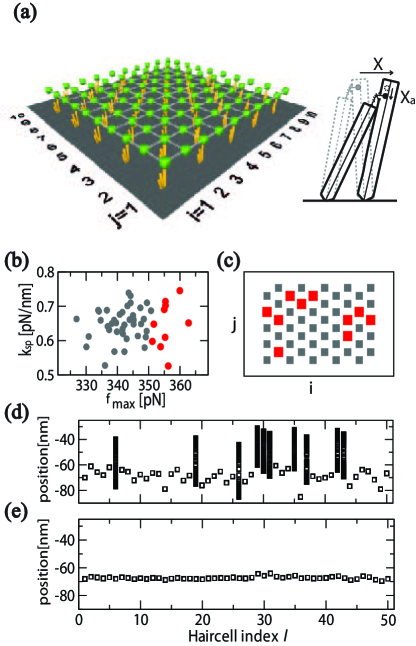
Figure 1: (a) Schematic figure for the elastically coupled hair bundles with mechanical loading and a schematic figure for a free-standing hair bundle. (b) An example of the parameter distribution. The symbols in red denote the parameters for the hair bundles which have spontaneous oscillating motion in their free-standing states. (c) Spatial distribution of the spontaneously moving hair bundles (red) and quiescent bundles (grey). (d) The stroboscopic view (snap shots at every 0.5 sec for 100 seconds) of 50 uncoupled hair bundles ($k=0$). Each hair cell is numbered using hair cell index $l$. The position of the oscillating hair bundles are spread out as their centre frequency of their motion is about 5 Hz. (e) The stroboscopic view of amplitude death state ($k=2$ pN/nm), which shows the cessation of the spontaneous oscillation shown in (d). Parameters used are listed in Table 1.

The amplitude death region in the presence of thermal noise shows, instead of perfect quenching, suppressed fluctuations of mechanical motions (see Fig. 2(a)). We performed numerical simulations using 17 sets of the parameters with the same mean values and variances. Even though we show only four of them in Fig. 2 (a) for better visibility of the figure, we found amplitude death in all cases (see electronic supplementary material, Fig. S8). To examine the occurrence of the amplitude death, it proves useful to plot the positional variance $\delta X$ instead of its Fourier component, because the spontaneous motion is not very sinusoidal. As inter-bundle coupling strength increases, the positional variance $\delta X$ increases rapidly due to synchronized spontaneous movement. It decreases later due to the amplitude death. The amplitude death arises around k=1$pN/nm$ (See also Fig. S8). This cross-over value for the amplitude death is not universal, but it depends on the distribution of the parameters, the membrane mass or the noise correlation time. We find the cross-over to the amplitude death region arises at weaker coupling strength for shorter thermal correlation time $\tau_{c}$ (see Fig. S5 (a)).

3.2 Response of open channel probability to external stimulus

Let us consider the neural response of the hair bundles in the amplitude death state. The influx of cations through the transduction channels depolarizes the cell membrane which opens voltage-gated channels at the base of the hair cell and generates a synaptic current[22]. The information on the auditory stimulus is passed along the auditory nerve in the form of a spike train. Simplifying the process, we assume the neuron spike rate is proportional to transduction current[23]. Then, concerning the spike rates of a bundle of the neurons, rather than the averaged displacement of hair bundles, it is more appropriate to consider an averaged open probability,

$$P^{*}_{o}=\frac{1}{N_{c}}\sum_{l=1}^{N_{c}}P_{o,l},$$ (5)

where $N_{c}$ is the number of hair cells.

In Figs. 2 (b), (c), and (d), we plot $P^{*}_{o}(t)$ when a pure tone stimulus at the frequency 6 Hz is applied when 40 s < time < 60 s. Compared to the case of uncoupled hair bundles (Fig. 2(b)), the weakly coupled hair bundles (Fig. 2(c)) show a strong amplification of the signal in the open probability $P^{*}_{o}$. But this signal amplification appears together with unwanted strong noise (see the data in the absence of the signal in Fig. 2(c) when time < 40 s, time> 60 s). The noisy fluctuation of the open channel probability limits the threshold of the auditory signal, because the acoustic signal drowned in the $P_{0}^{*}$ fluctuation cannot be encoded in the neuronal signal. The amplitude death resolves this problem. It suppresses intrinsic noise which may exceed the input signal (see Fig. 2(d)). It is interesting to note that the background noise of the open probability is much weaker in the amplitude death state (Fig. 2 (d)) than in the uncoupled system (Fig. 2 (b)).

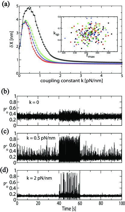
Figure 2: (a) The positional variance $\delta X\equiv\sqrt{\overline{X^{2}}-\overline{X}^{2}}$ of the averaged displacement $X=\frac{1}{N_{c}}\sum_{l}X_{l}$ over hair cells where $\overline{\cdots}$ means time-average, which shows suppression of the mechanical fluctuation of hair bundles as the inter-bundle coupling strength increases. The initial $\delta X$ increase is due to the synchronization of the hair bundle movement. Each color denotes the result for each set of parameters which is shown in the inset. The response of the averaged open probability $P^{*}_{o}(t)$ to a 6 Hz stimulus $F(t)=\sin(6\times 2\pi\frac{\rm time}{\rm sec})$ pN for 40 s < time < 60 s (otherwise $F(t)$=0) is shown (b) when the hair bundles are uncoupled ($k=0$), (c) when the hair bundles show a coherent spontaneous motion ($k=0.5$ pN/nm), and (d) when the hair bundles are in the amplitude death region ($k=2$ pN/nm). In the amplitude death state (d), the spontaneous fluctuation in (c) is strongly suppressed but still the response is significantly stronger than the uncoupled case in (b). Parameters used are listed in Table 1.

3.3 Signal-to-noise ratio

The sources of noise can be divided into those which arise from (i) fluctuation associated with an active force generated by hair bundles, (ii) thermal fluctuation associated with the Browninan motion of hair bundles, and (iii) fluctuation associated with the stochastic nature of channel opening. Source (i) appears to dominate at weak couplings where the bundles are free-standing or showing collective spontaneous motion. Source (ii) is the main source of noise in the amplitude death region where the hair bundles’ spontaneous movements are suppressed.

The hair bundles’ active forces magnify the mechanical response of the oscillatory stimulus, but this amplification also enhances the background noise. To investigate the competition between the signal amplification and the noise reduction, we calculate the power spectra of mechanical displacement,

$$\tilde{S}_{X}(\omega)=\frac{1}{N_{c}}\sum_{l=1}^{N_{c}}|\tilde{X}_{l}(\omega)|^{2},\leavevmode\nobreak\ \leavevmode\nobreak\ \tilde{X}_{l}(\omega)=\frac{1}{T_{a}}\int_{0}^{T_{a}}X_{l}(t)e^{i\omega t}dt,$$ (6)

where $T_{a}$ is the time period for the Fourier transformation and $\omega=2\pi f$ is the angular frequency. We plot $\tilde{S}_{X}(\omega)$ for $f=$6 Hz pure tone signal of the amplitude 0.05 pN (Fig. 3 (a), (b), and (c)) and 0.5 pN (Fig. 3 (d), (e), and (f)). When a weak acoustic signal is applied to uncoupled hair bundles, the signal can be drowned in the power spectrum as shown in Fig. 3 (a). While one can see an amplified signal by weakly coupled hair bundles in Fig. 3 (b), the intrinsic noise is also strong and the single tone signal at 6 Hz is vaguely seen ( see green arrow in Fig. 3 (b)). In contrast to these cases, the input acoustic signal can be clearly seen in the amplitude death region (Fig. 3 (c)) where the background noise level is severely reduced by about two orders of magnitude.

For the signal with sufficient strengths (Fig. 3 (d), (e), and (f)), the amplification of the oscillatory stimulus is more prominent than the background noise reduction. For the signal with the amplitude of $F=0.5$ pN, the power spectra of coupled hair bundles in Fig. 3(e) and (f) show the second harmonic at $2f=$12 Hz due to the nonlinearity. This is in contrast to the case of uncoupled hair bundles (Fig. 3 (d)) which does not show the harmonics. When a weak signal is applied to the system in the amplitude death region, noise reduction (rather than signal amplification) more significantly contributes to the enhancement of the signal transmission ( Fig. 3 (a), (b), and (c)). Provided the neuronal threshold is low enough, the amplitude death phenomenon allows the auditory systems to have a low threshold of acoustic stimulus.

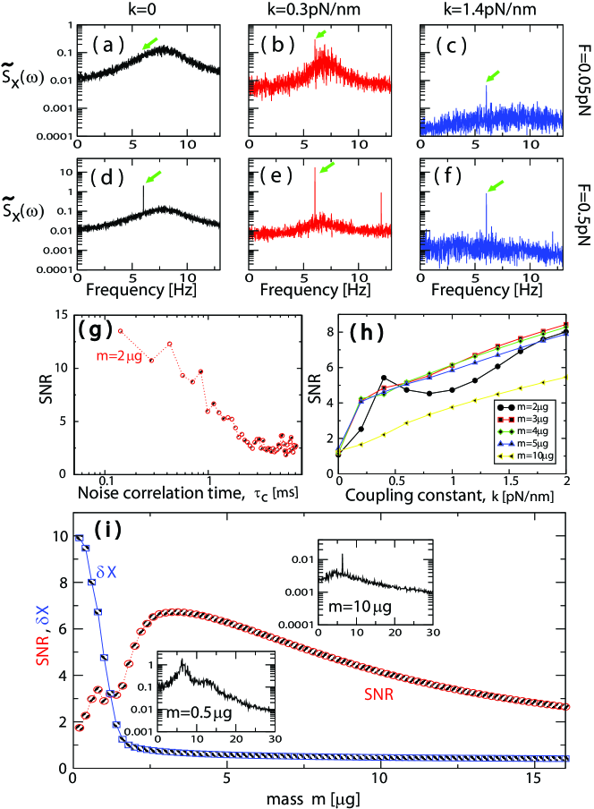
Figure 3: The power spectra of mechanical displacement $\tilde{S}_{X}(\omega)$ as a function of frequency $f=\omega/2\pi$ when a 6 Hz stimulus is applied with amplitude of $F$=0.05 pN ((a),(b),(c)) and $F$= 0.5 pN ((d),(e),(f)). The coupling strengths are ((a),(d)) $k$=0, ((b),(e)) $k$=0.3 pN/nm, ((c),(f)) $k$=1.4 pN/nm. The time period for Fourier transformation $T_{a}$ is 100s. Note that the remarkable change in the noise floor level in the figures from (a) to (f). A second harmonic at 12 Hz appears in (e) and (f). (g) SNR as a function of the correlation time $\tau_{c}$ for $k=$1.2 pN/nm. (h) SNR as a function of the coupling strength $k$ for the various masses and $\tau_{c}$=1.4 ms. (i) SNR and $\delta X$ as a function of the mass $m$ for $\tau_{c}=1.4$ ms and $k=$1.2 pN/nm, which shows that SNR has maximum value at $m=3\mu$g in the amplitude death region. The inset shows the power spectra for different mass $m$. For the simulation from (g) to (i), $F=0.1$ pN. We used the averaged power spectra over ten different trials of thermal noise force. Parameters used are listed in Table 1.

Signal-to-noise ratio (SNR) is a measure that compares the level of a desired signal to the level of background noise. It is defined by

$$SNR=\lim_{\Delta\omega\rightarrow 0}\frac{\tilde{S}_{X}(\Omega)}{\frac{1}{\Delta\omega}\int_{\Omega-\Delta\omega/2}^{\Omega+\Delta\omega/2}\tilde{S}_{X}(\omega)d\omega},$$ (7)

where $\Omega$ is the angular frequency of the oscillatory stimulus; $F(t)=F\sin\Omega t$ in Eq. (2.1). In Fig. 3 (g),(h), and (i), we plot the SNR for various parameters. We find the SNR increases steadily as we decrease the noise correlation time (Fig. 3 (g)). Since the noise strength and the bandwidth of the thermal noise is inversely proportional to the correlation time, our finding indicates a positive role of noise in the sense that the SNR increases with the noise strength. However, the physical origin of this phenomenon must be different from the orthodox theory of stochastic resonance[24], because we observed SNR is simply decreased by a fictitious increase of the noise strength at a fixed correlation time.

3.4 Optimal loading for SNR and amplitude death

Our simulation of the system shows that the SNR has approximately monotonic dependence on elastic coupling strength $k$ (Fig. 3 (h)). Meanwhile, we find SNR has non-monotonic dependence on the mass of the overlying membrane (Fig. 3(i)). We find that there exists an optimal value of the mass which maximizes SNR. This is a result of the competition between active amplification and noise reduction. The force signal to a hair bundle is more amplified (accelerated) for lighter masses but the hair bundle’s motion also becomes more noisy. This noisy motion is suppressed by the inter-bundle coupling and we find that the maximal SNR arises when the hair bundles are in the amplitude death region. Fig. 3(i) shows when SNR reaches its peak value at $m=3\mu$g, the positional variance $\delta X$ is already minimal. Therefore, we conclude that the active hair bundles of a bullfrog’s sacculus may rely on the amplitude death mechanism to enhance signal transmission.

There has been a long-standing problem on the anomalously low threshold of acoustic stimulus in hair bundles[25]. If the individual hair bundle is described by a mass $m$ on a spring of stiffness $\kappa$, its positional fluctuation in thermal equilibrium is $\delta x=\sqrt{k_{B}T/\kappa}$ according to the equipartition theorem. Thus, theoretical $\delta x$ is larger than 2 nm because in no inner-ear organ has the bundle stiffness been found to exceed $\kappa\sim 1$ pN/nm[25]. But many experimental data suggest that the displacement of smaller than 0.1 nm is readily detectable ( see Bialek[25] and references therein). We think that the amplitude death may provide a key to this problem. In the amplitude death region, the positional fluctuations of coupled hair bundles are strongly suppressed, so that $\delta x$ can be as small as 0.1 nm in spite of thermal noise. In this region, the hair bundles can detect even $F\sim 0.05$ pN where the signal is clearly visible compared to background noise level (Fig. 3(c)). This signal would be completely drowned out if they were uncoupled (Fig. 3(a)). Assuming $F\sim 0.05$ pN is the minimum detectable stimulus, we can estimate the mass per hair bundle as $m\approx 0.05{\rm pN}/a_{\rm th}$ where $a_{\rm th}$ is the smallest detectable peak acceleration of vibration. Lewis et al.[6] reported that a frog’s sacculus can detect the acceleration down to $a_{\rm th}\sim 10^{-6}g\sim 10^{-5}{\rm m/s^{2}}$. From this value, we estimate $m\approx 5\mu$g which is not significantly different from the mass causing the maximal SNR in Fig. 3(h). This estimation leads us to reason that the anomalously low stimulus threshold $\delta x\sim$ 0.1 nm might be achieved through the amplitude death mechanism, which is difficult to be detected by an individual hair bundle[8].

3.5 Frequency selectivity

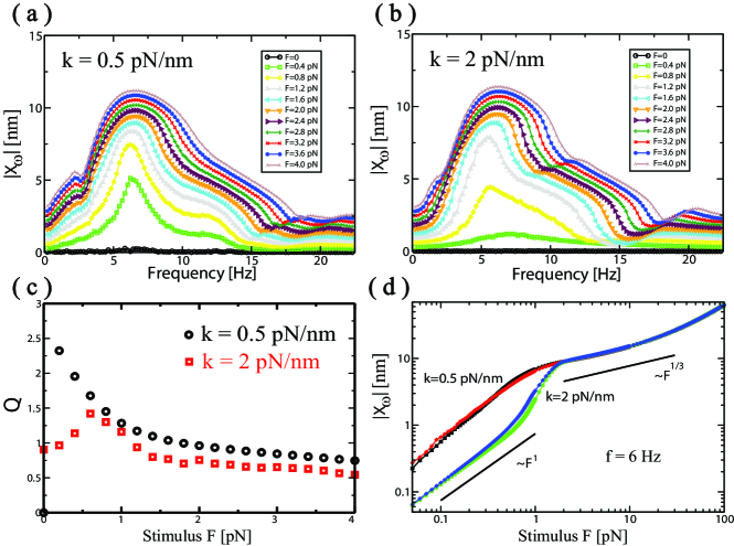
Figure 4: (a) The response of the Fourier component of mechanical displacement $|X_{\omega}|$= $|\frac{1}{N_{c}}\sum_{l}\tilde{X}_{l}(\omega)|$ as a function of the frequency $f=\omega/2\pi$ for the system in the spontaneous oscillating region ($k=0.5$ pN/nm). (b) The same plot for the amplitude death region ($k=2$ pN/nm). (c) The quality factor Q vs. the stimulus strength F. The quality factor of the coupled bundles is lower in the amplitude death state and weakly dependent on the stimulus strength. (d) $|X_{\omega}|$ as a function of the stimulus amplitude $F$ for two different coupling strengths and two different sets of the hair-bundle-distribution parameters (denoted by different colors). It shows the linear response for the weak stimulus. Beyond this region, the response roughly shows a $1/3$ law where the responses for two different coupling strengths coincide. Parameters used are listed in Table 1.

In Fig. 4 (a) and (b), we plot the mechanical response of the hair bundles $|X(\omega)|=|\frac{1}{N_{c}}\sum_{l}\tilde{X}_{l}(\omega)|$ for the stimulus of the frequency $f=\omega/2\pi$. The spontaneous oscillating region (Fig. 4(a)) shows slightly better frequency selectivity than the amplitude death region (Fig. 4(b)) only for weak enough stimuli ($F\leq 0.8$ pN). For the stimuli with $F>$ 0.8 pN, the broadening of the response spectra in both regions is similar. There is no significant difference in the frequency selectivity between the two regions because of the inhomogeneous distribution of hair bundles. The inhomogeneity in our calculation was sufficient to prevent the hair bundles from locking to a single-frequency mode. The frequency selectivity is quantified in terms of height $|X_{\omega_{0}}|$ of the spectral peak at its characteristic angular frequency $\omega_{0}$, and its quality factor Q=$\omega_{0}/|\omega_{2}-\omega_{1}|$ where the halfwidth $|\omega_{2}-\omega_{1}|$ is defined by $|X_{\omega_{1}}|=|X_{\omega_{2}}|=|X_{\omega_{0}}|/2$. Our numerical results for coupled hair bundles of a frog’s sacculus show Q $\sim 1$ (see Fig. 4 (c)). This is consistent with electrophysiological recordings from frog auditory nerve fibers which indicate a high sensitivity to small stimuli ($\sim$ 0.1 nm) but poor frequency selectivity (Q < 1)[4, 5]. A recent experiment[12] even reports the absence of the frequency tuning in frog sacculi when hair bundles are coupled to an overlying membrane. The complete disappearance of the frequency selectivity in Strimbu et al.[12], however, is probably caused by the heavier weight of the artificial membrane in the experiment. In our calculations, as we increase the membrane mass, we observe the peak frequency is lowered and eventually the frequency selectivity disappears (see electronic supplementary material, Fig. S4).

3.6 Comparison to existing models and experiments

Our theory as well as the lower frequency selectivity in experiments[4, 5, 12] are in contrast to the theoretical prediction in Dierkes et al.[26]. The coupled hair bundle model[26] shows sharp frequency selectivity but amplitude death did not appear in the model. We think one of the reasons for the discrepancy is that their non-uniformity was not sufficient to cause amplitude death. It might also be useful to note that when characteristic frequencies are similar, coupling oscillatory and quiescent hair bundles can cause amplitude death more efficiently.

Eguíluz et. al.[27] and Camalet et. al.[23] proposed a generic model which might underlie the essential nonlinearity[28], where hair cells are assumed to operate at the critical point of Hopf bifurcation[9]. According to the critical oscillator model[27, 23], the amplitude response of hair bundles to an oscillatory stimulus with strength $F$ scales as $\sim F^{1/3}$ for arbitrarily weak signals. In our model, the hair cell bundles in the amplitude death region show a linear response at weak stimuli. The response evolves to the region where it shows compressive rates close to a 1/3 law (see Fig. 4(d)). The crossover of the growth from linear to 1/3 nonlinear rates in Fig. 4(d) is consistent with the analytic formula derived from the generic mathematical model of amplitude death (see electronic supplementary material). The hair-bundle nonlinearity shown here is similar to what has been consistently observed in experiments on mammalian cochlea after Rhode[28], where the transition between linear and compressive nonlinear growth has been reported[29, 30, 31]. Our theory is not incompatible with the theory[23, 13] of individual hair bundles. As in Nadrowski et al.[13], our individual hair bundles are assumed to be near the Hopf bifurcation critical point. They were randomly distributed near the critical point with a small width of the distribution.

Stochastic resonance is a phenomenon where SNR is maximized in the presence of a specific non-zero level noise. This phenomenon widely occurs in threshold systems, such as a two-state system separated by an energy barrier. It has been speculated that in the case of free-standing hair bundles (such as inner hair cell bundles), the noise plays a role in acoustic signal processing, by enhancing the sensitivity of the system through stochastic resonance[32]. While it has been reported that applying noise to sacculi may enhance the SNR[33], it is difficult to judge whether the sensation is indeed improved by stochastic resonance. One of the reasons is that the generic stochastic resonance model is not applicable to a coupled system with active dynamics. Instead we ask whether the noise plays any positive role in signal transmission. We find out that the direct increase of the noise strength (e.g. by increasing temperature) at a fixed $\tau_{c}$ simply decreases the SNR. In this sense, the orthodox stochastic resonance phenomenon does not occur in the system. Meanwhile, we may say that the noise can have a positive role in signal transmission, in the sense that the thermal noise enhances the SNR by suppressing the spontaneous activity of hair bundles. To explain the process, we need to mention that there are two different types of apparently similar hair bundles moving in the presence of noise. The first type spontaneously oscillates regardless of noise. The second type is quiescent in the absence of the noise, but they are in motion in the presence of noise. As the thermal correlation time becomes shorter, the motion of the second type of hair bundles vanishes, thereby enhancing the SNR (see electronic supplementary material, Fig. S3 (a)).

Barral et al.[34] performed experiments on a hair bundle of the bullfrog sacculus which is coupled to simulated ’cyber’ bundles. They argue that the coupling increases the phase coherence between hair bundles, which endows the hair bundles with better characteristics. This is in contrast to our suggestion that the cessation of the oscillation has useful properties. We think the discrepancy between the two is a question of the strength of the coupling and the inhomogeneity of the bundles. Barral et al[34] went up to around 0.5 pN/nm stiffness, where we expect they could also observe amplitude death if they would increase the coupling stiffness. Regarding the coupling strength, how strong is strong enough for the amplitude death phenomenon depends on the inhomogeneity of hair bundles (see electronic supplementary material). We believe, if the two bundles are sufficiently different (for instance one is quiescent and the other is oscillating) then the experiments of the type in Barral et al[34] can show amplitude death even for the coupling of 0.5 pN/nm stiffness.

4 Conclusion

Using numerical simulations, we have demonstrated that a signal amplification and noise reduction in coupled hair bundles can appear through amplitude death. The signal-to-noise ratio can be maximized when the coupled hair bundles are in the amplitude death state. While individual hair bundles in a frog’s sacculus show spontaneous oscillation, we think this oscillation in vivo is suppressed to obtain high signal-to-noise ratio. Our finding is consistent with the recent experimental observation[11] showing the absence of the spontaneous oscillations when they are coupled with an overlying membrane.

When individual systems are coupled, the net system is often described as coupled individual systems or sometimes is considered as one new system. In which class, do our hair bundles in the amplitude death region belong to? The minimum inter-bundle coupling strengths for the amplitude death in most of our calculations were comparable to the intrinsic stiffness of hair bundles ($k_{\rm sp}=$0.65 pN/nm). Since the amplitude death phenomenon can arise even when the inter-bundle coupling is weaker than the intrinsic stiffness, we think that the hair bundles in amplitude death region can be considered as weakly coupled independent oscillators although more quantitative analysis is necessary to clarify this issue.

The transduction mechanism presented in this work can be used to fabricate low-noise amplification in acoustic sensors. A cantilever-type mechanical sensor can act similar to hair cell bundle when it has biomimetic feedback action[35, 36]. The amplitude death phenomenon in a coupled array of these biomimetic sensors will lead to a low-noise amplification with an enhanced signal-to-noise ratio.

This work was supported by Basic Science Research Program through the National Research Foundation of Korea (NRF) funded by the MEST (2011-0009557). The author thanks Marie Curie Fellowship (2010-2011) of EU through University of Bath in UK.

Figure Captions

Fig. 1 (a) Schematic figure for the elastically coupled hair bundles with mechanical loading and a schematic figure for a free-standing hair bundle. (b) An example of the parameter distribution. The symbols in red denote the parameters for the hair bundles which have spontaneous oscillating motion in their free-standing states. (c) Spatial distribution of the spontaneously moving hair bundles (red) and quiescent bundles (grey). (d) The stroboscopic view (snap shots at every 0.5 sec for 100 seconds) of 50 uncoupled hair bundles ($k=0$). Each hair cell is numbered using hair cell index $l$. The position of the oscillating hair bundles are spread out as their centre frequency of their motion is about 5 Hz. (e) The stroboscopic view of amplitude death state ($k=2$ pN/nm), which shows the cessation of the spontaneous oscillation shown in (d). Parameters used are listed in Table 1.

Fig. 2 (a) The positional variance $\delta X\equiv\sqrt{\overline{X^{2}}-\overline{X}^{2}}$ of the averaged displacement $X=\frac{1}{N_{c}}\sum_{l}X_{l}$ over hair cells where $\overline{\cdots}$ means time-average, which shows suppression of the mechanical fluctuation of hair bundles as the inter-bundle coupling strength increases. The initial $\delta X$ increase is due to the synchronization of the hair bundle movement. Each color denotes the result for each set of parameters which is shown in the inset. The response of the averaged open probability $P^{*}_{o}(t)$ to a 6 Hz stimulus $F(t)=\sin(6\times 2\pi\frac{\rm time}{\rm sec})$ pN for 40 s < time < 60 s (otherwise $F(t)$=0) is shown (b) when the hair bundles are uncoupled ($k=0$), (c) when the hair bundles show a coherent spontaneous motion ($k=0.5$ pN/nm), and (d) when the hair bundles are in the amplitude death region ($k=2$ pN/nm). In the amplitude death state (d), the spontaneous fluctuation in (c) is strongly suppressed but still the response is significantly stronger than the uncoupled case in (b). Parameters used are listed in Table 1.

Fig. 3 The power spectra of mechanical displacement $\tilde{S}_{X}(\omega)$ as a function of frequency $f=\omega/2\pi$ when a 6 Hz stimulus is applied with amplitude of $F$=0.05 pN ((a),(b),(c)) and $F$= 0.5 pN ((d),(e),(f)). The coupling strengths are ((a),(d)) $k$=0, ((b),(e)) $k$=0.3 pN/nm, ((c),(f)) $k$=1.4 pN/nm. The time period for Fourier transformation $T_{a}$ is 100s. Note that the remarkable change in the noise floor level in the figures from (a) to (f). A second harmonic at 12 Hz appears in (e) and (f). (g) SNR as a function of the correlation time $\tau_{c}$ for $k=$1.2 pN/nm. (h) SNR as a function of the coupling strength $k$ for the various masses and $\tau_{c}$=1.4 ms. (i) SNR and $\delta X$ as a function of the mass $m$ for $\tau_{c}=1.4$ ms and $k=$1.2 pN/nm, which shows that SNR has maximum value at $m=3\mu$g in the amplitude death region. The inset shows the power spectra for different mass $m$. For the simulation from (g) to (i), $F=0.1$ pN. We used the averaged power spectra over ten different trials of thermal noise force. Parameters used are listed in Table 1.

Fig. 4 (a) The response of the Fourier component of mechanical displacement $|X_{\omega}|$= $|\frac{1}{N_{c}}\sum_{l}\tilde{X}_{l}(\omega)|$ as a function of the frequency $f=\omega/2\pi$ for the system in the spontaneous oscillating region ($k=0.5$ pN/nm). (b) The same plot for the amplitude death region ($k=2$ pN/nm). (c) The quality factor Q vs. the stimulus strength F. The quality factor of the coupled bundles is lower in the amplitude death state and weakly dependent on the stimulus strength. (d) $|X_{\omega}|$ as a function of the stimulus amplitude $F$ for two different coupling strengths and two different sets of the hair-bundle-distribution parameters (denoted by different colors). It shows the linear response for the weak stimulus. Beyond this region, the response roughly shows a $1/3$ law where the responses for two different coupling strengths coincide. Parameters used are listed in Table 1.

References

- [1] Crawford AC, Fettiplace R. 1985 The mechanical properties of ciliary bundles of turtle cochlear hair cells. J. Physiol. 364, 359-379.
- [2] Howard J, Hudspeth AJ. 1987 Mechanical relaxation of the hair bundle mediates adaptation in mechanoelectrical transduction by the bullfrog’s saccular hair cell. Proc. Natl. Acad. Sci. U.S.A. 84, 3064-3068.
- [3] Ashmore J. 2008 Cochlear outer hair cell motility. Physiol. Rev. 88(1),173-210.(doi:10.1152/physrev.00044.2006)
- [4] Narins PM, Lewis ER. 1984 The vertebrate ear as an exquisite seismic sensor. The Journal of the Acoustical Society of America 76, 1384-1387. (doi: 10.1121/1.391455)
- [5] Lewis ER. 1988 Tuning in the bullfrog ear. Biophys. J. 53, 441-447. (doi: 10.1016/S0006-3495(88)83120-5)
- [6] Lewis ER, Narins PM, Cortopassi KA, Yamada WM, Poinar EH, Moore SW, and Yu XL. 2001 Do male white-lipped frogs use seismic signals for intraspecific communication? Amer. Zool. 41, 1185-1199. (doi: 10.1093/icb/41.5.1185)
- [7] Martin P, Bozovic D, Choe Y, Hudspeth AJ. 2003 Spontaneous Oscillation by Hair bundles of the Bullfrog’s Sacculus The Journal of Neuroscience 23(11), 4533-4548.
- [8] Martin P, Mehta AD, Hudspeth AJ. 2000 Negative hair-bundle stiffness betrays a mechanism for mechanical amplification by the hair cell. Proc. Natl. Acad. Sci. U.S.A. 97, 12026-12031.(doi: 10.1073/pnas.210389497 )
- [9] Strogatz SH. 1994 Nonlinear Dynamics And Chaos: With Applications To Physics, Biology, Chemistry, And Engineering, Addison Wesley Publishing Company.
- [10] Pikovsky A, Rosenblum M, Kurths J. 2001 Synchronization: A universal concept in nonlinear sciences, Cambridge University Press, Cambridge.
- [11] Strimbu CE, Kao A, Tokuda J, Ramunno-Johnson D, Bozovic D. 2010 Dynamic state and evoked motility in coupled hair bundles of the bullfrog sacculus. Hear. Res. 265 38-45. (doi: 10.1016/j.heares.2010.03.001)
- [12] Strimbu CE, Fredrikson-Hemsing L, Bozovic D. 2012 Coupling and elastic loading affects the active response by the inner ear hair cell bundles. PLoS ONE 7, e33862 1-9. (doi:10.1371/journal.pone.0033862)
- [13] Nadrowski B, Martin P, Jülicher F. 2004 Active hair-bundle motility harnesses noise to operate near an optimum of mechanosensitivity. Proc. Natl. Acad. Sci. U.S.A. 101, 12195-12200. (doi: 10.1073/pnas.0403020101)
- [14] Aronson DG, Ermentrout GB, Kopell N. 1990 Amplitude response of coupled oscillators, Physica D 41, 403-449. (doi:10.1016/0167-2789(90)90007-C)
- [15] Rayleigh JWS. 1945 The Theory of Sound, Dover Publications, New York, NY, USA.
- [16] Ryu JW, Lee DS, Park YJ, Kim CM. 2009 Oscillation Quenching in Coupled Different Oscillators. Journal of the Korean Physical Society 55, 395-399.
- [17] Smotherman MS, Narins PM. 2000 Hair cells, Hearing and Hopping: A Field Guide to Hair Cell Physiology in the Frog. The Journal of Expermental Biology 203, 2237-2246.
- [18] Ramunno-Johnson D, Strimbu CE, Fredrickson L, Arisaka K, Bozovic D. 2009 Distribution of frequencies of spontaneous oscillations in hair cells of the bullfrog sacculus. Biophysical Journal 96, 1159-1168. (doi:10.1016/j.bpj.2008.09.060)
- [19] Press WH, Teukolsky SA, Vetterling WT, Flannery BP. 1992 Numerical Recipes in Fortran 77, Cambridge University Press.
- [20] Ramana Reddy DV, Sen A, Johnston GL. 1998 Time delay induced death in coupled limit cycle oscillators. Phys. Rev. Lett. 80, 5109-5112. (doi: 10.1103/PhysRevLett.80.5109)
- [21] Prasad A, Dhamala M, Adhikari BM, Ramaswamy R. 2010 Amplitude death in nonlinear oscillators with nonlinear coupling. Phys. Rev. E 81, 027201- 1–4. (doi: 10.1103/PhysRevE.81.027201)
- [22] Hudspeth AJ. 1989 How the ear’s works work. Nature 341, 397-404.
- [23] Camalet S, Duke T, Jülicher F, Prost J. 2000 Auditory sensitivity provided by self-tuned critical oscillations of hair cells. Proc. Natl. Acad. Sci. U.S.A. 97, 3183-3188.(doi: 10.1073/pnas.97.7.3183)
- [24] Gammaitoni L, Hänggi P, Jung P, Marchesoni F. 1998 Stochastic Resonance. Review of Modern Physics 70, 223–287. (doi:10.1103/RevModPhys.70.223)
- [25] Bialek W. 1987 Physical limits to sensation and perception. Ann. Rev. Biophys.Biophys. Chem. 16, 455-478. (doi:10.1146/annurev.bb.16.060187.002323)
- [26] Dierkes K, Lindner B, Jülicher F. 2008 Enhancement of sensitivity gain and frequency tuning by coupling of active hair bundles. Proc. Natl. Acad. Sci. U.S.A. bf 105, 18669-18674. (doi: 10.1073/pnas.0805752105)
- [27] Eguíluz VM, Ospeck M, Choe Y, Hudspeth AJ, Magnasco MO. 2000 Essential nonlinearity in hearing. Phys. Rev. Lett. 84, 5232-5235. (doi: 10.1103/PhysRevLett.84.5232)
- [28] Rhode WS. 1971 Observations of the vibration of the basilar membrane in squirrel monkeys using the Mössbauer technique. J. Acoust. Soc. Am. 49, 1218-1231. (doi: 10.1121/1.1912485)
- [29] Ruggero MA, Rich NC, Recio A, Narayan SS, Robles L. 1997 Basilar-membrane responses to tones at the base of the chinchilla cochlea. J. Acoust. Soc. Am. 101, 2151-2163. (doi:10.1121/1.418265)
- [30] Ruggero MA, Narayan SS, Temchin AN, Recio A. 2000 Mechanical bases of frequency tuning and neural excitation at the base of the cochlea: Comparison of basilar-membrane vibrations and auditorynerve- fiber responses in chinchilla. Proc. Natl. Acad. Sci. U.S.A. 97, 11744-11750. (doi: 10.1073/pnas.97.22.11744)
- [31] Nuttal AL, Dolan DF. 1996 Steady-state sinusoidal velocity responses of the basilar membrane in guinea pig. J. Acous. Soc. Am. 93, 1556-1565. (doi:10.1121/1.414732)
- [32] Jaramillo F, Wiesenfeld K. 1998 Mechanoelectrical transduction assisted by Brownian motion: a role for noise in the auditry system. Nature Neurosci. 1, 384-388. (doi:10.1038/1597)
- [33] Indresano AA, Frank JE, Middleton P, Jaramillo F. 2003 Mechanical noise enhances signal transmission in the bullfrog sacculus. J. Assoc. Res. Otolarygol. 4(3), 363-370. (doi:10.1007/s10162-002-3044-4)
- [34] Barral J, Dierkes K, Lindner B, Martin P, 2010 Coupling a sensory hair-cell bundle to cyber clones enhances nonlinear amplification. Proc. Natl. Acad. Sci. U.S.A. 107, 8079-8084.(doi/10.1073/pnas.0913657107)
- [35] Kim H, Song T, Ahn KH. 2011 Sharply tuned small force measurement with a biomimetic sensor. Appl. Phys. Lett. 98, 013704. (doi:10.1063/1.3533907)
- [36] Song T, Park HC, Ahn KH. 2009 Proposal for high sensitivity force sensor inspired by auditory hair cell. Appl. Phys. Lett. 95, 013702. (doi: 10.1063/1.3167818)
- [37] Hacohen N, Assad JA, Smith WJ, Corey DP. 1989 J. Neurosci. 9, 3988-3997.
- [38] Jacobs RA, Hudspeth AJ. 1990 Cold Spring Harbor Symp. Quant. Biol. 55, 547-561.