Mean Field Bayes Backpropagation: scalable training of multilayer neural networks with binary weights

Abstract

Significant success has been reported recently ucsing deep neural networks for classification. Such large networks can be computationally intensive, even after training is over. Implementing these trained networks in hardware chips with a limited precision of synaptic weights may improve their speed and energy efficiency by several orders of magnitude, thus enabling their integration into small and low-power electronic devices. With this motivation, we develop a computationally efficient learning algorithm for multilayer neural networks with binary weights, assuming all the hidden neurons have a fan-out of one. This algorithm, derived within a Bayesian probabilistic online setting, is shown to work well for both synthetic and real-world problems, performing comparably to algorithms with real-valued weights, while retaining computational tractability.

Department of Electrical Engineering, Technion 32000, Haifa, Israel
*Corresponding author: daniel.soudry@gmail.com

1 Introduction

Recently, Multilayer Neural Networks (MNNs) with deep architecture have achieved state-of-the-art performance in various machine learning tasks (Hinton et al., 2012; Krizhevsky et al., 2012; Dahl et al., 2012) - even when only supervised on-line gradient descent algorithms are used (Dean et al., 2012; Ciresan et al., 2012a, b). However, it is not clear what would be the best choice of a training algorithm for such networks (Le et al., 2011). Within a Bayesian setting, given some prior distribution and error function, we can choose an on-line optimal estimate based on updating the posterior distribution. Such a “Bayesian” approach has relatively transparent assumptions and, furthermore, gives estimates of learning uncertainty and allows model averaging. However, an exact Bayesian computation is generally intractable. Bayesian approaches, based on Monte Carlo simulations, were previously used (MacKay, 1992; Neal, 1995), but these are not generally scalable with the size of the network and training data. Other approximate Bayesian approaches were suggested (Opper & Winther, 1996; Winther et al., 1997; Opper & Winther, 1998; Solla & Winther, 1998), but only for Single-layer Neural Networks (SNN). To the best of our knowledge, it is still unknown whether such methods could be generalized to multilayer networks.

Another advantage for a Bayesian approach is that it can be used even when gradients do not exist. For example, it could be very useful if weights are restricted to assume only binary values (e.g., $\pm 1$). This may allow a dense, fast and energetically efficient hardware implementation of MNNs (e.g., with the chip in (Karakiewicz et al., 2012), which can perform $10^{12}$ operations per second with $1\mathrm{mW}$ power efficiency). Limiting the weights to binary values only mildly reduces the (linear) computational capacity of a MNN (at most, by a logarithmic factor (Ji & Psaltis, 1998)). However, learning in a Binary MNN (BMNN - a MNN with binary weights) is much harder than learning in a Real-valued MNN (RMNN - a MNN with real valued weights). For example, if the weights of a single neuron are restricted to binary values, the computational complexity of learning a linearly separable set of patterns becomes NP-hard (instead of P) in the dimension of the input (Fang & Venkatesh, 1996). In spite of this, it is possible to train single binary neurons in a typical linear time (Fang & Venkatesh, 1996). Interestingly, the most efficient methods developed for training single binary neurons use approximate Bayes approaches, either explicitly (Solla & Winther, 1998; Ribeiro & Opper, 2011) or implicitly (Braunstein & Zecchina, 2006; Baldassi et al., 2007).

However, as far as we are aware, it remains an open question whether a BMNN can be trained efficiently by such Bayesian methods, or by any other method. Standard RMNNs are commonly trained in supervised mode using the Backpropagation algorithm (LeCun & Bottou, 1998). However, it is unsuitable if the weight values are binary (crude discretization of the weights is usually quite destructive (Moerland & Fiesler, 1997)). Other, non-Bayesian methods were suggested in the 90’s (e.g., (Saad & Marom, 1990; Battiti & Tecchiolli, 1995; Mayoraz & Aviolat, 1996)) for small BMNNs, but it is not clear whether these approaches are scalable.

In this work we derive a Mean Field Bayes Backpropagation (MFB-BackProp) algorithm for learning synaptic weights in BMNNs where each hidden neuron has only a single outgoing connection (however, the input layer can be fully connected to the first neuronal layer, see Fig. 1). This algorithm has linear computational complexity in the number of weights, similarly to standard Backpropagation. Also, it is parameter-free except for the initial conditions (“prior”). The algorithm implements a Bayes update to the weights, using two approximations (as was done in (Solla & Winther, 1998; Ribeiro & Opper, 2011) for SNNs): (1) a mean-field approximation - the posterior probability of the synaptic weights is approximated by the product of its marginals at each time step, (2) the fan-in of all neurons is large (so their inputs are approximately Gaussian). Despite these approximations, we demonstrate numerically that the algorithm works well. First, we demonstrated its effectiveness in a synthetic teacher-student scenario where the outputs are generated from a network with a known architecture. The network performed well even though the assumption of large fan-in did not hold. We then tested it for a large BMNN ($\sim 10^{6}$ weights) on the standard MNIST task, achieving an error rate comparable with the RMNN of similar size. Therefore, as far as we are aware, it is the first scalable algorithm for BMNNs and the first scalable Bayesian algorithm for MNNs in general (i.e., it does not require Monte Carlo simulations, as in (MacKay, 1992; Neal, 1995)). Hopefully, the methods developed here could lead to scalable hardware implementations, as well as efficient Bayesian-based learning in MNNs.

2 Preliminaries

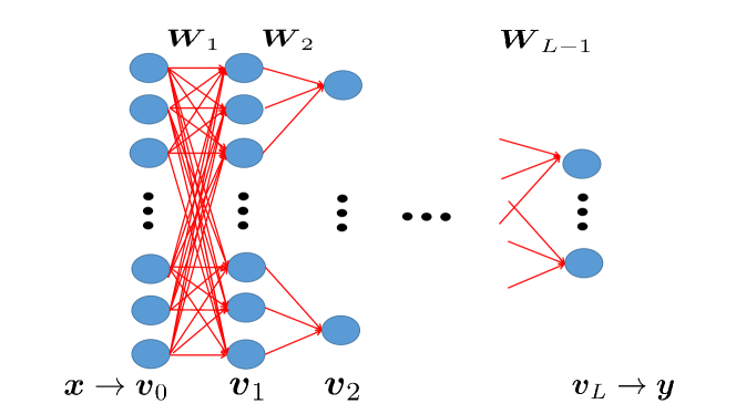
Figure 1: The convergent architecture of the network - all hidden neurons have fan-out 1, while input layer is fully connected.

Notation

We denote by $P\left(x\right)$ the probability distribution (in the discrete case) or density (in the continuous case) of a random variable $X$, $P\left(x|y\right)=P\left(x,y\right)/P\left(y\right)$,$\left\langle x\right\rangle=\int xP\left(x\right)dx$, $\left\langle x|y\right\rangle=\int xP\left(x|y\right)dx$, $\mathrm{Cov}\left(x,y\right)=\left\langle xy\right\rangle-\left\langle x\right\rangle\left\langle y\right\rangle$ and $\mathrm{Var}\left(x\right)=\mathrm{Cov}\left(x,x\right)$. Integration is exchanged with summation in the discrete case. Furthermore, we make use of the following functions: (1) $\theta\left(x\right)$, the Heaviside function (i.e. $\theta\left(x\right)=1$ for $x>0$ and zero otherwise), (2) $\delta_{ij}$, the Kronecker delta function (i.e. $\delta_{ij}=1$ if $i=j$ and zero otherwise). Also, If $\mathbf{x}\sim\mathcal{N}\left(\boldsymbol{\mu},\boldsymbol{\Sigma}\right)$ then it is Gaussian with mean $\boldsymbol{\mu}$ and covariance matrix $\boldsymbol{\Sigma}$, and we denote its density by $\mathcal{N}\left(\mathbf{x}|\boldsymbol{\mu},\boldsymbol{\Sigma}\right)$. Finally, $\Phi\left(x\right)=\int_{-\infty}^{x}\mathcal{N}\left(x|0,1\right)dx$, is the Gaussian cumulative distribution function.

Model

We consider a BMNN with $L$ layers of synaptic weight matrices $\mathcal{W}=\left\{\mathbf{W}_{l}\in\left\{-1,1\right\}^{V_{l}\times V_{l-1}}\right\}_{l=1}^{L}$ connecting neuronal layers sequentially, with $V_{l}$ being the width of the $l$-th layer. We denote the outputs of the layers by $\left\{\mathbf{v}_{l}\right\}_{l=0}^{L}$, where $\mathbf{v}_{0}$ is the input layer, $\left\{\mathbf{v}_{l}=\mathrm{sign}\left(\mathbf{W}_{l}\mathbf{v}_{l-1}\right)\in\left\{-1,1\right\}^{V_{l}}\right\}_{l=1}^{L}$ are the hidden layers (with the $\mathrm{sign}\mathrm{\left(\cdot\right)}$ function operating component-wise) and the $\mathbf{v}_{L}$ is the output layer. The output of the network is therefore

$$\mathbf{v}_{L}=f\left(\mathbf{v}_{0},\mathcal{W}\right)=\mathrm{sign}\left(\mathbf{W}_{L}\mathrm{sign}\left(\mathbf{W}_{L-1}\mathrm{sign}\left(\cdots\mathbf{W}_{1}\mathbf{v}_{0}\right)\right)\right)\,.$$ (1)

Also, we denote $W_{ij,l}=\left(\mathbf{W}_{l}\right)_{ij}$ and $v_{i,l}=\left(\mathbf{v}_{l}\right)_{i}$. Furthermore, we assume the network has a converging architecture, i.e., each hidden neuron has only a single outgoing connection, namely, fan-out$=1$. However, the input layer can be fully connected to the first neuronal layer (Fig. 1). We set $K\left(i,l\right)$ to be the set of indices of neurons in the $\left(l-1\right)$-th layer connected to the $i$-th neuron in the $l$-th layer. For simplicity we assume that $K_{l}=\left|K\left(i,l\right)\right|$ are constant for all $i$. Finally, we denote $i^{\prime}$ to be the index of the neuron in the $\left(l+1\right)$-th layer receiving input from the $i$-th neuron in the $l$-th layer.

Task

We examine a standard supervised learning classification task, in which we are given sequentially labeled data points $D_{N}=\left\{\mathbf{x}^{\left(n\right)},\mathbf{y}^{\left(n\right)}\right\}_{n=1}^{N}$, where $\mathbf{x}^{\left(n\right)}\in\mathbb{R}^{V_{0}}$ is the data point, $\mathbf{y}^{\left(n\right)}\in\left\{-1,1\right\}^{V_{L}}$ is the label and $n$ is the sample index (for brevity, we will sometimes suppress the sample index, where it is clear from the context). As common for supervised learning with MNNs, we assume that $\forall n$ the relation $\mathbf{y}^{\left(n\right)}=f\left(\mathbf{x}^{\left(n\right)},\mathcal{W}\right)$ can be represented by a BMNN with known architecture (the ‘hypothesis class’) and unknown weights $\mathcal{W}$ (i.e, according to Eq. 1 with $\mathbf{v}_{0}=\mathbf{x}^{\left(n\right)}$ and $\mathbf{v}_{L}=\mathbf{y}^{\left(n\right)}$). Our goal is to estimate the weights $\mathcal{W}$.

3 Theory - online Bayesian learning in BMNNs

We approach this task from a Bayesian framework, where we estimate the Maximum A Posteriori (MAP) configuration of weights

$$\mathcal{W}^{*}=\mathrm{argmax}_{\mathcal{W}}P\left(\mathcal{W}|D_{N}\right)\,,$$ (2)

with $P\left(\mathcal{W}|D_{N}\right)$ being the probability for each configuration of the weights $\mathcal{W}$, given the data. We do this in an online setting. Starting with some prior distribution on the weights - $P\left(\mathcal{W}|D_{0}\right)$, we update the value of $P\left(\mathcal{W}|D_{n}\right)$ after the $n$-th sample is received, according to Bayes rule:

$$P\left(\mathcal{W}|D_{n}\right)\propto P\left(\mathbf{y}^{\left(n\right)}|\mathbf{x}^{\left(n\right)},\mathcal{W}\right)P\left(\mathcal{W}|D_{n-1}\right)\,,$$ (3)

for $n=1,\dots,N$. Note that the BMNN is deterministic, so

$$P\left(\mathbf{y}^{\left(n\right)}|\mathbf{x}^{\left(n\right)},\mathcal{W}\right)=\begin{cases}1&,\,\mathrm{if}\,\,\mathbf{y}^{\left(n\right)}=f\left(\mathbf{x}^{\left(n\right)},\mathcal{W}\right)\\ 0&,\,\mathrm{otherwise}\end{cases}\,.$$ (4)

Therefore, the Bayes update in Eq. 3 simply makes sure that $P\left(\mathcal{W}|D_{n}\right)=0$ in any “illegal” configuration (i.e., any $\mathcal{W}^{0}$ such that $\exists k\leq n:\,\mathbf{y}^{\left(k\right)}\neq f\left(\mathbf{x}^{\left(k\right)},\mathcal{W}^{0}\right)$). Unfortunately, this update is generally intractable for large networks, mainly because we need to store and update an exponential number of values for $P\left(\mathcal{W}|D_{n}\right)$. Therefore, some approximation is required.

3.1 Approximation 1: mean-field

Instead of storing $P\left(\mathcal{W}|D_{n}\right)$, we will store its factorized (‘mean-field’) approximation $\hat{P}\left(\mathcal{W}|D_{n}\right)$, for which

$$\hat{P}\left(\mathcal{W}|D_{n}\right)=\prod_{i,j,l}\hat{P}\left(W_{ij,l}|D_{n}\right)\,,$$ (5)

where each factor must be normalized. Notably, it is easy to find the MAP estimate (Eq.  2) under this factorized approximation $\forall i,j,l$

$$W_{ij,l}^{*}=\mathrm{argmax}_{W_{ij,l}\in\left\{-1,1\right\}}\hat{P}\left(W_{ij,l}|D_{N}\right)\,.$$ (6)

The factors $\hat{P}\left(W_{ij,l}|D_{n}\right)$ can be found using a standard variational approach Bishop (2006); Solla & Winther (1998). For each $n$, we first perform the Bayes update in Eq. 3 with $\hat{P}\left(\mathcal{W}|D_{n-1}\right)$ instead of $P\left(\mathcal{W}|D_{n-1}\right)$. Then, we project the resulting posterior onto the family of distributions factorized as in Eq. 5, by minimizing the reverse Kullback-Leibler divergence. A straightforward calculation shows that the optimal factor is just a marginal of the posterior (see supplemental material, section A). Performing this marginalization on the Bayes update and re-arranging terms, we obtain $\forall i,j,l$

$$\hat{P}\left(W_{ij,l}|D_{n}\right) \propto\hat{P}\left(\mathbf{y}^{\left(n\right)}|\mathbf{x}^{\left(n\right)},W_{ij,l},D_{n-1}\right)\hat{P}\left(W_{ij,l}|D_{n-1}\right)\,,$$ (7)

where

$$\hat{P}\left(\mathbf{y}^{\left(n\right)}|\mathbf{x}^{\left(n\right)},W_{ij,l},D_{n-1}\right) = \sum_{\mathbf{\mathcal{W}}^{\prime}:W_{ij,l}^{\prime}=W_{ij,l}}P\left(\mathbf{y}^{\left(n\right)}|\mathbf{x}^{\left(n\right)},\mathcal{W}^{\prime}\right)\prod_{\left\{k,r,m\right\}\neq\left\{i,j,l\right\}}\hat{P}\left(W_{kr,m}^{\prime}|D_{n-1}\right)\,.$$ (8)

Thus we can directly update the factor $\hat{P}\left(W_{ij,l}|D_{n}\right)$ in a single step. However, the last equation is still problematic, since it contains a generally intractable summation over an exponential number of values, and therefore requires simplification. For brevity, from now on we replace any $\hat{P}$ with $P$, in a slight abuse of notation (keeping in mind that the distributions are approximated).

3.2 Simplifying the update rule

In order to be able to use the update rule in Eq. 7, we wish to calculate $P\left(\mathbf{y}^{\left(n\right)}|\mathbf{x}^{\left(n\right)},W_{ij,l},D_{n-1}\right)$ using Eq. 8. For brevity, we suppress the $\left(n\right)$ index and the dependence on $D_{n-1}$ and $\mathbf{x}$

$$P\left(\mathbf{y}|W_{ij,l}\right) = \!\!\!\!\!\sum_{\mathbf{\mathcal{W}}^{\prime}:W_{ij,l}^{\prime}=W_{ij,l}}\!\!\!\!\!\!\!\!\!P\left(\mathbf{y}|\mathcal{W}^{\prime}\right)\!\!\!\!\!\!\!\!\!\prod_{\left\{k,r,m\right\}\neq\left\{i,j,l\right\}}\!\!\!\!\!\!\!\!\!P\left(W_{kr,m}^{\prime}\right)$$ (9)

Since, by assumption, $P\left(\mathbf{y}|\mathcal{W}^{\prime}\right)$ comes from a feed-forward BMNN with input $\mathbf{x}$, we can re-write Eq. 4 as

$$P\left(\mathbf{y}|\mathcal{W}^{\prime}\right) = \sum_{\mathbf{v}_{1},\dots,\mathbf{v}_{L-1}}\prod_{m=1}^{L}\prod_{k=1}^{V_{m}}\theta\left(v_{k,m}\!\!\!\!\!\sum_{r\in K\left(k,m\right)}\!\!\!\!\!v_{r,m-1}W_{kr,m}^{\prime}\right),$$ (10)

where $\mathbf{v}_{L}=\mathbf{y}\mbox{ and }\mathbf{v}_{0}=\mathbf{x}$, and we recall that $\theta\left(x\right)=1$ for $x>0$ and zero otherwise (consequently, only a single term in the summation is non-zero). Substituting Eq. 10 into Eq. 9, allows us to perform the summations in a more convenient way - layer by layer. To do this, we define

$$P\left(\mathbf{v}_{m}|\mathbf{v}_{m-1}\right) = \!\sum_{\mathbf{W}_{m}^{\prime}}\!\prod_{k=1}^{V_{m}}\!\left[\!\theta\left(v_{k,m}\!\!\!\!\!\!\!\sum_{r\in K\left(k,m\right)}\!\!\!\!\!\!\!\!v_{r,m-1}W_{kr,m}^{\prime}\!\!\right)\!\!\!\prod_{r\in K\left(k,m\right)}\!\!\!\!\!\!P\left(W_{kr,m}^{\prime}\right)\right]$$ (11)

and $P\left(\mathbf{v}_{l}|\mathbf{v}_{l-1},W_{ij,l}\right)$, which is defined identically to $P\left(\mathbf{v}_{l}|\mathbf{v}_{l-1}\right)$, except the summation is done over all configurations in which $W_{ij,l}$ is fixed (i.e., $\mathbf{W}_{l}^{\prime}:W_{ij,l}^{\prime}=W_{ij,l}$) and we set $P\left(W_{ij,l}\right)=1$. Now we can write recursively

$$\!\!\!\!\!\!\!\!\!\!P\left(\mathbf{v}_{1}\right)\!\!\!\!\! = \!\!\!\!P\left(\mathbf{v}_{1}|\mathbf{v}_{0}=\mathbf{x}\right)$$ (12)

$$\!\!\!\!\!\!\!\!\!\!P\left(\mathbf{v}_{m}\right)\!\!\!\!\! = \!\!\!\!\sum_{\mathbf{v}_{m-1}}P\left(\mathbf{v}_{m}|\mathbf{v}_{m-1}\right)P\left(\mathbf{v}_{m-1}\right)$$ (13)

$$\!\!\!\!\!\!\!\!\!\!P\left(\mathbf{v}_{l}|W_{ij,l}\right)\!\!\!\!\! = \!\!\!\!\sum_{\mathbf{v}_{l-1}}P\left(\mathbf{v}_{l}|\mathbf{v}_{l-1},W_{ij,l}\right)P\left(\mathbf{v}_{l-1}\right)$$ (14)

$$\!\!\!\!\!\!\!\!\!\!P\left(\mathbf{v}_{m}|W_{ij,l}\right)\!\!\!\!\! = \!\!\!\!\sum_{\mathbf{v}_{m-1}}P\left(\mathbf{v}_{m}|\mathbf{v}_{m-1}\right)P\left(\mathbf{v}_{m-1}|W_{ij,l}\right)$$ (15)

where Eq. 13 is $\forall m\in\left\{2,..,l-1\right\}$, and Eq. 15 is $\forall m\in\left\{l+1,l+2,..,L\right\}$. Thus we obtain the result of Eq. 9, through $P\left(\mathbf{y}|W_{ij,l}\right)=P\left(\mathbf{v}_{L}=\mathbf{y}|W_{ij,l}\right)$. However, this problem is still generally intractable, since all of the above summations (Eqs. 11-15) are still over an exponential number of values. Therefore, we need to make one additional approximation.

3.3 Approximation 2: large fan-in

In order to simplify the above summations (Eqs. 11-15), we assume that the fan-in of all of the connections is “large”. In the rest of this section, we summarize the results obtained using this approximation (see details in supplementary material, section B). Importantly, if $K_{l}\rightarrow\infty$ then we can use the Central Limit Theorem (CLT) and say that the normalized input to each neuronal layer, is distributed according to a Gaussian distribution

$$\forall m:\,\,\mathbf{u}_{m}=\mathbf{W}_{m}\mathbf{v}_{m-1}/\sqrt{K_{m}}\sim\mathcal{N}\left(\boldsymbol{\mu}_{m},\boldsymbol{\Sigma}_{m}\right)\,,$$ (16)

Since $K_{l}$ is actually finite, this is only an approximation - though a quite common and effective one (e.g., Neal (1995); Ribeiro & Opper (2011)). Using the approximation in Eq. 16 and Eqs. 12-13, we can now calculate the distribution of $\mathbf{u}_{m}$ sequentially for all the layers $m\in\left\{1,\dots,l-1\right\}$, by deriving $\boldsymbol{\mu}_{m}$ and $\boldsymbol{\Sigma}_{m}$ for each layer. Additionally, due to the “converging” architecture of the network (i.e., fan-out=1) it is easy to show that $\Sigma_{kr,m}=\delta_{kr}\sigma_{k,m}^{2}$. Therefore, since $\mathbf{v}_{m}=\mathrm{sign}\left(\mathbf{u}_{m}\right)$, we can use simple Gaussian integrals on $\mathbf{u}_{m}$ and obtain $\forall m\geq 1$

$$P\left(\mathbf{v}_{m}\right)=\prod_{k}P\left(v_{k,m}\right)=\prod_{k}\Phi\left(v_{k,m}\mu_{k,m}/\sigma_{k,m}\right)\,,$$

as the solution of Eqs. 12-13. This immediately gives

$$\left\langle v_{k,m}\right\rangle=v_{k,0}\delta_{0m}+\left(1-\delta_{0m}\right)\left(2\Phi\left(\mu_{k,m}/\sigma_{k,m}\right)-1\right)\,.$$ (17)

Note that $W_{kr,m}$ and $v_{k,m-1}$ are binary and independent for a fixed $m$ (from Eqs. 5 and 1). Therefore, it is straightforward to derive

$$\mu_{k,m} =\frac{1}{\sqrt{K_{m}}}\!\sum_{r\in K\left(k,m\right)}\!\!\!\!\!\!\left\langle W_{kr,m}\right\rangle\left\langle v_{r,m-1}\right\rangle$$ (18)

$$\sigma_{k,m}^{2} =\frac{1}{K_{m}}\!\sum_{r\in K\left(k,m\right)}\!\!\!\!\!\!\left(\left\langle\left|v_{r,m-1}\right|\right\rangle^{2}-\left\langle v_{r,m-1}\right\rangle^{2}\left\langle W_{kr,m}\right\rangle^{2}\right),$$

where we note that $\left\langle\left|v_{r,m}\right|\right\rangle=1+\delta_{m0}\left(v_{r,0}-1\right)$.

Next, we repeat similar derivations for $m\in\left\{l,\dots,L\right\}$ (Eqs. 14 and 15). Note that for layer $l$, $W_{ij,l}$ is fixed (not a random variable), so we need slightly modified versions of the mean $\mu_{k,m}$ and variance $\sigma_{k,m}^{2}$ in which $W_{ij,m}$ is “disconnected”. Thus, we define $\mu_{i\left(j\right),l}$ and $\sigma_{i\left(j\right),l}^{2}$, which are identical to $\mu_{k,m}$ and $\sigma_{k,m}^{2}$, except the summation is done over $K\left(i,l\right)\backslash j$, instead of $K\left(i,l\right)$. Importantly, if we know $\mathbf{x}$ and $\left\langle W_{kr,1}\right\rangle=2P\left(W_{kr,1}=1\right)-1$, all these quantities can be calculated together in a sequential “forward pass” for $m=1,2,...,L$. At the end of this forward pass we will be able to find $P\left(\mathbf{y}|W_{ij,l}\right)=P\left(\mathbf{v}_{L}=\mathbf{y}|W_{ij,l}\right)$. However, it is more convenient to derive instead the log-likelihood ratio (see the supplementary material, sections C and D)

$$R_{ij,l}=\ln\frac{P\left(\mathbf{y}|W_{ij,l}=1\right)}{P\left(\mathbf{y}|W_{ij,l}=-1\right)}\,.$$

This quantity is useful, since, from Eq. 7, it uniquely determines the Bayes updates of the posterior through

$$\ln\frac{P\left(W_{ij,l}=1|D_{n}\right)}{P\left(W_{ij,l}=-1|D_{n}\right)}=\ln\frac{P\left(W_{ij,l}=1|D_{n-1}\right)}{P\left(W_{ij,l}=-1|D_{n-1}\right)}+R_{ij,l}^{\left(n\right)}\,.$$ (19)

To obtain $R_{ij,l}$ we define

$$G_{ij,l}=\frac{2}{\sqrt{K_{l}}}\frac{\mathcal{N}\left(0|\mu_{i\left(j\right),l},\sigma_{i\left(j\right),l}^{2}\right)}{1-\delta_{Ll}+\Phi\left(y_{i}\mu_{i\left(j\right),L}/\sigma_{i\left(j\right),L}\right)\delta_{Ll}}$$ (20)

and a backward propagated ‘delta’ quantity, defined recursively so that $\Delta_{ij,L+1}=y_{j}$, and for $l=L,L-1,\dots 2$,

$$\Delta_{ij,l}=\Delta_{i^{\prime}i,l+1}\left\langle W_{ij,l}\right\rangle\tanh\left[G_{ij,l}\right]\,,$$ (21)

where we recall that $i^{\prime}$ is the index of the neuron in the $\left(m+1\right)$-th layer receiving input from the $i$-th neuron in the $m$-th layer. Using the above quantities, we finally arrive at the log-likelihood ratio

$$R_{ij,l}=\begin{cases}\Delta_{i^{\prime}i,l+1}\tanh\left[G_{ij,l}x_{j}\right]&,\,\mathrm{if}\,\,l=1\\ \Delta_{i^{\prime}i,l+1}\tanh\left[G_{ij,l}\right]\left\langle v_{j,l-1}\right\rangle&,\,\mathrm{if}\,\,l>1\end{cases}\,.$$ (22)

The derivation of these results is based on the assumption $K_{l}$ is “large”. This is done so that: (1) we can use CLT in each layer (2) we can assume that a flip of a single weight has a relatively small affect on the output of the BMNN (i.e., $R_{ij,l}\ll 1$), and therefore we can use a first order Taylor approximation. However, if $K_{l}$ is finite, both (1) and (2) can break down. Specifically, this can occur if in a certain layer we have high “certainty” in our estimate (i.e., $\sigma_{i,l}^{\left(n\right)}\rightarrow 0$, so for all the weights $W_{kr,m}$ leading into $v_{i,l}$ for all $m\leq l$ we have $P\left(W_{kr,m}=1|D_{n}\right)\approx 0$ or $1$), and then we receive a data point $\left\{\mathbf{x}^{\left(n\right)},\mathbf{y}^{\left(n\right)}\right\}$ which is “surprising” (i.e., it does not conform with our current estimate of these weights). In this case divergent inaccuracies may occur since our assumptions break down. To prevent this scenario we heuristically used a saturating function $\tanh\left(\cdot\right)$ in our derivations.

4 Algorithm

Now we can write down explicitly how $P\left(W_{ij,l}|D_{n}\right)$ changes, for every $W_{ij,l}$ . For convenience, we will parametrize the distribution of $W_{ij,l}$ so that

$$P\left(W_{ij,l}|D_{n}\right)=e^{h_{ij,l}^{\left(n\right)}W_{ij,l}}/\left(e^{h_{ij,l}^{\left(n\right)}}+e^{-h_{ij,l}^{\left(n\right)}}\right)$$

and increment the parameter $h_{ij,l}^{\left(n\right)}$, according to the Bayes-based update rule in Eq. 19

$$h_{ij,l}^{\left(n\right)}=h_{ij,l}^{\left(n-1\right)}+\frac{1}{2}R_{ij,l}^{\left(n\right)},\,$$ (23)

using $R_{ij,l}$, the log-likelihood ratio we obtained (Eq. 22). Additionally, we denote $\left(\mathbf{H}_{l}\right)_{ij}=h_{ij,l}$ , $\mathcal{H}=\left\{\mathbf{H}_{l}\right\}_{l=1}^{L}$, $\nu_{k,l}=\left\langle v_{k,l-1}\right\rangle$ and note that $\left\langle W_{ij,l}\right\rangle=\tanh\left(h_{ij,l}\right)$ and $\mathrm{Var}\left(W_{ij,l}\right)=1-\tanh^{2}\left(h_{ij,l}\right)=\mathrm{sech}^{2}\left(h_{ij,l}\right)$. Doing this entire calculation separately for each $h_{ij,l}$ is highly inefficient - requiring about $O\left(\left|\mathcal{W}\right|^{2}\right)$ computation steps. We suggest the Mean Field Bayes Back Propagation (MFB-BackProp) algorithm 1 to do this efficiently, in $O\left(\left|\mathcal{W}\right|\right)$ computation steps, similarly to the original Backpropagation algorithm. The resulting algorithm itself is rather similar to standard Backpropagation, as we shall explain soon. After $\mathcal{H}$ is estimated using the algorithm, the MAP estimate (Eq. 6) for the BMNN is obtained by simple clipping

$$W_{ij,l}^{*}=\mathrm{argmax}_{W_{ij,l}\in\left\{-1,1\right\}}P\left(W_{ij,l}|D_{N}\right)=\mathrm{sign}\left(h_{ij,l}\right)\,.$$ (24)

The output of this MAP BMNN is then given by Eq. 1. However, the mean Bayes output given input $\mathbf{x}$ is

$$\boldsymbol{\nu}_{L}=\left\langle\mathbf{v}_{L}\right\rangle=\sum_{\mathcal{W}}f\left(\mathbf{x},\mathcal{W}\right)P\left(\mathcal{W}|D_{N}\right)\,.$$

Therefore, since $\mathbf{\mathbf{v}}_{L}$ is binary, the MAP output is simply

$$\hat{\mathbf{y}}_{p}=\mathrm{argmax}_{\mathbf{v}_{L}}P\left(\mathbf{v}_{L}\right)=\mathrm{sign}\left(\boldsymbol{\nu}_{L}\right)\,.$$ (25)

Though only the MFB-BackProp output in Eq. 1 can be implemented in an actual binary circuit, this “Probabilistic” MFB-BackProp (PMFB-BackProp) output (Eq. 25) can be viewed as an ensemble average of such circuits over $P\left(\mathcal{W}|D_{N}\right)$. Therefore, PMFB-BackProp output tends to be more accurate - as averaging the output of several MNNs is a common method to improve performance. Additionally, the comparison between the performance of PMFB-BackProp and MFB-BackProp usually allows us to estimate the level of certainty in the estimate - since if the distribution becomes deterministic ($\left|h_{ij,l}^{\left(n\right)}\right|\rightarrow\infty$, so $P\left(W_{ij,l}=1|D_{n}\right)$ goes to $0$ or $1$) both must coincide.

Lastly, to avoid a possible non-positive variance due to numerical inaccuracy, we approximate (with a generally negligible error) $\sigma_{i\left(j\right),l}^{2}\approx\sigma_{i,l}^{2}+\mathrm{eps}$ where $\mathrm{eps}=2^{-52}$. Additionally, to avoid $G_{ij,L}\sim 0\cdot\infty$ from generating nonsensical values ($\pm\infty$, NaN) when $\sigma_{i,L}\rightarrow 0$, we use instead the asymptotic form of $G_{ij,L}$ in that case:

$$G_{ij,L}=-\frac{2\mu_{i\left(j\right),L}}{\sigma_{i,L}^{2}\sqrt{K_{L}}}\theta\left(-y_{i}\mu_{i\left(j\right),L}\right)\,.$$ (26)

Comparison with Backpropagation

The increment in our algorithm (Eq. 23) is very similar to the increment of the the weights in the BackPropagation algorithm (BackProp) on a similar RMNN with converging architecture

$$\mathbf{v}_{L}=\mathrm{s}\left(\mathbf{W}_{L}\mathrm{s}\left(\mathbf{W}_{L-1}\mathrm{s}\left(\cdots\mathbf{W}_{1}\mathbf{v}_{0}\right)\right)\right),$$ (27)

where $s\left(\cdot\right)$ is some sigmoid function. For example, suppose a 2-layer BMNN i.e., $L=2$ (the following arguments remain true for $L\geq 2$). In this case, we have

$$\Delta h_{ij,1} =\frac{1}{2}\tanh\left[G_{i^{\prime}i,2}\right]y_{i^{\prime}}\left\langle W_{i^{\prime}i,2}\right\rangle\tanh\left[G_{ij,1}x_{j}\right]$$ (28)

$$\Delta h_{ij,2} =\frac{1}{2}\tanh\left[G_{ij,2}\right]y_{i}\left\langle v_{j,1}\right\rangle\,.$$ (29)

For comparison, if we train a similar 2-layer converging RMNN (so $\mathbf{v}_{2}=s\left(\mathbf{u}_{2}\right)$,$\mathbf{u}_{2}=\mathbf{W}_{2}\mathbf{v}_{1}$, $\mathbf{v}_{1}=s\left(\mathbf{u}_{1}\right)$ and $\mathbf{u}_{1}=\mathbf{W}_{1}\mathbf{x}$) with BackProp, the weights will update according to

$$\Delta W_{ij,1} = -\eta_{1}\frac{\partial E}{\partial u_{i^{\prime},2}}W_{i^{\prime}i,2}s^{\prime}\left(u_{j,1}\right)x_{j}$$ (30)

$$\Delta W_{ij,2} = -\eta_{2}\frac{\partial E}{\partial u_{i,2}}v_{j,1}\,,$$ (31)

where $E$ is some non-negative error function and $\eta$ is a learning rate. Notably, Eqs. 28-29 can be written as a somewhat modified version of Eqs. 30-31, with $E=-\sum_{i}\ln\Phi\left(y_{i}u_{i,L}/\left(\sqrt{K_{L}}\sigma_{i,L}\right)\right)$ and $s\left(u_{k,l}\right)=\left(2\Phi\left(u_{k,l}/\left(\sqrt{K_{l}}\sigma_{i,l}\right)\right)-1\right)$ (note $s\left(\cdot\right)$ has a sigmoid shape), and with $W_{ij,l}$, $v_{i,l},$ and $u_{i,l}$ representing $\left\langle W_{ij,l}\right\rangle$, $\left\langle v_{i,l}\right\rangle$ and $\sqrt{K_{l}}\mu_{i,l}$, respectively. The modifications in Eqs. 28-29 in comparison to Eqs. 30-31 are: (1) the addition of the $\tanh\left(\cdot\right)$ functions (including $\tanh\left(h_{ij,l}\right)=\left\langle W_{ij,l}\right\rangle$) (2) $\mu_{i\left(j\right),l}$ replaces $\mu_{i,l}$ (3) $\sigma_{i,l}$ depends on the inputs and weights (second line on Eq. 18).

Interestingly, this last property (3) entails that in the algorithm, the input to each neuron is scaled adaptively. This implies that the MFB-Backprop algorithm is invariant to changes in the amplitude of of the input $\mathbf{x}$ (i.e., $\mathbf{x}\rightarrow c\mathbf{x}$, where $c>0$). This preserves the invariance of the output of the BMNN to such amplitude changes in the input (the BMNN’s invariance can be seen from Eq. 1). Note that in standard BackProp algorithm the performance is directly affected by the amplitude of the input, so it is a recommended practice to re-scale it in pre-processing (LeCun et al., 2012). In MFB-Backprop algorithm this becomes unnecessary.

Additionally, similarly to BackProp, if $\mathbf{v}_{L}\rightarrow\mathbf{y}$ then $E\rightarrow 0$, and increments of the algorithm also go to zero - since in this case $y_{i}\mu_{i\left(j\right),L}/\sigma_{i,l}\rightarrow\infty$, and so $G_{ij,L}\rightarrow 0$ (see Eqs. 20 and 26). This “stable fixed point” of the algorithm, corresponds to a deterministic BMNN (in which$\left|h_{ij,l}^{\left(n\right)}\right|\rightarrow\infty$). By “stable fixed point” we mean that near this point, any $\left\{\mathbf{x}^{\left(n\right)},\mathbf{y}^{\left(n\right)}\right\}$ sample that does not contradict the estimated BMNN will not modify this estimate (i.e., $\forall i,j,l:\,\Delta h_{ij,l}=0$), since $G_{ij,L}=0$ if $y_{i}\mu_{i\left(j\right),L}>0$ in that case (from Eq. 26). Lastly, similarly to BackProp, there are additional fixed points corresponding to highly symmetric distributions. As a simple example, if $L\geq 2$ and if $\forall i,j,l:\,h_{ij,l}^{\left(0\right)}=0$ (i.e., a uniform prior), than we will always have $\forall i,j,l:\,\Delta h_{ij,l}=0$. Therefore, symmetry in the initial conditions can be deleterious.

Function $\mathcal{H}_{\mathrm{next}}=\mathrm{BayesUpdateStep}\left(\mathbf{x},\mathbf{y},\mathcal{H}\right)$

  Initialize $\nu_{k,0}=x_{k}$, $\Delta_{ij,L+1}=y_{j}$.

  % Forward-propagation phase

  for  $m=1$ to $L$ do

     $\forall k$:

$$\mu_{k,m} =\frac{1}{\sqrt{K_{m}}}\sum_{r\in K\left(k,m\right)}\tanh\left(h_{kr,m}\right)\nu_{r,m-1}$$

$$\sigma_{k,m}^{2} =\frac{1}{K_{m}}\sum_{r\in K\left(k,m\right)}\left[\left(1-\nu_{r,m-1}^{2}\right)\left(1-\delta_{1m}\right)+\nu_{r,m-1}^{2}\mathrm{sech}^{2}\left(h_{kr,m}\right)+\mathrm{eps}\right]$$

$$\nu_{k,m} =2\Phi\left(\mu_{k,m}/\sigma_{k,m}\right)-1$$

  end for

  % Back-propagation phase

  for  $l=L$ to $1$ do

     $\forall i,j$:

$$\mu_{i\left(j\right),l} =\mu_{i,l}-\frac{1}{\sqrt{K_{l}}}\tanh\left(h_{ij,l}\right)\nu_{j,l-1}$$

$$G_{ij,l} =\frac{2}{\sqrt{K_{l}}}\frac{\mathcal{N}\left(0|\mu_{i\left(j\right),l},\sigma_{i,l}^{2}\right)}{1+\left[\Phi\left(y_{i}\mu_{i\left(j\right),L}/\sigma_{i,L}\right)-1\right]\delta_{Ll}}$$

     if $G_{ij,L}\notin\mathbb{R}$ then

        $G_{ij,L}=-2\frac{\mu_{i\left(j\right),L}}{\sigma_{i,L}^{2}\sqrt{K_{L}}}\theta\left(-y_{i}\mu_{i\left(j\right),L}\right)$

     end if

     

$$\Delta_{ij,l} = \Delta_{i^{\prime}i,l+1}\tanh\left[G_{ij,l}\right]\tanh\left(h_{ij,l}\right)$$

     

$$R_{ij,l} = \Delta_{i^{\prime}i,l+1}\left[\delta_{l1}\tanh\left[G_{ij,l}x_{j}\right]+\left(1-\delta_{l1}\right)\tanh\left[G_{ij,l}\right]\nu_{j,l-1}\right]$$

  end for

  % Update $\mathcal{H}$

  $\forall l,k,r$:

$$h_{kr,l}^{\mathrm{next}} =h_{kr,l}+\frac{1}{2}R_{kr,l}$$

Algorithm 1 A single update step of the the Mean Field Bayes Backpropagation (MFB-BackProp) algorithm for BMNNs. The Matlab code for the algorithm will be available at the author’s website after publication.

5 Numerical Experiments

A	B

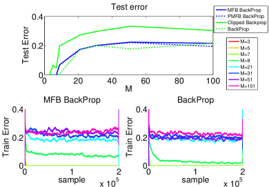
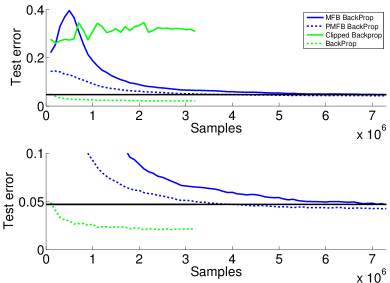
Figure 2: Performance of the MFB-BackProp (and PMFB-BackProp) algorithm on BMNN in comparison with BackProp (and clipped BackProp) on a RMNN with the same architecture. (A) A synthetic teacher student-problem with random inputs. (bottom) MFB-BackProp and BackProp show error during training (top) Mean test error on $10^{4}$ unseen samples, after training has stopped (B) Test error on the MNIST data for a $785\times(301\times 10)\times 10$ 2-layer network. For comparison we give the performance of BackProp on the same network, as well as the performance (black line) of a fully connected ($785\times 300\times 10$) RMNN from the literature (LeCun & Bottou, 1998). The bottom graph “zooms-in” on the asymptotic behavior of the top figure for test error below $0.1$.

To test the MFB-BackProp algorithm, we run numerical experiments on two tasks. The first is a simple teacher-student task with synthetic data. The purpose of this teacher-student scenario is to test the whether the algorithm works properly when (1) the labels are indeed generated by the correct model class (a BMNN), as assumed by our Bayesian framework (2) when the fan-in of the network is small, in contrast to approximation 2. The second task is the standard MNIST handwritten digits recognition task. In this task we examine the performance of our algorithm for relatively large BMNN ($\left|\mathcal{W}\right|=2365860$, while $N=60000$). The purpose of this task was to test whether the algorithm can learn with real-valued inputs and in a more realistic setting, in which the labels $\mathbf{y}$ do not arise from a BMNN teacher, as assumed by the Bayesian approach.

To facilitate comparison, we tested the several algorithms on each task. The output of the network for each algorithms was: (1) MFB-BackProp - the output of a BMNN (Eq. 1) with MAP weights (Eq. 24) estimated by MFB-BackProp (Algorithm 1). (2) PMFB-BackProp - the MAP output (Eq. 25) of a BMNNs estimated by MFB-BackProp (Algorithm 1). (3) BackProp - the output of an RMNN (Eq. 27), trained by standard BackProp (LeCun et al., 2012). We use a RMNN with an identical architecture to the BMNN we train with MFB-BackProp. The RMNN activation function is $s\left(x\right)=1.7159\tanh\left(2x/3\right)$, as recommended by (LeCun et al., 2012) and we select the learning rate $\eta$ by a parameter scan. (4) Clipped-BackProp - the output of the RMNN trained by BackProp, after we clip the weights to be binary (i.e.,$W_{ij,l}^{CBP}=\mathrm{sign}\left(W_{ij,l}^{BP}\right)$).

Note that only MFB-BackProp and Clipped-BackProp yield a MNN with binary weights which can be used for hardware implementations. For all algorithms we used uniform initial conditions, with std=1, as recommended for BackProp (LeCun et al., 2012) - $\sqrt{K_{l}/3}h_{ij,l}^{\left(0\right)}\sim\mathrm{U}\left[-1,1\right]$ for MFB-BackProp, and similarly for $W_{ij,l}^{\left(0\right)}$ in BackProp.

Synthetic Task Implementation.

For all $M\in\left\{3,5,7,9,21,31,51,101\right\}$, we generated synthetic data of $N=2\cdot 10^{5}$ random binary samples $\mathbf{x}^{\left(n\right)}\in\left\{-1,1\right\}^{M}$ and labeled them with $\mathbf{y}^{\left(n\right)}\in\left\{-1,1\right\}$ using a “teacher” - a 2-layer BMNN of size $M\times M\times 1$. We assumed the student knows the architecture of the teacher’s BMNN. However, the teacher’s BMNN’s weights are unknown, and were chosen randomly before each trial of training. The student’s task is to predict the label for each $\mathbf{x}^{\left(n\right)}$, using the outputs of the network for each algorithm. For each algorithm, the classification error is $0$ if the output has the same sign as the label, and $1$ otherwise. During training, the classification error is averaged over the last $5000$ samples. After training has stopped, the test error is given by the mean error of the student on $N=10^{4}$ new random samples of $\mathbf{x}^{\left(n\right)}$. For each $M$, we repeat the training and testing for 10 trials. In Fig. 2A we present the trial with the best test error for each $M$. In the top of Fig. 2A we show the test error of all algorithms we tested. The bottom panels of Fig. 2A show the performance of both the MFB-BackProp and BackProp during training. The learning rate we used for Backprop (selected by a parameter scan for each $M$) were: for $M=3$ $\eta=0.1$, for $M=5,7,9$ $\eta=3\cdot 10^{-2}$, for $M=21,31,51$ $\eta=3\cdot 10^{-3}$ and for $M=101$ $\eta=10^{-3}$.

Synthetic Task Results.

For all algorithms the training error of the network output improves during training (Fig. 2A, bottom). Note that for small networks with $M\leq 7$ the training error reaches zero. As for the test error, MFB-BackProp, PMFB-BackProp and BackProp all have a comparable performance, while Clipped-Backprop performs significantly worse. These results indicate that MFB-BackProp can work rather well, even when the assumption of a “large fan-in” is inaccurate (since $M$ was rather small in some cases).

MNIST Task Implementation.

We tested the algorithms on the standard MNIST handwritten digits database (LeCun & Bottou, 1998). The training set contains $60,000$ images ($28\times 28$ pixels) and the test set has other $10,000$ images. The training set was presented repeatedly, each time with a randomized order of samples. The task was to identify the $\mathrm{label}\in\left\{0,1,\dots 9\right\}$, using a BMNN classier trained by MFB-BackProp (as is standard, we set $y_{k}=2\delta_{k,\mathrm{label}+1}-1$). In all networks we added a constant 1 component to the input, to allow some (small) bias to the neurons in the hidden layer ($V_{0}=785$). Also, we centralized (removed the means) and normalized the input (so $\mathrm{std}=1$), as recommended for BackProp (LeCun et al., 2012). Note that in this task, we know that only a specific set of $10$ pattern is valid (out of possible $2^{10}$). Therefore we need to decide how to classify an image when the network output is “illegal” (e.g., $\left(-1,\dots,-1\right)$). As standard for classification with RMNNs (LeCun & Bottou, 1998), the output neuron which has the highest input indicates the label of the input pattern. We use this classification rule for all algorithms. For BackProp we use $\eta=10^{-3}$, chosen by a parameter scan.

MNIST Task Results.

A fully connected 2-layer ($785\times 300\times 10$) RMNN mentioned in Lecun et al. (1998, Fig. 9), trained using a state-of-the-art (LeCun et al., 2012) Levenberg-Marquardt algorithm, achieved a $4.7\%$ test error. Our goal was to replicate this performance using a BMNN with converging architecture, and so we used a wider BMNN with $785\times(301\times 10)\times 10$ architecture. As can be seen in Fig. 2B, this goal was achieved, since the final test errors were: MFB-BackProp - $4.68\%$, PMFB-BackProp - $4.26\%$. Not surprisingly, the computational capability of a BMNN is somewhat lower than a RMNN of a similar size, since the test error for the RMNN with same architecture were: BackProp - $2.14\%$ and Clipped BackProp - $30.95\%$. An increase in network width (or even better, depth (Siu et al., 1995)) is expected to further improve the performance of the BMNN, but this is left to future work. Note the performance of a SNN in the MNIST task is significantly worse when the weights are constrained to be binary. For example, for a fully connected SNN ($785\times 10$), the test error is $29\%$ for binary weights (using MFB-BackProp, not shown) and $12\%$ (LeCun & Bottou, 1998) for real-valued weights. This demonstrates why our results for the multilayer case are essential for obtaining good performance on realistic tasks.

6 Discussion

Motivated by the recent success of MNNs, and the possibility of implementing them in power-efficient hardware devices requiring limited parameter precision, we developed a Bayesian algorithm for BMNNs. Specifically, we derived the Mean Field-Bayes Backpropagation algorithm - a learning algorithm for BMNNs in which we assumed a converging architecture (i.e., fan-out $1$, except for the input layer).

This online algorithm is essentially an analytic approximation to the intractable Bayes calculation of the posterior distribution of the weights after the arrival of a new data point. Note that this is different from the common MNN training algorithms, such as BackProp, which implement a minimization of some error function. To simplify the intractable Bayes update rule we use two approximations. First, we approximate the posterior using a product of its marginals (a ‘mean field’ approximation). Second, we assume the neuronal layers have a “large” fan-in, so we can use the central limit theorem, as well as first order approximations. After we obtain the approximated updated posterior using the algorithm, it is trivial to find its maximum (due to the posterior’s factorized form).

To the best of our knowledge, this is the first training algorithm for MNNs in general (i.e., not only binary) which is completely Bayesian and scalable (i.e., one which does not use MCMC sampling (MacKay, 1992; Neal, 1995)). Despite its different origin, our algorithm resembles the BackProp algorithm for RMNN - with a specific activation function, learning rate and error function. However, there are a few significant differences. For example, in our algorithm the input to each neuron is scaled adaptively, preserving the amplitude invariance of the BMNN.

As far as we are aware, this is the first scalable algorithm for BMNNs. Interestingly, in the special case of a single layer binary network, our algorithm is almost identical to the online algorithms derived in (Solla & Winther, 1998; Ribeiro & Opper, 2011) (using similar Bayesian formalism and approximations), and the “greedy” version of the belief-propagation based algorithm derived in (Braunstein & Zecchina, 2006). The main difference is the addition of the saturating function $\tanh\left(\cdot\right)$ in our algorithm. Had we used the $\mathrm{sign}\left(\cdot\right)$ function instead, we would have obtained the BPI algorithm (Baldassi et al., 2007).

We test numerically a BMNN trained using our algorithm in a synthetic student-teacher task. The algorithm seems to work well even when the network fan-in is small, in contrast to our assumptions. Next, we test the algorithm on the standard MNIST handwritten digit classification task. We demonstrate that the algorithm can train a 2-layer BMNN (with $\sim 10^{6}$ parameters), and achieve similar performance to 2-layer RMNNs from the literature. In this task, the performance of the 2-layer BMNN is comparable with BackProp tested on the same network (with real weights), and significantly better than the clipped version of BackProp (with binary weights).

The numerical results suggest that 2-layer BMNNs can work just as well as 2-layer RMNN, although they may require a larger width. The weights of the BMNNs we have trained can now be immediately implemented in a hardware chip, such as (Karakiewicz et al., 2012), significantly improving their speed and energy efficiency in comparison to software-based RMNNs. It remains to be seen whether deep BMNNs can compete with RMNNs with (usually, fine tuned) deep architectures, which achieve state-of-the-art performance. To do this, it would be desirable to lift the converging architecture restriction. We hypothesize this constraint can be removed, using the analogy of our algorithm with BackProp. We leave this for future work, as well as quite a few other seemingly straightforward extensions. For example, adapting our formalism to MNNs with discrete weights - i.e., with more than 2 values. In the continuum limit, such a generalization of the algorithm may be used for Bayesian training of RMNNs.

Acknowledgments

The authors are grateful to C. Baldassi, A. Braunstein, and R. Zecchina for helpful discussions and to T. Knafo for reviewing parts of this manuscript. The research was partially funded by the Technion V.P.R. fund and by the Intel Collaborative Research Institute for Computational Intelligence (ICRI-CI).

Supplementary material - derivations

Appendix A The mean-field approximation

In this section we derive of Eqs. 7 and 8. Recall Eq. 5,

$$\hat{P}\left(\mathcal{W}|D_{n}\right)=\prod_{i,j,l}\hat{P}\left(W_{ij,l}|D_{n}\right)\,,$$

where $\hat{P}\left(\mathcal{W}|D_{n}\right)$ is an approximation of $P\left(\mathcal{W}|D_{n}\right)$. In this section we answer the following question - suppose we know $\hat{P}\left(\mathcal{W}|D_{n-1}\right)$. How do we find $\hat{P}\left(\mathcal{W}|D_{n}\right)$? It is a standard approximation to answer this question using a variational approach (see Bishop (2006), and note that Solla & Winther (1998); Ribeiro & Opper (2011) also used the same approach for a SNN with binary weights), through the following two steps:

1. We use the Bayes update (Eq. 3) with $\hat{P}\left(\mathcal{W}|D_{n-1}\right)$ as our prior

   $$\tilde{P}\left(\mathcal{W}|D_{n}\right) \propto P\left(\mathbf{y}^{\left(n\right)}|\mathbf{x}^{\left(n\right)},\mathcal{W}\right)\hat{P}\left(\mathcal{W}|D_{n-1}\right)$$ (32)

   $$= P\left(\mathbf{y}^{\left(n\right)}|\mathbf{x}^{\left(n\right)},\mathcal{W}\right)\prod_{i,j,l}\hat{P}\left(W_{ij,l}|D_{n-1}\right)\,,$$

   where $\tilde{P}\left(\mathcal{W}|D_{n}\right)$ is some “temporary” posterior distribution.

2. We project $\hat{P}\left(\mathcal{W}|D_{n}\right)$ onto $\tilde{P}\left(\mathcal{W}|D_{n}\right)$ by minimizing the reverse Kullback-Leibler divergence (e.g., as in the expectation propagation algorithm Minka (2001); Bishop (2006))

   $$D_{KL}\left(\tilde{P}\left(\mathcal{W}|D_{n}\right)||\hat{P}\left(\mathcal{W}|D_{n}\right)\right)=\sum_{\mathcal{W}}\tilde{P}\left(\mathcal{W}|D_{n}\right)\log\left(\frac{\tilde{P}\left(\mathcal{W}|D_{n}\right)}{\hat{P}\left(\mathcal{W}|D_{n}\right)}\right)$$

   with the normalization constraint $\sum_{W_{ij,l}}\hat{P}\left(W_{ij,l}|D_{n}\right)=1$ $\forall i,j,l$.

The second step can be easily performed using Lagrange multipliers

$$L\left(\hat{P}\left(\mathcal{W}|D_{n}\right)\right)=\sum_{\mathcal{W}^{\prime}}\tilde{P}\left(\mathcal{\mathcal{W}^{\prime}}|D_{n}\right)\log\left(\frac{\tilde{P}\left(\mathcal{W}^{\prime}|D_{n}\right)}{\prod_{k,r,m}\hat{P}\left(W_{kr,m}^{\prime}|D_{n}\right)}\right)+\sum_{k,r,m}\lambda_{kr,m}\left(1-\sum_{W_{kr,m}^{\prime}}\hat{P}\left(W_{kr,m}^{\prime}|D_{n}\right)\right)\,.$$

The minimum is found by differentiating and equating to zero

$$0 = \frac{\partial L\left(\hat{P}\left(\mathcal{W}|D_{n}\right)\right)}{\partial\hat{P}\left(W_{ij,l}|D_{n}\right)}=-\frac{\sum_{\mathbf{\mathcal{W}}^{\prime}:W_{ij,l}^{\prime}=W_{ij,l}}\tilde{P}\left(\mathcal{W}^{\prime}|D_{n}\right)}{\hat{P}\left(W_{ij,l}|D_{n}\right)}-\lambda_{kr,m}\,.$$

Using this equation together with the normalization constraint $\sum_{W_{kr,m}}\hat{P}\left(W_{kr,m}|D_{n}\right)=1$ $\forall k,r,m$ we obtain the result of the minimization through marginalization

$$\hat{P}\left(W_{ij,l}|D_{n}\right) = \sum_{\mathbf{\mathcal{W}}^{\prime}:W_{ij,l}^{\prime}=W_{ij,l}}\tilde{P}\left(\mathcal{W}^{\prime}|D_{n}\right)\,,$$ (33)

which is a known result (Bishop, 2006, p. 468). Finally, we can combine step 1 (Bayes update) with step 2 (projection) to a single step

$$\hat{P}\left(W_{ij,l}|D_{n}\right) = \sum_{\mathbf{\mathcal{W}}^{\prime}:W_{ij,l}^{\prime}=W_{ij,l}}P\left(\mathbf{y}^{\left(n\right)}|\mathbf{x}^{\left(n\right)},\mathbf{\mathcal{W}}^{\prime}\right)\prod_{k,r,m}\hat{P}\left(W_{kr,m}^{\prime}|D_{n-1}\right)\,.$$

This step is exactly Eqs. 7 and 8 combined.

Appendix B Forward propagation of probabilities

In this section we simplify the summations in Eqs. (11-15), by assuming that the fan-in of all of the connections is “large”, i.e., $\forall m:K_{m}\rightarrow\infty$. Recall (from Eq. 9) that $W_{ij,l}$ is a specific weight which is fixed (so $i,j$ and $l$ are “special” indexes), while all the other weights $W_{kr,m}$ (for which $k\neq i$ or $r\neq j$ or $m\neq l$) are independent binary random variables with $P\left(W_{kr,m}=1\right)=1-P\left(W_{kr,m}=-1\right),\,\forall k,r,m$.

B.1 Some more preliminaries

In addition to the notations defined in the the paper, we introduce the following notation:

1. We use here a $x^{\pm}$ as a shorthand for $x=\pm 1$ (so for example, we write $P\left(y=1|x=-1\right)$ as $P\left(y^{+}|x^{-}\right)$.

2. $\mathrm{Var}\left[x\right]=\left\langle X^{2}\right\rangle-\left\langle X\right\rangle^{2}$

Also, recall that for a binary variable $X$, we have

$$P\left(X=1\right) = P\left(X^{+}\right)=1-P\left(X^{-}\right)$$

$$\left\langle X\right\rangle = P\left(X^{+}\right)-P\left(X^{-}\right)=2P\left(X^{+}\right)-1\,.$$ (34)

$$\left\langle X^{2}\right\rangle = 1$$

$$\mathrm{Var}\left[X\right] = 1-\left\langle X\right\rangle^{2}$$ (35)

B.2 First layer

In this subsection we calculate $P\left(\mathbf{v}_{1}\right)$, defined in Eq. 12, assuming $l\neq 1$. In this layer the input is a fixed real vector $\mathbf{v}_{0}=\mathbf{x}\in\mathbb{R}^{V_{0}}$ (this is different from the next layers, where the input will be a binary random vector).

Using Eqs. 12 and 11, the fact that the weights are binary and the central limit theorem we obtain

$$P\left(\mathbf{v}_{1}\right) = P\left(\mathbf{v}_{1}|\mathbf{v}_{0}=\mathbf{x}\right)$$ (36)

$$= \sum_{\mathbf{W}_{1}^{\prime}}\prod_{k}\left[\theta\left(v_{k,1}\frac{1}{\sqrt{K_{1}}}\sum_{r\in K\left(k,1\right)}x_{r}W_{kr,1}^{\prime}\right)\prod_{r\in K\left(k,1\right)}P\left(W_{kr,1}^{\prime}\right)\right]$$ (37)

$$\approx \prod_{k}\left[\int_{-\infty}^{\infty}\theta\left(v_{k,1}u_{k,1}\right)\mathcal{N}\left(u_{k,1}|\mu_{k,1},\sigma_{k,1}^{2}\right)du_{k,1}\right]\,,$$ (38)

$$= \prod_{k}\Phi\left(\frac{v_{k,1}\mu_{k,1}}{\sigma_{k,1}}\right)\,,$$ (39)

where in the approximated equality we changed the summation on $\mathbf{W}_{1}^{\prime}$ to a Gaussian integration on

$$u_{k,1}=\frac{1}{\sqrt{K_{1}}}\sum_{r\in K\left(k,1\right)}x_{r}W_{kr,1}^{\prime}\sim\mathcal{N}\left(\mu_{k,1},\sigma_{k,1}^{2}\right)\,,$$

for which

$$\mu_{k,1} = \left\langle u_{k,m}\right\rangle$$ (40)

$$= \left\langle\frac{1}{\sqrt{K_{1}}}\sum_{r\in K\left(k,1\right)}x_{r}W_{kr,1}^{\prime}\right\rangle$$

$$= \frac{1}{\sqrt{K_{1}}}\sum_{r\in K\left(k,1\right)}\left\langle W_{kr,1}\right\rangle x_{k}\,,$$ (41)

$$\sigma_{k,1}^{2} = \mathrm{Var}\left[u_{k,m}\right]$$ (42)

$$= \mathrm{Var}\left[\frac{1}{\sqrt{K_{1}}}\sum_{r\in K\left(k,1\right)}x_{r}W_{kr,1}^{\prime}\right]$$

$$= \frac{1}{K_{1}}\sum_{r\in K\left(k,1\right)}x_{r}^{2}\mathrm{Var}\left[W_{kr,1}^{\prime}\right]$$ (43)

$$= \frac{1}{K_{1}}\sum_{r\in K\left(k,1\right)}x_{r}^{2}\left(1-\left\langle W_{kr,1}\right\rangle^{2}\right),$$ (44)

where we used Eq. 35 (recall also that $W^{\pm}$ means $W=\pm 1$). Note that from Eq. 39 we obtained that the outputs of the first layer are independent

$$P\left(\mathbf{v}_{1}\right)=\prod_{k}P\left(v_{k,1}\right)=\prod_{k}\Phi\left(v_{k,1}\mu_{k,1}/\sigma_{k,1}\right)\,.$$ (45)

Also note, that if $\left|\mu_{k,1}\right|\gg\sigma_{k,1}$, our CLT-based approximation in Eq. 38 breaks down. Despite this, in this limit, $P\left(v_{k,1}\right)\approx\theta\left(v_{k,1}\mu_{k,1}\right)$ with or without the approximation. However, is is important to note that the asymptotic form at which we approach this limit is different without the CLT-based approximation.

B.3 Layers $m=2,3,\dots,l$

In this subsection we calculate $P\left(\mathbf{v}_{m}\right)$ $\forall m\in\left\{2,..,l-1\right\}$, as defined in Eq. 13. In this layer the input is a random binary vector $\mathbf{v}_{m-1}\in\left\{-1,1\right\}^{V_{m-1}}$. From Eq. 45 we know that the inputs are independent for $m=2$ (i.e., $P\left(\mathbf{v}_{1}\right)=\prod_{k}P\left(v_{k,1}\right)$). We assume this is true $\forall m$, and this proved by induction ($i.e.$, assuming $P\left(\mathbf{v}_{m}\right)=\prod_{k}P\left(v_{k,m}\right)$ will yield $P\left(\mathbf{v}_{m+1}\right)=\prod_{k}P\left(v_{k,m+1}\right)$).

Using Eqs. 11 and 13, we can perform very similar calculation for as we did for the first layer

$$P\left(\mathbf{v}_{m}\right) = \sum_{\mathbf{v}_{m-1}}\sum_{\mathbf{W}_{m}^{\prime}}\prod_{k}\left[\theta\left(v_{k,m}\frac{1}{\sqrt{K_{m}}}\sum_{r\in K\left(k,m\right)}v_{m-1}W_{kr,m}^{\prime}\right)\prod_{r\in K\left(k,m\right)}P\left(W_{kr,m}^{\prime}\right)P\left(v_{r,m-1}\right)\right]$$

$$\approx \prod_{k}\left[\int_{-\infty}^{\infty}\theta\left(v_{k,m}u_{k,m}\right)\mathcal{N}\left(u_{k,m}|\mu_{k,m},\sigma_{k,m}^{2}\right)du_{k,m}\right]\,,$$

$$= \prod_{k}\Phi\left(\frac{v_{k,m}\mu_{k,m}}{\sigma_{k,m}}\right)\,,$$

where we similarly approximated

$$u_{k,m}=\frac{1}{\sqrt{K_{m}}}\sum_{r\in K\left(k,m\right)}v_{r,m-1}W_{kr,m}^{\prime}\sim\mathcal{N}\left(\mu_{k,m},\sigma_{k,m}^{2}\right)\,,$$

for which

$$\mu_{k,m} = \left\langle\frac{1}{\sqrt{K_{m}}}\sum_{r\in K\left(k,m\right)}v_{r,m-1}W_{kr,m}^{\prime}\right\rangle$$ (47)

$$= \frac{1}{\sqrt{K_{m}}}\sum_{r\in K\left(k,m\right)}\left\langle W_{kr,m}\right\rangle\left\langle v_{r,m-1}\right\rangle\,,$$

$$\sigma_{k,m}^{2} = \mathrm{Var}\left[\frac{1}{\sqrt{K_{m}}}\sum_{r\in K\left(k,m\right)}v_{r,m-1}W_{kr,m}^{\prime}\right]$$ (48)

$$= \frac{1}{K_{m}}\sum_{r\in K\left(k,m\right)}\mathrm{Var}\left[v_{r,m-1}W_{kr,m}^{\prime}\right]$$

$$= \frac{1}{K_{m}}\sum_{r\in K\left(k,m\right)}\left(1-\left\langle v_{r,m-1}\right\rangle^{2}\left\langle W_{kr,m}\right\rangle^{2}\right)\,,$$

with

$$\left\langle v_{r,m-1}\right\rangle=2P\left(v_{k,m-1}^{+}\right)-1=2\Phi\left(\mu_{k,m}/\sigma_{k,m}\right)-1\,.$$ (49)

Again, if $\left|\mu_{k,m}\right|\gg\sigma_{k,m}$, our CLT-based approximation in Eq. B.3 breaks down, but $P\left(v_{k,m}\right)\approx\theta\left(v_{k,m}\mu_{k,m}\right)$ holds even then. Again, the asymptotic form at which we approach this limit is different without the CLT-based approximation. Also, we got that the outputs are independent $P\left(\mathbf{v}_{m}\right)=\prod_{k}P\left(v_{k,m}\right)$, so we can similarly calculate $P\left(\mathbf{v}_{m+1}\right)$ for $\forall m>1$.

B.4 Layer $l$

In this subsection we calculate $P\left(\mathbf{v}_{l}|W_{ij,l}\right)$, as defined in Eq. 14. We will have to consider two different cases here - when $l=1$ and when $l\neq 1$, since we have different type of inputs to the layer in each case. Note that since $W_{ij,l}$ is a “special” fixed weight (see Eq. 9), we will have to redefine $\mathbf{u}_{l}$ (originally defined in Eq. 16) as if $W_{ij,l}$ “disconnected”.

B.4.1 Case when $l\neq 1$

First, we re-define $\mathbf{u}_{l}$ in this layer, so that

$$u_{k,l}=\begin{cases}\frac{1}{\sqrt{K_{l}}}\sum_{r\in K\left(k,l\right)}v_{r,l-1}W_{kr,l}^{\prime}\,\,\,\sim\mathcal{N}\left(\mu_{k,l},\sigma_{k,l}^{2}\right)&,\,\mathrm{if}\,\,k\neq i\\ \frac{1}{\sqrt{K_{l}}}\sum_{r\in K\left(k,l\right)\backslash j}v_{r,l-1}W_{kr,l}^{\prime}\,\sim\mathcal{N}\left(\mu_{i\left(j\right),l},\sigma_{i\left(j\right),l}^{2}\right)&,\,\mathrm{if}\,\,k=i\end{cases}\,.$$

Now, $\mu_{k,l}$ and $\sigma_{k,l}$ are defined as in Eqs. 47-48, while

$$\mu_{i\left(j\right),l} = \left\langle u_{i,l}\right\rangle$$ (50)

$$= \frac{1}{\sqrt{K_{l}}}\sum_{r\in K\left(i,l\right)\backslash j}\left\langle W_{ir,l}\right\rangle\left\langle v_{r,l-1}\right\rangle\,,$$

$$\sigma_{i\left(j\right),l}^{2} = \mathrm{Var}\left[u_{i,l}\right]$$ (51)

$$= \frac{1}{K_{l}}\sum_{r\in K\left(i,l\right)\backslash j}\left(1-\left\langle v_{r,l-1}\right\rangle^{2}\left\langle W_{ir,l}\right\rangle^{2}\right)\,,$$

Next, using similar methods (as we did before) on Eq. 14 (with $P\left(\mathbf{v}_{l}|\mathbf{v}_{l-1},W_{ij,l}\right)$ defined immediately after Eq. 11), we have

$$P\left(\mathbf{v}_{l}|W_{ij,l}\right)$$ (52)

$$= \sum_{\mathbf{v}_{l-1}}\sum_{\mathbf{W}_{l}^{\prime}:W_{ij,l}^{\prime}=W_{ij,l}}\left[\left(P\left(W_{ij,l}\right)\right)^{-1}\prod_{k}\theta\left(v_{k,l}\frac{1}{\sqrt{K_{l}}}\sum_{r\in K\left(k,l\right)}v_{r,l-1}W_{kr,l}^{\prime}\right)\prod_{r\in K\left(k,l\right)}P\left(W_{kr,l}^{\prime}\right)P\left(v_{r,l-1}\right)\right]P\left(v_{j,l-1}\right)$$

$$\approx \left[\prod_{k\neq i}\Phi\left(\frac{v_{k,l}\mu_{k,l}}{\sigma_{k,l}}\right)\right]\sum_{v_{j,l-1}}\Phi\left(\frac{v_{i,l}}{\sigma_{i\left(j\right),l}}\left(\mu_{i\left(j\right),l}+\frac{1}{\sqrt{K_{l}}}W_{ij,l}v_{j,l-1}\right)\right)P\left(v_{j,l-1}\right)\,$$

$$= \left[\prod_{k\neq i}P\left(v_{k,l}\right)\right]P\left(v_{i,l}|W_{ij,l}\right)\,.$$ (53)

If $\sigma_{i\left(j\right),l}\gg 1/\sqrt{K_{l}}$ (which can be reasonable if $K_{l}$ is large) then we can perform a first order Taylor expansion of the last line and obtain

$$P\left(v_{i,l}|W_{ij,l}\right) = \sum_{v_{j,l-1}}\Phi\left(\frac{v_{i,l}}{\sigma_{i\left(j\right),l}}\left(\mu_{i\left(j\right),l}+\frac{1}{\sqrt{K_{l}}}W_{ij,l}v_{j,l-1}\right)\right)P\left(v_{j,l-1}\right)$$ (54)

$$\approx \sum_{v_{j,l-1}}\left[\Phi\left(\frac{v_{i,l}\mu_{i\left(j\right),l}}{\sigma_{i\left(j\right),l}}\right)+\frac{1}{\sqrt{K_{l}}}\mathcal{N}\left(0|\mu_{i\left(j\right),l},\sigma_{i\left(j\right),l}^{2}\right)W_{ij,l}v_{i,l}v_{j,l-1}\right]P\left(v_{j,l-1}\right)$$

$$= \Phi\left(\frac{v_{i,l}\mu_{i\left(j\right),l}}{\sigma_{i\left(j\right),l}}\right)+\frac{1}{\sqrt{K_{l}}}\mathcal{N}\left(0|\mu_{i\left(j\right),l},\sigma_{i\left(j\right),l}^{2}\right)W_{ij,l}v_{i,l}\left\langle v_{j,l-1}\right\rangle\,.$$ (55)

However, if $\left|\mu_{i\left(j\right),l}\right|\ll 1/\sqrt{K_{l}}$ and $\sigma_{i\left(j\right),l}\ll 1/\sqrt{K_{l}}$ we can obtain instead (even though the CLT is not valid)

$$P\left(v_{i,l}|W_{ij,l}\right) = \sum_{v_{j,l-1}}\theta\left(v_{i,l}W_{ij,l}v_{j,l-1}\right)P\left(v_{j,l-1}\right)$$ (56)

$$= \frac{1}{2}\left(1+W_{ij,l}v_{i,l}\left\langle v_{j,l-1}\right\rangle\right)\,.$$ (57)

Note that this separation of the last two limit cases is particularly important, since if we use Eq. 55 in the second case, the equation will diverge. Both limit cases can be heuristically combined into one equation

$$P\left(v_{i,l}|W_{ij,l}\right) \approx \Phi\left(\frac{v_{i,l}\mu_{i\left(j\right),l}}{\sigma_{i\left(j\right),l}}\right)+\frac{1}{2}\tanh\left[\frac{2}{\sqrt{K_{l}}}\mathcal{N}\left(0|\mu_{i\left(j\right),l},\sigma_{i\left(j\right),l}^{2}\right)\right]W_{ij,l}v_{i,l}\left\langle v_{j,l-1}\right\rangle\,,$$ (58)

since

$$\tanh\left(x\right)\approx\begin{cases}x&,\,\,\mathrm{if}\,\left|x\right|\ll 1\\ \mathrm{sign\left(x\right)}&,\,\,\mathrm{if}\,\left|x\right|\gg 1\end{cases}\,.$$

Importantly, since the two limit cases were “glued” heuristically, Eq. 58 does not give the asymptotic form at which we approach the limit $\left|\mu_{i\left(j\right),l}\right|\ll 1/\sqrt{K_{l}}$ and $\sigma_{i\left(j\right),l}\ll 1/\sqrt{K_{l}}$. Also, if $\left|\mu_{i\left(j\right),l}\right|\gg\sigma_{i\left(j\right),l}$ and also $\left|\mu_{i\left(j\right),l}\right|>1/\sqrt{K_{l}}$ the assumptions behind Eq. 58 break down, but the result $P\left(v_{i,l}|W_{ij,l}\right)\approx\theta\left(v_{i,l}\mu_{i\left(j\right),l}\right)$ remains. Again, the asymptotic form at which we approach this limit is different without the CLT-based approximation.

B.4.2 Case when $l=1$

In this case, we re-define $\mathbf{u}_{l}$ in this layer, so that

$$u_{k,l}=\begin{cases}\frac{1}{\sqrt{K_{l}}}\sum_{r\in K\left(k,l\right)}x_{r,}W_{kr,l}^{\prime}\,\,\,\sim\mathcal{N}\left(\mu_{k,l},\sigma_{k,l}^{2}\right)&,\,\mathrm{if}\,\,k\neq i\\ \frac{1}{\sqrt{K_{l}}}\sum_{r\in K\left(k,l\right)\backslash j}x_{r}W_{kr,l}^{\prime}\,\sim\mathcal{N}\left(\mu_{i\left(j\right),l},\sigma_{i\left(j\right),l}^{2}\right)&,\,\mathrm{if}\,\,k=i\end{cases}$$

with $\mu_{k,l}$ and $\sigma_{k,l}$ are defined as in Eqs. 41-44, while

$$\mu_{i\left(j\right),l} = \frac{1}{\sqrt{K_{l}}}\sum_{r\in K\left(i,l\right)\backslash j}\left\langle W_{ir,l}\right\rangle x_{r}\,,$$ (59)

$$\sigma_{i\left(j\right),l}^{2} = \frac{1}{K_{l}}\sum_{r\in K\left(i,l\right)\backslash j}x_{r}^{2}\left(1-\left\langle W_{ir,l}\right\rangle^{2}\right)\,.$$ (60)

Thus, we obtain

$$P\left(\mathbf{v}_{l}|W_{ij,l}\right)$$

$$= \sum_{\mathbf{W}_{l}^{\prime}:W_{ij,l}^{\prime}=W_{ij,l}}\left[\left(P\left(W_{ij,l}\right)\right)^{-1}\prod_{k}\theta\left(v_{k,l}\frac{1}{\sqrt{K_{l}}}\sum_{r\in K\left(k,l\right)}x_{r,l-1}W_{kr,l}^{\prime}\right)\prod_{r\in K\left(k,l\right)}P\left(W_{kr,l}^{\prime}\right)\right]$$

$$\approx \left[\prod_{k\neq i}\Phi\left(\frac{v_{k,l}\mu_{k,l}}{\sigma_{k,l}}\right)\right]\Phi\left(\frac{v_{i,l}}{\sigma_{i\left(j\right),l}}\left(\mu_{i\left(j\right),l}+\frac{1}{\sqrt{K_{l}}}W_{ij,l}x_{j}\right)\right)$$

$$= \left[\prod_{k\neq i}P\left(v_{k,l}\right)\right]P\left(v_{i,l}|W_{ij,l}\right)\,.$$

If $\left|\mu_{i\left(j\right),l}\right|\gg x_{j}/\sqrt{K_{l}}$ or $\sigma_{i\left(j\right),l}\gg x_{j}/\sqrt{K_{l}}$ then we can perform a first order Taylor expansion of the last line and obtain

$$P\left(v_{i,l}|W_{ij,l}\right)=\Phi\left(\frac{v_{i,l}\mu_{i\left(j\right),l}}{\sigma_{i\left(j\right),l}}\right)+\frac{1}{\sqrt{K_{l}}}\mathcal{N}\left(0|\mu_{i\left(j\right),l},\sigma_{i\left(j\right),l}^{2}\right)W_{ij,l}v_{i,l}x_{j}\,.$$ (61)

and if $\left|\mu_{i\left(j\right),l}\right|\ll x_{j}/\sqrt{K_{l}}$ and $\sigma_{i\left(j\right),l}\ll x_{j}/\sqrt{K_{l}}$, we obtain instead

$$P\left(v_{i,l}|W_{ij,l}\right)=\frac{1}{2}\left(1+v_{i,l}W_{ij,l}\mathrm{sign}\left(x_{j}\right)\right)$$

Both limit cases can be again combined into a single equation

$$P\left(v_{i,l}|W_{ij,l}\right) \approx \Phi\left(\frac{v_{i,l}\mu_{i\left(j\right),l}}{\sigma_{i\left(j\right),l}}\right)+\frac{1}{2}\tanh\left[\frac{2}{\sqrt{K_{l}}}\mathcal{N}\left(0|\mu_{i\left(j\right),l},\sigma_{i\left(j\right),l}^{2}\right)x_{j}\right]W_{ij,l}v_{i,l}\,.$$ (62)

Again, if $\left|\mu_{i\left(j\right),l}\right|\gg\sigma_{i\left(j\right),l}$, the assumptions behind Eq. 58 breaks down, but in that limit we still have $P\left(v_{i,l}|W_{ij,l}\right)\approx\theta\left(v_{i,l}\left(\mu_{i\left(j\right),l}+W_{ij,l}x_{j}/\sqrt{K_{l}}\right)\right)$. Again, the asymptotic form at which we approach this limit is different without the CLT-based approximation.

B.5 Layers $m=l+1,l+2\dots,L$

In this subsection we calculate $P\left(\mathbf{v}_{m}|W_{ij,l}\right),$ $\forall m\geq l$, as defined in Eq. 15. We denote $c\left(i,l,l^{\prime}\right)$ (’child’) to be the index of the neuron in the $l^{\prime}$ layer which is receiving input (through other neurons) from the $i$-th neuron in the $l$ layer, and $i_{m}=c\left(i,l,m\right)$ and $j_{m}=c\left(i,l,m-1\right)$. Using similar methods (as before) on Eqs. 11 and 15, we obtain

$$P\left(\mathbf{v}_{m}|W_{ij,l}\right)=\left[\prod_{k\neq i_{m}}\Phi\left(\frac{v_{k,m}\mu_{k,m}}{\sigma_{k,m}}\right)\right]P\left(v_{i_{m},m}|W_{ij,l}\right)$$

with

$$P\left(v_{i_{m},m}|W_{ij,l}\right)$$ (63)

$$= \sum_{\mathbf{v}_{m-1},\mathbf{W}_{m}^{\prime}}\theta\left(v_{i_{m},m}\frac{1}{\sqrt{K_{m}}}\sum_{r\in K\left(i_{m},m\right)}v_{r,m-1}W_{i_{m}r,m}^{\prime}\right)\prod_{r\in K\left(i_{m},m\right)}P\left(W_{i_{m}r,m}^{\prime}\right)\prod_{r\in K\left(i_{m},m\right)\backslash j_{m}}P\left(v_{r,m-1}\right)P\left(v_{j_{m},m-1}|W_{ij,l}\right)$$

$$\approx \sum_{v_{j_{m},m-1},W_{i_{m}j_{m},m}^{\prime}}\Phi\left(\frac{v_{i_{m},m}}{\sigma_{i_{m}\left(j_{m}\right),m}}\left(\mu_{i_{m}\left(j_{m}\right),m}+\frac{1}{\sqrt{K_{m}}}W_{i_{m}j_{m},m}v_{j_{m},m-1}\right)\right)P\left(W_{i_{m}j_{m},m}^{\prime}\right)P\left(v_{j_{m},m-1}|W_{ij,l}\right)\,,$$

$$\approx \Phi\left(\frac{v_{i_{m},m}\mu_{i_{m}\left(j_{m}\right),m}}{\sigma_{i_{m}\left(j_{m}\right),m}}\right)+\frac{1}{2}\tanh\left[\frac{2}{\sqrt{K_{m}}}\mathcal{N}\left(0|\mu_{i_{m}\left(j_{m}\right),m},\sigma_{i_{m}\left(j_{m}\right),m}^{2}\right)\right]\left\langle W_{i_{m}j_{m},m}\right\rangle v_{i_{m},m}\left\langle v_{j_{m},m-1}|W_{ij,l}\right\rangle$$ (64)

where $\mu_{k,m}$ and $\sigma_{k,m}$ are defined as in Eqs. 47-48, $\mu_{i_{m}\left(j_{m}\right),m}$ and $\sigma_{i_{m}\left(j_{m}\right),m}$ are defined as in Eqs. 50-51 and again we divided into two limits, as in Eq. 58. Also, if $\left|\mu_{i_{m}\left(j_{m}\right),m}\right|\gg\sigma_{i_{m}\left(j_{m}\right),m}$ and $\left|\mu_{i_{m}\left(j_{m}\right),m}\right|>1/\sqrt{K_{m}}$ our assumptions break down but we still have $P\left(v_{i_{m},m}|W_{ij,l}\right)\approx\theta\left(v_{i_{m},m}\mu_{i_{m}\left(j_{m}\right),m}\right)$. Again, the asymptotic form at which we approach this limit is different without the CLT-based approximation.

Appendix C The log-likelihood ratio

Using the results from the previous section, we can now calculate $P\left(\mathbf{y}|W_{ij,l}\right)=P\left(\mathbf{v}_{L}=\mathbf{y}|W_{ij,l}\right)$ for every $W_{ij,l}$ . We instead calculate the following, equivalently useful, log-likelihood ratio

$$R_{ij,l}=\ln\frac{P\left(\mathbf{y}|W_{ij,l}^{+}\right)}{P\left(\mathbf{y}|W_{ij,l}^{-}\right)}\,.$$ (65)

This quantity is useful, since, from Eq. 7, it uniquely determines the Bayes updates of the posterior as

$$\ln\frac{P\left(W_{ij,l}^{+}|D_{n}\right)}{P\left(W_{ij,l}^{-}|D_{n}\right)}=\ln\frac{P\left(W_{ij,l}^{+}|D_{n-1}\right)}{P\left(W_{ij,l}^{-}|D_{n-1}\right)}+R_{ij,l}^{\left(n\right)}\,.$$

Next, we assume that $R_{ij,l}\ll 1$ and discuss the complementary case towards the end of this section. If $l=L=1$, then, using Eq. 62, we find

$$R_{ij,l} = \ln\frac{\Phi\left(\frac{y_{i}\mu_{i\left(j\right),L}}{\sigma_{i\left(j\right),L}}\right)+\frac{1}{2}\tanh\left[\frac{2}{\sqrt{K_{L}}}\mathcal{N}\left(0|\mu_{i\left(j\right),L},\sigma_{i\left(j\right),L}^{2}\right)x_{j}y_{i}\right]}{\Phi\left(\frac{y_{i}\mu_{i\left(j\right),L}}{\sigma_{i\left(j\right),L}}\right)-\frac{1}{2}\tanh\left[\frac{2}{\sqrt{K_{L}}}\mathcal{N}\left(0|\mu_{i\left(j\right),L},\sigma_{i\left(j\right),L}^{2}\right)x_{j}y_{i}\right]}$$ (66)

$$\approx \ln\frac{1+\frac{1}{2}\tanh\left[\frac{2\mathcal{N}\left(0|\mu_{i\left(j\right),L},\sigma_{i\left(j\right),L}^{2}\right)}{\sqrt{K_{L}}\Phi\left(y_{i}\mu_{i\left(j\right),L}/\sigma_{i\left(j\right),L}\right)}x_{j}y_{i}\right]}{1-\frac{1}{2}\tanh\left[\frac{2\mathcal{N}\left(0|\mu_{i\left(j\right),L},\sigma_{i\left(j\right),L}^{2}\right)}{\sqrt{K_{L}}\Phi\left(y_{i}\mu_{i\left(j\right),L}/\sigma_{i\left(j\right),L}\right)}x_{j}y_{i}\right]}$$

$$\approx \tanh\left[\frac{2}{\sqrt{K_{L}}}\frac{\mathcal{N}\left(0|\mu_{i\left(j\right),L},\sigma_{i\left(j\right),L}^{2}\right)}{\Phi\left(y_{i}\mu_{i\left(j\right),L}/\sigma_{i\left(j\right),L}\right)}x_{j}y_{i}\right]\,.$$ (67)

where we used a first order Taylor expansion, assuming $R_{ij,l}\ll 1$.

If $l=L>1$, then, using Eq. 58, we find

$$R_{ij,l} = \ln\frac{\Phi\left(\frac{y_{i}\mu_{i\left(j\right),L}}{\sigma_{i\left(j\right),L}}\right)+\frac{1}{2}\tanh\left[\frac{2}{\sqrt{K_{L}}}\mathcal{N}\left(0|\mu_{i\left(j\right),L},\sigma_{i\left(j\right),L}^{2}\right)y_{i}\right]\left\langle v_{j,L-1}\right\rangle}{\Phi\left(\frac{y_{i}\mu_{i\left(j\right),L}}{\sigma_{i\left(j\right),L}}\right)-\frac{1}{2}\tanh\left[\frac{2}{\sqrt{K_{L}}}\mathcal{N}\left(0|\mu_{i\left(j\right),L},\sigma_{i\left(j\right),L}^{2}\right)y_{i}\right]\left\langle v_{j,L-1}\right\rangle}$$ (68)

$$\approx \tanh\left[\frac{2}{\sqrt{K_{L}}}\frac{\mathcal{N}\left(0|\mu_{i\left(j\right),L},\sigma_{i\left(j\right),L}^{2}\right)}{\Phi\left(y_{i}\mu_{i\left(j\right),L}/\sigma_{i\left(j\right),L}\right)}y_{i}\right]\left\langle v_{j,L-1}\right\rangle\,,$$

where we used a first order Taylor expansion, assuming $R_{ij,l}\ll 1$.

Next, for $l<L$, we denote $c\left(i,l,l^{\prime}\right)$ to be the index of the neuron in the $l^{\prime}$ layer which is receiving input (through other neurons) from the $i$-th neuron in the $l$ layer, and $i_{m}=c\left(i,l,m\right)$ and $j_{m}=c\left(i,l,m-1\right)$. We obtain

$$R_{ij,l} \approx \ln\frac{\Phi\left(\frac{y_{i_{L}}\mu_{i_{L}\left(j_{L}\right),L}}{\sigma_{i_{L}\left(j_{L}\right),L}}\right)+\frac{1}{2}\tanh\left[\frac{2}{\sqrt{K_{L}}}\mathcal{N}\left(0|\mu_{i_{L}\left(j_{L}\right),L},\sigma_{i_{L}\left(j_{L}\right),L}^{2}\right)y_{i_{L}}\right]\left\langle W_{i_{L}j_{L},L}\right\rangle\left\langle v_{j_{L},L-1}|W_{ij,l}^{+}\right\rangle}{\Phi\left(\frac{y_{i_{L}}\mu_{i_{L}\left(j_{L}\right),L}}{\sigma_{i_{L}\left(j_{L}\right),L}}\right)+\frac{1}{2}\tanh\left[\frac{2}{\sqrt{K_{L}}}\mathcal{N}\left(0|\mu_{i_{L}\left(j_{L}\right),L},\sigma_{i_{L}\left(j_{L}\right),L}^{2}\right)y_{i_{L}}\right]\left\langle W_{i_{L}j_{L},L}\right\rangle\left\langle v_{j_{L},L-1}|W_{ij,l}^{-}\right\rangle}$$ (69)

$$\approx \tanh\left[\frac{2}{\sqrt{K_{L}}}\frac{\mathcal{N}\left(0|\mu_{i_{L}\left(j_{L}\right),L},\sigma_{i_{L}\left(j_{L}\right),L}^{2}\right)}{\Phi\left(y_{i_{L}}\mu_{i_{L}\left(j_{L}\right),L}/\sigma_{i_{L}\left(j_{L}\right),L}\right)}y_{i_{L}}\right]\left\langle W_{i_{L}j_{L},L}\right\rangle\left(\left\langle v_{j_{L},L-1}|W_{ij,l}^{+}\right\rangle-\left\langle v_{j_{L},L-1}|W_{ij,l}^{-}\right\rangle\right)\,,$$

where we used a first order Taylor expansion, assuming $R_{ij,l}\ll 1$ . We can now continue and apply Eq. 64 for $m=L-1,L-2,\dots,l+1$, obtaining the recursive relation

$$\frac{\left\langle v_{i{}_{m},m}|W_{ij,l}^{+}\right\rangle-\left\langle v_{i_{m},m}|W_{ij,l}^{-}\right\rangle}{\left\langle v_{i{}_{m-1},m-1}|W_{ij,l}^{+}\right\rangle-\left\langle v_{i_{m-1},m-1}|W_{ij,l}^{-}\right\rangle}\approx\tanh\left[\frac{2}{\sqrt{K_{m}}}\mathcal{N}\left(0|\mu_{i_{m}\left(j_{m}\right),m},\sigma_{i_{m}\left(j_{m}\right),m}^{2}\right)\right]\left\langle W_{i_{m}j_{m},m}\right\rangle$$ (70)

We can now continue to apply Eq. 64, until we reach layer $l$, for which we need to use Eq. 58 to obtain

$$\left\langle v_{i,l}|W_{ij,l}^{+}\right\rangle-\left\langle v_{i,l}|W_{ij,l}^{-}\right\rangle\approx\tanh\left[\frac{2}{\sqrt{K_{l}}}\mathcal{N}\left(0|\mu_{i\left(j\right),l},\sigma_{i\left(j\right),l}^{2}\right)\right]\left\langle v_{j,l-1}\right\rangle$$ (71)

or, if $l=1$

$$\left\langle v_{i,l}|W_{ij,l}^{+}\right\rangle-\left\langle v_{i,l}|W_{ij,l}^{-}\right\rangle\approx\tanh\left[\frac{2}{\sqrt{K_{l}}}\mathcal{N}\left(0|\mu_{i\left(j\right),l},\sigma_{i\left(j\right),l}^{2}\right)x_{j}\right]\,.$$ (72)

Lastly, we note so far we assumed $R_{ij,l}\ll 1$. This is not always the case. For example, if $P\left(\mathbf{y}|W_{ij,l}^{-}\right)\rightarrow 0$ and/or $P\left(\mathbf{y}|W_{ij,l}^{+}\right)\rightarrow 0$, $R_{ij,l}$ may diverge. In this case the CLT theorem we used becomes invalid, so we cannot use the expressions we previously found in section B to obtain the correct asymptotic form in this limit - only the sign of $R_{ij,l}$. From the conditions for the validity of the CLT we can see qualitatively that this can occur if a highly “unexpected” sample $\left\{\mathbf{x}^{\left(n\right)},\mathbf{y}^{\left(n\right)}\right\}$ arrive, when “certainty” of the posteriors increase - i.e. they converge either to zero or one. Unfortunately, as we stated, the value of the log-likelihood (Eq. 65) can diverge, so the effects on the learning process can be quite destructive. As an ad-hoc solution, in order to ward against the destructive effect of such divergent errors, we just use the above expression even $R_{ij,l}\ll 1$ is no longer true. In this case we will have some error in our estimate of $R_{ij,l}$, but at least it will have the right sign and will be finite in each time-step. Of course, even “small” errors can sometimes accumulate significantly over long time, and we have no mathematical guarantee this will not happen.

Appendix D Summary

Next, we summarize our main results. This also appears in the paper, but here we also give reference to the specific equations in the derivations.

In the section B we defined (combining the definitions in Eqs. 41, 44, 47 and 48)

$$\mu_{k,m} = \frac{1}{\sqrt{K_{m}}}\sum_{r\in K\left(k,m\right)}\left\langle W_{kr,m}\right\rangle\left\langle v_{r,m-1}\right\rangle$$

$$\sigma_{k,m}^{2} = \frac{1}{K_{m}}\sum_{r\in K\left(k,m\right)}\left(\delta_{1m}\left(\left\langle v_{r,m-1}\right\rangle^{2}-1\right)+1-\left\langle v_{r,m-1}\right\rangle^{2}\left\langle W_{kr,m}\right\rangle^{2}\right)$$

and (combining the definitions in Eqs. 50-51 with the two previous equations)

$$\mu_{i\left(j\right),l} = \mu_{i,l}-\frac{1}{\sqrt{K_{l}}}\left\langle W_{ij,l}\right\rangle\left\langle v_{j,l-1}\right\rangle$$

$$\sigma_{i\left(j\right),l}^{2} = \sigma_{i,l}^{2}-\frac{1}{K_{l}}\left(\delta_{1l}\left(\left\langle v_{j,l-1}\right\rangle^{2}-1\right)+1-\left\langle v_{j,l-1}\right\rangle^{2}\left\langle W_{ij,l}\right\rangle^{2}\right)$$

where (Eq. 49)

$$\left\langle v_{k,m}\right\rangle=\begin{cases}\mathbf{x}&,\,\mathrm{if}\,\,m=0\\ 2\Phi\left(\mu_{k,m}/\sigma_{k,m}\right)-1&,\,\mathrm{if}\,\,m>0\end{cases}\,.$$

Importantly, if we know $\mathbf{x}$ and $\left\langle W_{kr,m}\right\rangle=2P\left(W_{kr,m}^{+}\right)-1$ (recall $W^{\pm}$ means $W=\pm 1$), all these quantities can be calculated together in a sequential in “forward pass” for $m=1,2,...,L$.

Using the above quantities, in section C we derived Eqs. 69-71, which can be summarized in the following concise way:

$$R_{ij,l}=\ln\frac{P\left(\mathbf{y}|W_{ij,l}^{+}\right)}{P\left(\mathbf{y}|W_{ij,l}^{-}\right)}=\begin{cases}\Delta_{i^{\prime}i,l+1}\tanh\left[G_{ij,l}\right]\left\langle v_{j,l-1}\right\rangle&,\,\mathrm{if}\,\,l>1\\ \Delta_{i^{\prime}i,l+1}\tanh\left[G_{ij,l}x_{j}\right]&,\,\mathrm{if}\,\,l=1\end{cases}$$ (73)

where

$$G_{ij,l}=\frac{2}{\sqrt{K_{l}}}\frac{\mathcal{N}\left(0|\mu_{i\left(j\right),l},\sigma_{i\left(j\right),l}^{2}\right)}{1+\left[\Phi\left(y_{i}\mu_{i\left(j\right),L}/\sigma_{i\left(j\right),L}\right)-1\right]\delta_{Ll}}$$

and $\Delta_{ij,l}$ are defined recursively with $\Delta_{ij,L+1}=y_{j}$ and

$$\Delta_{ij,l}=\Delta_{i^{\prime}i,l+1}\left\langle W_{ij,l}\right\rangle\tanh\left[G_{ij,l}\right]$$ (74)

with $i^{\prime}$ being the index of the neuron in the $m+1$ layer receiving input from the $i$-th neuron in the $m$-th layer. Importantly, all $\Delta_{ij,l}$ can be calculated in “backward pass” for $m=L,\dots,2,1$.

Now we can write down explicitly how $P\left(W_{ij,l}|D_{n}\right)$ change, according to the Bayes-based update rule in Eq. 7

$$\ln\frac{P\left(W_{ij,l}^{-}|D_{n}\right)}{P\left(W_{ij,l}^{+}|D_{n}\right)}=\ln\frac{P\left(W_{ij,l}^{-}|D_{n-1}\right)}{P\left(W_{ij,l}^{+}|D_{n-1}\right)}+R_{ij,l}^{\left(n\right)}.\,$$

References

• Baldassi et al. (2007) Baldassi, C, Braunstein, A, Brunel, N, and Zecchina, R. Efficient supervised learning in networks with binary synapses. PNAS, 104(26):11079–84, 2007.
• Battiti & Tecchiolli (1995) Battiti, R and Tecchiolli, G. Training neural nets with the reactive tabu search. IEEE transactions on neural networks, 6(5):1185–200, 1995.
• Bishop (2006) Bishop, C M. Pattern recognition and machine learning. Springer, Singapore, 2006.
• Braunstein & Zecchina (2006) Braunstein, A and Zecchina, R. Learning by message passing in networks of discrete synapses. Physical review letters, 96(3), 2006.
• Ciresan et al. (2012a) Ciresan, D, Giusti, A, and Schmidhuber, J. Deep neural networks segment neuronal membranes in electron microscopy images. NIPS, 2012a.
• Ciresan et al. (2012b) Ciresan, D, Meier, U, Masci, J, and Schmidhuber, J. ca. Neural Networks, 32:333–8, 2012b.
• Dahl et al. (2012) Dahl, G E, Yu, D, Deng, L, and Acero, A. Context-dependent pre-trained deep neural networks for large-vocabulary speech recognition. Audio, Speech, and Language Processing, IEEE Transactions on, 20(1):30–42, 2012.
• Dean et al. (2012) Dean, J, Corrado, G S, Monga, R, Chen, K, Devin, M, Le, Q V, Mao, M Z, Ranzato, M, Senior, A, Tucker, P, Yang, K, and Ng, A. Large scale distributed deep networks. NIPS, 2012.
• Fang & Venkatesh (1996) Fang, S C and Venkatesh, S S. Learning binary Perceptrons perfectly efficiently. Journal of Computer and System Sciences, 52:374–389, 1996.
• Hinton et al. (2012) Hinton, G, Deng, L, Yu, D, Dahl, G E, Mohamed, A-R, Jaitly, N, Senior, A, Vanhoucke, V, Nguyen, P, Sainath, T N, and Kingsbury, B. Deep neural networks for acoustic modeling in speech recognition: The shared views of four research groups. Signal Processing Magazine, IEEE, 29(6):82–97, 2012.
• Ji & Psaltis (1998) Ji, C and Psaltis, D. Capacity of two-layer feedforward neural networks with binary weights. Information Theory, IEEE Transactions on, 44(1):256–268, 1998.
• Karakiewicz et al. (2012) Karakiewicz, R, Genov, R, and Cauwenberghs, G. 1.1 TMACS/mW Fine-Grained Stochastic Resonant Charge-Recycling Array Processor. IEEE Sensors Journal, 12(4):785–792, 2012.
• Krizhevsky et al. (2012) Krizhevsky, Alex, Sutskever, I, and Hinton, G. Imagenet classification with deep convolutional neural networks. In NIPS, 2012.
• Le et al. (2011) Le, Q V, Coates, A, Prochnow, B, and Ng, A Y. On optimization methods for deep learning. In ICML ’11, pp.  265–272, 2011.
• LeCun & Bottou (1998) LeCun, Y and Bottou, L. Gradient-based learning applied to document recognition. Proceedings of the IEEE, 86(11):2278–2324, 1998.
• LeCun et al. (2012) LeCun, Y, Bottou, L, Orr, G B, and Müller, K R. Efficient backprop. In Neural networks: Tricks of the Trade. 2012.
• MacKay (1992) MacKay, D J C. A practical Bayesian framework for backpropagation networks. Neural computation, 472(1):448–472, 1992.
• Mayoraz & Aviolat (1996) Mayoraz, E and Aviolat, F. Constructive training methods for feedforward neural networks with binary weights. International journal of neural systems, 7(2):149–66, 1996.
• Minka (2001) Minka, TP. Expectation Propagation for Approximate Bayesian Inference. NIPS, pp.  362–369, 2001.
• Moerland & Fiesler (1997) Moerland, P and Fiesler, E. Neural Network Adaptations to Hardware Implementations. In Handbook of neural computation. Oxford University Press, New York, 1997.
• Neal (1995) Neal, R M. Bayesian learning for neural networks. PhD thesis, 1995.
• Opper & Winther (1996) Opper, M and Winther, O. Mean field approach to Bayes learning in feed-forward neural networks. Physical review letters, 76(11):1964–1967, 1996.
• Opper & Winther (1998) Opper, M and Winther, O. A Bayesian approach to on-line learning. In On-line Learning in Neural Networks. 1998.
• Ribeiro & Opper (2011) Ribeiro, F and Opper, M. Expectation propagation with factorizing distributions: a Gaussian approximation and performance results for simple models. Neural computation, 23(4):1047–69, 2011.
• Saad & Marom (1990) Saad, D and Marom, E. Training Feed Forward Nets with Binary Weights Via a Modified CHIR Algorithm. Complex Systems, 4:573–586, 1990.
• Siu et al. (1995) Siu, K Y, Roychowdhury, V, and Kailath, T. Discrete Neural Computation: A Theoretical Foundation. Prentice Hall, Uppder Saddle Rive, NJ, 1995.
• Solla & Winther (1998) Solla, S A and Winther, O. Optimal perceptron learning: an online Bayesian approach. In On-Line Learning in Neural Networks. Cambridge University Press, Cambridge, 1998.
• Winther et al. (1997) Winther, O, Lautrup, B, and Zhang, J B. Optimal learning in multilayer neural networks. Physical Review E, 55(1):836–844, 1997.