On discrete integrable equations of higher order

Abstract

We study 2D discrete integrable equations of order $1$ with respect to one independent variable and $m$ with respect to another one. A generalization of the multidimensional consistency property is proposed for this type of equations. The examples are related to the Bäcklund–Darboux transformations for the lattice equations of Bogoyavlensky type.

Keywords: 3D-consistency, evolutionary lattice equations

MSC: 37K10, 37K35

1 Introduction

The paper is devoted to study of integrable equations with two discrete independent variables, of the form

$$Q(v(i+1,n+m),\dots,v(i+1,n),v(i,n+m),\dots,v(i,n))=0$$ (1)

where $m$ is a fixed positive integer, dependent variable $v$ and function $Q$ take real or complex values. We define the property of multidimensional consistency for such equations and illustrate it by two examples related with the Darboux transformations for spectral problems of order $m+1$. Recall that, for the so-called quad-equations

$$Q(v(i+1,n+1),v(i+1,n),v(i,n+1),v(i,n))=0,$$ (2)

3D-consistency means that a generic set of 2-dimensional initial data on a 3-dimensional lattice defines the function $v(i,j,n)$ which satisfies simultaneously three equations of the form (2), with respect to each pair of discrete variables [1, 2, 3]. This automatically implies the consistency on the lattice of arbitrary dimension.

A generalization of this notion for multiquad-equations (1) is given in Section 2. In this case, the variable $n$ is distinguished and the situation is less symmetric: equations of the form (1) are fulfilled with respect to the variables $(i,n)$, $(j,n)$ and the variables $(i,j)$ correspond to some $m$-component quad-equation

$$V(i+1,j+1)=R(V(i+1,j),V(i,j+1),V(i,j))$$ (3)

where $V=(v(n+m),\dots,v(n+1))$. Symbolically,

$$\text{quad}+\text{quad}+\text{quad}\quad\overset{1\,\to\,m}{\longrightarrow}\quad m\text{-quad}+m\text{-quad}+m\text{-component quad}.$$

In the multidimensional lattice, equation (3) satisfies the usual 3D-consistency property with respect to variables $i,j,k$ others than $n$.

Examples

Equations (1) appear in the theory of Bäcklund transformations (or Darboux transformations, on the level of spectral problems) for evolutionary differential-difference equations

$$\partial_{t}u=A(u_{m},\dots,u_{-m})$$ (4)

where the notation $u_{s}=u(n+s,t)$ is used. Undoubtedly, most well-known equation of this type is the Bogoyavlensky lattice [4, 5, 6]

$$\partial_{t}u=u(u_{m}+\dots+u_{1}-u_{-1}-\dots-u_{-m}).$$

Its Bäcklund transformation was obtained in papers [7, 8, 9]; a detailed account can be found in book [10] (an approach based on the discretization preserving Hamiltonian structure); among recent publications, we mention [11] (a relation with the generalized QD algorithm). In Section 3, we reproduce this Bäcklund transformation in the form of an equation of type (1) which is consistent with a potential version of the Bogoyavlensky lattice. In this context, the variable $n$ in (1) is inherited from the lattice equation and $i$ enumerates the Bäcklund transformations. A new result in Section 3 is the derivation of consistent equation (3) which corresponds to the nonlinear superposition of the Bäcklund transformations. This equation turns out to be a $m$-component reduction of 3D equation of Hirota type.

It should be noted that lattice equations of the form (4) are well studied only at $m=1$. In this case, an exhaustive classification of equations admitting higher symmetries was obtained by Yamilov [12, 13]. Relation of such lattice equations with quad-equations is also well studied [14, 15, 16, 17, 18, 19]. At $m>1$, search of new examples and study of their properties remain an actual open problem. The theory of lattice equations (4) is more complicated than the parallel theory of continuous integrable evolutionary equations; this is explained by the fact that a single continuous equation may correspond to an infinite family of discretizations of different order. For instance, the Korteweg–de Vries equation is obtained under the continuous limit from the Bogoyavlensky lattices for arbitrary $m$, and the lattices corresponding to the different $m$ are not related to each other and belong to different hierarchies.

In Section 4, we derive a new example of equation of the from (1). It defines the Darboux–Bäcklund transformation for the nonhomogeneous generalization of the Bogoyavlensky lattice from our previous article [20]. This lattice equation serves as a discretization of the Sawada–Kotera equation and admits the Lax representation with the operator $L$ equal to the ratio of two difference operators. It is interesting that the Darboux transformation posesses a similar structure. As in the case of the Bogoyavlensky lattice, the nonlinear superposition principle brings to the consistency with certain $m$-component equation of the form (3).

Notations and assumptions

A point in the multidimensional integer lattice is denoted as $\mathbf{n}=(n_{1},n_{2},\dots,n)$. The last coordinate $n$ is distinguished, the shifts $T^{s}:n\to n+s$ with respect to this variable are denoted by the subscript $s$ and the zero subscript is omitted, like in equation (4). For the other coordinates, we consider only the unit shifts $T_{i}:n_{i}\to n_{i}+1$ which are denoted by the superscript $i$. In this notation, equation (1) with variable $i$ replaced by $n_{i}$ is written as

$$Q(v^{i}_{m},\dots,v^{i},v_{m},\dots,v)=0$$ (5)

and this is the form which we will use in what follows. We assume that this equation is solvable with respect to any of corner variables $v^{i}_{m},v^{i},v_{m}$ or $v$, for the generic values of the rest variables involved in the equation. So, we consider equation (5) equivalent to equation of the form

$$v^{i}_{m}=q(v^{i}_{m-1},\dots,v^{i},v_{m},\dots,v),$$ (6)

and analogously for the variables $v^{i},v_{m},v$. Moreover, we assume that the nondegeneracy condition is fulfilled

$$\partial_{v^{i}}q\not\equiv 0,\quad\partial_{v_{m}}q\not\equiv 0,\quad\partial_{v}q\not\equiv 0,$$

in order to exclude from the consideration equations of the form $Q=Q^{\prime}Q^{\prime\prime}=0$ where each factor depends on incomplete subset of corner variables. In fact, the examples presented in this paper correspond to the case when $Q$ is an irreducible polynomial of power 1 with respect to each its argument. It is easy to see that in such a case all above stipulations are fulfilled.

In addition to the variable $v$ defined in the vertices of the integer lattice, we consider also the variables defined on its edges. A variable associated with the edge $(\mathbf{n},T_{i}(\mathbf{n}))$ is denoted like $f^{(i)}$ (and it should be distinguished from $f^{i}=T_{i}(f)$).

The general scheme

In both examples, the dressing procedure is quite standard (it is similar to the Veselov–Shabat approach in the continuous case [21]). Given a discrete spectral problem of order $m$

$$L[u]\psi=\lambda\psi,$$

the Darboux transformation is constructed by use of its particular solution $\phi$ at $\lambda=\alpha$. It brings, for the function $f=\phi_{1}/\phi$, to the pair of Miura type substitutions

$$u=a(f_{m},\dots,f,\alpha),\quad\tilde{u}=b(f_{m},\dots,f,\alpha)$$ (7)

and the sequence of these substitutions (a discrete dressing chain) is described by the equation

$$a(\tilde{f}_{m},\dots,\tilde{f},\tilde{\alpha})=b(f_{m},\dots,f,\alpha)$$

where tilde is understood as the shift with respect to the second discrete variable. Although this equation belongs to the type (5), it is not 3D-consistent in the above sense, because the variables $f$ are associated with the edges of the lattice rather than the vertices, and in this situation one should use another definition which generalizes the notion of Yang–Baxter mappings, see e.g. [22, 23, 24, 25]. Certainly, both versions of 3D-consistency, for the vertices and the edges, are closely related. It turns out that equations (7) admit introducing of the potential (due to some conservation law)

$$u=u(v_{m},v),\quad f=f(\tilde{v},v)$$

and the new variable $v$ satisfies an equation of the form (5) which falls under our definition of consistency. The additional $m$-component quad-equation (3) corresponding to the nonlinear superposition of Darboux transformations is found from the matrix representation.

It should be remarked that Bäcklund transformations equivalent to a pair of Miura type substitutions are very common, but do not cover all known examples. For instance, this scheme does not contain the quad-equation $Q_{4}$ which is the most general known equation at $m=1$. This equation defines the Bäcklund transformation for the elliptic Volterra lattice, and also the superposition of Bäcklund transformation for the Krichever–Novikov equation. One may expect that analogous examples exist for $m>1$ as well, but these are not discovered yet.

2 Multidimensional consistency

Let us consider the 3-dimensional integer lattice $(n_{i},n_{j},n)$ and let the real-valued variable $v$ defined on the lattice satisfies the $m$-quad-equations with respect to each pair of discrete variables $n_{i},n$ and $n_{j},n$:

$$Q^{(i)}(v^{i}_{m},\dots,v^{i},v_{m},\dots,v)=0,\quad Q^{(j)}(v^{j}_{m},\dots,v^{j},v_{m},\dots,v)=0.$$ (8)

The solution of these equations on the coordinate sublattices $(n_{i},0,n)$ and $(0,n_{j},n)$, with the generic initial data

$$v(0,0,n),\quad v(n_{i},0,0),\dots,v(n_{i},0,m-1),\quad v(0,n_{j},0),\dots,v(0,n_{j},m-1),$$

can be constructed by solving the equations with respect to the corner variables (see fig. 1 which illustrates the case $m=2$). The extension of these solutions on the whole 3D lattice requires certain compatibility conditions which we will analyze now.

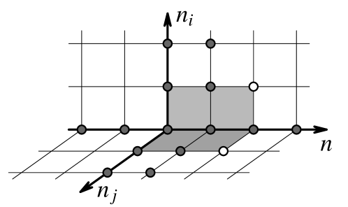
Figure 1: Pair of equations (8), $m=2$. Initial data are marked with the dark discs.

For a moment, it is convenient to identify the reference point $\mathbf{n}$ on the lattice with the origin $(0,0,0)$. The values $v^{i}_{s}=v(1,0,s)$, $v^{j}_{s}=v(0,1,s)$ are computed from the initial data according to equations (8). In order to find the values $v^{ij}_{s}=v(1,1,s)$, we have to solve the infinite set of equations

$$Q^{(i)}(v^{ij}_{s+m},\dots,v^{ij}_{s},v^{j}_{s+m},\dots,v^{j}_{s})=0,$$ (9)

$$Q^{(j)}(v^{ij}_{s+m},\dots,v^{ij}_{s},v^{i}_{s+m},\dots,v^{i}_{s})=0,\quad s\in\mathbb{Z}.$$

Taking $s=m-1,\dots,0$, we get a system of $2m$ equations for $2m$ unknowns $v^{ij}_{2m-1},\dots,v^{ij}$. We will assume that functions $Q^{(i)},Q^{(j)}$ are generic in the sense that this system is not degenerate and possesses a finite set of solutions. However, this does not guarantee that a solution exists for the whole set of equations (9). Indeed, if we consider additionally $s=m$ then two new equations for a single new unknown $v^{ij}_{2m}$ are added, which, generally, do not admit a solution in common. We are interested in the special type of equations such that a solution of system (9) exists for the generic initial data.

Notice that expressions for $v^{ij}_{m-1},\dots,v^{ij}$ as functions of initial data can contain only

$$v_{m-1},\dots,v,\quad v^{i}_{m-1},\dots,v^{i},\quad v^{j}_{m-1},\dots,v^{j}.$$

Indeed, since $v^{ij}_{m-1},\dots,v^{ij}$ are found by solving equations (9) at $s=m-1,\dots,0$, hence these variables do not depend on $v_{s}$ at $s<0$. Similarly, these variables can be found by solving equations (9) at $s=-1,\dots,-m$, and this implies that there are no dependence on $v_{s}$ at $s>m-1$, as well. Therefore, if equations (8) are consistent then a mapping

$$R^{(ij)}:~{}(V^{i},V^{j},V)\to V^{ij},\quad V=(v_{m-1},\dots,v)$$

appears, which can be interpreted as a $m$-component quad-equation on the sublattice $(n_{i},n_{j})$. We derived it in the origin of the lattice, but it is clear that this mapping is defined at any point $\mathbf{n}$.

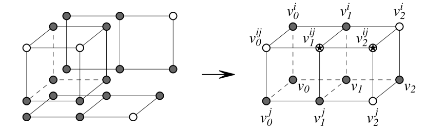
Figure 2: 3D-consistency for a pair of 2-quad-equations and a 2-component quad-equation. Dark disks correspond to the initial data; the stars mark the points where the consistency conditions are tested.

This observation brings to the desired formulation of the consistency conditions. In the following Definition, equations (8) are taken in the resolved form (6) (so that the solution of the 3D-consistent system is constructed in the octant $n_{i}\geq 0$, $n_{j}\geq 0$, $n\geq 0$). The components of the mapping $R^{(ij)}$ are enumerated by a subscript put in the square brackets in order to distinguish it from the shift with respect to $n$. The consistency condition on the 3-dimensional lattice is given in part (i) of the definition (fig. 2 illustrates it for $m=2$). In the multidimensional case, this condition must be satisfied on the sublattices $(n_{i},n_{j},n)$ for all $i,j$. The mappings $R^{(ij)}$ defined on all sublattices $(n_{i},n_{j})$ must satisfy the usual 3D-consistency condition for quad-equations on the sublattices $(n_{i},n_{j},n_{k})$, as stated in the part (ii).

Definition 1.

Let $V=(v_{m-1},\dots,v)$, $R^{(ij)}=(r^{(ij)}_{[m-1]},\dots,r^{(ij)}_{[0]})$. The system of equations

$$v^{i}_{m}=q^{(i)}(v^{i}_{m-1},\dots,v^{i},v_{m},\dots,v)=q^{(i)}(V^{i},v_{m},V),$$ (10)

$$V^{ij}=R^{(ij)}(V^{i},V^{j},V),\quad i\neq j$$ (11)

is called multidimensionally consistent if the following properties are fulfilled:

(i) for any pair $i\neq j$, the relations

$$\begin{gathered}r^{(ij)}_{[s]}(V^{i}_{1},V^{j}_{1},V_{1})=r^{(ij)}_{[s+1]}(V^{i},V^{j},V),\quad s=0,\dots,m-2,\\ r^{(ij)}_{[m-1]}(V^{i}_{1},V^{j}_{1},V_{1})=q^{(i)}(V^{ij},v^{j}_{m},V^{j})=q^{(j)}(V^{ij},v^{i}_{m},V^{i})\end{gathered}$$ (12)

where $v^{i}_{m}$, $v^{j}_{m}$, $V^{ij}$ are substituted from (10), (11), hold identically with respect to $v_{m},V$, $V^{i}$, $V^{j}$;

(ii) for any triple $i\neq j\neq k\neq i$, the relations

$$R^{(jk)}(V^{ij},V^{ik},V^{i})=R^{(ik)}(V^{ij},V^{jk},V^{j})=R^{(ij)}(V^{ik},V^{jk},V^{k})$$ (13)

where $V^{ij},V^{ik},V^{jk}$ are substituted from (11), hold identically with respect to $V,V^{i},V^{j},V^{k}$. ∎

Less formally, the identities (12), (13) can be represented as

$$v^{ij}_{1}=T(r^{(ij)}_{[0]})=r^{(ij)}_{[1]},\quad\dots,\quad v^{ij}_{m-1}=T(r^{(ij)}_{[m-2]})=r^{(ij)}_{[m-1]},$$

$$v^{ij}_{m}=T(r^{(ij)}_{[m-1]})=T_{j}(q^{(i)})=T_{i}(q^{(j)}),$$

$$V^{ijk}=T_{i}(R^{(jk)})=T_{j}(R^{(ik)})=T_{k}(R^{(ij)})$$

where it is assumed that the shift operators $T,T_{i},T_{j}$ act in virtue of equations (10), (11).

One can prove that these conditions are not only necessary, but also sufficient, on a lattice of arbitrary dimension, for the existence of common solution of equations (10), (11) satisfying the generic initial data defined on all 2-dimensional coordinate sublattices $(\dots,0,n_{i},0,\dots,0,n)$.

Two examples of multidimensionally consistent systems are presented in the rest sections.

3 Bäcklund transformation for the Bogoyavlensky lattice

There are several discrete equations of type (5) related to the Bogoyavlensky lattice

$$\partial_{t}u=u(u_{m}+\dots+u_{1}-u_{-1}-\dots-u_{-m})$$ (14)

and its modified versions. We restrict ourselves by consideration of just one such equation which defines the Bäcklund transformation for the lattice (14) in a potential form. The goal of this section is to prove the property of multidimensional consistency, as formulated in the following theorem, and to demonstrate that it is equivalent to the permutability property of the Bäcklund transformations.

Theorem 1.

The system consisting of $m$-quad-equations

$$(v_{m}-v^{i}_{m})\cdots(v-v^{i})=\beta^{(i)}v_{m-1}\cdots vv^{i}$$ (15)

and of $m$-component quad-equations

$$v^{ij}=\frac{\beta^{(j)}P^{(i)}v^{j}-\beta^{(i)}P^{(j)}v^{i}}{\beta^{(j)}P^{(i)}-\beta^{(i)}P^{(j)}},\quad P^{(i)}:=(v_{m-1}-v^{i}_{m-1})\dots(v-v^{i}),$$ (16)

$$\frac{v^{ij}_{s}-v^{j}_{s}}{v^{j}_{s-1}}+\frac{v^{j}_{s}-v^{i}_{s}}{v_{s-1}}+\frac{v^{i}_{s}-v^{ij}_{s}}{v^{i}_{s-1}}=0,\quad s=1,\dots,m-1$$ (17)

is multidimensionally consistent in the sense of Definition 1. Also, it is consistent with the lattice equation

$$\partial_{t}v=v\left(\frac{v_{m}}{v}+\frac{v_{m-1}}{v_{-1}}+\cdots+\frac{v}{v_{-m}}\right)$$ (18)

related with (14) by the substitution $u=v_{m}/v$.

In particular, at $m=1$ (the Volterra lattice case), equation (15) takes the form

$$(v_{1}-v^{i}_{1})(v-v^{i})=\beta^{(i)}vv^{i}$$

and system (16), (17) is reduced to the quad-equation $Q^{0}_{1}$

$$\beta^{(i)}(v-v^{j})(v^{i}-v^{ij})=\beta^{(j)}(v-v^{i})(v^{j}-v^{ij}).$$

In the general case, equation (17) without the restrictions on the values of $s$ is a well-known 3-dimensional integrable equation equivalent to the Hirota equation. The multidimensional consistency property for equations of this type was studied in [26]. Equation (16) is a constraint which defines a reduction of this 3-dimensional equation to the $m$-component 2-dimensional one and equations (15) play the role of additional constraints. One proof of the theorem can be obtained by verifying the compatibility of these constraints with the 3-dimensional equation.

We will take another way which is completely within the 2-dimensional theory, starting from the Darboux transformation for the discrete linear problem

$$\psi_{-1}-u\psi_{m}=\lambda\psi$$ (19)

associated with the Bogoyavlensky lattice.

Statement 2.

Let the function $\psi(n)$ be a solution of equation (19) where

$$u=f_{m}\cdots f_{1}(f-\alpha)$$ (20)

and $u(n)\neq 0$ for all $n$, then the function

$$\tilde{\psi}=\frac{1}{f-\alpha}\Bigl{(}\frac{\alpha}{\lambda}\psi_{-1}-f\psi\Bigr{)}$$ (21)

is a solution of equation $\tilde{\psi}_{-1}-\tilde{u}\tilde{\psi}_{m}=\lambda\tilde{\psi}$ where

$$\tilde{u}=(f_{m}-\alpha)f_{m-1}\cdots f.$$ (22)

Proof.

It is easy to prove that if $u,\tilde{u}$ are of the prescribed form then the operators

$$L=T^{-1}-uT^{m},\quad\tilde{L}=T^{-1}-\tilde{u}T^{m},\quad A=\frac{1}{f-\alpha}\Bigl{(}\frac{\alpha}{\lambda}T^{-1}-f\Bigr{)},$$

$$B=\frac{\lambda}{\alpha}+\frac{\alpha^{m-1}}{\lambda^{m-1}}(f-\alpha)T(1-Y^{m})(1-Y)^{-1}$$

where

$$Y=\frac{\lambda}{\alpha}fT,\quad\mu=\frac{\alpha^{m}}{\lambda^{m}}-\frac{\lambda}{\alpha}$$

satisfy the identities

$$B\cdot(f-\alpha)A=L-\lambda+\mu(f-\alpha),$$

$$(f-\alpha)A\frac{1}{f-\alpha}B\cdot(f-\alpha)=\tilde{L}-\lambda+\mu(f-\alpha).$$

Here, we assume that $\alpha\neq 0$ since otherwise the statement becomes trivial. In order to make the computation, it is convenient to represent the operator $A$ as $A=\dfrac{\alpha}{\lambda(f-\alpha)}(1-Y)T^{-1}$.

The first identity implies that any solution of equation $L\psi=\lambda\psi$ satisfies as well the equation

$$B\cdot(f-\alpha)A\psi=\mu(f-\alpha)\psi.$$

Hence, $\tilde{\psi}=A\psi$ satisfies the equation

$$A\frac{1}{f-\alpha}B\cdot(f-\alpha)\tilde{\psi}=\mu\tilde{\psi}$$

and the second identity implies $\tilde{L}\psi=\lambda\tilde{\psi}$. ∎

Remark 1.

The condition $u(n)\neq 0$ means, apparently, that $f(n)\neq 0$, $f(n)\neq\alpha$, for all $n$. In principle, this restriction may be waived, but it does not lead to an essential generalization, rather it requires a lot of stipulations. So, we will assume that this condition is fulfilled in what follows.

Relations (20), (22) play the role of the Miura type transformations for the Bogoyavlensky lattice. Given the function $u$, any function $f$ satisfying the equation $u=f_{m}\cdots f_{1}(f-\alpha)$ can be represented as $f=\phi_{-1}/\phi$ where $\phi$ is a particular solution of equation (19) at $\lambda=\alpha$. The lattice (14) is equivalent to the compatibility condition of equation (19) and

$$\partial_{t}\psi=\psi_{-m-1}-(u+\cdots+u_{-m})\psi$$

and this allows to obtain easily the modified lattice equation for the variable $f$:

$$\partial_{t}f=f(f-\alpha)(f_{m}\cdots f_{1}-f_{-1}\cdots f_{-m}).$$ (23)

Vice versa, a direct computation proves that each of the substitutions (20), (22) maps solutions of equation (23) into solutions of equation (14). The elimination of the variable $u$ brings to the following statement.

Statement 3.

Equation

$$(f_{m}-\alpha)f_{m-1}\cdots f=\tilde{f}_{m}\cdots\tilde{f}_{1}(\tilde{f}-\tilde{\alpha})$$ (24)

defines the $n$-part of the Bäcklund transformation for equation (23), that is, differentiating of (24) in virtue of (23) and an analogous lattice equation for $\tilde{f},\tilde{\alpha}$ yields a relation which holds identically in virtue of equation (24) itself.

In other words, the lattice equation (23) defines a higher symmetry for (24). The existence of just one such symmetry is a nontrivial fact which allows to say about the integrability of the equation. But, what is about the 3D-consistency? As we have already mentioned in the introduction, although (24) belongs to the class of equations (5) under consideration, but the variables $f$ are naturally associated with the edges of the lattice rather than the vertices, and the Definition from the previous section is not suitable. In this situation, the 3D-consistency should be understood in the sense of the Yang–Baxter maps. We do not give one more general definition, since the variables $f$ play an auxiliary role in our consideration; the required property is formulated in Statement 4 below. In order to prove it, we use the matrix representation of the linear problem (19) and its Darboux transformation (21)

$$\Psi_{-1}=U\Psi,\quad\widetilde{\Psi}=F\Psi\quad\Rightarrow\quad\widetilde{U}F=F_{-1}U$$ (25)

where $\Psi$ is a $(m+1)$-dimensional vector and $U,F$ are $(m+1)\times(m+1)$ matrices:

$$\Psi=\begin{pmatrix}\psi_{m}\\ \vdots\\ \psi\end{pmatrix},\quad U=\begin{pmatrix}0&1&\dots&0\\ &&\ddots&\\ 0&0&\dots&1\\ u&0&\dots&\lambda\end{pmatrix},$$ (26)

$$F=\begin{pmatrix}-\frac{f_{m}}{f_{m}-\alpha}&\frac{\alpha}{\lambda(f_{m}-\alpha)}&0&\dots&0\\ 0&-\frac{f_{m-1}}{f_{m-1}-\alpha}&\frac{\alpha}{\lambda(f_{m-1}-\alpha)}&\dots&0\\ &&\ddots&\ddots&\\ 0&0&\dots&-\frac{f_{1}}{f_{1}-\alpha}&\frac{\alpha}{\lambda(f_{1}-\alpha)}\\ \frac{\alpha}{\lambda}f_{m}\cdots f_{1}&0&\dots&0&-1\end{pmatrix}.$$ (27)

These matrices are easily derived from equations (19), (21). Statement 2 means exactly that relations (20)–(22) are equivalent to the matrix equations (25). The permutability property of two Darboux transformations of this form

$$\widetilde{\Psi}=F[f,\alpha,\lambda]\Psi,\quad\widehat{\Psi}=F[g,\beta,\lambda]\Psi$$

is expressed by equation

$$F[\tilde{g},\beta,\lambda]\,F[f,\alpha,\lambda]=F[\hat{f},\alpha,\lambda]\,F[g,\beta,\lambda].$$ (28)

Due to the special structure of the matrices this equation can be easily solved and a direct computation brings to the following statement. The proof scheme of the identity (30) based on the refactorization of the product of matrix triple is well known (see e.g. [27]).

Statement 4.

Let matrices $F$ be of the form (27) and $\alpha\neq\beta$ then equation (28), viewed as an identity with respect to $\lambda$, is uniquely solved with respect to $\hat{f},\tilde{g}$ for the generic values of $f,g$. Denote $f=f^{(i)}$, $\alpha=\alpha^{(i)}$, $g=f^{(j)}$, $\beta=\alpha^{(i)}$, then the solution is written as the $m$-component mapping

$$T_{j}(f^{(i)}_{1})=\frac{(\alpha^{(j)}f^{(j)}_{m}\cdots f^{(j)}_{1}-\alpha^{(i)}f^{(i)}_{m}\cdots f^{(i)}_{1})(f^{(j)}_{1}-\alpha^{(j)})}{f^{(i)}_{m}\cdots f^{(i)}_{2}(\alpha^{(j)}f^{(i)}_{1}-\alpha^{(i)}f^{(j)}_{1})},$$ (29)

$$T_{j}(f^{(i)}_{s})=\frac{f^{(i)}_{s}(f^{(j)}_{s}-\alpha^{(j)})(\alpha^{(j)}f^{(i)}_{s-1}-\alpha^{(i)}f^{(j)}_{s-1})}{(f^{(j)}_{s-1}-\alpha^{(j)})(\alpha^{(j)}f^{(i)}_{s}-\alpha^{(i)}f^{(j)}_{s})},\quad s=2,\dots,m.$$

This mapping satisfies the 3D-consistency property

$$T_{k}T_{j}(f^{(i)}_{s})=T_{j}T_{k}(f^{(i)}_{s}),\quad s=1,\dots,m.$$ (30)

Proof.

One can prove that equation (28) is uniquely solvable also with respect to the variables $\hat{f},g$, for given $\tilde{g},f$. Moreover, the following property is fulfilled: if parameters $\alpha,\beta,\gamma$ are distinct and

$$F[h,\gamma,\lambda]F[g,\beta,\lambda]F[f,\alpha,\lambda]=F[h^{\prime},\gamma,\lambda]F[g^{\prime},\beta,\lambda]F[f^{\prime},\alpha,\lambda]$$ (31)

then $h^{\prime}=h$, $g^{\prime}=g$, $f^{\prime}=f$. This follows from the fact that the matrix (27) is uniquely defined by its one-dimensional kernel at the spectral parameter value $\lambda=\alpha$:

$$\ker F[f,\alpha,\alpha]=(1,f_{m},f_{m}f_{m-1},\dots,f_{m}\cdots f_{1})^{\top}.$$

Now, let us assign the parameters $\alpha,\beta,\gamma$ to three coordinate directions and consider refactorizations of the matrix $F[h,\gamma,\lambda]F[g,\beta,\lambda]F[f,\alpha,\lambda]$ corresponding to all permutations of these parameters. Due to the property (31), each permutation corresponds to a unique set of values $f,g,h$ which are naturally associated with edges of a cube. Moreover, the value at each edge is obtained by two different sequences of pairwise refactorizations which is equivalent to the property (30). ∎

Proof of the Theorem 1.

The above statements imply the consistency, in the lattice of arbitrary dimension, of equations

$$u=f^{(i)}_{m}\cdots f^{(i)}_{1}(f^{(i)}-\alpha^{(i)}),\quad u^{i}=(f^{(i)}_{m}-\alpha^{(i)})f^{(i)}_{m-1}\cdots f^{(i)},$$ (32)

the mapping (29) and the differential-difference equations (14), (23). The final step is to pass from the edge-type variables $f^{(i)}$ to the variables $v$ associated with the vertices of the lattice. To do this, notice that (32) implies the multiplicative conservation law

$$\frac{u^{i}}{u}=\frac{(f^{(i)}_{m}-\alpha^{(i)})/f^{(i)}_{m}}{(f-\alpha)/f}$$ (33)

and this allows to introduce (uniquely up to a constant factor) the potential variable $v$, according to the equations

$$u=\frac{v_{m}}{v},\quad f^{(i)}=\frac{\alpha^{(i)}v}{v-v^{i}}.$$

Under this change, equations (14), (23) turn into equation (18), relations (32) turn into the $m$-quad-equation (15) and the mapping (29) turn into the $m$-component quad-equation (16), (17). The parameter $\alpha$ enters into new equations only in power of $m+1$, so we denote additionally $(\alpha^{(i)})^{m+1}=\beta^{(i)}$. ∎

Remark 2.

The potential can be introduced in different ways, for instance, instead of (33) one can consider the conservation law

$$\frac{u^{i}_{1}}{u}=\frac{f^{(i)}_{m+1}-\alpha^{(i)}}{f-\alpha}$$

which leads to the substitution

$$u=\frac{w_{m+1}}{w},\quad f^{(i)}=\frac{w^{i}_{1}}{w}+\alpha^{(i)}.$$

The variable $w$ satisfies the equation

$$w_{m}\cdots w=(w^{i}_{m}+\alpha^{(i)}w_{m-1})\cdots(w^{i}_{1}+\alpha^{(i)}w)w^{i}$$

with the properties similar to the properties of equation (15).

Remark 3.

From the point of view of logical simplicity, introducing of the potential seems to be a redundant step, because we already have the variable defined in the vertices of the lattice—this is $u$, the coefficient of the original linear problem (19). This variable satisfies some multiquad-equation, indeed, but the problem is that it is too complicated and it is hardly possible to write it down in general form for all $m$. In contrast to equations for $f$, $v$ or $w$, this equation is not affine-linear with respect to the involved values. For instance, in the simplest case $m=1$, the relations (20) take the form

$$u=f_{1}(f-\alpha),\quad\tilde{u}=(f_{1}-\alpha)f;$$

from here one finds

$$f=\frac{1}{2\alpha}(u-\tilde{u}+\alpha^{2}+\sqrt{(\tilde{u}-u)^{2}+2\alpha^{2}(\tilde{u}+u)+\alpha^{4}}),\quad f_{1}=f+\frac{1}{\alpha}(\tilde{u}-u)$$

and elimination of $f$ brings to the quad-equation

$$\quad\tilde{u}-u+\sqrt{(\tilde{u}-u)^{2}+2\alpha^{2}(\tilde{u}+u)+\alpha^{4}})\\ =u_{1}-\tilde{u}_{1}+\sqrt{(\tilde{u}_{1}-u_{1})^{2}+2\alpha^{2}(\tilde{u}_{1}+u_{1})+\alpha^{4}}).\quad$$

It can be brought to a polynomial form quadratic with respect to each variable; the general theory of such equations was developed in [28]. Analogously, at $m=2$, a polynomial equation cubic with respect to each variable appears after elimination of $f,\dots,f_{4}$ from equations

$$u_{s}=f_{s+2}f_{s+1}(f_{s}-\alpha),\quad\tilde{u}_{s}=(f_{s+2}-\alpha)f_{s+1}f_{s},\quad s=0,1,2.$$

4 Bäcklund transformation for the discretization of Sawada–Kotera equation

This section is devoted to the discrete equations related to the lattice equation

$$\partial_{t}u=u^{2}(u_{m}\cdots u_{1}-u_{-1}\cdots u_{-m})-u(u_{m-1}\cdots u_{1}-u_{-1}\cdots u_{1-m}).$$ (34)

The main result is the following Theorem, which presents the Bäcklund transformation and nonlinear superposition formula for the potential form of (34).

Theorem 5.

The following system of equations is multidimensionally consistent:

$$(v^{i}_{m}-v)v^{i}_{m-1}\cdots v^{i}=\alpha^{(i)}(v_{m}-v^{i})v_{m-1}\cdots v,$$ (35)

$$v^{ij}_{s}=v_{s}\frac{P^{(i,j)}_{s+1}}{P^{(i,j)}_{s}},\quad s=0,\dots,m-1$$ (36)

where

$$\begin{aligned} P^{(i,j)}_{s}&=(\alpha^{(i)}v^{j}_{m-1}\cdots v^{j}-\alpha^{(j)}v^{i}_{m-1}\cdots v^{i})v_{m-1}\cdots v\\ &\quad+\sum^{m-1}_{r=0}\gamma^{(i,j)}_{r,s}(v_{m-1}\cdots v_{r+1})^{2}v_{r}(v^{i}_{r}-v^{j}_{r})v^{i}_{r-1}\cdots v^{i}v^{j}_{r-1}\cdots v^{j},\end{aligned}$$

$$\gamma^{(i,j)}_{r,s}=\begin{cases}1&s\leq r,\\ \alpha^{(i)}\alpha^{(j)}&r<s.\end{cases}$$

It is also consistent with the lattice equation

$$\partial_{t}v=\frac{v_{m-1}\cdots v}{v_{-1}\cdots v_{-m}}(v_{m}-v_{-m})$$ (37)

related with (34) by the substitution $u=v_{m}/v$.

Notice, that equation (34) at $m=1$ coincides with the modified Volterra lattice $\partial_{t}u=u^{2}(u_{1}-u_{-1})$ and system (36) turns into equation

$$(\alpha^{(i)}-1)(v^{ij}v^{j}-\alpha^{(j)}v^{i}v)=(\alpha^{(j)}-1)(v^{ij}v^{i}-\alpha^{(i)}v^{j}v)$$

which is equivalent to $H^{0}_{3}$ quad-equation. Equation (34) at $m>1$ was studied in [20], where it was shown that its continuous limit coincides with the Sawada–Kotera equation. This equation contains, as particular cases, the modified Bogoyavlensky lattices

$$\partial_{t^{\prime}}u=u^{2}(u_{m}\cdots u_{1}-u_{-1}\cdots u_{-m}),\quad\partial_{t^{\prime\prime}}u=u(u_{m-1}\cdots u_{1}-u_{-1}\cdots u_{1-m})$$

which can be obtained by scaling $u,t$ and passing to the limit. However, these flows do not commute and the integrability of their linear combination is a nontrivial fact which follows from the existence of the Lax pair [20]

$$u\psi_{m+1}-\psi_{m}+\lambda(\psi_{1}-u\psi)=0,$$ (38)

$$\partial_{t}\psi=u_{-1}\cdots u_{-m}(\lambda\psi_{-m}-\lambda^{-1}\psi_{m}).$$ (39)

It is easy to verify that equation (34) is equivalent to the compatibility condition for these linear equations.

Derivation of the Darboux transformation for equation (38) is the main step in the proof of Theorem 5. The action of this transformation on function $\psi$ is defined in a more complicated way than in the case of the Bogoyavlensky lattice, where operators of the first order were used (see Statement 2). Nevertheless, on the level of coefficients of the linear problem the Darboux transformation is described, as before, by the pair of Miura type substitutions,

$$u=\frac{g}{G}f,\quad\tilde{u}=\frac{g}{G}f_{m}$$ (40)

where

$$g=f_{m-1}\cdots f_{1}-\alpha,\quad G=f_{m}\cdots f-\alpha$$

(this notation will be used throughout the section).

Statement 6.

Let functions $u,\tilde{u}$ be of the form (40), $\psi$ be a solution of equation (38) and $\tilde{\psi}$ be a solution of similar equation

$$\tilde{u}\tilde{\psi}_{m+1}-\tilde{\psi}_{m}+\lambda(\tilde{\psi}_{1}-\tilde{u}\tilde{\psi})=0.$$ (41)

Then both formulae $\chi=\psi_{1}-f\psi$ and $\chi=\tilde{\psi}-f\tilde{\psi}_{1}$ define a solution of equation

$$(1-f_{m}f)(f_{1}g_{1}\chi_{m+1}+\lambda G_{1}\chi_{1})=(1-f_{m+1}f_{1})(G\chi_{m}+\lambda f_{m}g\chi).$$ (42)

Proof.

Let us consider the first substitution:

$$\chi=\psi_{1}-f\psi,$$

$$\chi_{1}=\psi_{2}-f_{1}\psi_{1},$$

$$\chi_{m}=\psi_{m+1}-f_{m}\psi_{m}=\lambda\psi-\frac{\lambda}{u}\psi_{1}+\Bigl{(}\frac{1}{u}-f_{m}\Bigr{)}\psi_{m},$$

$$\chi_{m+1}=\lambda\psi_{1}-\frac{\lambda}{u_{1}}\psi_{2}+\Bigl{(}\frac{1}{u_{1}}-f_{m+1}\Bigr{)}(\chi_{m}+f_{m}\psi_{m}).$$

Equation for $\chi$ is obtained by solving first three equations with respect to $\psi_{1},\psi_{2},\psi_{m}$ and plugging the result into the last one. A straightforward (but rather lengthy) computation proves that the terms with $\psi$ cancel out (taking the relation $u=gf/G$ into account) and equation (42) appears.

The second substitution $\chi=\tilde{\psi}-f\tilde{\psi}_{1}$ can be checked analogously, but it is better to make use of the reflection

$$f(n)\to f(-n),\quad\psi(n)\leftrightarrow\tilde{\psi}(1-n),\quad\chi(n)\to\chi(-n),\quad\lambda\to\frac{1}{\lambda}.$$

Under this transformation, equations (38) and (41) turn into each other, as well as the substitutions $\chi=\psi_{1}-f\psi$ and $\chi=\tilde{\psi}-f\tilde{\psi}_{1}$, and equation (42) does not change. Indeed, equation (38)

$$\frac{f_{m-1}\cdots f_{1}-\alpha}{f_{m}\cdots f-\alpha}f(\psi_{m+1}-\lambda\psi)=\psi_{m}-\lambda\psi_{1}$$

turns into

$$\frac{f_{-m+1}\cdots f_{-1}-\alpha}{f_{-m}\cdots f-\alpha}f(\tilde{\psi}_{-m}-\frac{1}{\lambda}\tilde{\psi}_{1})=\tilde{\psi}_{1-m}-\frac{1}{\lambda}\tilde{\psi}$$

and applying of $-\lambda T^{m}$ results in equation (41)

$$\frac{f_{m-1}\cdots f_{1}-\alpha}{f_{m}\cdots f-\alpha}f_{m}(\tilde{\psi}_{m+1}-\lambda\tilde{\psi})=\tilde{\psi}_{m}-\lambda\tilde{\psi}_{1}.$$

To verify the invariance of equation (42), it is sufficient to notice that the reflection sends $g_{k}$ to $g_{-m-k}$ and $G_{k}$ to $G_{-m-k}$. ∎

Equation (42) looks awkward, but we need it only as an intermediate between equations (38) and (41). It is important only that both these equations admit first order Darboux transformations into one and the same equation, so it is possible to define a Darboux transformation between them:

$$\chi=(T-f)\psi,\quad\chi=(1-fT)\tilde{\psi}\quad\Rightarrow\quad\tilde{\psi}=(1-fT)^{-1}(T-f)\psi.$$

The operator $1-fT$ is invertible in virtue of equation (38) and the operator $(1-fT)^{-1}(T-f)$ is equivalent to some operator of $m$-th order (its explicit form is rather bulky, but we do not need it). In the matrix representation, the Darboux transformation is defined by equations

$$\Psi_{1}=U\Psi,\quad\tilde{\Psi}=F\Psi,\quad F=B^{-1}A$$

where

$$\Psi=\begin{pmatrix}\psi\\ \vdots\\ \psi_{m}\end{pmatrix},\quad U=\begin{pmatrix}0&1&\dots&0&0\\ 0&0&\ddots&0&0\\ &&\ddots&\ddots&\\ 0&0&\dots&0&1\\ \lambda&-\dfrac{\lambda}{u}&\dots&0&\dfrac{1}{u}\end{pmatrix},$$

$$A=\begin{pmatrix}-f&1&\dots&0&0\\ 0&-f_{1}&\ddots&0&0\\ &&\ddots&\ddots&\\ 0&0&\dots&-f_{m-1}&1\\ \lambda&-\dfrac{\lambda G}{gf}&\dots&0&\dfrac{G}{gf}-f_{m}\end{pmatrix},$$ (43)

$$B=\begin{pmatrix}1&-f&\dots&0&0\\ 0&1&\ddots&0&0\\ &&\ddots&\ddots&\\ 0&0&\dots&1&-f_{m-1}\\ -\lambda f_{m}&\lambda\dfrac{G}{g}&\dots&0&1-\dfrac{G}{g}\end{pmatrix}.$$ (44)

The consistency condition $\widetilde{U}F=F_{1}U$ is exactly equivalent to the relations (40). Pay attention that although the variable $f_{m}$ enters the matrices $A$ and $B$, the matrix $F$ does not depend on it.

A more complicated structure of the Darboux matrix $F$ is the only essential difference from the example considered in the previous section. The general scheme of the proof remains the same. Any function $f$ satisfying equation $u=gf/G$ can be represented as $f=\phi_{1}/\phi$ where $\phi$ is a particular solution of equation (38) at $\lambda=\alpha$. The use of equation (39) brings to the modified lattice equation

$$\partial_{t}f=f\frac{g_{-1}\cdots g_{-m+1}}{G\cdots G_{-m}}\bigl{(}gg_{-m}(G-G_{-m})-GG_{-m}(g-g_{-m})\bigr{)}.$$ (45)

Vice versa, one can verify intermediately that each substitution (40) maps a solution of equation (45) into a solution of (34). This proves the following statement.

Statement 7.

Equation

$$\frac{(\tilde{f}_{m-1}\cdots\tilde{f}_{1}-\tilde{\alpha})\tilde{f}}{\tilde{f}_{m}\cdots\tilde{f}-\tilde{\alpha}}=\frac{f_{m}(f_{m-1}\cdots f_{1}-\alpha)}{f_{m}\cdots f-\alpha}$$ (46)

defines the $n$-part of the Bäcklund transformation for equation (45), that is, the relation obtained by differentiating of this equation in virtue of (45) and a similar lattice equation for $\tilde{f},\tilde{\alpha}$ is fulfilled identically in virtue of the equation itself.

Remark 4.

An interesting property of equation (46) at $\tilde{\alpha}=\alpha$ is that it admits a reduction to an equation of order $m-1$. More precisely, one can prove that it can be brought to the form $\tilde{f}T(Q)=f_{m}Q$ where $Q$ is a polynomial depending on $f,\dots,f_{m-1},\tilde{f},\dots,\tilde{f}_{m-1}$, so that equation $Q=0$ defines a special solution of (46). Moreover, equation $Q=0$ is also consistent with the lattice equation (45). For instance, in the simplest case $m=2$, the quad-equation appears (a discrete analog of the Tzitzeica equation)

$$\tilde{f}f_{1}(\alpha^{-1}\tilde{f}_{1}f-\tilde{f}_{1}-f)+f_{1}+\tilde{f}-\alpha=0$$

which is consistent with the flow

$$\partial_{t}f=\frac{f(f-\alpha)}{f_{1}ff_{-1}-\alpha}\left(\frac{f(f_{1}-\alpha)(f_{-1}-\alpha)(f_{2}f_{1}-f_{-1}f_{-2})}{(f_{2}f_{1}f-\alpha)(ff_{-1}f_{-2}-\alpha)}-f_{1}+f_{-1}\right).$$

Equation (24) admits an analogous lowering of the order.

Refactorization of the above Darboux matrices is a rather difficult task. Nevertheless, it is possible to write the general answer for arbitrary $m$ and we arrive to the following statement. The proof of 3D-consistency follows from the same general arguments as in the case of Statement 4.

Statement 8.

Let $F[f,\alpha,\lambda]=B^{-1}A$ where $A,B$ are matrices of the form (43), (44) and $\alpha^{(i)}\neq\alpha^{(j)}$. Then equation

$$F[T_{i}(f^{(j)}),\alpha^{(j)},\lambda]\,F[f^{(i)},\alpha^{(i)},\lambda]=F[T_{j}(f^{(i)}),\alpha^{(i)},\lambda]\,F[f^{(j)},\alpha^{(j)},\lambda]$$

considered as an identity with respect to $\lambda$ is uniquely solved with respect to $T_{i}(f^{(j)}),T_{j}(f^{(i)})$, for generic values of $f^{(i)}$, $f^{(j)}$. This gives rise to the $m$-component mapping

$$T_{j}(f^{(i)}_{s})=\frac{P^{(i,j)}_{s+1}}{f^{(j)}_{s}P^{(i,j)}_{s}},\quad s=0,\dots,m-1$$ (47)

where

$$\begin{aligned} P^{(i,j)}_{s}&=\alpha^{(i)}f^{(j)}_{m-1}\cdots f^{(j)}-\alpha^{(j)}f^{(i)}_{m-1}\cdots f^{(i)}\\ &\qquad+\sum^{m-1}_{r=0}\gamma^{(i,j)}_{r,s}(f^{(i)}_{r}-f^{(j)}_{r})f^{(i)}_{r-1}\cdots f^{(i)}f^{(j)}_{r-1}\cdots f^{(j)},\end{aligned}$$

$$\gamma^{(i,j)}_{r,s}=\begin{cases}1&s\leq r,\\ \alpha^{(i)}\alpha^{(j)}&r<s.\end{cases}$$

This mapping satisfies the 3D-consistency property

$$T_{k}T_{j}(f^{(i)}_{s})=T_{j}T_{k}(f^{(i)}_{s}),\quad s=0,\dots,m-1.$$

Now, the proof of Theorem 5 is obtained by introducing of the potential $v$ according to equations

$$u=\frac{v_{m}}{v},\quad f^{(i)}=\frac{v^{i}}{v}.$$

Under these substitutions, equations (40) turn into $m$-quad-equation (35), the mapping (47) turn into $m$-component quad-equation (36), and the lattice equations (34), (45) turn into equation (37). The consistency follows from the proven statements.

References

- [1] A.I. Bobenko, Yu.B. Suris. Integrable systems on quad-graphs. Int. Math. Res. Notices 2002:11 (2002) 573–611.
- [2] F.W. Nijhoff, A.J. Walker. The discrete and continuous Painlevé hierarchy and the Garnier system. Glasgow Math. J. 43A (2001) 109–123.
- [3] V.E. Adler, A.I. Bobenko, Yu.B. Suris. Classification of integrable equations on quad-graphs. The consistency approach. Commun. Math. Phys. 233 (2003) 513–543.
- [4] K. Narita. Soliton solution to extended Volterra equation. J. Phys. Soc. Japan 51:5 (1982) 1682–1685.
- [5] Y. Itoh. Integrals of a Lotka-Volterra system of odd number of variables. Progr. Theor. Phys. 78 (1987) 507–510.
- [6] O.I. Bogoyavlensky. Integrable discretizations of the KdV equation. Phys. Lett. A 134:1 (1988) 34–38.
- [7] S. Tsujimoto, R. Hirota, S. Oishi. An extension and discretization of Volterra equation I. Technical Report of IEICE, NLP92–90 (1993) 3pp.
- [8] V.G. Papageorgiou, F.W. Nijhoff. On some integrable discrete-time systems associated with the Bogoyavlensky lattices. Phys. A 228 (1996) 172–188.
- [9] Yu.B. Suris. Integrable discretizations of the Bogoyavlensky lattices. J. Math. Phys. 37 (1996) 3982–3996.
- [10] Yu.B. Suris. The problem of integrable discretization: Hamiltonian approach. Basel: Birkhäuser, 2003.
- [11] A. Fukuda, Y. Yamamoto, M. Iwasaki, E. Ishiwata, Y. Nakamura. A Bäcklund transformation between two integrable discrete hungry systems. Phys. Lett. A 375 (2011) 303–308.
- [12] R.I. Yamilov. On classification of discrete evolution equations. Usp. Mat. Nauk 38:6 (1983) 155–156 (in Russian).
- [13] R.I. Yamilov. Symmetries as integrability criteria for differential difference equations. J. Phys. A: Math. Theor. 39:45 (2006) R541–623.
- [14] D. Levi, M. Petrera, C. Scimiterna, R. Yamilov. On Miura transformations and Volterra-type equations associated with the Adler–Bobenko–Suris equations. SIGMA 4 (2008) 077 (14 pp).
- [15] D. Levi, R.I. Yamilov. The generalized symmetry method for discrete equations. J. Phys. A: Math. Theor. 42 (2009) 454012 (18pp).
- [16] D. Levi, R.I. Yamilov. Generalized symmetry integrability test for discrete equations on the square lattice. J. Phys. A: Math. Theor. (2011) 145207 (22pp).
- [17] R.N. Garifullin, E.V. Gudkova, I.T. Habibullin. Method for searching higher symmetries for quad-graph equations. J. Phys. A: Math. Theor. 44 (2011) 325202 (16pp).
- [18] R.N. Garifullin, R.I. Yamilov. Generalized symmetry classification of discrete equations of a class depending on twelve parameters. J. Phys. A: Math. Theor. 45 (2012) 345205 (23pp).
- [19] A.V. Mikhailov, J.P. Wang, P. Xenitidis. Cosymmetries and Nijenhuis recursion operators for difference equations. Nonlinearity 24 (2011) 2079–2097.
- [20] V.E. Adler, V.V. Postnikov. Differential-difference equations associated with the fractional Lax operators. J. Phys. A: Math. Theor. 44 (2011) 415203 (17pp).
- [21] A.P. Veselov, A.B. Shabat. Dressing chains and the spectral theory of the Schrödinger operators. Funct. Anal. Appl. 27:2 (1993) 81–96.
- [22] A.P. Veselov. Yang–Baxter maps and integrable dynamics. Phys. Lett. A 314:3 (2003) 214–221.
- [23] V.E. Adler, A.I. Bobenko, Yu.B. Suris. Geometry of Yang–Baxter maps: pencils of conics and quadrirational mappings. Comm. Anal. and Geom. 12:5 (2004) 967–1007.
- [24] V. Papageorgiou, A. Tongas, A. Veselov. Yang–Baxter maps and symmetries of integrable equations on quad-graphs. J. Math. Phys. 47:8 (2006) 083502.
- [25] V.G. Papageorgiou, A.G. Tongas. Yang–Baxter maps and multi-field integrable lattice equations. J. Phys. A: Math. Theor. 40:42 (2007) 12677–12690.
- [26] V.E. Adler, A.I. Bobenko, Yu.B. Suris. Classification of integrable discrete equations of octahedron type. Int. Math. Res. Notices 2012:8 (2012) 1822–1889.
- [27] V.E. Adler, R.I. Yamilov. Auto-transformations of integrable chains. J. Phys. A: Math. Gen. 27 (1994) 477–492.
- [28] J. Atkinson, M. Nieszporski. Multi-quadratic quad equations: integrable cases from a factorised-discriminant hypothesis. Int. Math. Res. Notices (2013) online.