PLUMED 2: New feathers for an old bird

Abstract

Enhancing sampling and analyzing simulations are central issues in molecular simulation. Recently, we introduced PLUMED, an open-source plug-in that provides some of the most popular molecular dynamics (MD) codes with implementations of a variety of different enhanced sampling algorithms and collective variables (CVs). The rapid changes in this field, in particular new directions in enhanced sampling and dimensionality reduction together with new hardwares, require a code that is more flexible and more efficient. We therefore present PLUMED 2 here - a complete rewrite of the code in an object-oriented programming language (C++). This new version introduces greater flexibility and greater modularity, which both extends its core capabilities and makes it far easier to add new methods and CVs. It also has a simpler interface with the MD engines and provides a single software library containing both tools and core facilities. Ultimately, the new code better serves the ever-growing community of users and contributors in coping with the new challenges arising in the field.

PROGRAM SUMMARY

Manuscript Title: PLUMED 2: New feathers for an old bird
Authors: Gareth A Tribello, Massimiliano Bonomi, Davide Branduardi, Carlo Camilloni and Giovanni Bussi
Program Title: PLUMED 2
Journal Reference:
Catalogue identifier:
Licensing provisions: Lesser GPL
Distribution format: tar.gz
Programming language: ANSI-C++
Computer: Any computer capable of running an executable produced by a C++ compiler
Operating system: Linux operative system, Unix OS-es
RAM: Depends on the number of atoms, the method chosen and the collective variables used
Number of processors used: 1 or more
Supplementary material: test suite, user and developer documentation, collection of patches, utilities
Classification: 3 Biology and Molecular Biology, 7.7 Other Condensed Matter inc. Simulation of Liquids and Solids, 23 Statistical Physics and Thermodynamics
External routines/libraries: GNU libmatheval, lapack
Nature of problem: calculation of free-energy surfaces for molecular systems of interest in biology, chemistry and materials science, on the fly and a-posteriori analysis of molecular dynamics trajectories using advanced collective variables
Solution method: implementations of various collective variables and enhanced sampling techniques
Unusual features: PLUMED 2 can be used either as standalone program, e.g. for a-posteriori analysis of trajectories, or as a library embedded in a Molecular Dynamics code (such as GROMACS, NAMD, Quantum ESPRESSO, and LAMMPS). Interface with these software is provided in a patch form. Library is documented to ease its embedding into other software.
Running time: Depends on the number of atoms, the method chosen and the collective variables used

1 Introduction

Molecular simulations are now regularly used to understand natural phenomena in a wide range of subjects, spanning from biochemistry to solid state physics. These techniques are used to complement and interpret the increasingly large amounts of data coming from experiments. These tools are useful because two major technical advancements make it so that it is now possible to extensively sample configuration space. The first of these is the Moore’s-law increase in computational power that has occurred during the last 50 years (see e.g. [1]). The second, perhaps more significant development, has been the creation of increasingly sophisticated algorithms [2, 3]. In the early days of simulations implementing new algorithms was straightforward as every group had their own custom molecular dynamics (MD) code. Nowadays, however, there are a number of algorithmically-advanced simulation suites [4, 5, 6, 7, 8, 9] that generally have a small number of technically-skilled developers and a much larger community of users. These codes are complex and carefully optimized to work on modern, parallel computer hardware, which is mandatory given the large computational facilities that are now available. However, this complexity makes experimenting and implementing new methods somewhat daunting. Moreover, new methods end up being implemented in a specific suite, which rapidly becomes obsolete thus further slowing their dissemination.

For the above reasons we introduced the PLUMED plug-in a few years ago [10]. This code was designed to “plug-in” to MD codes such as DL_POLY_CLASSIC [4], NAMD [6], GROMACS [7] and AMBER [9] and to extend them by providing a single implementation for free-energy methods such as umbrella sampling [11], metadynamics [12, 13] and steered MD [14]. It was hoped that PLUMED would encourage researchers in fields ranging from biophysics to solid-state physics to adopt these methods. Furthermore, given that the interface with the complex MD code was looked after deep within PLUMED and that the coding style of PLUMED was both simple and flexible, it was hoped that developers would use the code to share their methods with the widest possible community. PLUMED has been rather successful in both respects and the plug-in model has been adopted by other researchers [15]. To date there have been approximately 3200 downloads of PLUMED from our website, more than 150 articles in which the original PLUMED article has been cited, more than 200 users who have subscribed to our mailing list, and 20 different super users who have contributed code fragments to our repository. PLUMED can now be interfaced with 10 different MD codes and has even been used in ways we had not envisaged when the software was designed. Some particularly interesting developments being the use of PLUMED in at least three graphical tools that can be used to analyze trajectory data; namely, PLUMED GUI [16], METAGUI [17] and GISMO [18].

The original PLUMED code was not designed to work with such a large variety of different MD codes or to grow this rapidly. As a result maintaining the interfaces between PLUMED and the various MD codes has proved to be quite time-consuming. Furthermore, the lack of a developer manual and programming guidelines has discouraged some contributors from sharing their code fragments and has contributed to an untidy growth of the code.

Here we present PLUMED 2, a complete rewrite of the code aimed at addressing the weaknesses in the original design. In the new version, we have simplified considerably the interface between PLUMED and the MD codes so as to make this aspect of the code maintenance more straightforward. PLUMED is now compiled separately as a software library and is thus completely independent from the MD codes. We have also moved to a modern, object-oriented programming language (C++) so to take advantage of inheritance and polymorphism. This has enabled us to use a plug-in architecture with a general purpose core and functionality in separate modules. It is thus easier to write bug-resilient code that can be worked on by multiple developers at the same time. Furthermore, developers can now easily modify the code and in principle even release independent extensions thus bringing the PLUMED project closer to a community-based framework. In addition, the object-oriented style allows us to write reusable objects whose functions are described in a developer manual that is generated from the code. This makes it far easier to code the complex, multi-layered, nested collective variables (CVs) that are increasingly being used to perform dimensionality reduction [19]. Finally, the new code structure allows one to use the same code for both on-the-fly biasing/analysis and post-processing thus minimizing redundancy.

This paper is laid out as follows. We first describe the theoretical background to PLUMED 2 and the various possibilities that it offers (section 2). We then describe how the code works (section 3.1), the various standalone tools that form part of PLUMED (section 3.2) and the interface between a generic MD engine and PLUMED (section 3.2). We then provide a set of examples of varying complexity (section 4) before finishing by showing how straightforward it is to implement new features and speculating a little on the various ways that this new code could be used in the future (section 5).

2 Theoretical Background

In an MD simulation, the trajectories of a large number of atoms are calculated. The final result is thus a high dimensional description as to how the various atomic positions change as a function of time. It is very difficult to interpret the results of a simulation and to compare them with experimental data without further processing of the trajectory. A particularly useful way of processing the data is to calculate a histogram, $P(\mathbf{s})$, along a few selected CVs, $\mathbf{s}$, as from this one can calculate the free energy using:

$$F(\mathbf{s})=-k_{B}T\log(P(\mathbf{s})),$$ (1)

where $k_{B}$ is Boltzmann constant and $T$ is the temperature. This equation assumes that there are no high-energy barriers that prevent the system from visiting all the energetically-accessible portions of configuration space and that the trajectory is thus ergodic. Oftentimes this is not the case and a commonly used technique to deal with this so-called time-scale problem is to add a bias along one or multiple CVs and to thereby force the system to explore a wider range of CV values. In these methods (e.g. umbrella sampling, steered MD, metadynamics) the bias $V(\mathbf{X},t)$ takes the form of an external potential, which may or may not be time dependent, but that is always a function of some CVs, $\mathbf{s}(\mathbf{X})=\{s_{1}(\mathbf{X}),s_{2}(\mathbf{X}),\dots,s_{n}(\mathbf{X})\}$:

$$V(\mathbf{X},t)=V(s_{1}(\mathbf{X}),s_{2}(\mathbf{X}),\dots,s_{n}(\mathbf{X}),t).$$ (2)

A useful technique for providing greater flexibility in the code is to allow the user to construct new CVs as functions of other, simpler, CVs. Even with this complexity though, it is still straightforward to differentiate this potential and thus obtain the force the bias applies to the atoms using:

$$\frac{\partial V}{\partial x_{m}}=\sum_{i=1}^{n}\frac{\partial V}{\partial s_{i}}\frac{\partial s_{i}}{\partial x_{m}}.$$ (3)

This relation provides a powerful paradigm that can be used to design a flexible plug-in. The code can be divided into units that calculate the values and derivatives of the CVs, functions of CVs and biases in the equations above. The contribution the bias makes to the virial is calculated using a similar procedure but involving derivatives of collective variables with respect to the cell vectors. Obviously, there are inter-dependencies between these quantities - it is not possible to calculate the value of $V(\mathbf{X},t)$ without first calculating the CVs, $\mathbf{s}(\mathbf{X})$. Consequently, the various quantities must be calculated in an order that starts with those that have an explicit dependence on the atomic positions.

3 PLUMED 2 Overview

PLUMED 2 provides an executable and a C++ library. The most-basic function of both these tools is the calculation of CVs from the atomic positions. The benefit of having this functionality in a library as well as in a standalone executable is that this allows one to calculate CVs during an MD simulation. This use will become more and more important in the near future as the available computing power is increasing more rapidly than the volume of space that is available for storing trajectories. A second important function is PLUMED’s ability to add additional forces to the CVs as this is what allows us to implement free-energy methods such as umbrella sampling, steered MD and metadynamics. PLUMED can also be used to perform other forms of analysis of trajectory data. This can be done during post processing on the trajectory file, much like a conventional analysis tool, or on-the-fly during the simulation. Other software is available for analyzing existing trajectories [7, 20, 21, 22, 23, 24] or for biasing MD simulations [15, 9, 25, 26, 27, 7, 6]. PLUMED 2, however, is the only code we know of that allows users to do both sets of tasks with a single syntax. This is important as a number of recently-proposed algorithms [28, 29] use the results from an analysis of a relatively short MD simulation to refine the simulation bias.

PLUMED has now been completely redesigned to bring new features to both users and developers. Users will benefit from a new syntax for the input file that allows for much greater flexibility but which maintains strong similarities with the previous version. This flexibility can be exploited to create complex CVs without (or prior to) implementing them in C++. This is possible because the functionalities that are already available can be combined together directly from the input file. When this is done dependencies between quantities and chain rules for analytical derivatives are generated automatically. Users also benefit because PLUMED is now compiled independently from the underlying MD codes, which makes patching and including PLUMED in an MD engine considerably more straightforward. Lastly, virial contributions are calculated in PLUMED 2 so, unlike PLUMED 1, this code can be used to perform simulations with both constant temperature and constant pressure.

The PLUMED 2 code now has a modular organization centered on a kernel of core functionalities. This allows developers to more easily contribute additional features, such as new CVs and free-energy methods, as they do not have to edit the core code. Dynamic polymorphism is used to add those features in a concurrent manner or even at run time. This flexibility can be achieved by using C++ with minimal or no compromise on performance. In particular, many small utility classes are completely inlined, so as to obtain high level (i.e. easy to read) code running at maximum speed.

The PLUMED 2 executable can now also be used to run a few command-line tools. These tools allow the user to both analyze existing trajectories and to run simple MD simulations. In addition, there is an extensive set of regression tests. In these tests, PLUMED is used to analyze a set of trajectories and must reproduce exactly (within computational accuracy) a set of precomputed results. These tests can thus be used to ensure that new features are not introducing bugs into the software. Finally, the PLUMED 2 library contains several small utilities, such as classes for treating periodic boundary conditions, functions for calculating root-mean-square deviation from reference structures, and classes for editing and parsing strings. Developers are provided with extensive documentation that describes all these classes as we believe that many of them could be used in applications outside of the PLUMED project.

In the following, we discuss in more detail some of the most important features of PLUMED 2’s design. In particular, we will discuss the modularity of CVs and biasing methods, both from the points of view of a user and a developer, the use of PLUMED 2 from the command line as a standalone tool and the interface between PLUMED 2 and a generic MD engine.

3.1 How PLUMED 2 operates

This section explains how PLUMED 2 operates when it is used to analyze or bias MD simulations. PLUMED 2, much like the original PLUMED 1 package, takes a single dedicated input file in which each line instructs PLUMED to do something. An example input is shown below:

c1: COM ATOMS=1-10
c2: COM ATOMS=30-40
d1: DISTANCE ATOMS=c1,c2 COMPONENTS
a1: ANGLE ATOMS=14,15,16
f1: COMBINE ARG=d1.x,d1.y,d1.z POWERS=2,2,2
t1: TORSION ATOMS=20,c1,c2,23
b1: METAD ARG=f1,a1 PACE=20 HEIGHT=0.5 SIGMA=0.05,0.1
b2: UPPER_WALL ARG=d1.z AT=1.0 KAPPA=0.1
PRINT ARG=a1,t1,b1.bias,b2.bias FILE=colvar STRIDE=100

Each line in the input file above instructs PLUMED to create a new object, called an “Action”. Every conceivable thing the user instructs PLUMED to do be it the calculation of a CV (e.g. 

ISTANCE },
{\verb ANGLE } or {\verb TORSION } in the example) or a center of mass ({\verb COM }),
the writing out of some data ({\it e.g.}~{\verb PRINT } in the
above) or the calculation of a simulation bias ({\verb META

or

PPER_WALL }) can be cast as an Action object.  For the most part these Actions take in some input - usually either the positions of some of the atoms in
the system ({\it e.g.}~for the first center of mass in the above the input is the positions of atoms 1 through 10)  or the
instantaneous value of a CV - and use this data to calculate a new CV or bias potential.
Obviously, Actions cannot be performed in an arbitrary order as Actions that take CVs as input clearly
cannot be computed without first calculating the prerequisite CVs. Hence, PL

MED, while reading the input, ensures that the data required by each Action is either available without calculation from the trajectory or is part of the output from the Actions that precede it in the input file. The user should thus think of the PLUMED input file as a kind of primitive script that provides a set of instructions that will be executed during the simulation or during the analysis.

Most of the collective variables and methods that were available in PLUMED 1 can be recoded in PLUMED 2 using either a single Action or using a small number of Actions. Furthermore, the PLUMED 1 variables that have been recoded in PLUMED 2 contain fewer lines of executable code and many of them have a greater flexibility than their PLUMED 1 counterparts. At present we have reimplemented the basic geometric quantities (distances, angles and torsional angles) as well as quantities such as coordination numbers, minimum angles and alpha-beta similarities [30] that are non-linear combinations of these simpler quantities. We have also implemented the all important root-mean-square deviation [31] and have used these routines to write Actions to calculate the path CVs [32] and protein secondary structure variables [33] that were in PLUMED 1 and the generic property map that was recently proposed by Spiwok and Králová [34]. As well as these generic CVs PLUMED 2 contains implementations of CVs that are used by specific communities. For researchers examining polymers we have implemented the radius of gyration as well as inertia-tensors-based CVs [35]. Users can also calculate the total volume of the cell, the total potential energy of the system [36] or the dipole formed by a set of charged atoms. Lastly PLUMED 2 contains Actions for calculating the Debye-Hückel energy [37] and for interfacing PLUMED with the Almost library so that the CamShift Collective Variable [38, 39] can be calculated.

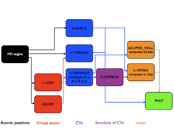
Figure 1: A diagram that shows how data is passed between the Actions in a PLUMED job.

Each of the Actions defined in the PLUMED input is given a unique label by the user. This label can be used to retrieve the output from the Action so that it can be used in a later part of the calculation. As an example of how this works in practice each of the first two commands in the input file above instructs PLUMED to calculate the position of a center of mass. These two centers of masses are stored in containers labeled 1 } and {\verb 2 and are used when PLUMED calculates the distance between center of mass 1 } and enter of mass 2 } as part of the Ation labeled

1 }.
 The first eight  Actions 

efined in the input above all do something similar - i.e. they all fill a container with the various quantities that are calculated during the Action’s execution. When only a single quantity is calculated this quantity is referenced in the later parts of the input file using the Action’s label. To reduce computational overhead some Actions calculate multiple quantities. The values output by these quantities can be referenced using $\langle$label$\rangle$.$\langle$component$\rangle$. As an example, the keyword OMPONENTS } in the DISTANE Action in the above instructs PLUMED to store the $x$, $y$ and $z$ components of the distances separately. These separate values can then be referenced using the labels 1.x }, {\verb 1.y and

1.z } as
they are above in the {\verb COMBINE } Action with label {\verb f1 }.  The
names of the quantities that are calculate

by any Action are provided in the manual and in the output at run-time so that the user can correctly refer to quantities when writing the input. Figure 1 illustrates the manner in which data is passed between Actions more clearly by showing schematically what quantities are calculated by each of the Actions in the above input and how this data is passed about.

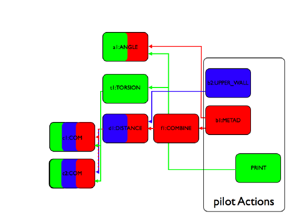
Figure 2: Schematic representation of how the Actions executed during each step of a PLUMED calculation are controlled by a small number of pilot Actions. The user specifies the frequencies with which these pilots should be performed. At each step PLUMED works out which pilots are to be performed and then activates all the Actions which calculate the data that is required by the active pilots.

The passing of data between the Actions in the input file introduces a clear set of interdependencies between them. This is illustrated for the input defined above in figure 2. As this figure shows, one cannot calculate the metadynamics bias without first calculating the function

1 } and the angle
{\verb a1 }. Similarly one need only calculate the torsion angle labeled {\verb t1 } during those steps when
the {\verb COLVAR } 

ile is written. PLUMED thus uses these interdependencies to control when the various Actions should be executed. The user provides instructions in the input as to the frequency with which certain, so called pilot Actions (in the example input above

ETAD }, {\verb UPPER_WALL } and {\verb PRINT } Actions) should be performed.
Then, when PLU

ED is called, it examines the list of pilot Actions, establishes which of them must be performed at the current time and activates the full set of Actions on which each of the active pilots depends. Once this process is completed PLUMED executes the set of activated Actions and calculates everything that is required at the current time step. This pre-screening of the Actions saves computational effort by ensuring that expensive CVs are only calculated when they are needed. It therefore considerably lowers the execution time for the calculation especially when expensive CVs are monitored only rarely.

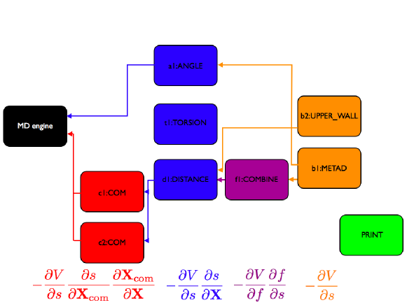
Figure 3: Figure showing how the forces from the simulation bias are transferred onto the atoms using the chain rule.

When one is using PLUMED to perform analysis on an MD trajectory, the calculation is finished once the values for each of the Actions has been calculated. By contrast when one is using PLUMED to bias the dynamics a second step is required as the forces from the bias must be transferred onto the atoms. This sort of calculation is possible because during the initial calculation step the derivatives of the CVs with respect to the input quantities are calculated as well as their values. As such the bias can be applied using the chain rule as is illustrated schematically for the input above in figure 3. During this final application step the code runs through the list of currently active Actions in reverse as it accumulates the forces on the atoms. These forces are ultimately passed back to the MD code and added to the forces from the interatomic potential. A special treatment is used for the NRGY CV [36]: instead of explicitly computing the derivatives, PLUMED takes advantage of the fact that the derivative of the potential energy is just minus the force.

PLUMED can also be used to implement multiple replica schemes such as parallel tempering metadynamics [40], multiple walkers metadynamics [41] and bias exchange metadynamics [30]. At present this can only be done using the GROMACS engine. However, the implementation is designed to be of general applicability and is based on the MPI library [42].

3.2 PLUMED 2 as a set of standalone tools

The simplest way to use PLUMED is to download the source from our website, compile it and then use it as a standalone tool. When PLUMED compiles it generates a single executable called

lumed }. This minimizes the number of clashes between PLUMED and
other 

rograms. Furthermore, a suffix can be added to the name of the executable so users can have multiple coexisting versions of PLUMED.

PLUMED’s command line tools are run by invoking the

lumed }
executable followed by the name of the tool of interest i.e. using the
following command:
%
\begin{verbatim}

lumed toolname A list of available tools can be retrieved using the command:

plumed help

All the command line tools share a similar syntax and a short help for a particular command can be obtained using the command:

plumed toolname --help

The PLUMED executable includes a simple Lennard-Jones MD code (implemd }) which can be ued to test the on-the-fly analysis and enhanced sampling algorithms, a tool called river } than can be use to analyze trajectories and a tool called um_hill that should be used to analyze the results from metadynamics simulations. It is straightforward to add further analysis programs as and when they are required. It is important to remember, however, that most of the code’s functionality can be explored using the

river } option.
\subsection{The interface with the MD co

e

One of the principal strengths of PLUMED is the ability to interface the plug-in with a variety of different MD, Monte Carlo and other modeling tools. This flexibility helps enormously when it comes to disseminating new techniques and also allows PLUMED to serve as a platform for cross validating different codes and methods.

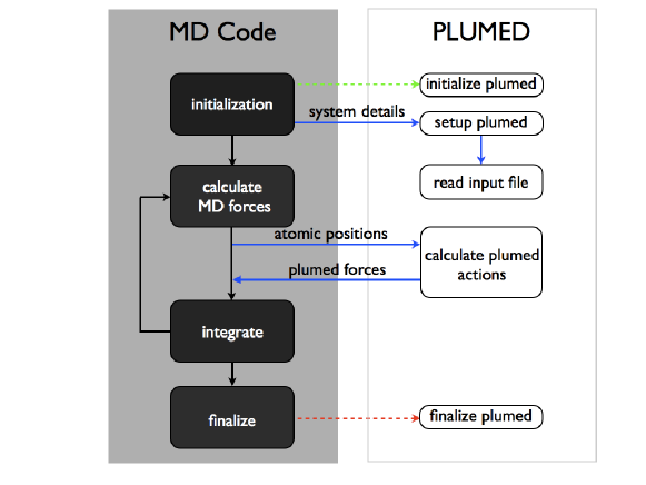
Figure 4: A schematic representation of the interface between PLUMED and an MD engine. The colors of the arrows indicate the particular PLUMED routine that the MD code should call to perform the task. Green arrows indicate a call to plumed_create, red arrows indicate a call to plumed_finalize and blue arrows indicate multiple calls to plumed_cmd.

PLUMED 1 was designed to compile at the same time as the underlying MD engine. This allowed us to reuse the underlying MD codes routines for calculating quantities such as distances, angles and torsions and their derivatives. However, it became problematic when implementing CVs and methods that were reliant on external libraries as to do this in a way that was transferable required one to modify the makefiles for all the MD codes supported by PLUMED - a laborious and largely thankless task. A consequence of this was that interfaces to the various codes grew at different rates and perhaps inevitably a bias was introduced towards those codes used by the majority of the developers. To resolve this, we decided that PLUMED 2 would have a single, standard interface, which is used with all the MD codes and which is not biased towards any particular package. The PLUMED routines that make up this interface serve only to communicate data between the MD code and PLUMED. This makes it possible to compile PLUMED as set of static object files, as a dynamic library and even as a standalone post-processing tool.

In spite of the changes in the way that it is compiled and linked to the MD engine the points where the MD engine calls PLUMED are the same as in the previous version. As shown in figure 4 PLUMED is called at three separate points in the MD code. The first is during initialization, the second occurs just after each force evaluation and the third is at the end of the simulation. Three PLUMED routines can be called from within the MD engine. The first of these routines initializes the code and creates the PLUMED object, while the last destroys the PLUMED object and frees the memory. The remaining routine is used in both the “setup plumed” and “calculate PLUMED Action” phases. It is a generic function that takes a character string and a void pointer as arguments. It is used to pass data between the MD engine and PLUMED. This mode of passing allows us to both retrieve data from the MD code and to modify the MD engine’s variables as is required for many biased MD methods. The simplicity of this interface makes it easy to reuse PLUMED in the many different MD engines used by the community. Furthermore, there is now some guarantee that the interface will continue to work when PLUMED is substituted by a different, future version. Most importantly, the guidelines for incorporating PLUMED into any MD engine are now very straightforward. In fact we have a step-by-step guide in the developer manual that explains how to incorporate PLUMED into any MD engine.

PLUMED’s simplified interface makes it much more straightforward to add the option to pass more data between the MD engine and PLUMED. For instance it would be relatively straightforward to add functionality to pass the atomic velocities from the MD engine to PLUMED. This opens the door to using PLUMED for many other methodologies and to a massive extension in the range of functionalities provided by PLUMED.

4 Examples

4.1 Steered MD on a system at the DFT level of theory

At heart PLUMED 2, like its predecessor, is a code for doing enhanced sampling calculations. Hence, in this first example we showcase these functionalities by demonstrating how we can use the plug-in to examine the SN2 reaction between a methyl-chloride molecule and a chlorine atom. The potential in this system was calculated using the BLYP density functional as implemented in the PW code from Quantum ESPRESSO 5.0 [8]. Obviously, the potential energy of the SN2 transition state is very high so we are unlikely to see the reaction in an unbiased MD simulation. To resolve this we used steered MD to force the reaction to occur. This method works by applying a harmonic potential, the equilibrium position of which moves at a constant velocity. In our SN2 reaction example this potential is a function of the distance between the carbon atom and one of the two chlorine atoms and as the simulation progresses its equilibrium position moves along this coordinate. As the system is attached to this moving potential its motion obviously forces the system to change the length of the carbon-chlorine bond, which in turn makes the reaction occur. Clearly, the reaction only occurs because the potential does some work on the system. It is easy to calculate how much work the potential performs on the system using:

$$W(s,t)=\int_{0}^{t}\textrm{d}t^{\prime}k\left(s(t)-s_{0}-\frac{s_{1}-s_{0}}{t_{1}-t_{0}}t\right),$$ (4)

where $s(t)$ is the value of the CV at time $t$, $s_{0}$ is the equilibrium position for the harmonic restraint at time $t_{0}$ and $s_{1}$ is the equilibrium position for the harmonic restraint at time $t_{1}$. Free energies can be estimated from work values calculated using equation 4 by using the Jarzynski equality [43] but this is beyond the scope of this paper.

The input below instructs PLUMED to do a steered MD calculation using the

OVINGRESTRAINT }
Action.
\begin{verbatim}
d12: DISTANCE ATO

S=1,2 d23: DISTANCE ATOMS=2,3 # moving restraint MOVINGRESTRAINT … ARG=d12 STEP0=0 AT0=0.31 KAPPA0=200000.0 STEP1=5000 AT1=0.18 LABEL=steer … MOVINGRESTRAINT PRINT … FILE=COLVAR ARG=d12,d23,steer.d12_cntr,steer.d12_work STRIDE=1 … PRINT ENDPLUMED

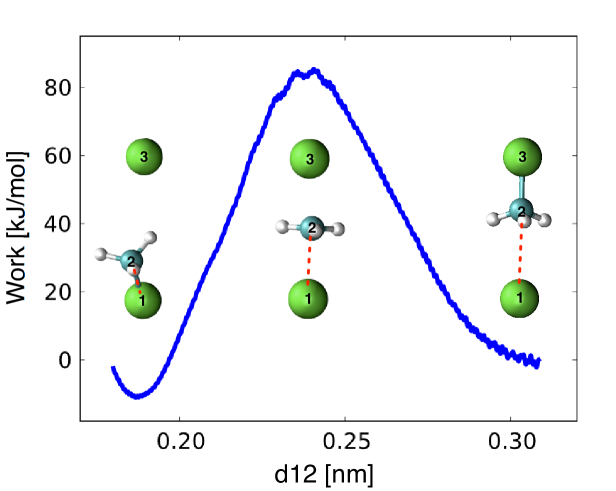
Figure 5: Worked performed during a steered MD simulation using as CV the distance (red dotted line) between a chlorine atom (atom 1) and the carbon atom of the methyl group (atom 2).

This input instructs PLUMED to calculate two distances but only one (the distance between atoms 1 and 2: 12 }) is use in the moving restraint. Initially, the equilibrium position for the harmonic potential is at

12 } equal to 0.31~nm,
thus ensuring that atoms 1 an

2 are not bonded. The center of the potential then moves at constant velocity to a value for 12 } of 0.18~nm uring the course of the 5 ps (5000 step) simulation. The potential is a harmonic spring with a force constant of 2$\times 10^{5}$ kJ mol^-1 nm^-2 so the motion of the center causes the system to move towards configurations in which the bond is formed. During the simulation PLUMED generates a file called

OLVAR }.  This file is
produced thanks to the {\verb PRINT } Action, which should always be used to output quantities calculated by the
various Actions in the input file.  The form of the {\verb PRINT } command in the input file above ensures that the
values of the distances {\verb d12 } and {\verb d23 } are output at every step  together with the equilibrium position for the
moving harmonic potential {\verb steer.d12_cntr } and the work {\verb steer.d12_work }, which is calculated using
equation~\ref{eqn:work}.  Figure~\ref{fig:steer-fig} shows a plot of the work performed by the potential as
it moves along the {\verb d12 } coordinate (from right to left).
As one would expect for a SN2 reaction of this kind a maximum for the work
appears when the methyl group is equidistant from the two chlorine atoms.
\subsection{Using functions of collective variables}
{\verb MATHEVAL } is one of the most powerful Actions in PLUMED 2. This Action can be used to construct
linear and non-linear functions of 

Vs with the libmatheval library [44]. The example input below shows how complex CVs can be calculated without making any modifications to PLUMED by using this Action in tandem with the simple CVs that are already present:

# just declare the RMSD^2 for five structures
t1: RMSD REFERENCE=c_1.pdb TYPE=OPTIMAL SQUARED
t2: RMSD REFERENCE=c_2.pdb TYPE=OPTIMAL SQUARED
t3: RMSD REFERENCE=c_3.pdb TYPE=OPTIMAL SQUARED
t4: RMSD REFERENCE=c_4.pdb TYPE=OPTIMAL SQUARED
t5: RMSD REFERENCE=c_5.pdb TYPE=OPTIMAL SQUARED
# calculate the sum of the exponential of the five RMSDs
MATHEVAL ...
 LABEL=dwn
 ARG=t1,t2,t3,t4,t5
 VAR=d1,d2,d3,d4,d5
 FUNC=(exp(-770*d1)+exp(-770*d2)+exp(-770*d3)+exp(-770*d4)+exp(-770*d5))
 PERIODIC=NO
... MATHEVAL
# now calculate the indexed sum
MATHEVAL ...
 LABEL=up
 ARG=t1,t2,t3,t4,t5
 VAR=d1,d2,d3,d4,d5
 FUNC=(exp(-770*d1)+2*exp(-770*d2)+3*exp(-770*d3)+4*exp(-770*d4)+5*exp(-770*d5))
 PERIODIC=NO
... MATHEVAL
# combine them into a progress function
MATHEVAL ...
 LABEL=s ARG=up,dwn VAR=u,d PERIODIC=NO
 FUNC=u/d
... MATHEVAL
# combine them into the distance from the path
MATHEVAL ...
 LABEL=z ARG=dwn VAR=d  PERIODIC=NO
 FUNC=-(1./770.)*log(d)
... MATHEVAL
# some printout
PRINT ARG=s,z STRIDE=100 FILE=colvar FMT=%
# do metadynamics with welltempered and adaptive hills
METAD ...
 HEIGHT=1.2 SIGMA=0.02 PACE=60
 ARG=s,z ADAPTIVE=GEOM BIASFACTOR=5 TEMP=300
... METAD

This input file uses

ATHEVAL } multiple times in order to generate non-linear combinations of the mean
square displacements from a number of different reference points.  The particular non-linear
combination we are creating are the path CVs of
Branduardi {\it et al.} \cite{bran+07jcp}.  These variables measure the progress $s$ along some curvilinear path in the
high-dimensional space:
%
\begin{equation}
s = \frac{\sum_{i=1}^5 i \exp(-\lambda 

_i(X)) ∑_i=1^5 exp(-λM_i(X)), and the distance $z$ from the path:

$$z=-\frac{1}{\lambda}\ln{\sum_{i=1}^{5}\exp(-\lambda M_{i}({\bf X}))},$$ (5)

where $M_{i}({\bf X})$ is the mean-square deviation, after optimal alignment, of a subset of the atoms from a reference structure denoted by the $i$ index. The parameter $\lambda$ is a smoothing parameter that can be set by examining the average distance between adjacent images. In the example input above, these $M_{i}$ values are calculated by the Actions labeled 1 }, {\verb 2 , 3 }, {\verb 4 and

5 }.
To be 

lear, path CVs are now quite widely used by the community and PLUMED 2 contains a simpler command (

ATHMSD }) that can be used to calculate these CVs.  Consequently, much
of the complexity in the input file above can be avoided by the casual user.  However, we believe this
example is still instructive as it demonstrates how complicated CVs can be generated in
the input file and how 

LUMED and the matheval library automatically look after the derivatives of these functions.

ATHEVAL } allows one to try new CV combinations without modifying the
interior of the code.
\begin{figure}
\centering
\includegraphics[height=9cm,angle=0]{Fig6}
\caption{The FES of alanine dipeptide as a function of the path CVs
discussed in the text.  This FES was calculated using a metadynamics simulation with
adaptive hills.}
\label{fig:diala-fes}
\end{figure}
The path defined in the above input is an optimized path for alanine dipeptide in vacuum that connects
the metastable states C7eq and Cax. We modeled this system using the CHAR

M27 forcefield [45, 46] as implemented in GROMACS 4.5.5 [7]. In order to see transitions between the $\rm C7_{eq}$ and $\rm C_{ax}$ states we performed a 3 ns well-tempered metadynamics simulation [47] using the geometry-adapted Gaussians scheme introduced by Branduardi et al. [48]. The free-energy surface (FES) shown in figure LABEL:fig:diala-fes was extracted by post-processing this simulation using a Torrie-Valleau correction [11, 48] and can be easily calculated using the post processing tools in PLUMED 2.

4.2 Using a function of a distribution of CVs

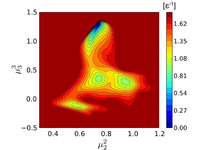
Figure 6: The FES for a seven-atom Lennard-Jones cluster as a function of the second and third moments of the distribution of coordination numbers. These CVs map the four known minima for this structure to different parts of the 2D plane. This FES was obtained by reweighting the result of a higher temperature MD simulation.

When devising CVs for clusters or bulk materials it is important to remember that the value of the CV should not change when the labels on atoms of the same type are exchanged. If a process such as nucleation is examined without considering this symmetry a large number of pathways connecting the liquid to the crystalline state will be found as the critical nuclei can be formed from any combination of the atoms in the system. In fact the number of pathways from the liquid to solid state is not analytically countable a priori. To examine these sorts of problems we therefore need global CVs that measure how a distribution of atomic/molecular order parameters changes. A common strategy is to calculate the values of some symmetry function (e.g. coordination numbers, Steinhardt parameters [49]) for each atom and to use the average of the distribution as a global CV [50]. It is known, however, that this often forces reactions to take place via a highly-concerted, unphysical mechanism. Furthermore, the mean will not necessarily separate all the structurally distinct configurations of a cluster or bulk solid. The average is not the only quantity one can calculate from a distribution of symmetry functions and there is strong evidence that calculating functions other than the average allows you to examine interesting phenomena [51, 52, 53]. Hence, within PLUMED 2 we provide tools to calculate the average of a distribution of symmetry functions, the moments of the distribution, the number of symmetry functions less than a certain value and so on all within the MultiColvar class. To demonstrate how this class can be used in practice we show here an example calculation on a well studied, two-dimensional, seven-atom Lennard-Jones cluster. This cluster is known to have four minima that appear at distinct points on the two dimensional plane described by the second ($\mu_{2}^{2}=\frac{1}{N}\sum_{i=1}^{N}\langle c_{i}-\overline{c}\rangle^{2}$) and third ($\mu_{3}^{3}=\frac{1}{N}\sum_{i=1}^{N}\langle c_{i}-\overline{c}\rangle^{3}$) moments of the distribution of coordination numbers [54, 29]. These quantities can be calculated by PLUMED 2 using the following command:

COORDINATIONNUMBER ...
 SPECIES=1-7
 SWITCH={RATIONAL R_0=1.5 NN=8 MM=16}
 MOMENTS=2-3
 LABEL=c1
... COORDINATIONNUMBER

Coordination numbers for each of the seven atoms are calculated using:

$$c_{i}(\mathbf{X})=\sum_{j\neq i}\frac{1-\left(\frac{d_{ij}(\mathbf{X})}{1.5}\right)^{8}}{1-\left(\frac{d_{ij}(\mathbf{X})}{1.5}\right)^{16}},$$ (6)

where $d_{ij}(\mathbf{X})$ is the distance between the $i$-th atom and the $j$-th atom. Then, once the coordination numbers have been calculated, the moments (and their derivatives) are calculated using the equations in the paragraph above and are stored so that they can be referenced in other Actions as 1.moment_2 } and {\verb 1.moment_3 .

To calculate the FES of seven-atom Lennard-Jones cluster as a function of the moments we ran an MD simulation at 0.2 $\frac{k_{B}T}{\epsilon}$. The final result of the calculation is shown in figure 6. The PLUMED 2 input for this calculation was as follows:

#
# instructs plumed to use LJ units for length and energy
#
UNITS NATURAL
#
# boundaries to prevent the system from subliming
#
COM ATOMS=1-7 LABEL=com
DISTANCE ATOMS=1,com LABEL=d1
UPPER_WALLS ARG=d1 AT=2.0 KAPPA=100.
DISTANCE ATOMS=2,com LABEL=d2
UPPER_WALLS ARG=d2 AT=2.0 KAPPA=100.
DISTANCE ATOMS=3,com LABEL=d3
UPPER_WALLS ARG=d3 AT=2.0 KAPPA=100.
DISTANCE ATOMS=4,com LABEL=d4
UPPER_WALLS ARG=d4 AT=2.0 KAPPA=100.
DISTANCE ATOMS=5,com LABEL=d5
UPPER_WALLS ARG=d5 AT=2.0 KAPPA=100.
DISTANCE ATOMS=6,com LABEL=d6
UPPER_WALLS ARG=d6 AT=2.0 KAPPA=100.
DISTANCE ATOMS=7,com LABEL=d7
UPPER_WALLS ARG=d7 AT=2.0 KAPPA=100.
#
# calculates moments of the coordination number distribution
#
COORDINATIONNUMBER ...
 SPECIES=1-7
 MOMENTS=2-3
 SWITCH={RATIONAL R_0=1.5 NN=8 MM=16}
 LABEL=c1
... COORDINATIONNUMBER
#
# calculate histograms from the moments
#
HISTOGRAM ...
 ARG=c1.moment_2,c1.moment_3 STRIDE=10
 REWEIGHT_TEMP=0.1 TEMP=0.2
 GRID_MIN=0.2,-0.5 GRID_MAX=1.2,1.7 GRID_BIN=200,440
 BANDWIDTH=0.01,0.01 KERNEL=triangular
 GRID_WSTRIDE=10000000 GRID_WFILE=histo
... HISTOGRAM

For this calculation we worked in Lennard-Jones units so lengths are in units of $\sigma$, energies are in units of $\epsilon$ and times are in units of $t^{*}=\sqrt{\frac{m\sigma^{2}}{\epsilon}}$. We introduced a set of restraints on the distances between the positions of the atoms in the cluster and the center of mass in order to prevent the cluster from subliming. We then ran $10^{7}$ steps of MD at a temperature of 0.2 $\frac{k_{B}T}{\epsilon}$ using the Lennard-Jones MD code (implemd }) that form part of PLUMED. The temperature in these simulations was kept fixed using a Langevin thermostat with a relaxation time of 1.0 $t^{*}$ and the timestep was 0.005 $t^{*}$. We extracted a FES at the lower temperature of 0.1 $\frac{k_{B}T}{\epsilon}$ by reweighting the probability distribution calculated at the higher temperature, $P(\mathbf{s})$, using $\exp(-(\frac{E(\mathbf{X})}{0.1}-\frac{E(\mathbf{X})}{0.2}))P(\mathbf{s})$. This analysis is done on the fly using PLUMED 2’s histogram utility, which performs kernel density estimation with triangular kernel functions. The FES shown in figure 6 is an average from 16 such runs. Each of these calculations was started from a different, equilibrated configuration. The standard deviations between the estimates of the free energies obtained from the individual runs were on the order of 0.05 $\epsilon$ over the whole FES.

5 Adding a new functionality to PLUMED 2

As shown in the examples above, the fact that the PLUMED 2 input file is written in a pseudo scripting language allows users to use a wide variety of CVs and methods. Even so, some users will eventually find themselves requiring something that is not implemented and that requires some coding. It is important to note at the outset that the object-oriented style of the code makes it straightforward to reuse features written by others. Developers should thus look carefully at the developer manual before starting programming so as to work out what functionality from the core can be reused. In particular, if they are interested in implementing a CV, a function of a CV, a biasing method or a method for analyzing the trajectory the developer manual contains step by step instructions as to how to go about performing these tasks.

The creation of a new piece of functionality usually involves the creation of a single new source code file, which, in the majority of cases, provides a definition for a new Action object. This file should eventually contain the definition of the class, the definitions for the methods in the class and the documentation for the new piece of functionality. Furthermore, any new Action object should inherit either directly or indirectly from the Action class. In this way new functionality can be added to PLUMED 2 through dynamic polymorphism and hence without modification of the PLUMED core. Methods in the new class with certain special name, e.g. alulate , will then be called at certain key points during the execution of each MD step and the new Action will be properly integrated into PLUMED. In addition, in classes that inherit from Action protected routines can be reused to output to the log file, to parse the input and to detect errors.

From discussions with the users we found that one reason for PLUMED 1’s success was the provision of a detailed manual. We thus felt it was important to ensure that good documentation was provided. Each Action in PLUMED 2 is described in the manual in a single page of HTML, which gives a brief description of what the Action calculates and what it can be used for, a description of the list of keywords for the Action and finally some examples of the Action’s use. These HTML pages are generated from descriptions in the individual source code files using Doxygen [55]. We felt that keeping the user documentation and source code together in this way was a good way of encouraging people to keep the manual consistent with the code. To write the documentation developers have to write a short paragraph of text and to provide some examples before the executable code in the source code file. In writing this text developers make use of Doxygen, which provides simple LaTeX-like commands that allow one to include equations and references. The list of available options or keywords for each Action and descriptions of the keywords is required to be placed inside the source as this information is also used to provide useful error messages. In addition, T. Giorgino has reused these keyword descriptions to provide templates for PLUMED GUI [16]. Finally, a side benefit of having keyword descriptions in the source is that a single piece of documentation for an often used keyword can be used in the descriptions of multiple Actions.

Developers modifying the code are strongly encouraged to use regtests. There is now a simple procedure for including a new test and all tests are run using a single script. Regularly running regtests as the code is developed allows one to ensure that new features are not breaking established functionalities in the code. Even developers working on code that is not being shared will benefit if they have regtests for new functionalities as they can use regtests to ensure that their new functionality continues to work when code is updated upstream.

Lastly, if users have exotic CVs or methods that they have used PLUMED to calculate we encourage them to share their experiences with the community. To help in this we have provided functionality for users and developers to share information through tutorials that can be added to the manual for the code.

6 Conclusion and outlook

New simulation techniques are oftentimes not rapidly exploited in the wider community because easy-to-use implementations of them are not readily available. PLUMED thus performs a vital service by disseminating new methods to the widest possible community of users in a form that can be added to many of the available MD engines.

With PLUMED 2 we have removed many of the limitations that were in PLUMED 1. It is now far easier to use new CVs as complex combinations of variables can be assembled directly from the input file. In addition, the performance of the code has been improved by parallelizing variables and by calculating them only when needed. One further, particularly-important improvement is that the interface between PLUMED and the MD engines has been simplified considerably. This will make maintenance easier and, given that PLUMED can now be compiled as a dynamic library, even give MD engine developers the option of providing their codes with the PLUMED interface in place already. This more flexible interface also makes it more straightforward to change the amount of information passed between the MD code and PLUMED. Hence, PLUMED could now easily be extended and used to implement features such as thermostats or force-fields. Furthermore, we believe that the internal flexibility of the new version will allow many more scientists to contribute new CVs, free-energy methods, and analysis tools. This will thus further foster the development of new techniques for MD.

7 Availability

PLUMED 2 can be downloaded from www.plumed-code.org. To best serve the community of PLUMED users and developers we have slightly changed the way the code is delivered. Now, as well as having stable releases of the code that can be downloaded from the website, we also provide read-only access to a git repository containing the development version of the code. For this reason we now have two mailgroups: the old plumed-users@googlegroups.com and plumed2-git@googlegroups.com. The second is designed for users and developers experimenting with the latest development version of the code which is available from www.plumed-code.org/git. Users who wish to distribute their own additional functionality for PLUMED can do so by either contacting the developers or by providing the additional code through their own websites.

8 Acknowledgments

The reworking of PLUMED 2 that has been described in this paper was made possible by a CeCAM grant and by a “Young SISSA Scientists’ Research Projects” scheme 2011-2012 that was promoted by the International School for Advanced Studies (SISSA), Trieste, Italy. Using funding from these sources we were able to organize a PLUMED tutorial, a developer meeting and a user meeting. These forums provided the opportunity to meet the various users and developers of the code and to find out the various problems with the original package. We would like to acknowledge all the people who attended these meetings for their feedback as well as the many users who have provided valued contributions to our mailing list. In particular, we would like to thank Paolo Elvati, Toni Giorgino, Alessandro Laio, Layla Martin-Samos, Michele Parrinello, Fabio Pietrucci and Paolo Raiteri for making time to discuss the code privately with the authors. In addition, GB and DB acknowledge the HPC-EUROPA2 project no. 228398, GB acknowledges MIUR grant FIRB (Futuro in Ricerca no. RBFR102PY5) and the European Research Council (Starting Grant S-RNA-S, no. 306662), and CC acknowledges support from a Marie Curie Intra European Fellowship.

References

- [1] Shaw, D. E. et al., Science 330 (2010) 341.
- [2] Frenkel, D. and Smit, B., Understanding molecular simulation: from algorithms to applications, Academic Press, 2 edition, 2002.
- [3] Tuckerman, M. E., Statistical Mechanics: Theory and Molecular Simulation, Oxford University Press, USA, 2010.
- [4] Smith, W., Leslie, M., and Forester, T. R., CCLRC, Daresbury Laboratory, Daresbury, England, Version 2.16.
- [5] Plimpton, S., J. Comput. Phys. 117 (1995) 1.
- [6] Phillips, J. C. et al., J. Comput. Chem. 26 (2005) 1781.
- [7] Hess, B., Kutzner, C., van der Spoel, D., and Lindahl, E., J. Chem. Theory Comput. 4 (2008) 435.
- [8] Giannozzi, P. et al., J. Phys.: Cond. Matter 21 (2009) 395502.
- [9] Case, D. et al., Amber 12, 2012, University of California, San Francisco.
- [10] Bonomi, M. et al., Comput. Phys. Comm. 180 (2009) 1961.
- [11] Torrie, G. M. and Valleau, J. P., J. Comput. Phys. 23 (1977) 187.
- [12] Laio, A. and Parrinello, M., Proc. Natl. Acad. Sci. U.S.A. 99 (2002) 12562.
- [13] Barducci, A., Bonomi, M., and Parrinello, M., Wires Comput. Mol. Sci. 1 (2011) 826.
- [14] Grubmüller, H., Heymann, B., and Tavan, P., Science 271 (1996) 997.
- [15] Fiorin, G., Klein, M. L., and Henin, J., Mol. Phys. (2013).
- [16] Giorgino, T., Comput. Phys. Comm. (2013), submitted.
- [17] Biarnes, X., Pietrucci, F., Marinelli, F., and Laio, A., Comput. Phys. Comm. 183 (2012) 203.
- [18] Ceriotti, M., Tribello, G. A., and Parrinello, M., Proc. Natl. Acad. Sci. U.S.A. 108 (2011) 13023–.
- [19] Rohrdanz, M. A., Zheng, W., and Clementi, C., Ann. Rev. Phys. Chem. 64 (2013) 295.
- [20] Humphrey, W., Dalke, A., and Schulten, K., J. Molec. Graphics 14 (1996) 33.
- [21] Roe, D. R. and Cheatham, T. E., J. Chem. Theory Comput. 9 (2013) 3084.
- [22] Seeber, M., Cecchini, M., Rao, F., Settanni, G., and Caflisch, A., Bioinformatics 23 (2007) 2625.
- [23] Seeber, M. et al., J. Comput. Chem. 6 (2011) 1183.
- [24] Glykos, N. M., J. Comput. Chem. 27 (2006) 1765.
- [25] Bowers, K. J. et al., Scalable algorithms for molecular dynamics simulations on commodity clusters, in Proceedings of the 2006 ACM/IEEE conference on Supercomputing, SC ’06, New York, NY, USA, 2006, ACM.
- [26] Marsili, S., Signorini, G. F., Chelli, R., Marchi, M., and Procacci, P., J. Comput. Chem. 31 (2010) 1106.
- [27] Eastman, P. et al., J. Chem. Theory Comput. 9 (2013) 461.
- [28] Maragakis, P., van der Vaart, A., and Karplus, M., J. Phys. Chem. B 113 (2009) 4664.
- [29] Tribello, G. A., Ceriotti, M., and Parrinello, M., Proc. Natl. Acad. Sci. U.S.A. 107 (2010) 17509.
- [30] Piana, S. and Laio, A., J. Phys. Chem. B 111 (2007) 4553.
- [31] Kearsley, S. K., Acta Cryst. A 45 (1989) 208.
- [32] Branduardi, D., Gervasio, F. L., and Parrinello, M., J. Chem. Phys. 126 (2007) 054103.
- [33] Pietrucci, F. and Laio, A., J. Chem. Theory Comput. 5 (2009) 2197.
- [34] Spiwok, V. and Králová, B., J. Chem. Phys. 135 (2011) 224504.
- [35] Vymětal, J. and Vondrášek, J., J. Phys. Chem. A 115 (2011) 11455.
- [36] Bonomi, M. and Parrinello, M., Phys. Rev. Lett. 104 (2010) 190601.
- [37] Do, T. N., Carloni, P., Varani, G., and Bussi, G., J. Chem. Theory Comput. 9 (2013) 1720.
- [38] Robustelli, P., Kohlhoff, K., Cavalli, A., and Vendruscolo, M., Structure 18 (2010) 923.
- [39] Camilloni, C., Robustelli, P., De Simone, A., Cavalli, A., and Vendruscolo, M., J. Am. Chem. Soc. 134 (2012) 3968.
- [40] Bussi, G., Gervasio, F. L., Laio, A., and Parrinello, M., J. Am. Chem. Soc. 128 (2006) 13435.
- [41] Raiteri, P., Laio, A., Gervasio, F. L., Micheletti, C., and Parrinello, M., J. Phys. Chem. B 110 (2006) 3533.
- [42] http://www.mpi-forum.org.
- [43] Jarzynski, C., Phys. Rev. Lett. 78 (1997) 2690.
- [44] Samardzic, A., libmatheval, http://www.gnu.org/software/libmatheval/.
- [45] MacKerell, A. D. et al., J. Phys. Chem. B 102 (1998) 3586.
- [46] MacKerell Jr., A. D., Feig, M., and Brooks III, C. L., J. Comput. Chem. 25 (2004) 1400.
- [47] Barducci, A., Bussi, G., and Parrinello, M., Phys. Rev. Lett. 100 (2008) 020603.
- [48] Branduardi, D., Bussi, G., and Parrinello, M., J. Chem. Theory Comput. 8 (2012) 2247.
- [49] Steinhardt, P. J., Nelson, D. R., and Ronchetti, M., Phys. Rev. B 28 (1983) 784.
- [50] Quigley, D. and Rodger, P., J. Chem. Phys. 128 (2008) 154518.
- [51] Oganov, A. R. and Valle, M., J. Chem. Phys. 130 (2009) 104504.
- [52] Tribello, G. A., Cuny, J., Eshet, H., and Parrinello, M., J. Chem. Phys. 135 (2011) 114109.
- [53] Ceriotti, M., Tribello, G. A., and Parrinello, M., J. Chem. Theory Comput. 9 (2013) 1521.
- [54] Wales, D. J., Mol. Phys. 100 (2002) 3285.
- [55] van Heesch, D., doxygen, http://www.stack.nl/dimitri/doxygen.