Exact and Stable Covariance Estimation
from Quadratic Sampling via Convex Programming

Abstract

Statistical inference and information processing of high-dimensional data often require efficient and accurate estimation of their second-order statistics. With rapidly changing data, limited processing power and storage at the acquisition devices, it is desirable to extract the covariance structure from a single pass over the data and a small number of stored measurements. In this paper, we explore a quadratic (or rank-one) measurement model which imposes minimal memory requirements and low computational complexity during the sampling process, and is shown to be optimal in preserving various low-dimensional covariance structures. Specifically, four popular structural assumptions of covariance matrices, namely low rank, Toeplitz low rank, sparsity, jointly rank-one and sparse structure, are investigated, while recovery is achieved via convex relaxation paradigms for the respective structure.

The proposed quadratic sampling framework has a variety of potential applications including streaming data processing, high-frequency wireless communication, phase space tomography and phase retrieval in optics, and non-coherent subspace detection. Our method admits universally accurate covariance estimation in the absence of noise, as soon as the number of measurements exceeds the information theoretic limits. We also demonstrate the robustness of this approach against noise and imperfect structural assumptions. Our analysis is established upon a novel notion called the mixed-norm restricted isometry property (RIP-$\ell_{2}/\ell_{1}$), as well as the conventional RIP-$\ell_{2}/\ell_{2}$ for near-isotropic and bounded measurements. In addition, our results improve upon the best-known phase retrieval (including both dense and sparse signals) guarantees using PhaseLift with a significantly simpler approach.

I Introduction

Accurate estimation of second-order statistics of stochastic processes and data streams is of ever-growing importance to various applications that exhibit high dimensionality. Covariance estimation is the cornerstone of modern statistical analysis and information processing, as the covariance matrix constitutes the sufficient statistics to many signal processing tasks, and is particularly crucial for extracting reduced-dimension representation of the objects of interest. For signals and data streams of high dimensionality, there might be limited memory and computation power available at the data acquisition devices to process the rapidly changing input, which requires the covariance estimation task to be performed with a single pass over the data stream, minimal storage, and low computational complexity. This is not possible unless appropriate structural assumptions are incorporated into the high-dimensional problems. Fortunately, a broad class of high-dimensional signals indeed possesses low-dimensional structures, and the intrinsic dimension of the covariance matrix is often far smaller than the ambient dimension. For different types of data, the covariance matrix may exhibit different structures; four of the most widely considered structures are listed below.

• Low Rank: The covariance matrix is (approximately) low-rank, which occurs when a small number of components accounts for most of the variability in the data. Low-rank covariance matrices arise in applications including traffic data monitoring, array signal processing, collaborative filtering, and metric learning.

• Stationarity and Low Rank: The covariance matrix is simultaneously low-rank and Toeplitz, which arises when the random process is generated by a few spectral spikes. Recovery of the stationary covariance matrix, often equivalent to spectral estimation, is crucial in many tasks in wireless communications (e.g. detecting spectral holes in cognitive radio networks), and array signal processing (e.g. direction-of-arrival analysis [3]).

• Sparsity: The covariance matrix can be approximated in a sparse form [4]. This arises when a large number of variables have small pairwise correlation, or when several variables are mutually exclusive. Sparse covariance matrices arise in finance, biology and spectrum estimation.

• Joint Sparsity and Rank-One: The covariance matrix can be approximated by a jointly sparse and rank-one matrix. This has received much attention in recent development of sparse PCA, and is closely related to sparse signal recovery from magnitude measurements (called sparse phase retrieval).

In this paper, we wish to reconstruct an unknown covariance matrix ${\boldsymbol{\Sigma}}\in\mathbb{R}^{n\times n}$ with the above structure from a small number of rank-one measurements. In particular, we explore sampling methods of the form

$$y_{i} ={\boldsymbol{a}}_{i}^{\top}{\boldsymbol{\Sigma}}{\boldsymbol{a}}_{i}+\eta_{i},\quad i=1,\ldots,m,$$ (1)

where $\boldsymbol{y}:=\left\{y_{i}\right\}_{i=1}^{m}$ denotes the measurements, ${\boldsymbol{a}}_{i}\in\mathbb{R}^{n}$ represents the sensing vector, ${\boldsymbol{\eta}}:=\left\{\eta_{i}\right\}_{i=1}^{m}$ stands for the noise term, and $m$ is the number of measurements. The noise-free measurements ${\boldsymbol{a}}_{i}^{\top}{\boldsymbol{\Sigma}}{\boldsymbol{a}}_{i}$’s are henceforth referred to as quadratic measurements (or rank-one measurements). In practice, the number of measurements one can obtain is constrained by the storage requirement in data acquisition, which could be much smaller than the ambient dimension of ${\boldsymbol{\Sigma}}$. This sampling scheme finds applications in a wide spectrum of practical scenarios, admits optimal covariance estimation with tractable algorithms, and brings in computational and storage advantages in comparison with other types of measurements, as detailed in the rest of the paper.

I-A Motivation

The quadratic measurements in the form of (1) are motivated by several application scenarios listed below, which illustrate the practicability and benefits of the proposed quadratic measurement scheme.

I-A1 Covariance Sketching for Data Streams

A high-dimensional data stream model represents real-time data that arrives sequentially at a high rate, where each data instance is itself high-dimensional. In many resource-constrained applications, the available memory and processing power at the data acquisition devices are severely limited compared with the volume and rate of the data [5]. Therefore it is desirable to extract the covariance matrix of the data instances from inputs on the fly without storing the whole stream. Interestingly, the quadratic measurement strategy can be leveraged as an effective data stream processing method to extract the covariance information from real-time data, with limited memory and low computational complexity.

Specifically, consider an input stream $\{\boldsymbol{x}_{t}\}_{t=1}^{\infty}$ that arrives sequentially, where each $\boldsymbol{x}_{t}\in\mathbb{R}^{n}$ is a high-dimensional data instance generated at time $t$. The goal is to estimate the covariance matrix $\boldsymbol{\Sigma}=\mathbb{E}[\boldsymbol{x}_{t}\boldsymbol{x}_{t}^{\top}]\in\mathbb{R}^{n\times n}$. The prohibitively high rate at which data is generated forces covariance extraction to function with as small a memory as possible. The scenario we consider is quite general, and we only impose that the covariance of a random substream of the original data stream converges to the true covariance ${\boldsymbol{\Sigma}}$. No prior information on the correlation statistics across consecutive instances is assumed to be known a priori (e.g. they are not necessarily independently drawn), and hence it is not feasible to exploit these statistics to enable lower sample complexity.

We propose to pool the data stream $\{\boldsymbol{x}_{t}\}_{t=1}^{\infty}$ into a small set of measurements in an easy-to-adapt fashion with a collection of sketching vectors $\{{\boldsymbol{a}}_{i}\}_{i=1}^{m}$. Our covariance sketching method, termed quadratic sketching, is outlined as follows:

1. At each time $t$, we randomly choose a sketching vector indexed by $\ell_{t}\in\{1,\ldots,m\}$, and obtain a single nonnegative quadratic sketch $(\boldsymbol{a}_{\ell_{t}}^{\top}\boldsymbol{x}_{t})^{2}$.

2. All sketches employing the same sketching vector ${\boldsymbol{a}}_{i}$ are aggregated and normalized, which converge rapidly to a measurement

   $$y_{i} =\mathbb{E}\left[(\boldsymbol{a}_{i}^{\top}\boldsymbol{x}_{t})^{2}\right]+{\boldsymbol{\eta}}_{i}={\boldsymbol{a}}_{i}^{\top}\mathbb{E}\left[{\boldsymbol{x}}_{t}{\boldsymbol{x}}_{t}^{\top}\right]{\boldsymbol{a}}_{i}+{\boldsymbol{\eta}}_{i}$$

   $$=\boldsymbol{a}_{i}^{\top}\boldsymbol{\Sigma}\boldsymbol{a}_{i}+{\boldsymbol{\eta}}_{i},\quad\quad\quad i=1,\ldots,m,$$ (2)

   where ${\boldsymbol{\eta}}:=\left\{\eta_{i}\right\}_{i=1}^{m}$ denotes the error term.

There are several benefits of this covariance sketching method. First, the storage complexity $m$, as will be shown, can be much smaller than the ambient dimension of ${\boldsymbol{\Sigma}}$. The computational cost for sketching each instance is linear with respect to the dimension of the instance in the data stream. Unlike the uncompressed sketching methods where each instance one measures usually affects many stored measurements, our scheme allows each aggregate quadratic sketch to be composed by completely different instances, which allows sketching to be performed in a distributed and asynchronous manner. This arises since each randomized sketch is a compressive snapshot of the second-order statistics, while each uncompressed measurement itself is unable to capture the correlation information. As we will demonstrate later, this sketching scheme allows optimal covariance estimation with information theoretically minimal memory complexity at the data acquisition stage. One motivating application for this covariance sketching method is covariance estimation of ultra-wideband random processes, as is further elaborated in Section I-A2.

I-A2 Noncoherent Energy Measurements in Communications and Signal Processing

When communication takes place in the high-frequency regime, empirical energy measurements are often more accurate and cheaper to obtain than phase measurements. For instance, energy measurements will be more reliable when communication systems are operating with extremely high carrier frequencies (e.g. 60GHz communication systems [6]).

• Spectrum Estimation of Stochastic Processes from Energy Measurements: Many wireless communication systems operating in stochastic environments rely on reliable estimation of the spectral characteristics of random processes [7], such as recovering the power spectrum of the ultra-wideband random process characterizing the spectrum occupancy in cognitive radio [8, 9]. Moreover, optimal signal transmissions are often based on the Karhunen–Loeve decomposition of a random process, which requires accurate covariance information [10]. If one employs a sensing vector $\boldsymbol{a}_{i}$, which is implementable using random demodulators [11], and observes the average energy measurements over $N$ instances $\left\{\boldsymbol{x}_{t}\right\}_{1\leq t\leq N}$, then the energy measurements read

  $$y_{i}=\frac{1}{N}\sum_{t=1}^{N}\left|{\boldsymbol{a}}_{i}^{\top}{\boldsymbol{x}}_{t}\right|^{2}={\boldsymbol{a}}_{i}^{\top}{\boldsymbol{\Sigma}}_{N}{\boldsymbol{a}}_{i},\quad i=1,\ldots,m$$ (3)

  where ${\boldsymbol{\Sigma}}_{N}:=\frac{1}{N}\sum_{t=1}^{N}{\boldsymbol{x}}_{t}{\boldsymbol{x}}_{t}^{\top}$ denotes the sample covariance matrix, leading to the quadratic-form observations.

• Noncoherent Subspace Detection from Energy Measurements: Matched subspace detection [12] spans many applications in wireless communication, radar, and pattern recognition when the transmitted signal is encoded by the subspaces. The problem can also be cast as recovering the principal subspace of a dataset $\{{\boldsymbol{x}}_{t}\}_{t=1}^{N}$, with an energy detector obtaining $m$ measurements in the form of (3). Thus, the noncoherent subspace detection is subsumed by the formulation (1).

I-A3 Phaseless Measurements in Physics

Optical imaging devices are incapable of acquiring phase measurements due to ultra-high frequencies associated with light. In many applications, measurements taking the form of (1) arise naturally.

• Compressive Phase Space Tomography: Phase Space Tomography [13] is an appealing method to measure the correlation function of a wave field in physics. However, tomography becomes challenging when the dimensionality of the correlation matrix becomes large. Recently, it was proposed experimentally in [14] to recover an approximately low-rank correlation matrix, which often holds in physics, by only taking a small number of measurements in the form of (1).

• Phase Retrieval: Due to the physical constraints, one can only measure amplitudes of the Fourier coefficients of an optical object. This gives rise to the problem of recovering a signal $\boldsymbol{x}\in\mathbb{R}^{n}$ from magnitude measurements, which is often referred to as phase retrieval. Several convex (e.g. [15, 16, 17]) and nonconvex algorithms (e.g. [18, 19, 20, 21]) have been proposed that enable exact phase retrieval (i.e. recovers $\boldsymbol{x}\cdot\boldsymbol{x}^{\top}$) from random magnitude measurements. If we set ${\boldsymbol{\Sigma}}:=\boldsymbol{x}\boldsymbol{x}^{\top}$, then our problem formulation (1) subsumes phase retrieval as a special case in the low-rank setting.

Apart from the preceding applications, we are aware that this rank-one measurement model naturally arises in the mixture of linear regression problem [22]. All in all, all of these applications require structured matrix recovery from a small number of rank-one measurements (1). The aim of this paper to develop tractable recovery algorithms that enjoy near-optimal performance guarantees.

I-B Contributions

Our main contributions are three fold. First, we have developed convex optimization algorithms for covariance estimation from a set of quadratic measurements as given in (1) for a variety of structural assumptions including low-rank, Toeplitz low-rank, sparse, and sparse rank-one covariance matrices. The proposed algorithms exploit the presumed low-dimensional structures using convex relaxation tailored for respective structures. For a large class of sub-Gaussian sensing vectors, we derive theoretical performance guarantees (Theorems 1 – 4) from the following aspects:

1. Exact and universal recovery: once the sensing vectors are selected, then with high probability, all covariance matrices satisfying the presumed structure can be recovered;

2. Stable recovery: the proposed algorithms allow reconstruction of the true covariance matrix to within high accuracy even under imperfect structural assumptions; additionally, if the measurements are corrupted by noise, possibly adversarial, the estimate deviates from the true covariance matrix by at most a constant multiple of the noise level;

3. Near-minimal measurements: the proposed algorithms succeed as soon as the number of measurements is slightly above the information theoretic limits for most of the respective structure. For the special case of (sparse) rank-one matrices, our result recovers and strengthens the best-known reconstruction guarantees of (sparse) phase retrieval using PhaseLift [15, 23, 24] with a much simpler proof technique.

Secondly, to obtain some of the above theoretical guarantees (Theorems 1, 3, and 4), we have introduced a novel mixed-norm restricted isometry property, denoted by RIP-$\ell_{2}/\ell_{1}$. An operator is said to satisfy the RIP-$\ell_{2}/\ell_{1}$ if the strength of the signal class of interest before and after measurements are preserved when measured in the $\ell_{2}$ norm and in the $\ell_{1}$ norm, respectively. While the conventional RIP-$\ell_{2}/\ell_{2}$ does not hold for the quadratic sensing model for general low-rank structures as pointed out by [15], we have established that the sensing mechanism does satisfy the RIP-$\ell_{2}/\ell_{1}$ after a “debiasing” modification, under general low-rank, sparse, and simultaneously sparse and rank-one structural assumptions. This seemingly subtle change enables a significantly simpler analytical approach without resorting to complicated dual construction as in [15, 23, 24].

On the other hand, we demonstrate, via the entropy method [25], that linear combinations of the quadratic measurements satisfy RIP-$\ell_{2}/\ell_{2}$ when restricted to Toeplitz low-rank covariance matrices. This leads to near-optimal recovery guarantees for Toeplitz low-rank covariance matrices (Theorem 2). Along the way, we have also established a RIP-$\ell_{2}/\ell_{2}$ for bounded and near-isometric operators (Theorem 5), which strengthens previous work [26, 27] by offering universal and stable recovery guarantees for a broader class of operators including Fourier-type measurements.

Last but not least, our measurement schemes and algorithms may be of independent interest to high-dimensional data processing. The measurements in (1) are rank-one measurements with respect to the covariance matrix, which are much easier to implement and bear a smaller computational cost than full-rank measurement matrices with i.i.d. entries. Moreover, the performance guarantees of the measurement scheme (1) is universal, which does not require any additional incoherence conditions on the covariance matrix as required in the standard matrix completion framework [28, 26, 29].

I-C Related Work

In most existing work, the covariance matrix is estimated from a collection of full data samples, and fundamental guarantees have been derived on how many samples are sufficient to approximate the ground truth [30, 4]. In contrast, this paper is motivated by the success of Compressed Sensing (CS) [31, 32], which asserts that compression can be achieved at the same time as sensing without losing information. Efficient algorithms have been developed to estimate a deterministic signal from a much smaller number of linear measurements that is proportional to the complexity of the parsimonious signal model. As we will show in this paper, covariance estimation from compressive measurements can be highly robust.

When the covariance matrix is assumed to be approximately sparse, recent work [33, 8] explored reconstruction of second-order statistics of a cyclostationary signal from random linear measurements, by $\ell_{1}$-minimization without performance guarantees. Other spectral prior information has been considered as well in [34] for stationary processes. These problem setups are quite different from (1) in the current work. Another work by Dasarathy et al. [35] proposed estimating an approximately sparse covariance matrix from measurements of the form $\boldsymbol{Y}=\boldsymbol{A}{\boldsymbol{\Sigma}}\boldsymbol{A}^{\top}$, where $\boldsymbol{A}\in\mathbb{R}^{m\times n}$ denotes the sketching matrix constructed from expander graphs. Nevertheless, this scheme cannot accommodate low-rank covariance matrix estimation.

Our covariance estimation method is inspired by recent developments in phase retrieval [15, 23, 36, 37, 17, 20], which is tantamount to recovering rank-one covariance matrices from quadratic measurements. In particular, our recovery algorithm coincides with PhaseLift [15, 23] when applied to low-rank matrices. In [23], it is shown that PhaseLift succeeds at reconstructing a signal of dimensionality $n$ from $\Theta(n)$ phaseless Gaussian measurements, and stable recovery has also been established in the presence of noise. When specializing our result to this case, we have shown that the same type of theoretical guarantee holds for a much larger class of sub-Gaussian measurements, with a different proof technique that yields a much simpler proof. Moreover, when the signal is further assumed to be $k$-sparse, the pioneering work [24] showed that $O(k^{2}\log n)$ Gaussian measurements suffice; this result is extended to accommodate sub-Gaussian measurements and approximately sparse signals by our framework with a much simpler proof. More details can be found in Section II-D.

We also put the proposed covariance sketching scheme in Section I-A1 into perspective. In a streaming setting, online principal component analysis (PCA) has been an active area of research for decades [38] using full data samples, where non-asymptotic convergence guarantees have only been recently developed [39]. Inspired by CS, subspace tracking from partial observations of a data stream [40, 41], which can be regarded as a variant of incremental PCA [42] in the presence of missing values, is also closely related. However, existing subspace tracking algorithms mainly aim to recover the data stream, which is not necessary if one only cares to extract the second-order statistics.

Finally, after we posted our work on Arxiv, Cai and Zhang made available their manuscript [43], an independent work that studies low-rank matrix recovery under rank-one measurements via the notion of restricted uniform boundedness. In comparison, our results accommodate a larger class of covariance structures including Toeplitz low-rank, sparse, and jointly low-rank and sparse matrices.

I-D Organization

The rest of this paper is organized as follows. We first present the convex optimization based algorithms in Section II, and establish their theoretical guarantees. The analysis framework is based upon a novel mixed-norm restricted isometry property as well as conventional RIP for near-isotropic and bounded measurements, as elaborated in Sections III and IV. The proof of main theorems is deferred to the appendices. Numerical examples are provided in Sections V. Finally, Section VI concludes the paper with a summary of our findings and a discussion of future directions.

I-E Notations

Before proceeding, we provide a brief summary of useful notations that will be used throughout this paper. A variety of matrix norms will be discussed; in particular, we denote by $\left\|\boldsymbol{X}\right\|$, $\left\|\boldsymbol{X}\right\|_{\text{F}}$, and $\left\|\boldsymbol{X}\right\|_{*}$ the spectral norm, the Frobenius norm, and the nuclear norm (i.e. sum of all singular values) of $\boldsymbol{X}$, respectively. When ${\boldsymbol{X}}$ is a positive semidefinite (PSD) matrix, the nuclear norm coincides with the trace $\|{\boldsymbol{X}}\|_{*}=\operatorname{Tr}({\boldsymbol{X}})$. We use $\|{\boldsymbol{X}}\|_{1}$ and $\|{\boldsymbol{X}}\|_{0}$ to denote the $\ell_{1}$ norm and support size of the vectorized ${\boldsymbol{X}}$, respectively. The Euclidean inner product between $\boldsymbol{X}$ and $\boldsymbol{Y}$ is defined as $\left\langle\boldsymbol{X},\boldsymbol{Y}\right\rangle=\operatorname{Tr}(\boldsymbol{X}^{\top}\boldsymbol{Y})$. We will abuse the notation and let $\boldsymbol{\Sigma}_{r}$ and $\boldsymbol{\Sigma}_{k}$ stand for the best rank-$r$ approximation and the best $k$-term approximation of $\boldsymbol{\Sigma}$ respectively, i.e.

$$\boldsymbol{\Sigma}_{r}=\operatorname{argmin}_{\boldsymbol{M}:\text{rank}\left(\boldsymbol{M}\right)=r}\left\|\boldsymbol{\Sigma}-\boldsymbol{M}\right\|_{\mathrm{F}},$$

and

$$\boldsymbol{\Sigma}_{k}=\operatorname{argmin}_{\boldsymbol{M}:\left\|\boldsymbol{M}\right\|_{0}=k}\left\|\boldsymbol{\Sigma}-\boldsymbol{M}\right\|_{\mathrm{F}},$$

whenever clear from context. Besides, we denote by $\mathcal{T}$ the orthogonal projection operator onto Toeplitz matrices, and $\mathcal{T}^{\perp}$ its orthogonal complement. Some useful notations are summarized in Table I.

TABLE I: Summary of Notation and Parameters

${\boldsymbol{\Sigma}}$, ${\boldsymbol{\Sigma}}_{r}$, ${\boldsymbol{\Sigma}}_{\mathrm{c}}$	true covariance matrix, best rank-$r$ approximation of ${\boldsymbol{\Sigma}}$, and ${\boldsymbol{\Sigma}}_{\mathrm{c}}:={\boldsymbol{\Sigma}}-{\boldsymbol{\Sigma}}_{r}$
${\boldsymbol{\Sigma}}$, ${\boldsymbol{\Sigma}}_{\Omega_{0}}$, ${\boldsymbol{\Sigma}}_{\Omega_{0}^{\text{c}}}$	true covariance matrix, best $k$-sparse approximation of ${\boldsymbol{\Sigma}}$, and ${\boldsymbol{\Sigma}}_{\Omega_{0}^{\text{c}}}:={\boldsymbol{\Sigma}}-{\boldsymbol{\Sigma}}_{\Omega_{0}}$
$\mathcal{T}$, $\mathcal{T}^{\perp}$	orthogonal projection operator onto Toeplitz matrices, and its orthogonal complement.
${\boldsymbol{\eta}},\boldsymbol{y}\in\mathbb{R}^{m}$ ,	noise, quadratic measurements $\left\{\boldsymbol{a}_{i}^{\top}{\boldsymbol{\Sigma}}\boldsymbol{a}_{i}+\eta_{i}\right\}_{1\leq i\leq m}$
$\boldsymbol{a}_{i}\in\mathbb{R}^{n}$, $\boldsymbol{A}_{i}\in\mathbb{R}^{n\times n}$	$i$th sensing vector, $i$th sensing matrix $\boldsymbol{A}_{i}:=\boldsymbol{a}_{i}\cdot\boldsymbol{a}_{i}^{\top}$
$\boldsymbol{B}_{i}\in\mathbb{R}^{n\times n}$	auxiliary sensing matrix
$\mathcal{A}_{i}$,$\mathcal{A}$	linear transformation $\boldsymbol{X}\mapsto\boldsymbol{a}_{i}^{\top}\boldsymbol{X}\boldsymbol{a}_{i}$ , linear mapping $\boldsymbol{X}\mapsto\left\{\boldsymbol{a}_{i}^{\top}\boldsymbol{X}\boldsymbol{a}_{i}\right\}_{1\leq i\leq m}$
$\mathcal{B}_{i}$,$\mathcal{B}$	linear transformation $\boldsymbol{X}\mapsto\left\langle\boldsymbol{B}_{i},\boldsymbol{X}\right\rangle$ , linear mapping $\boldsymbol{X}\mapsto\left\{\mathcal{B}_{i}\left(\boldsymbol{X}\right)\right\}_{1\leq i\leq m}$

II Convex Relaxation and Its Performance Guarantees

In general, recovering the covariance matrix ${\boldsymbol{\Sigma}}\in\mathbb{R}^{n\times n}$ from $m<n(n+1)/2$ measurements is ill-posed, unless the sampling mechanism can effectively exploit the low-dimensional covariance structure. Random sampling often preserves the information structure from minimal observations, and allows robust recovery from noisy measurements.

In this paper, we restrict our attention to the following random sampling model. We assume that the sensing vectors are composed of i.i.d. sub-Gaussian entries. In particular, we assume ${\boldsymbol{a}}_{i}$’s ($1\leq i\leq m$) are i.i.d. copies of $\boldsymbol{z}=\left[z_{1},\cdots,z_{n}\right]^{\top}$, where each $z_{i}$ is i.i.d. drawn from a distribution with the following properties

$$\mathbb{E}[z_{i}]=0,\quad\mathbb{E}[z_{i}^{2}]=1,\quad\mbox{and}\quad\mu_{4}:=\mathbb{E}\left[z_{i}^{4}\right]>1.$$ (4)

We assume that the error term ${\boldsymbol{\eta}}:=[\eta_{1},\cdots,\eta_{m}]^{\top}$ is bounded in either $\ell_{1}$ norm or $\ell_{2}$ norm as specified later in the theoretical guarantees. For notational simplicity, let $\boldsymbol{A}_{i}:=\boldsymbol{a}_{i}\boldsymbol{a}_{i}^{\top}$ represent the equivalent sensing matrix, and hence the measurements $\boldsymbol{y}:=\left[y_{1},\cdots,y_{m}\right]^{\top}$ obeys $y_{i}:=\left\langle\boldsymbol{A}_{i},{\boldsymbol{\Sigma}}\right\rangle+\eta_{i}$. We also define the linear operator ${\mathcal{A}}(\boldsymbol{M}):\mathbb{R}^{n\times n}\mapsto\mathbb{R}^{m}$ that maps a matrix $\boldsymbol{M}\in\mathbb{R}^{n\times n}$ to $\{\langle\boldsymbol{M},{\boldsymbol{A}}_{i}\rangle\}_{i=1}^{m}$. These notations allow us to express the measurements as

$${\boldsymbol{y}}=\mathcal{A}({\boldsymbol{\Sigma}})+{\boldsymbol{\eta}}.$$ (5)

II-A Recovery of Low-Rank Covariance Matrices

Suppose that $\boldsymbol{\Sigma}$ is approximately low-rank, a natural heuristic is to perform rank minimization to encourage the low-rank structure

$$\hat{{\boldsymbol{\Sigma}}}=\operatorname{argmin}_{\boldsymbol{M}}\mbox{rank}(\boldsymbol{M})\quad\mbox{subject to} \quad\boldsymbol{M}\succeq 0,$$ (6)

$$\quad\|{\boldsymbol{y}}-\mathcal{A}(\boldsymbol{M})\|_{1}\leq\epsilon_{1},$$

where $\epsilon_{1}$ is an upper bound on $\left\|\boldsymbol{\eta}\right\|_{1}$ and assumed known a priori. However, the rank minimization problem is in general NP-hard. Therefore, we replace it with trace minimization over all matrices compatible with the measurements

$$\hat{{\boldsymbol{\Sigma}}}=\operatorname{argmin}_{\boldsymbol{M}}\operatorname{Tr}(\boldsymbol{M})\quad\mbox{subject to} \quad\boldsymbol{M}\succeq 0,$$ (7)

$$\quad\|{\boldsymbol{y}}-\mathcal{A}(\boldsymbol{M})\|_{1}\leq\epsilon_{1}.$$

Since ${\boldsymbol{\Sigma}}$ is PSD, the trace norm forms a convex surrogate for the rank function, which has proved successful in matrix completion and phase retrieval problems [28, 44, 15]. It turns out that this convex relaxation approach (7) admits stable and faithful estimates even when ${\boldsymbol{\Sigma}}$ is approximately low rank and/or when the measurements are corrupted by bounded noise. This is formally stated in the following theorem.

Theorem 1.

Consider the sub-Gaussian sampling model in (4) and assume that $\left\|\boldsymbol{\eta}\right\|_{1}\leq\epsilon_{1}$. Then with probability exceeding $1-C_{0}\exp(-c_{0}m)$, the solution $\hat{{\boldsymbol{\Sigma}}}$ to (7) satisfies

$$\|\hat{{\boldsymbol{\Sigma}}}-{\boldsymbol{\Sigma}}\|_{\mathrm{F}}\leq C_{1}\frac{\left\|{\boldsymbol{\Sigma}}-{\boldsymbol{\Sigma}}_{r}\right\|_{*}}{\sqrt{r}}+C_{2}\frac{\epsilon_{1}}{m}$$ (8)

simultaneously for all ${\boldsymbol{\Sigma}}\in\mathbb{R}^{n\times n}$, provided that $m>c_{1}nr$. Here, ${\boldsymbol{\Sigma}}_{r}$ represents the best rank-$r$ approximation of ${\boldsymbol{\Sigma}}$, and $c_{0}$, $c_{1}$, $C_{0}$, $C_{1}$ and $C_{2}$ are some positive numerical constants.

The main implications of Theorem 1 and its associated performance bound (8) are listed as follows.

1. Exact Recovery from Noiseless Measurements. Consider the case where $\text{rank}\left({\boldsymbol{\Sigma}}\right)=r$. In the absence of noise, one can see from (8) that the trace minimization program (7) (with $\epsilon_{1}=0$) allows perfect covariance recovery with exponentially high probability, provided that the number $m$ of measurements exceeds the order of $nr$. Notice that each PSD matrix can be uniquely decomposed as $\boldsymbol{\Sigma}=\boldsymbol{L}\boldsymbol{L}^{\top}$, where $\boldsymbol{L}$ has orthogonal columns. That said, the the intrinsic degrees of freedom carried by PSD matrices is $\Theta(nr)$, indicating that our algorithm achieves order-wise optimal recovery.

2. Near-Optimal Universal Recovery. The trace minimization program (7) allows universal recovery, in the sense that once the sensing vectors are chosen, all low-rank covariance matrices can be perfectly recovered in the absence of noise. This highlights the power of convex programming, which allows universally accurate estimates as soon as the number of measurements exceeds the order of the information theoretic limit. In addition, the universality and optimality results hold for a large class of sub-Gaussian measurements beyond the Gaussian sampling model.

3. Robust Recovery for Approximately Low-Rank Matrices. In the absence of noise ($\epsilon_{1}=0$), if ${\boldsymbol{\Sigma}}$ is approximately low-rank, then by (8) the reconstruction inaccuracy is at most

   $$\|\hat{{\boldsymbol{\Sigma}}}-{\boldsymbol{\Sigma}}\|_{\text{F}}\leq O\left(\frac{\left\|{\boldsymbol{\Sigma}}-{\boldsymbol{\Sigma}}_{r}\right\|_{*}}{\sqrt{r}}\right)$$

   with probability at least $1-\exp(-c_{1}m)$, as soon as $m$ is about the same order of $nr$. One can obtain a more intuitive understanding through the following power-law covariance model. Let $\lambda_{\ell}$ represent the $\ell$th largest singular value of ${\boldsymbol{\Sigma}}$, and suppose the decay of $\lambda_{\ell}$ obeys a power law, i.e. $\lambda_{\ell}\leq\frac{\alpha}{\ell^{\beta}}$ for some constant $\alpha>0$ and decay rate exponent $\beta>1$. Then simple computation reveals that

   $$\frac{\left\|{\boldsymbol{\Sigma}}-{\boldsymbol{\Sigma}}_{r}\right\|_{*}}{\sqrt{r}}\leq\frac{1}{\sqrt{r}}\sum_{\ell=r+1}^{n}\frac{\alpha}{\ell^{\beta}}\leq\frac{\alpha}{(\beta-1)r^{\beta-\frac{1}{2}}},$$

   which in turn implies

   $$\|\hat{{\boldsymbol{\Sigma}}}-{\boldsymbol{\Sigma}}\|_{\text{F}}={O}\left(\frac{1}{r^{\beta-\frac{1}{2}}}\right).$$ (9)

   This asserts that (7) returns an almost accurate estimate of ${\boldsymbol{\Sigma}}$ in a manner which requires no prior knowledge on the signal (other than the power law decay that is natural for a broad class of data).

4. Stable Recovery from Noisy Measurements. When ${\boldsymbol{\Sigma}}$ is exactly of rank $r$ and the noise is bounded $\|{\boldsymbol{\eta}}\|_{1}\leq\epsilon_{1}$, the reconstruction inaccuracy of (7) is bounded above by

   $$\|\hat{{\boldsymbol{\Sigma}}}-{\boldsymbol{\Sigma}}\|_{\text{F}}=O\left(\frac{\epsilon_{1}}{m}\right)$$ (10)

   with exponentially high probability, provided that $m$ exceeds $\Theta\left(nr\right)$. This reveals that the algorithm (7) recovers an unknown object with an error at most proportional to the average per-entry noise level, which makes it practically appealing.

5. Phase Retrieval with Sub-Gaussian Measurements. The proposed algorithm (7) appears in the same form as the convex algorithm called PhaseLift, which was proposed in [15] for phase retrieval. It is equivalent to treating ${\boldsymbol{\Sigma}}$ as the rank-one lifted matrix $\boldsymbol{x}\boldsymbol{x}^{\top}$ from an unknown signal $\boldsymbol{x}$. It has been established in [23] that with high probability, it is feasible to recover $\boldsymbol{x}$ exactly from $\Theta\left(n\right)$ quadratic measurements, assuming that the sensing vectors are i.i.d. Gaussian. Our result immediately recovers all results of [15, 23] including exact and stable recovery. In fact, our analysis framework yields a much simpler and shorter proof of all these results, and immediately extends to a broader class of sub-Gaussian sampling mechanisms. We will further discuss our improvement of sparse recovery from magnitude measurements [24, 45] in Section II-D.

Remark 1.

A lower bound on the minimax risk has recently been established by Cai and Zhang [43, Theorem 2.4]. Specifically, if the noise $\boldsymbol{\eta}\sim\mathcal{N}\left({\bf 0},\sigma^{2}\boldsymbol{I}\right)$ with $\sigma=\Theta\left(\frac{\epsilon_{1}}{m}\right)$, then for any estimator $\tilde{\boldsymbol{\Sigma}}\left(\boldsymbol{y}\right)$,

$$\inf_{\tilde{\boldsymbol{\Sigma}}\left(\cdot\right)}\sup_{\boldsymbol{\Sigma}:\text{ }\text{rank}\left(\boldsymbol{\Sigma}\right)=r}\sqrt{\mathbb{E}_{\boldsymbol{\eta}}\left[\left\|\tilde{\boldsymbol{\Sigma}}\left(\boldsymbol{y}\right)-\boldsymbol{\Sigma}\right\|_{\mathrm{F}}^{2}\right]}\gtrsim\sigma=\Theta\left(\frac{\epsilon_{1}}{m}\right),$$

provided that $m=\Theta\left(nr\right)$. While our results are established for bounded (possibly adversarial) noise, it is straightforward to see that the above argument reveals the orderwise minimaxity of our stability bound.

II-B Recovery of Low-Rank Covariance Matrices for Stationary Instances

Suppose that $\boldsymbol{\Sigma}\in\mathbb{R}^{n\times n}$ is simultaneously low-rank and Toeplitz, which can represent the covariance matrix of a wide-sense stationary random process. Similar to recovery in the general low-rank model, we propose to seek a nuclear norm minimizer over all matrices compatible with the measurements as well as the Toeplitz constraint, which results in the following estimator:

$$\hat{\boldsymbol{\Sigma}}=\operatorname{argmin}_{\boldsymbol{M}}\mathrm{Tr}(\boldsymbol{M})\quad\mbox{subject to} \quad\boldsymbol{M}\succeq 0,$$ (11)

$$\quad\|\boldsymbol{y}-\mathcal{A}(\boldsymbol{M})\|_{2}\leq\epsilon_{2},$$

$$\quad\boldsymbol{M}\text{ is }\text{Toeplitz},$$

where $\epsilon_{2}$ is an upper bound of $\left\|\boldsymbol{\eta}\right\|_{2}$.

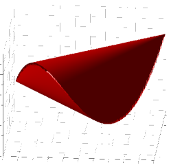
Figure 1: Representation of the unit PSD Toeplitz ball consisting of all $\left(x,y,z\right)$ such that $\boldsymbol{T}=\left[\begin{array}[]{cccc}1/4&x&y&z\\ x&1/4&x&y\\ y&x&1/4&x\\ z&y&x&1/4\end{array}\right]\succeq{\bf 0}$ and $\mathrm{Tr}\left(\boldsymbol{T}\right)=1$.

Encouragingly, the PSD Toeplitz cone can be very pointy around many low-rank feasible points, as illustrated in Fig. 1. Therefore, the intersection between the PSD Toeplitz cone and a random hyperplane passing through $\boldsymbol{\Sigma}$ often contains only a single point. As a result, the semidefinite relaxation (11) is exact with high probability under noise-free measurements, as stated in the following theorem.

Theorem 2.

Consider the sub-Gaussian sampling model in (4), and assume that $\mu_{4}\leq 3$ and $\left\|\boldsymbol{\eta}\right\|_{2}\leq\epsilon_{2}$. Then with probability exceeding $1-1/n^{2}$,

$$\|\hat{{\boldsymbol{\Sigma}}}-{\boldsymbol{\Sigma}}\|_{\mathrm{F}}\leq C_{2}\frac{\epsilon_{2}}{\sqrt{m}}$$ (12)

holds simultaneously for all Toeplitz covariance matrices $\boldsymbol{\Sigma}$ of rank at most $r$, provided that $m>c_{0}r\log^{10}n$. Here, $c_{0}$ and $C_{2}$ are some universal constants.

We highlight some implications of Theorem 2 as follows.

1. Exact Recovery without Noise. As any rank-$r$ PSD Toeplitz matrix admits a unique rank-$r$ Vandemonde decomposition that can be specified by $2r$ parameters, by Theorem 2, exact recovery of Toeplitz low-rank covariance matrices occurs as soon as $m$ is slightly larger than the information theoretic limit $\Omega\left(r\right)$ (modulo some poly-logarithmic factor). Note that this sampling requirement is much smaller than that for general low-rank matrices, and also much smaller than the degrees of freedom for general Toeplitz matrices (which is $n$).

2. Stable and Universal Recovery from Noisy Measurements. The proposed convex relaxation (11) returns faithful estimates in the presence of noise, as revealed by Theorem 2. This feature is universal: if $\mathcal{A}$ is randomly sampled and then fixed thereafter, then, with high probability, the error bounds (12) hold simultaneously for all Toeplitz low-rank matrices. Note that the error bound (12) is stated in terms of the $\ell_{2}$ norm of $\boldsymbol{\eta}$. This is out of mathematical convenience for this special setup, which will be discussed later.

Remark 2.

Two aspects of Theorem 2 are worth noting. First, Theorem 2 does not guarantee recovery with exponentially high probability as ensured in Theorem 1. This arises from our use of stochastic RIP, as will be seen in the analysis. Secondly, we are only able to provide theoretical guarantees when $\mu_{4}\leq 3$; roughly speaking, the tails of these distributions are typically not heavier than those of the Gaussian measure (e.g. $\mu_{4}=3$ for Gaussian distribution and $\mu_{4}=1$ for Bernoulli distribution). We conjecture that these two aspects can be improved via other proof techniques.

II-C Recovery of Sparse Covariance Matrices

Assume that $\boldsymbol{\Sigma}$ is approximately sparse, we propose to seek a matrix with minimal support size that is compatible with observations:

$$\hat{{\boldsymbol{\Sigma}}}=\operatorname{argmin}_{\boldsymbol{M}}\|\boldsymbol{M}\|_{0}\quad\text{subject to} \quad\boldsymbol{M}\succeq 0,$$ (13)

$$\quad\|{\boldsymbol{y}}-\mathcal{A}(\boldsymbol{M})\|_{1}\leq\epsilon_{1},$$

where $\epsilon_{1}$ is an upper bound on $\left\|\boldsymbol{\eta}\right\|_{1}$. However, the $\ell_{0}$ minimization problem in (13) is also intractable, and one can instead solve a tractable convex relaxation of (13), given as

$$\hat{{\boldsymbol{\Sigma}}}=\operatorname{argmin}_{\boldsymbol{M}}\|\boldsymbol{M}\|_{1}\quad\text{subject to} \quad\boldsymbol{M}\succeq 0,$$ (14)

$$\quad\|{\boldsymbol{y}}-\mathcal{A}(\boldsymbol{M})\|_{1}\leq\epsilon_{1}.$$

Here, the $\ell_{1}$ norm is the convex relaxation of the support size, which has proved successful in many compressed sensing algorithms [46, 32]. It turns out that the convex relaxation (14) allows stable and reliable estimates even when ${\boldsymbol{\Sigma}}$ is only approximately sparse and the measurements are contaminated by noise, as stated in the following theorem.

Theorem 3.

Consider the sub-Gaussian sampling model in (4) and assume that $\left\|\boldsymbol{\eta}\right\|_{1}\leq\epsilon_{1}$. Then with probability exceeding $1-C_{0}\exp(-c_{0}m)$, the solution $\hat{{\boldsymbol{\Sigma}}}$ to (14) satisfies

$$\|\hat{{\boldsymbol{\Sigma}}}-{\boldsymbol{\Sigma}}\|_{\mathrm{F}}\leq C_{1}\frac{\left\|{\boldsymbol{\Sigma}}-{\boldsymbol{\Sigma}}_{\Omega}\right\|_{1}}{\sqrt{k}}+C_{2}\frac{\epsilon_{1}}{m},$$ (15)

simultaneously for all $\boldsymbol{\Sigma}\in\mathbb{R}^{n\times n}$, provided that $m>c_{1}k\log(n^{2}/k)$. Here, ${\boldsymbol{\Sigma}}_{\Omega}$ denotes the best $k$-sparse approximation of ${\boldsymbol{\Sigma}}$, and $c_{0}$, $c_{1}$, $C_{0}$, $C_{1}$ and $C_{2}$ are positive universal constants.

Theorem 3 leads to similar implications as those listed in Section II-A, which we briefly summarize as follows.

1. Exact Recovery without Noise: When ${\boldsymbol{\Sigma}}$ is exactly $k$-sparse and no noise is present, by setting $\epsilon_{1}=0$, the solution to (14) is exactly equal to the ground truth with exponentially high probability, as soon as the number $m$ of measurements is about the order of $k\log(n^{2}/k)$. Therefore our performance guarantee in (15) is optimal within a constant factor.

2. Universal Recovery: Our performance guarantee in (15) is universal in the sense that the same sensing mechanism simultaneously works for all sparse covariance matrices.

3. Imperfect Structural Models: The estimate (15) allows robust recovery for approximately sparse matrices (which appears in a similar form as that for CS [46]), indicating that quadratic measurements are order-wise at least as good as linear measurements.

II-D Recovery of Jointly Sparse and Rank-One Matrices

If we set the covariance matrix ${\boldsymbol{\Sigma}}=\boldsymbol{x}\boldsymbol{x}^{\top}$ to be a rank-one matrix, then covariance estimation from quadratic measurements is equivalent to phase retrieval as studied in [15]. In addition to the general rank-one model, our approach allows simple analysis for recovering jointly sparse and rank-one covariance matrices or, equivalently, sparse signal recovery from magnitude measurements. Specifically, suppose that $\boldsymbol{x}$ is (approximately) sparse, and we collect a small number of phaseless measurements as

$$\boldsymbol{y}:=\left\{\left|\left\langle\boldsymbol{a}_{i},\boldsymbol{x}\right\rangle\right|^{2}+\eta_{i}\right\}_{1\leq i\leq m}.$$

When $\boldsymbol{x}$ is sparse, the lifting matrix $\boldsymbol{x}\boldsymbol{x}^{\top}$ is simultaneously low rank and sparse, which motivates us to adapt the convex program proposed in [24] to accommodate bounded noise as follows

$$\hat{\boldsymbol{X}}=\operatorname{argmin}_{\boldsymbol{M}}\quad \text{Tr}\left(\boldsymbol{M}\right)+\lambda\left\|\boldsymbol{M}\right\|_{1}$$ (16)

subject to $$\boldsymbol{M}\succeq 0,$$

$$\left\|\boldsymbol{y}-\mathcal{A}\left(\boldsymbol{M}\right)\right\|_{1}\leq\epsilon_{1}.$$

Here, $\lambda$ is a regularization parameter that balances the two convex surrogates (i.e. trace norm and $\ell_{1}$ norm) associated with the low-rank and sparse structural assumptions, respectively, and $\epsilon_{1}$ is an upper bound of $\left\|\boldsymbol{\eta}\right\|_{1}$. Our analysis framework ensures stable recovery of an approximately sparse signal, as stated in the following theorem.

Theorem 4.

Set $\lambda\in\left[\frac{1}{n},\frac{1}{\sqrt{k}}\rho\right]$ for some quantity $\rho$. Consider the sub-Gaussian sampling model in (4) and assume that $\left\|\boldsymbol{\eta}\right\|_{1}\leq\epsilon_{1}$. Then with probability at least $1-C_{0}\exp\left(-c_{0}m\right)$, the solution $\hat{\boldsymbol{X}}$ to (16) satisfies

$$\left\|\hat{\boldsymbol{X}}-\boldsymbol{x}\boldsymbol{x}^{\top}\right\|_{\mathrm{F}} \leq C_{1}\left\{\left\|\boldsymbol{x}\boldsymbol{x}^{\top}-\boldsymbol{x}_{\Omega}\boldsymbol{x}_{\Omega}^{\top}\right\|_{*}\right.$$

$$\quad\quad+\left.\lambda\left\|\boldsymbol{x}\boldsymbol{x}^{\top}-\boldsymbol{x}_{\Omega}\boldsymbol{x}_{\Omega}^{\top}\right\|_{1}+\frac{\epsilon_{1}}{m}\right\}$$ (17)

simultaneously for all signals $\boldsymbol{x}\in\mathbb{R}^{n}$ satisfying $\frac{\left\|\boldsymbol{x}_{\Omega}\right\|_{2}}{\left\|\boldsymbol{x}_{\Omega}\right\|_{1}}\geq\rho$, provided that $m>\frac{C_{2}\log n}{\lambda^{2}}$. Here, $\boldsymbol{x}_{\Omega}$ denotes the best $k$-sparse approximation of $\boldsymbol{x}$, and $C_{0}$, $C_{1},C_{2}$ and $c_{0}$ are positive universal constants.

Theorem 4, depending on the choice of $\lambda$, provides universal recovery guarantees over a large class of signals obeying $\frac{\left\|\boldsymbol{x}_{\Omega}\right\|_{2}}{\left\|\boldsymbol{x}_{\Omega}\right\|_{1}}\geq\rho$. Some implications of Theorem 4 are as follows.

1. Exact Recovery for Exactly Sparse Signals. When $\boldsymbol{x}$ is an exactly $k$-sparse signal, we can set $\rho=\frac{1}{\sqrt{k}}$ and $\lambda=\frac{1}{k}$ in Theorem 4, which implies the algorithm (16) universally recovers all $k$-sparse signals $\boldsymbol{x}$ from $O(k^{2}\log n)$ noise-free measurements, with exponentially high probability. This recovers the theoretical performance guarantees established in [24] for Gaussian sensing vectors, but extends it to a large class of sub-Gaussian sensing vectors, using a simpler proof.

2. Near-Optimal Recovery for Power-Law Exactly Sparse Signals. Somewhat surprisingly, if the nonzero entries of $\boldsymbol{x}$ are known to be decaying in a power-law fashion, then the algorithm (16) allows near-optimal recovery. Specifically, suppose that the non-zero entries of $\boldsymbol{x}$ satisfies the power-law decay such that the magnitude of the $l$th largest entry of $\boldsymbol{x}_{\Omega}/\left\|\boldsymbol{x}_{\Omega}\right\|_{2}$ is bounded above by ${c_{\text{pl}}}/{l^{\alpha}}$ for some constants $c_{\text{pl}}$ and exponent $\alpha>1$, then

   $$\|\boldsymbol{x}_{\Omega}\|_{2}/\|\boldsymbol{x}_{\Omega}\|_{1}=O\left(1/\log k\right):=\rho.$$

   By setting $\lambda=\Theta((\sqrt{k}\log n)^{-1})$, one can obtain accurate recovery from $O\left(k\log^{2}n\right)$ noiseless samples, which is only a logarithmic factor from the minimum sample complexity requirement.

3. Stable and Universal Recovery for Imperfect Models and Noisy Samples. When the sparsity assumption is inexact, or measurements are noisy, the estimate $\hat{\boldsymbol{X}}$ will not be exact, and we can recover the estimate of the signal $\hat{{\boldsymbol{x}}}$ as the top (normalized) eigenvector of $\hat{{\boldsymbol{X}}}$. Using the Davis-Kahan theorem in standard matrix perturbation theory [47], we have

   $$\sin\angle(\hat{{\boldsymbol{x}}},{\boldsymbol{x}})\leq\frac{1}{\|{\boldsymbol{x}}\|_{2}^{2}}\left\|\hat{\boldsymbol{X}}-\boldsymbol{x}\boldsymbol{x}^{\top}\right\|_{\mathrm{F}}$$

   bounded by Theorem 4, where $\angle(\hat{{\boldsymbol{x}}},{\boldsymbol{x}})$ represents the angle between $\hat{{\boldsymbol{x}}}$ and ${\boldsymbol{x}}$. The recovered signal $\hat{{\boldsymbol{x}}}$ is a highly accurate estimate if ${\boldsymbol{x}}_{\Omega^{c}}$ is small enough. The estimation inaccuracy due to noise corruption is also small, in the sense that it is at most proportional to the per-entry noise level. This generalizes prior work [24] to imperfect structural assumptions as well as noisy measurements.

II-E Extension to General Matrices

Table II summarizes the main results of Theorems 1 – 4. We further remark that the main results hold even when ${\boldsymbol{\Sigma}}$ is not PSD but a symmetric matrix. When ${\boldsymbol{\Sigma}}$ is not a covariance matrix but a general low-rank, Toeplitz low-rank, or sparse matrix, one can simply drop the PSD constraint in the proposed algorithms, and replace the trace norm objective by the nuclear norm in (7). As will be shown, the PSD constraint is never invoked in the proof, hence it is straightforward to extend all results to the more general cases where ${\boldsymbol{\Sigma}}$ is a general $n\times n$ low-rank, Toeplitz low-rank, or sparse matrix. Note that in this more general scenario, the measurements in (1) are no longer nonnegative.

TABLE II: Summary of Main Results.

Structure	Number of Measurements	Noise	RIP
rank-$r$	$O(nr)$	$\ell_{1}$	$\ell_{2}/\ell_{1}$
Toeplitz rank-$r$	$O(r\mbox{polylog}n)$	$\ell_{2}$	$\ell_{2}/\ell_{2}$
$k$-sparse	$O(k\log(n^{2}/k))$	$\ell_{1}$	$\ell_{2}/\ell_{1}$
$k$-sparse and rank-one	$O(k^{2}\log n)$ (general sparse);	$\ell_{1}$	$\ell_{2}/\ell_{1}$
	$O(k\log^{2}n)$ (power-law sparse)

III Approximate $\ell_{2}/\ell_{1}$ Isometry for Low-rank and Sparse Matrices

In this section, we present a novel concept called the mixed-norm restricted isometry property (RIP-$\ell_{2}/\ell_{1}$) that allows us to establish Theorems 1, 3, and 4 concerning universal recovery of low-rank, sparse and sparse rank-one covariance matrices from quadratic measurements.

Prevailing wisdom in CS asserts that perfect recovery from minimal samples is possible if the dimensionality reduction projection preserves the signal strength when acting on the class of matrices of interest [32, 44]. While there are various ways to define the restricted isometry properties (RIP), an appropriately chosen approximate isometry leads to a very simple yet powerful theoretical framework.

III-A Mixed-Norm Restricted Isometry (RIP-$\ell_{2}/\ell_{1}$)

Recall that the RIP occurs if the sampling output preserves the input strength under certain metrics. The most commonly used one is RIP-$\ell_{2}/\ell_{2}$, for which the signal strength before and after the projection are both measured in terms of the Frobenius norm [46, 44]. This, however, fails to hold under rank-one measurements – see detailed arguments by Candes et. al. in [15]. Another isometry concept called RIP-$\ell_{1}/\ell_{1}$ has also been investigated, for which the signal strength before and after the operation $\mathcal{A}$ are measured both in terms of the $\ell_{1}$ norms. This is initially developed to account for measurements from expander graphs [48], and has become a powerful metric when analyzing phase retrieval [15, 23, 24]. Nevertheless, when considering general low-rank matrices, RIP-$\ell_{1}/\ell_{1}$ no longer holds. To see this, consider two matrices

$$\boldsymbol{X}_{1} =\mbox{diag}\{\boldsymbol{I}_{r/2},\boldsymbol{I}_{r/2}{\bf 0}\}$$

$$\boldsymbol{X}_{2} =\mbox{diag}\{\boldsymbol{I}_{r/2},-\boldsymbol{I}_{r/2}{\bf 0}\}$$

enjoying the same nuclear norm. When $m=\Omega\left(nr\right)$, one can see from the Bernstein inequality (for sub-exponential variables) that

$$\frac{1}{m}\left\|\mathcal{A}\left(\boldsymbol{X}_{1}\right)\right\|_{1}=\Theta\left(r\right),\quad\frac{1}{m}\left\|\mathcal{A}\left(\boldsymbol{X}_{2}\right)\right\|_{1}=\Theta\left(\sqrt{r}\right),$$

precluding the existence of a small RIP-$\ell_{1}/\ell_{1}$ constant. Leaving out this matter, the proof based on RIP-$\ell_{1}/\ell_{1}$ typically relies on delicate construction of dual certificates [15, 23, 24], which is often mathematically complicated.

One of the key and novel ingredients in our analysis is a mixed-norm approximate isometry, which measures the signal strength before and after the projection with different metrics. Specifically, we introduce RIP-$\ell_{2}/\ell_{1}$, where the input and output are measured in terms of the Frobenius norm and the $\ell_{1}$ norm, respectively. It turns out that as long as the input is measured with the Frobenius norm, the standard trick pioneered in [46] in treating linear measurements carry over to quadratic measurements with slight modifications and saves the need for dual construction. We make formal definitions of RIP-$\ell_{2}/\ell_{1}$ for low-rank/sparse matrices as follows.

Definition 1 (RIP-$\ell_{2}/\ell_{1}$ for low-rank matrices).

For the set of rank-$r$ matrices, we define the RIP-$\ell_{2}/\ell_{1}$ constants $\delta_{r}^{\mathrm{lb}}$ and $\delta_{r}^{\mathrm{ub}}$ with respect to an operator $\mathcal{B}$ as the smallest numbers such that for all $\boldsymbol{X}$ of rank at most $r$:

$$\left(1-\delta_{r}^{\mathrm{lb}}\right)\left\|\boldsymbol{X}\right\|_{\mathrm{F}}\leq\frac{1}{m}\left\|\mathcal{B}\left(\boldsymbol{X}\right)\right\|_{1}\leq\left(1+\delta_{r}^{\mathrm{ub}}\right)\left\|\boldsymbol{X}\right\|_{\mathrm{F}}.$$

Definition 2 (RIP-$\ell_{2}/\ell_{1}$ for sparse matrices).

For the set of $k$-sparse matrices, we define the RIP-$\ell_{2}/\ell_{1}$ constants $\gamma_{k}^{\mathrm{lb}}$ and $\gamma_{k}^{\mathrm{ub}}$ with respect to an operator $\mathcal{B}$ as the smallest numbers such that for all $\boldsymbol{X}$ of sparsity at most $k$:

$$\left(1-\gamma_{k}^{\mathrm{lb}}\right)\left\|\boldsymbol{X}\right\|_{\mathrm{F}}\leq\frac{1}{m}\left\|\mathcal{B}\left(\boldsymbol{X}\right)\right\|_{1}\leq\left(1+\gamma_{k}^{\mathrm{ub}}\right)\left\|\boldsymbol{X}\right\|_{\mathrm{F}}.$$

Definition 3 (RIP-$\ell_{2}/\ell_{1}$ for low-rank plus sparse matrices).

Consider the class of index sets

$$\mathcal{S}_{k}: =\left\{\Omega\in[n]\times[n]\text{ }\Big{|}\text{ }\exists\text{ an index set }\omega\in[n]\right.$$

$$\quad\quad\quad\quad\quad\left.\text{ of cardinality }k\text{ such that }\Omega=\omega\times\omega\right\}.$$

For the set of matrices

$$\mathcal{M}_{k,r,l} =\left\{\boldsymbol{X}_{1}+\boldsymbol{X}_{2}\text{ }\Big{|}\text{ }\exists\Omega\in\mathcal{S}_{k},\text{ }\mathrm{rank}\left(\boldsymbol{X}_{1}\right)\leq r,\right.$$ (18)

$$\quad\quad\quad\quad\quad\quad\quad\left.\mathrm{supp}(\boldsymbol{X}_{1})\in\Omega,\text{ }\left\|\boldsymbol{X}_{2}\right\|_{0}\leq l\right\}.$$

we define the RIP-$\ell_{2}/\ell_{1}$ constants $\delta_{k,r,l}^{\mathrm{lb}}$ and $\delta_{k,r,l}^{\mathrm{ub}}$ with respect to an operator $\mathcal{B}$ as the smallest numbers such that $\forall\boldsymbol{X}\in\mathcal{M}_{k,r,l}$:

$$\left(1-\delta_{k,r,l}^{\mathrm{lb}}\right)\left\|\boldsymbol{X}\right\|_{\mathrm{F}}\leq\frac{1}{m}\left\|\mathcal{B}\left(\boldsymbol{X}\right)\right\|_{1}\leq\left(1+\delta_{k,r,l}^{\mathrm{ub}}\right)\left\|\boldsymbol{X}\right\|_{\mathrm{F}}.$$

Remark 3.

In short, any matrix within $\mathcal{M}_{k,r,l}$ can be decomposed into two components ${\boldsymbol{X}}_{1}$ and ${\boldsymbol{X}}_{2}$, where ${\boldsymbol{X}}_{1}$ is simultaneously low-rank and sparse, and ${\boldsymbol{X}}_{2}$ is sparse. This allows us to treat each matrix perturbation as a superposition of a collection of jointly low-rank and sparse matrices and a collection of general sparse matrices, where the rank-one measurements of each term can be well controlled under minimal sample complexity.

III-B RIP-$\ell_{2}/\ell_{1}$ of Quadratic Measurements for Low-rank and Sparse Matrices

Unfortunately, the original sampling operator $\mathcal{A}$ does not satisfy RIP-$\ell_{2}/\ell_{1}$. This occurs primarily because each measurement matrix $\boldsymbol{A}_{i}$ has non-zero mean, which biases the output measurements. In order to get rid of this undesired bias effect, we introduce a set of “debiased” auxiliary measurement matrices as follows

$$\boldsymbol{B}_{i}:=\boldsymbol{A}_{2i-1}-\boldsymbol{A}_{2i}.$$ (19)

Without loss of generality, denote $\mathcal{B}_{i}\left(\boldsymbol{X}\right):=\left\langle\boldsymbol{B}_{i},\boldsymbol{X}\right\rangle$ for all $1\leq i\leq m$, and let $\mathcal{B}\left(\boldsymbol{X}\right)$ represent the linear transformation that maps ${\boldsymbol{X}}$ to $\{\mathcal{B}_{i}\left(\boldsymbol{X}\right)\}_{i=1}^{m}$. Note that by representing the sensing process using $m$ rank-2 measurements $\mathcal{B}_{i}$, we have implicitly doubled the number of measurements for notational simplicity. This, however, will not change our order-wise results.

It turns out that the auxiliary operator $\mathcal{B}$ exhibits the RIP-$\ell_{2}/\ell_{1}$ in the presence of minimal measurements, which can be shown by combining the following proposition with a standard covering argument as applied in [49].

Proposition 1.

Let $\mathcal{A}$ be sampled from the sub-Gaussian model in (4). For any matrix ${\boldsymbol{X}}$, there exist universal constants $c_{1},c_{2},c_{3}>0$ such that with probability exceeding $1-\exp\left(-c_{3}m\right)$, one has

$$c_{1}\left\|\boldsymbol{X}\right\|_{\mathrm{F}}\leq\frac{1}{m}\left\|\mathcal{B}\left(\boldsymbol{X}\right)\right\|_{1}\leq c_{2}\left\|\boldsymbol{X}\right\|_{\mathrm{F}}.$$ (20)

Proof.

See Appendix A.∎

Remark 4.

This statement extends without difficulty to the bilinear rank-one measurement model where $\boldsymbol{y}_{i}=\boldsymbol{a}_{i}^{\top}{\boldsymbol{\Sigma}}\boldsymbol{b}_{i}$ for some independently generated sensing vectors $\boldsymbol{a}_{i}$ and $\boldsymbol{b}_{i}$. This indicates that all our results hold for this asymmetric sensing model as well.

An immediate consequence of Proposition 1 is the establishment of RIP-$\ell_{2}/\ell_{1}$ of the sampling operator $\mathcal{B}$ for either general low-rank or sparse matrices. The proof of the corollaries below follows immediately from a standard covering argument detailed in [49, Section III.B] and [50, Section 5]. We thus omit the details but refer interested readers to the above references for details.

Corollary 1 (RIP-$\ell_{2}/\ell_{1}$ for low-rank matrices).

Consider the sub-Gaussian sampling model in (4) and the universal constants $c_{1},c_{2}>0$ given in (20). There exist universal constants $c_{3},c_{4},C_{3}>0$ such that with probability exceeding $1-C_{3}\exp\left(-c_{3}m\right)$, $\mathcal{B}$ satisfies RIP-$\ell_{2}/\ell_{1}$ for all matrices $\boldsymbol{X}$ of rank at most $r$, and obeys

$$1-\delta_{r}^{\mathrm{lb}}\geq\frac{c_{1}}{2},\quad 1+\delta_{r}^{\mathrm{ub}}\leq 2c_{2},$$ (21)

provided that $m>c_{4}nr$.

Corollary 2 (RIP-$\ell_{2}/\ell_{1}$ for sparse matrices).

Consider the sub-Gaussian sampling model in (4) and the universal constants $c_{1},c_{2}>0$ given in (20). Then with probability exceeding $1-C_{3}\exp\left(-c_{3}m\right)$, $\mathcal{B}$ satisfies the RIP-$\ell_{2}/\ell_{1}$ for all matrices $\boldsymbol{X}$ of sparsity at most $k$, and obeys

$$1-\gamma_{k}^{\mathrm{lb}}\geq\frac{c_{1}}{2},\quad 1+\gamma_{k}^{\mathrm{ub}}\leq 2c_{2},$$ (22)

provided that $m>c_{4}k\log(n^{2}/k)$, where $c_{3},c_{4},C_{3}>0$ are some universal constants.

Corollary 3 (RIP-$\ell_{2}/\ell_{1}$ for low-rank plus sparse matrices).

Consider the sub-Gaussian sampling model in (4) and the universal constants $c_{1},c_{2}>0$ given in (20). Then with probability exceeding $1-C_{3}\exp\left(-c_{3}m\right)$, $\mathcal{B}$ satisfies the RIP-$\ell_{2}/\ell_{1}$ with respect to $\mathcal{M}_{k,r,l}$ (defined in (18)), and obeys

$$1-\delta_{k,r,l}^{\mathrm{lb}}\geq\frac{c_{1}}{2},\quad 1+\delta_{k,r,l}^{\mathrm{ub}}\leq 2c_{2},$$ (23)

provided that $m>c_{4}\max\left\{kr\log(n/k),l\log(n^{2}/l)\right\}$, where $c_{3},c_{4},C_{3}>0$ are some universal constants.

Remark 5.

Recall that each matrix in $\mathcal{M}_{k,r,l}$ is a sum of some $\boldsymbol{X}_{1}$ and $\boldsymbol{X}_{2}$, where $\boldsymbol{X}_{1}$ is a rank-$r$ matrix in a $k\times k$ subspace, while $\boldsymbol{X}_{2}$ is an $l$-sparse matrix. Consequently, if we let $\mathcal{C}_{\epsilon}\left(\mathcal{M}\right)$ stand for the covering number of a set $\mathcal{M}$ (i.e. the the fewest number of points in any $\epsilon$-net of $\mathcal{M}$), then $\mathcal{C}_{\epsilon}\left(\mathcal{M}_{k,r,l}\right)$ is apparently bounded above by the product of $\mathcal{C}_{\epsilon/2}\left(\mathcal{M}_{r}\right)$ and $\mathcal{C}_{\epsilon/2}\left(\mathcal{M}_{l}\right)$, where $\mathcal{M}_{r}$ and $\mathcal{M}_{l}$ denotes the rank-$r$ manifold (with ambient dimension $k$) and the $\ell$-sparse manifold (with ambient dimension $n^{2}$), respectively. Thus, $\log\mathcal{C}_{\epsilon}\left(\mathcal{M}_{k,r,l}\right)$ cannot exceed $kr\log(n/k)+l\log\left(n^{2}/l\right)$.

III-C Proof of Theorems 1, 3 and 4 via RIP-$\ell_{2}/\ell_{1}$

Theorems 1 and 3 can thus be proved given that the auxiliary operator $\mathcal{B}$ satisfies RIP-$\ell_{2}/\ell_{1}$ with sufficiently small constants, as asserted in Corollaries 1 and 2. We first present Lemma 1 which in turn establishes Theorem 1.

Lemma 1.

Consider any matrix ${\boldsymbol{\Sigma}}={\boldsymbol{\Sigma}}_{r}+{\boldsymbol{\Sigma}}_{\mathrm{c}}$, where ${\boldsymbol{\Sigma}}_{r}$ is the best rank-$r$ approximation of ${\boldsymbol{\Sigma}}$. If there exists a number $K_{1}>2r$ such that

$$\frac{1-\delta_{2r+K_{1}}^{\mathrm{lb}}}{\sqrt{2}}-\left(1+\delta_{K_{1}}^{\mathrm{ub}}\right)\sqrt{\frac{2r}{K_{1}}}\geq\beta_{1}>0$$ (24)

holds for some numerical value $\beta_{1}$, then the minimizer $\hat{{\boldsymbol{\Sigma}}}$ to (7) obeys

$$\|\hat{{\boldsymbol{\Sigma}}}-{\boldsymbol{\Sigma}}\|_{\mathrm{F}}\leq\left(\frac{C_{1}}{\beta_{1}}+C_{3}\right)\frac{\left\|{\boldsymbol{\Sigma}}_{\mathrm{c}}\right\|_{*}}{\sqrt{K_{1}}}+\frac{C_{2}}{\beta_{1}}\cdot\frac{\epsilon_{1}}{m}$$ (25)

for some positive universal constants $C_{1}$, $C_{2}$ and $C_{3}$ depending only on the RIP-$\ell_{2}/\ell_{1}$ constants.

Proof.

See Appendix C. ∎

By choosing

$$K_{1}=8\left(\frac{4c_{2}}{c_{1}}\right)^{2}r\geq 8\left(\frac{1+\delta_{K_{1}}^{\text{ub}}}{1-\delta_{2r+K_{1}}^{\text{ub}}}\right)^{2}r$$

for the universal constants $c_{1},c_{2}$ given in Corollary 1, we obtain (24) when $m>c_{4}\left(K_{1}+2r\right)n$ for some constant $c_{4}$. This establishes Theorem 1.

Theorem 3 is a direct consequence from the following lemma.

Lemma 2.

Consider any matrix ${\boldsymbol{\Sigma}}={\boldsymbol{\Sigma}}_{\Omega}+{\boldsymbol{\Sigma}}_{\Omega^{c}}$, where ${\boldsymbol{\Sigma}}_{\Omega}$ is the best $k$-term approximation of ${\boldsymbol{\Sigma}}$. If there exists a number $K_{2}>2k$ such that

$$\frac{(1-\gamma_{k+K_{2}}^{\mathrm{lb}})}{\sqrt{2}}-\left(1+\gamma_{K_{2}}^{\mathrm{ub}}\right)\sqrt{\frac{k}{K_{2}}}\geq\beta_{2}>0$$ (26)

holds for some numerical value $\beta_{2}$, then the minimizer $\hat{{\boldsymbol{\Sigma}}}$ to (7) obeys

$$\|\hat{{\boldsymbol{\Sigma}}}-{\boldsymbol{\Sigma}}\|_{\mathrm{F}}\leq\left(\frac{C_{1}}{\beta_{2}}+C_{3}\right)\frac{\left\|\boldsymbol{\Sigma}_{\Omega^{c}}\right\|_{1}}{\sqrt{K_{2}}}+\frac{C_{2}}{\beta_{2}}\frac{\epsilon_{1}}{m}$$ (27)

for some positive universal constants $C_{1}$, $C_{2}$, $C_{3}$ depending only on the RIP-$\ell_{2}/\ell_{1}$ constants.

Proof.

See Appendix D. ∎

By picking

$$K_{2}=4\left(\frac{4c_{2}}{c_{1}}\right)^{2}k\geq 4\left(\frac{1+\gamma_{K_{2}}^{\text{ub}}}{1-\gamma_{k+K_{2}}^{\text{lb}}}\right)^{2}k,$$

one obtains (26) as soon as $m>c_{4}\left(K_{2}+2k\right)\log(n^{2}/k)$ for the constant $c_{4}$ given in Corollary 2. This concludes the proof of Theorem 3.

Furthermore, the specialized RIP-$\ell_{2}/\ell_{1}$ concept allows us to prove Theorem 4 through the following lemma.

Lemma 3.

Set $\lambda$ to be any number within the interval $\left[\frac{1}{n},\frac{1}{\sqrt{k}}\frac{\left\|\boldsymbol{x}_{\Omega}\right\|_{2}}{\left\|\boldsymbol{x}_{\Omega}\right\|_{1}}\right]$. Suppose that $\boldsymbol{x}_{\Omega}$ is the best $k$-term approximation of $\boldsymbol{x}$. If there exists a number $K_{1}$ such that

$$\begin{cases}\frac{\frac{1}{\sqrt{3}}\left(1-\delta_{k,2K_{1},\frac{2K_{1}}{\lambda^{2}}}^{\mathrm{lb}}\right)-\frac{3}{\sqrt{K_{1}}}\left(1+\delta_{k,K_{1},\frac{K_{1}}{\lambda^{2}}}^{\mathrm{ub}}\right)}{2\max\left\{\frac{1}{\sqrt{K_{1}}}\left(1+\delta_{k,K_{1},\frac{K_{1}}{\lambda^{2}}}^{\mathrm{ub}}\right),1\right\}}\geq\beta_{3}>0,\\ \frac{1+\delta_{k,K_{1},\frac{K_{1}}{\lambda^{2}}}^{\mathrm{ub}}}{\left(1-\delta_{k,K_{1},\frac{K_{1}}{\lambda^{2}}}^{\mathrm{lb}}\right)\sqrt{K_{1}}}\leq\beta_{4}\end{cases}$$ (28)

for some absolute constants $\beta_{3}$ and $\beta_{4}$, then the solution $\hat{\boldsymbol{X}}$ to (16) satisfies

$$\left\|\hat{\boldsymbol{X}}-\boldsymbol{x}\boldsymbol{x}^{\top}\right\|_{\mathrm{F}} \leq C\left\{\left\|\boldsymbol{x}\boldsymbol{x}^{\top}-\boldsymbol{x}_{\Omega}\boldsymbol{x}_{\Omega}^{\top}\right\|_{*}\right.$$

$$\quad\quad\quad\left.+\lambda\left\|\boldsymbol{x}\boldsymbol{x}^{\top}-\boldsymbol{x}_{\Omega}\boldsymbol{x}_{\Omega}^{\top}\right\|_{1}+\frac{\epsilon_{1}}{m}\right\}$$ (29)

for some constant $C$ that depends only on $\beta_{3}$ and $\beta_{4}$.

Proof.

See Appendix E. ∎

From Corollary 3, one can ensure small RIP-$\ell_{2}/\ell_{1}$ constants satisfying (28), provided that

$$m>c_{4}\max\left\{kK_{1}\log n,\frac{K_{1}}{\lambda^{2}}\log n\right\}=c_{4}\frac{K_{1}}{\lambda^{2}}\log n.$$

This in turn establishes Theorem 4.

Finally, note that we have not discussed general Toeplitz low-rank matrices using RIP-$\ell_{2}/\ell_{2}$. We are unaware of a rigorous approach to prove exact recovery using RIP-$\ell_{2}/\ell_{1}$ for the Toeplitz case, partly due to the difficulty in characterizing the covering number for general low-rank Toeplitz matrices. Fortunately, the analysis for Toeplitz low-rank matrices can be performed by means of a different method, as detailed in the next section.

IV Approximate $\ell_{2}/\ell_{2}$ Isometry for Toeplitz Low-Rank Matrices

While quadratic measurements in general do not exhibit RIP-$\ell_{2}/\ell_{2}$ (as introduced in [44]) with respect to the set of general low-rank matrices (as pointed out in [15]), a slight variant of them can indeed satisfy RIP-$\ell_{2}/\ell_{2}$ when restricted to Toeplitz low-rank matrices. In this section, we first provide a characterization of RIP-$\ell_{2}/\ell_{2}$ for the set of general low-rank matrices under bounded and near-isotropic measurements, and then convert quadratic measurements into equivalent isotropic measurements.

IV-A RIP-$\ell_{2}/\ell_{2}$ for Near-Isotropic and Bounded Measurements

Before proceeding to the Toeplitz low-rank matrices, we investigate near-isotropic and bounded operators for the set of general low-rank matrices as follows. For convenience of presentation, we repeat the definition of RIP-$\ell_{2}/\ell_{2}$ as follows, followed by a theorem characterizing RIP-$\ell_{2}/\ell_{2}$ for near-isotropic and bounded operators.

Definition 4 (RIP-$\ell_{2}/\ell_{2}$ for low-rank matrices).

For the set of rank-$r$ matrices, we define the RIP-$\ell_{2}/\ell_{2}$ constants $\delta_{r}$ w.r.t. an operator $\mathcal{B}$ as the smallest number such that for all $\boldsymbol{X}$ of rank at most $r$,

$$\left(1-\delta_{r}\right)\left\|\boldsymbol{X}\right\|_{\mathrm{F}}\leq\frac{1}{m}\left\|\mathcal{B}\left(\boldsymbol{X}\right)\right\|_{2}\leq\left(1+\delta_{r}\right)\left\|\boldsymbol{X}\right\|_{\mathrm{F}}.$$

Theorem 5.

Suppose that for all $1\leq i\leq m$,

$$\left\|\boldsymbol{B}_{i}\right\|\leq K\quad\text{and}\quad\left\|\mathbb{E}\left[\mathcal{B}_{i}^{*}\mathcal{B}_{i}\right]-\mathcal{I}\right\|\leq\frac{c_{5}}{n}$$ (30)

hold for some quantity $K\leq n^{2}$. For any small constant $\delta>0$, if $m>c_{0}rK^{2}\log^{7}n$, then with probability at least $1-1/n^{2}$, one has

i) $\mathcal{B}$ satisfies RIP-$\ell_{2}/\ell_{2}$ w.r.t. all matrices of rank at most $r$ and obeys $\delta_{r}\leq\delta$;

ii) Suppose that $\mathcal{K}$ is some convex set. Then for all $\boldsymbol{\Sigma}$ of rank at most $r$ and $\boldsymbol{\Sigma}\in\mathcal{K}$, if $\left\|{\boldsymbol{y}}-\mathcal{B}(\boldsymbol{\Sigma})\right\|_{2}\leq\epsilon_{2}$, the solution

$$\hat{\boldsymbol{\Sigma}}=\operatorname{argmin}_{\boldsymbol{M}}\|\boldsymbol{M}\|_{*}\quad\mathrm{subject}\text{ }\mathrm{to}\quad \left\|{\boldsymbol{y}}-\mathcal{B}(\boldsymbol{M})\right\|_{2}\leq\epsilon_{2},$$

$$\boldsymbol{M}\in\mathcal{K},$$

satisfies

$$\|\hat{\boldsymbol{\Sigma}}-\boldsymbol{\Sigma}\|_{\mathrm{F}}\leq C_{2}\frac{\epsilon_{2}}{\sqrt{m}}$$ (31)

for some universal constants $c_{0},C_{2},c_{5}>0$.

Proof.

See Appendix B.∎

In fact, the bound on $\left\|\boldsymbol{B}_{i}\right\|$ can be as small as $\Theta\left(\sqrt{n}\right)$, and we say a measurement matrix $\boldsymbol{B}_{i}$ is well-bounded if $K=O\left(\sqrt{n}\mathrm{polylog}n\right)$. Simultaneously well-bounded and near-isotropic operators (i.e. those satisfying (30)) subsume the Fourier-type basis discussed in [26]. Theorem 5 strengthens the result in [26] to admit universal and stable recovery of low-rank matrices with random subsampling using Fourier-type basis, by justifying RIP-$\ell_{2}/\ell_{2}$ as soon as $m=\Omega\left(nr\mathrm{polylog}n\right)$.

Unfortunately, Theorem 5 cannot be directly applied to the class of Toeplitz low-rank matrices for the following reasons: i) The sampling operator $\mathcal{A}$ is neither isotropic nor well-bounded; ii) Theorem 5 requires $m=\Omega\left(nr\mathrm{polylog}n\right)$ measurements, which far exceeds the ambient dimension of a Toeplitz matrix, which is $n$. This motivates us to construct another set of equivalent sampling operators that satisfies the assumptions of Theorem 5, which is the focus of the following subsection.

IV-B Construction of RIP-$\ell_{2}/\ell_{2}$ Operators for Toeplitz Low-rank Matrices

Note that the quadratic measurement matrices $\boldsymbol{A}_{i}=\boldsymbol{a}_{i}\boldsymbol{a}_{i}^{\top}$ are neither non-isotropic nor well bounded. For instance, when $\boldsymbol{a}_{i}\sim\mathcal{N}\left(\boldsymbol{0},\boldsymbol{I}_{n}\right)$, simple calculation reveals that

$$\left\|\boldsymbol{A}_{i}\right\|=\Theta\left(\sqrt{n}\right),\quad\text{and}\quad\mathbb{E}\left[\boldsymbol{A}_{i}\left\langle\boldsymbol{A}_{i},\boldsymbol{X}\right\rangle\right]=2\boldsymbol{X}+\text{tr}\left(\boldsymbol{X}\right)\cdot\boldsymbol{I},$$ (32)

precluding $\boldsymbol{A}_{i}$’s from being isotropic. In order to facilitate the use of Theorem 5, we generate a new set of measurement matrices $\tilde{\boldsymbol{B}}_{i}$ through the following procedure.

1. Define a set of matrices $\boldsymbol{B}_{i}$ of rank at most 3

   $$\boldsymbol{B}_{i}:=\begin{cases}\frac{1}{2}\left(\boldsymbol{A}_{2i-1}-\boldsymbol{A}_{2i}\right),\quad&\text{if }\mu_{4}=3,\\ \alpha\boldsymbol{A}_{3i}+\beta\boldsymbol{A}_{3i-1}+\gamma\boldsymbol{A}_{3i-2},\quad&\text{if }\mu_{4}<3,\end{cases}$$ (33)

   where $\alpha,\beta,\gamma$ are specified in Lemma 4.

2. Generate $M$ (whose choice will be specified later) matrices independently such that

   $$\hat{\boldsymbol{B}}_{i}=\begin{cases}\sqrt{n}\mathcal{T}\left(\boldsymbol{B}_{i}\right),\quad&\text{with probability }\frac{1}{n},\\ \sqrt{\frac{n}{n-1}}\mathcal{T}^{\perp}\left(\boldsymbol{G}_{i}\right),&\text{with probability }\frac{n-1}{n},\end{cases}$$ (34)

   where $\boldsymbol{G}_{i}$ is a random matrix with i.i.d. standard Gaussian entries.

3. Define a truncated version $\tilde{\boldsymbol{B}}_{i}$ of $\hat{\boldsymbol{B}}_{i}$ as follows

   $$\tilde{\boldsymbol{B}}_{i}=\hat{\boldsymbol{B}}_{i}\cdot{1}_{\left\{\left\|\hat{\boldsymbol{B}}_{i}\right\|\leq c_{10}\log^{3/2}n\right\}},\quad 1\leq i\leq M.$$ (35)

We will demonstrate that the $\tilde{\boldsymbol{B}}_{i}$’s are nearly-isotropic and well-bounded, and hence by Theorem 5 the associated operator $\tilde{\mathcal{B}}$ enables exact and stable recovery for all rank-$r$ matrices when $M$ exceeds $O(nr\mathrm{polylog}n)$. This in turn establishes Theorem 2 through an equivalence argument, detailed later.

IV-B1 Isotropy Trick

While $\boldsymbol{A}_{i}$’s are in general non-isotropic, a linear combination of them can be made isotropic when restricted to Toeplitz matrices. This is stated in the following lemma.

Lemma 4.

Consider the sub-Gaussian sampling model in (4).

1) When $\mu_{4}=3$, then for any $\boldsymbol{X}$, the matrix

$$\boldsymbol{B}_{i}=\frac{1}{2}\left(\boldsymbol{A}_{2i-1}-\boldsymbol{A}_{2i}\right)$$ (36)

satisfies

$$\mathbb{E}\left[\boldsymbol{B}_{i}\left\langle\boldsymbol{B}_{i},\boldsymbol{X}\right\rangle\right]=\text{ }\boldsymbol{X}.$$ (37)

2) When $\mu_{4}<3$, take any constant $\xi>0$ obeying $\xi^{2}>1.5(3-\mu_{4})$ and set

$$\boldsymbol{B}_{i}=\alpha\boldsymbol{A}_{3i}+\beta\boldsymbol{A}_{3i-1}+\gamma\boldsymbol{A}_{3i-2},$$ (38)

with the choice of $\Delta:=-\left(1-\frac{\xi}{n}\right)^{2}-2+\frac{2\xi^{2}}{3-\mu_{4}}$,

$$\begin{cases}\alpha=\sqrt{\frac{3-\mu_{4}}{2\xi^{2}}},\\ \beta:=\frac{-\left(1-\frac{\xi}{\sqrt{n}}\right)+\sqrt{\Delta}}{2}\alpha,\\ \gamma:=\frac{-\left(1-\frac{\xi}{\sqrt{n}}\right)-\sqrt{\Delta}}{2}\alpha.\end{cases}$$ (39)

Then, for any norm $\left\|\cdot\right\|_{\mathrm{n}}$ and any $\boldsymbol{X}$ that satisfies $\boldsymbol{X}_{11}=\boldsymbol{X}_{22}=\cdots=\boldsymbol{X}_{nn}$, one has

$$\begin{cases}\mathbb{E}\left[\boldsymbol{B}_{i}\right]=\text{ }\sqrt{\frac{3-\mu_{4}}{2n}};\\ \mathbb{E}\left[\boldsymbol{B}_{i}\left\langle\boldsymbol{B}_{i},\boldsymbol{X}\right\rangle\right]=\text{ }\boldsymbol{X};\\ \left\|\boldsymbol{B}_{i}\right\|_{\mathrm{n}}\leq\sqrt{3}\max_{i:1\leq i\leq m}\left\|\boldsymbol{A}_{i}\right\|_{\mathrm{n}}.\end{cases}$$ (40)

Proof.

See Appendix F. ∎

Lemma 4 asserts that a large class of measurement matrices can be made isotropic when restricted to the class of matrices with identical diagonal entries (e.g. Toeplitz matrices). This immediately implies that the operator $\hat{\mathcal{B}}$ associated with $\hat{\boldsymbol{B}}_{i}$’s (defined in (34)) is isotropic. Specifically, for any symmetric $\boldsymbol{X}$,

$$\mathbb{E}\left[\hat{\boldsymbol{B}}_{i}\left\langle\hat{\boldsymbol{B}}_{i},\boldsymbol{X}\right\rangle\right]$$

$$\quad=\mathbb{E}\left[\mathcal{T}\left(\boldsymbol{B}_{i}\right)\left\langle\boldsymbol{B}_{i},\mathcal{T}\left(\boldsymbol{X}\right)\right\rangle\right]+\mathbb{E}\left[\mathcal{T}^{\perp}\left(\boldsymbol{G}_{i}\right)\left\langle\boldsymbol{G}_{i},\mathcal{T}^{\perp}\left(\boldsymbol{X}\right)\right\rangle\right]$$

$$\quad=\mathcal{T}\left(\mathbb{E}\left[\boldsymbol{B}_{i}\left\langle\boldsymbol{B}_{i},\mathcal{T}\left(\boldsymbol{X}\right)\right\rangle\right]\right)+\mathcal{T}^{\perp}\left(\mathbb{E}\left[\boldsymbol{G}_{i}\left\langle\boldsymbol{G}_{i},\mathcal{T}^{\perp}\left(\boldsymbol{X}\right)\right\rangle\right]\right)$$

$$\quad=\mathcal{T}\left(\mathcal{T}\left(\boldsymbol{X}\right)\right)+\mathcal{T}^{\perp}\left(\mathcal{T}^{\perp}\left(\boldsymbol{X}\right)\right)=\boldsymbol{X},$$

which follows since $\boldsymbol{B}_{i}$ and $\boldsymbol{G}_{i}$ are both isotropic matrices, a consequence of Lemma 4.

IV-B2 Truncation of $\hat{\mathcal{B}}$ is near-isotropic

The operators associated with $\hat{\boldsymbol{B}}_{i}$’s are in general not well-bounded. Fortunately, $\hat{\boldsymbol{B}}_{i}$’s are well-bounded with high probability, which comes from the following lemma whose proof can be found in Appendix G.

Lemma 5.

Consider a random vector $\boldsymbol{z}$ that follows the sub-Gaussian sampling model as described in (4). There exists an absolute constant $c_{10}>0$ such that

$$\left\|\mathcal{T}\left(\boldsymbol{z}\boldsymbol{z}^{\top}\right)\right\|\leq c_{12}\log^{\frac{3}{2}}n$$ (41)

holds with probability exceeding $1-n^{-10}$.

As $\left\|\boldsymbol{B}_{i}\right\|$ can be bounded above by $\max_{1\leq i\leq m}\left\|\boldsymbol{A}_{i}\right\|$ up to some constant factor, Lemma 5 reveals that $\left\|\mathcal{T}\left(\boldsymbol{B}_{i}\right)\right\|$ can be well controlled for sub-Gaussian vectors, i.e.

$$\left\|\mathcal{T}\left(\boldsymbol{B}_{i}\right)\right\|\leq c_{10}\log^{\frac{3}{2}}n,\quad 1\leq i\leq m$$ (42)

with probability exceeding $1-3n^{-8}$. Similarly, classical results in random matrices (e.g. [53]) assert that $\left\|\boldsymbol{G}_{i}\right\|$ can also be bounded above by $O\left(\sqrt{n}\log n\right)$ with overwhelming probability. These bounds taken collectively suggest that

$$\|\hat{\boldsymbol{B}}_{i}\|\leq K:=c_{10}\sqrt{n}\log^{\frac{3}{2}}n,\quad 1\leq i\leq m$$ (43)

for some constant $c_{10}>0$ with probability exceeding $1-n^{-7}$.

The above stochastic boundedness property motivates us to study the truncated version $\tilde{\boldsymbol{B}}_{i}$ of $\hat{\boldsymbol{B}}_{i}$ as defined in (35). Interestingly, $\tilde{\boldsymbol{B}}_{i}$ is near-isotropic, a consequence of the following lemma whose proof can be found in Appendix H.

Lemma 6.

Suppose that the restriction of $\mathcal{B}_{i}$ to Toeplitz matrices is isotropic. Consider any event $E$ obeying $\mathbb{P}\left(E\right)\geq 1-\frac{1}{n^{5}}.$ Then there is some constant $c_{5}>0$ such that

$$\left\|\mathbb{E}\left[\mathcal{T}\mathcal{B}_{i}^{*}\mathcal{B}_{i}\mathcal{T}{\bf 1}_{E}\right]-\mathcal{T}\right\|\leq\frac{c_{5}}{n^{2}}.$$ (44)

The truncated version of $\boldsymbol{G}_{i}$ can be easily bounded as in [52], which we omit for simplicity of presentation. This combined with (44) indicates that

$$\left\|\mathbb{E}\left[\tilde{\mathcal{B}}_{i}^{*}\tilde{\mathcal{B}}_{i}\right]-\mathcal{I}\right\|$$

$$\quad\leq\left\|\mathbb{E}\left[\mathcal{T}\mathcal{B}_{i}^{*}\mathcal{B}_{i}\mathcal{T}\right]-\mathcal{\mathcal{T}}\right\|+\left\|\mathbb{E}\left[\mathcal{T}^{\perp}\mathcal{G}_{i}^{*}\mathcal{G}_{i}\mathcal{T}^{\perp}\right]-\mathcal{\mathcal{T}}^{\perp}\right\|$$

$$\quad\leq\frac{c_{5}}{n}.$$

IV-C Proof of Theorem 2

So far we have demonstrated that $\tilde{\boldsymbol{B}}_{i}$’s are near-isotropic and satisfy $\|\tilde{\boldsymbol{B}}_{i}\|=O\left(\sqrt{n}\log^{\frac{3}{2}}n\right)$. Suppose that $\|\boldsymbol{y}-\tilde{\mathcal{B}}\left(\boldsymbol{\Sigma}\right)\|_{2}\leq\tilde{\epsilon}_{2}$. Theorem 5 implies that if $M$ exceeds $\Theta\left(nr\log^{10}(n)\right)$, then the solution to

$$\tilde{\boldsymbol{\Sigma}}:=\operatorname{argmin}_{\boldsymbol{M}}\left\|\boldsymbol{M}\right\|_{*}\quad\text{subject to } \|\boldsymbol{y}-\tilde{\mathcal{B}}\left(\boldsymbol{M}\right)\|_{2}\leq\tilde{\epsilon}_{2},$$

$$\boldsymbol{M}\text{ is Toeplitz},$$ (45)

satisfies

$$\left\|\boldsymbol{\Sigma}-\tilde{\boldsymbol{\Sigma}}\right\|_{\text{F}}\leq C_{2}\frac{\tilde{\epsilon}_{2}}{\sqrt{M}}$$ (46)

for the entire set of rank-$r$ matrices $\boldsymbol{\Sigma}$. Apparently, such low-rank manifolds subsume all rank-$r$ Toeplitz matrices as special cases. This claim in turn establishes Theorem 2 through the following argument:

1. From (34) and the Chernoff bound, $\tilde{\mathcal{B}}$ entails $\Theta\left(\frac{M}{n}\right)=\Theta\left(r\log^{10}n\right)$ independent copies of $\sqrt{n}\mathcal{T}\left(\boldsymbol{B}_{i}\right)$, and all other measurements are on the orthogonal complement of the Toeplitz space.

2. For any rank-$r$ Toeplitz matrix $\boldsymbol{\Sigma}$, the original $\mathcal{A}$ entails $m/3>\Theta\left(r\log^{10}n\right)$ measurement matrices of the form $\mathcal{T}\left(\boldsymbol{B}_{i}\right)$, and any non-Toeplitz component of $\boldsymbol{X}$ is perfectly known (i.e. equal to 0). This indicates that the convex program (11) is tighter than (45) when $\tilde{\epsilon}_{2}=\Theta\left(\sqrt{n}\epsilon_{2}\right)$, i.e. one can construct (via coupling) a new probability space over which if the solution $\tilde{\boldsymbol{\Sigma}}$ to (45) is exact and unique, then it will be the unique solution to (11) as well. This combined with the universal bound (46) establishes Theorem 2.

V Numerical Examples

To demonstrate the practical applicability of the proposed convex relaxation under quadratic sensing, in this section we present a variety of numerical examples for low-rank or sparse covariance matrix estimation.

V-A Recovery of Low-Rank Covariance Matrices

We conduct a series of Monte Carlo trials for various parameters. Specifically, we choose $n=50$, and for each $(m,r)$ pair, we repeat the following experiments 20 times. We generate ${\boldsymbol{\Sigma}}$, an $n\times n$ PSD matrix via $\boldsymbol{\Sigma}=\boldsymbol{L}\boldsymbol{L}^{\top}$, where $\boldsymbol{L}$ is a randomly generated $n\times r$ matrix with independent Gaussian components. The sensing vectors are generated as i.i.d. Gaussian vectors and Bernoulli vectors, and we obtain noiseless quadratic measurements $\boldsymbol{y}$. We use the off-the-shelf SDP solver SDPT3 with the modeling software CVX, and declare a matrix ${\boldsymbol{\Sigma}}$ to be recovered if the solution $\hat{{\boldsymbol{\Sigma}}}$ returned by the solver satisfies $\|\hat{\boldsymbol{\Sigma}}-\boldsymbol{\Sigma}\|_{\text{F}}/\|\boldsymbol{\Sigma}\|_{\text{F}}<10^{-3}$. Figure 2 illustrates the empirical probability of successful recovery in these Monte Carlo trials, which is reflected through the color of each cell. In order to compare the optimality of the practical performance, we also plot the information theoretic limit in red lines, i.e. the fundamental lower limit on $m$ required to recover all rank-$r$ matrices, which is $nr-r(r-1)/2$ in our case. It turns out that the practical phase transition curve is very close to the theoretic sampling limit, which demonstrates the optimality of our algorithm.

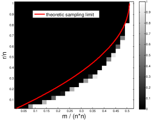
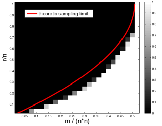
(a)	(b)

Figure 2: Recovery of covariance matrices from quadratic measurements when $n=50$. For each ($m,r$) pair, we repeated Monte Carlo trials 20 times. A PSD matrix ${\boldsymbol{\Sigma}}$ and $m$ sensing vectors are selected at random. The colormap for each cell indicates the empirical probability of success, and the red line reflects the fundamental information theoretic limit. The results are shown for (a) Gaussian sensing vectors and (b) symmetric Bernoulli sensing vectors.

In the second numerical example, we consider a random covariance matrix generated via the same procedure as above but with $n=40$. We let the rank $r$ vary as $1,3,5,10$ and the number of measurements $m$ vary from $20$ to $600$. For each pair of $(r,m)$, we perform $10$ independent experiments where in each run the sensing matrix is generated with i.i.d. Gaussian entries. Fig. 3 (a) shows the average Normalized Mean Squared Error (NMSE) defined as $\|\hat{\boldsymbol{\Sigma}}-\boldsymbol{\Sigma}\|_{\text{F}}^{2}/\|\boldsymbol{\Sigma}\|_{\text{F}}^{2}$ with respect to $m$ for different ranks when there is no noise. We further introduce additive bounded noise to each measurement by letting $\lambda_{i}$ be generated from $\sigma\cdot\mathcal{U}[-1,1]$, where $\mathcal{U}[-1,1]$ is a uniform distribution on $[-1,1]$, $\sigma$ is the noise level. Fig. 3 (b) shows the average NMSE when $r=5$ for different noise levels by setting $\epsilon=\sigma m$ in (7).

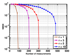
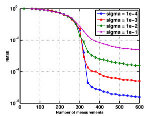
(a)	(b)

Figure 3: The NMSE of the reconstructed covariance matrix via trace minimization vs. the number of measurements when $n=40$: (a) for different ranks when no noise is present; (b) for different noise levels when $r=5$.

Interestingly, [23, 54] showed that when the covariance matrix is rank-one, if $m=O(n)$, the intersection of two convex sets, namely $\mathcal{S}_{1}=\{\boldsymbol{M}:\mathcal{A}(\boldsymbol{M})=\boldsymbol{y}\}$ and $\mathcal{S}_{2}=\{\boldsymbol{M}:\boldsymbol{M}\succ 0\}$ is a singleton, with high probability. For the low-rank case, if the same conclusion holds, we can find the solution via alternating projection between two convex sets. Therefore, we experiment on the following Projection Onto Convex Sets (POCS) procedure:

$$\boldsymbol{\Sigma}_{t+1}=\mathcal{P}_{\mathcal{S}_{2}}\mathcal{P}_{\mathcal{S}_{1}}\boldsymbol{\Sigma}_{t},$$ (47)

where $\mathcal{P}_{\mathcal{S}_{2}}$ denotes the projection onto the PSD cone, and

$$\mathcal{P}_{\mathcal{S}_{1}}\boldsymbol{\Sigma}_{t}:=\boldsymbol{\Sigma}_{t}-\mathcal{A}^{*}(\mathcal{A}\mathcal{A}^{*})^{-1}(\mathcal{A}(\boldsymbol{\Sigma_{t}})-\boldsymbol{y}).$$ (48)

Fig. 4 (a) shows the NMSE of the reconstruction with respect to the number of iterations for $r=3$ and different $m=200,250,300,350$. By comparing Fig. 3, we see that it requires more measurements for the POCS procedure to succeed, but the computational cost is much lower than the trace minimization. This is further validated from Fig. 4 (b), which is obtained under the same simulation setup as Fig. 3 by repeating POCS with $2000$ iterations.

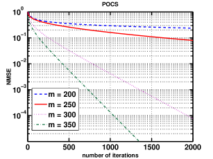
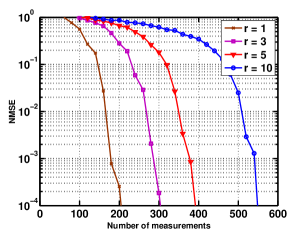
(a)	(b)

Figure 4: The NMSE of the reconstructed covariance matrix via POCS for $n=40$: (a) the NMSE vs. the number of iterations for different numbers of measurements when $r=3$; (b) the NMSE vs. the number of measurements for different ranks when running $2000$ iterations.

V-B Recovery of Toeplitz Low-rank Matrices

To justify the convex heuristic for Toeplitz low-rank matrices, we perform a series of numerical experiments for matrices of dimension $n=50$. By Caratheodory’s theorem, each PSD Toeplitz matrix can be uniquely decomposed into a linear combination of line spectrum [55]. Thus, we generate the PSD Toeplitz matrix by randomly generating the frequencies and amplitudes of each line spectra. In the real-valued case, the underlying spectral spikes occur in conjugate pairs (i.e. $\left(f_{1},-f_{1}\right),\left(f_{2},-f_{2}\right),\cdots$). We independently generate $r/2$ frequency pairs within the unit disk uniformly at random, and the amplitudes are generated as the absolute values of i.i.d. Gaussian variables. Figure 5 illustrates the phase transition diagram for varying choices of $(m,r)$. Each trial is declared successful if the estimate $\hat{\boldsymbol{\Sigma}}$ satisfies $\|\hat{\boldsymbol{\Sigma}}-\boldsymbol{\Sigma}\|_{\text{F}}/\left\|\boldsymbol{\Sigma}\right\|_{\text{F}}<10^{-3}.$ The empirical success rate is calculated by averaging over 50 Monte Carlo trials, and is reflected by the color of each cell. While there are in total $r$ degrees of freedom, our algorithm exhibits an approximately linear phase transition curve, which confirms our theoretical prediction in the absence of noise.

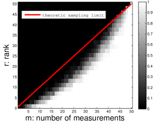
Figure 5: Phase transition plots where frequency locations are randomly generated. The plot corresponds to the situation where $n=50$. The empirical success rate is calculated by averaging over 50 Monte Carlo trials.

V-C Recovery of Sparse Matrices

We perform a series of Monte Carlo trials for various parameters for matrices of dimensions $50\times 50$. We first generate PSD sparse covariance matrices in the following way. For each sparsity value $k$, we generate a $\sqrt{k}\times\sqrt{k}$ matrix via $\boldsymbol{\Sigma}_{k}=\boldsymbol{L}\boldsymbol{L}^{\top}$, where $\boldsymbol{L}$ is a $\sqrt{k}\times\sqrt{k}$ matrix with independent Gaussian components. We then randomly select $\sqrt{k}$ rows and columns of ${\boldsymbol{\Sigma}}$ and embed ${\boldsymbol{\Sigma}}_{k}$ into the corresponding $\sqrt{k}\times\sqrt{k}$ submatrix; all other entries of ${\boldsymbol{\Sigma}}$ are set to 0. In addition, we also conduct numerical simulations for general symmetric sparse matrices, where the non-zero entries are drawn from an i.i.d. Gaussian distribution and the support is randomly chosen. For each $(m,k)$ pair in each scenario, we repeated the experiments 20 times, and solve it using CVX. Again, a matrix ${\boldsymbol{\Sigma}}$ is claimed to be recovered if the solution $\hat{{\boldsymbol{\Sigma}}}$ returned by the solver satisfies $\|\hat{\boldsymbol{\Sigma}}-\boldsymbol{\Sigma}\|_{\text{F}}/\|\boldsymbol{\Sigma}\|_{\text{F}}<10^{-3}$. Figure 6 illustrates the empirical success probability in these Monte Carlo experiments. For ease of comparison, we also plot the degrees of freedom in red lines, which is $\frac{\sqrt{k}\left(\sqrt{k}+1\right)}{2}$ in our case. It turns out that the practical phase transition curve is close to the theoretic sampling limit, which demonstrates the optimality of our algorithm.

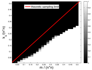
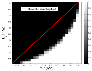
(a)	(b)

Figure 6: Reconstruction of sparse matrices from Gaussian quadratic measurements when $n=50$. For ease of comparison, we let $k_{\text{u}}$ denote the number of non-zero entries above or on the main diagonal, which represents the degrees of freedom for symmetric matrices. For each ($m,k_{\text{u}}$) pair, we conducted Monte Carlo experiments 20 times. A PSD matrix ${\boldsymbol{\Sigma}}$ and $m$ sensing vectors are selected at random. The colormap for each cell and the red line reflects the empirical probability of success and the information theoretic limit, respectively. The results are shown for (a) sparse PSD matrices, and (b) sparse symmetric matrices.

Another numerical example concerns recovery of a random symmetric sparse matrix (not necessarily PSD). We randomly generated a symmetric sparse matrix of sparsity level $k$ with $n=40$, and sketched it with i.i.d. Gaussian vectors. For each pair of $(r,m)$, we perform $10$ independent runs where in each run the sensing matrix is generated with i.i.d. standard Gaussian entries. Fig. 7 (a) shows the average NMSE with respect to $m$ for different sparsity levels when there is no noise. We further introduce additive bounded noise to each measurement by letting $\lambda_{i}$ be generated from $\sigma\cdot\mathcal{U}[-1,1]$, and run $10$ trials for each pair of $(\sigma,m)$. Fig. 7 (b) shows the average NMSE when $k=240$ for different noise levels by setting $\epsilon=\sigma m$ in (14).

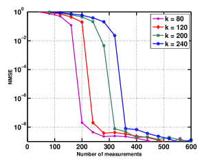
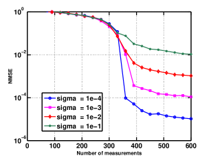
(a)	(b)

Figure 7: The NMSE of the reconstructed sparse matrix via $\ell_{1}$ minimization vs. the number of measurements when $n=40$: (a) for different sparsity level when no noise is present; (b) for different noise levels when $k=240$.

VI Conclusions and Future Work

We have investigated a general covariance estimation problem under a quadratic (rank-one) sampling model. This sampling model acts as an effective signal processing method for real-time data with limited processing power and memory at the data acquisition devices, and subsumes many sampling strategies where we can only obtain magnitude or energy samples. Three of the most popular covariance structures, i.e. sparsity, low rank, and jointly Toeplitz and low-rank structure, have been explored as well as sparse phase retrieval.

Our results indicate that covariance matrices under the above structural assumptions can be perfectly recovered from a small set of quadratic measurements and minimal storage, as long as the sensing vectors are i.i.d. drawn from sub-Gaussian distributions. The recovery can be achieved via efficient convex programming as soon as the memory complexity exceeds the fundamental sampling theoretic limit. We also observe universal recovery phenomena, in the sense that once the sensing vectors are chosen, all covariance matrices possessing the presumed structure can be recovered. Our results highlight the stability and robustness of the convex program in the presence of noise and imperfect structural assumptions. The performance guarantees for low-rank, sparse and jointly rank-one and sparse models are established via a novel notion of a mixed-norm restricted isometry property (RIP-$\ell_{2}/\ell_{1}$), which significantly simplifies the proof. Our contribution also includes a systematic approach to analyze Toeplitz low-rank structure, which relies on RIP-$\ell_{2}/\ell_{2}$ under near-isotropic and bounded operators.

Several future directions of interest are as follows.

• Another covariance structure of interest is an approximately sparse inverse covariance matrix rather than a sparse covariance matrix. In particular, when the signals are jointly Gaussian, the inverse covariance matrix encodes the conditional independence, which is often sparse. It remains to be seen whether the measurement scheme in (1) can be used to recover a sparse inverse covariance matrix.

• It will be interesting to explore whether more general types of sampling models satisfy RIP-$\ell_{2}/\ell_{1}$. For instance, when the sensing vectors do not have i.i.d. entries, more delicate mathematical tricks are necessary to establish RIP-$\ell_{2}/\ell_{1}$.

• In the case where RIP-$\ell_{2}/\ell_{1}$ is difficult to evaluate (e.g. the case with random Fourier sensing vectors), it would be interesting to develop an RIP-less theory in a similar flavor for linear measurement models [52].

Appendix A Proof of Proposition 1

To prove Proposition 1, we will first derive an upper bound and a lower bound on $\mathbb{E}\left[\left|\left\langle\boldsymbol{B}_{i},\boldsymbol{X}\right\rangle\right|\right]$, and then apply the Bernstein-type inequality [56, Proposition 5.16] to establish the large deviation bound.

In order to derive an upper bound on $\mathbb{E}\left[\left|\left\langle\boldsymbol{B}_{i},\boldsymbol{X}\right\rangle\right|\right]$, the key step is to apply the Hanson-Wright inequality [57, 58], which characterizes the concentration of measure for quadratic forms in sub-Gaussian random variables. We adopt the version in [58] and repeat it below for completeness.

Lemma 7 (Hanson-Wright Inequality).

Let ${\boldsymbol{X}}=(X_{1},\ldots,X_{n})\in\mathbb{R}^{n}$ be a random vector with independent components $X_{i}$ which satisfy $\mathbb{E}\left[X_{i}\right]=0$ and $\|X_{i}\|_{\psi_{2}}\leq K$. Let ${\boldsymbol{A}}$ be an $n\times n$ matrix. Then for any $t>0$,

$$\mathbb{P}\left\{\left|{\boldsymbol{X}}^{\top}{\boldsymbol{A}}{\boldsymbol{X}}-\mathbb{E}\left[{\boldsymbol{X}}^{\top}{\boldsymbol{A}}{\boldsymbol{X}}\right]\right|>t\right\}$$

$$\quad\leq 2\exp\left[-c\min\left(\frac{t^{2}}{K^{4}\|{\boldsymbol{A}}\|_{\mathrm{F}}^{2}},\frac{t}{K^{2}\|{\boldsymbol{A}}\|}\right)\right].$$ (49)

Remark 6.

Here, $\|\cdot\|_{\psi_{2}}$ denotes the sub-Gaussian norm

$$\|X\|_{\psi_{2}}:=\min_{p\geq 1}p^{-1/2}\left(\mathbb{E}\left[\left|X\right|^{p}\right]\right)^{1/p}.$$

Similarly, the sub-exponential norm $\|\cdot\|_{\psi_{1}}$ is defined as

$$\|X\|_{\psi_{1}}:=\min_{p\geq 1}p^{-1}\left(\mathbb{E}\left[\left|X\right|^{p}\right]\right)^{1/p}.$$

See [56, Section 5.2.3 and 5.2.4] for an introduction.

Observe that $\left\langle\boldsymbol{B}_{i},\boldsymbol{X}\right\rangle$ can be written as a symmetric quadratic form in $2n$ i.i.d. sub-Gaussian random variables

$$\left\langle\boldsymbol{B}_{i},\boldsymbol{X}\right\rangle=\begin{bmatrix}{\boldsymbol{a}}_{2i-1}^{\top}&{\boldsymbol{a}}_{2i}^{\top}\end{bmatrix}\begin{bmatrix}\boldsymbol{X}\\ &-\boldsymbol{X}\end{bmatrix}\begin{bmatrix}{\boldsymbol{a}}_{2i-1}\\ {\boldsymbol{a}}_{2i}\end{bmatrix}.$$

The Hanson-Wright inequality (49) then asserts that: there exists an absolute constant $c>0$ such that for any matrix $\boldsymbol{X}$, $\left|\left\langle\boldsymbol{B}_{i},\boldsymbol{X}\right\rangle\right|\leq t$ with probability at least

$$1-2\exp\left[-c\min\left(\frac{t^{2}}{4K^{4}\left\|\boldsymbol{X}\right\|_{\text{F}}^{2}},\frac{t}{K^{2}\left\|\boldsymbol{X}\right\|}\right)\right].$$

This indicates that $\left\langle\boldsymbol{B}_{i},\boldsymbol{X}\right\rangle$ is a sub-exponential random variable [56, Section 5.2.4] satisfying

$$\mathbb{E}\left[\left|\left\langle\boldsymbol{B}_{i},\boldsymbol{X}\right\rangle\right|\right]\leq c_{1}\left\|\boldsymbol{X}\right\|_{\text{F}}$$ (50)

for some positive constant $c_{1}$.

On the other hand, to derive a lower bound on $\mathbb{E}\left[\left|\left\langle\boldsymbol{B}_{i},\boldsymbol{X}\right\rangle\right|\right]$, we notice that for a random variable $\xi$, repeatedly applying the Cauchy-Schwartz inequality yields

$$\left(\mathbb{E}\left[\xi^{2}\right]\right)^{2}\leq\mathbb{E}\left[\left|\xi\right|\right]\mathbb{E}\left[\left|\xi\right|^{3}\right]\leq\mathbb{E}\left[\left|\xi\right|\right]\sqrt{\mathbb{E}\left[\xi^{2}\right]\mathbb{E}\left[\xi^{4}\right]},$$

which further leads to

$$\mathbb{E}\left[\left|\xi\right|\right]\geq\sqrt{\frac{\left(\mathbb{E}\left[\xi^{2}\right]\right)^{3}}{\mathbb{E}\left[\xi^{4}\right]}}.$$ (51)

Let $\xi:=\left\langle\boldsymbol{B}_{i},\boldsymbol{X}\right\rangle$, of which the second moment can be expressed as

$$\mathbb{E}\left[\xi^{2}\right]=\mathbb{E}\left[\left|\left\langle\boldsymbol{B}_{i},\boldsymbol{X}\right\rangle\right|^{2}\right]=\left\langle\boldsymbol{X},\mathbb{E}\left[\mathcal{B}_{i}^{*}\mathcal{B}_{i}\left(\boldsymbol{X}\right)\right]\right\rangle.$$

Simple algebraic manipulation yields

$$\mathbb{E}\left[\mathcal{B}_{i}^{*}\mathcal{B}_{i}\left(\boldsymbol{X}\right)\right]=4\boldsymbol{X}+2\left(\mu_{4}-3\right)\operatorname{diag}({\boldsymbol{X}}),$$

and hence

$$\mathbb{E}\left[\xi^{2}\right] =4\left\|\boldsymbol{X}\right\|_{\text{F}}^{2}+2\left(\mu_{4}-3\right)\sum_{i=1}^{n}\left|\boldsymbol{X}_{ii}\right|^{2}$$

$$\geq\min\{4,2(\mu_{4}-1)\}\left\|\boldsymbol{X}\right\|_{\text{F}}^{2}=c_{2}\left\|\boldsymbol{X}\right\|_{\text{F}}^{2},$$ (52)

where $c_{2}:=\min\{4,2(\mu_{4}-1)\}$. Furthermore, since $\xi:=\left\langle\boldsymbol{B}_{i},\boldsymbol{X}\right\rangle$ has been shown to be sub-exponential with sub-exponential norm $\Theta\left(\left\|\boldsymbol{X}\right\|_{\text{F}}\right)$, one can derive [56]

$$\mathbb{E}\left[\xi^{4}\right]=\left(4\left\|\xi\right\|_{\psi_{1}}\right)^{4}\leq c_{3}\left\|\boldsymbol{X}\right\|_{\text{F}}^{4}$$ (53)

for some constant $c_{7}>0$. This taken collectively with (51) and (52) gives rise to

$$\mathbb{E}\left[\left|\left\langle\boldsymbol{B}_{i},\boldsymbol{X}\right\rangle\right|\right]\geq\sqrt{\frac{c_{2}^{3}\left\|\boldsymbol{X}\right\|_{\text{F}}^{6}}{c_{3}\left\|\boldsymbol{X}\right\|_{\text{F}}^{4}}}=c_{4}\left\|\boldsymbol{X}\right\|_{\text{F}}$$

for some constant $c_{4}>0$.

Now, we are ready to characterize the concentration of $\left\langle\boldsymbol{B}_{i},\boldsymbol{X}\right\rangle$, which is a simple consequence of the following sub-exponential variant of Bernstein inequality.

Lemma 8 ([56, Proposition 5.16]).

Let $X_{1},\ldots,X_{m}$ be independent sub-exponential random variables with $\mathbb{E}\left[X_{i}\right]=0$ and $K=\max_{i}\|X_{i}\|_{\psi_{1}}$. Then for every $t>0$, we have

$$\mathbb{P}\left\{\frac{1}{m}\left|\sum_{i=1}^{m}X_{i}\right|\geq t\right\}\leq 2\exp\left[-cm\min\left(\frac{t^{2}}{K^{2}},\frac{t}{K}\right)\right]$$ (54)

where $c$ is an absolute constant.

Recall that it has been shown in (50) that the sub-exponential norm of $X_{i}:=\left|\left\langle\boldsymbol{B}_{i},\boldsymbol{X}\right\rangle\right|-\mathbb{E}\left[\left|\left\langle\boldsymbol{B}_{i},\boldsymbol{X}\right\rangle\right|\right]$ satisfies $\|X_{i}\|_{\psi_{1}}\leq c^{\prime}\|{\boldsymbol{X}}\|_{\mathrm{F}}$ for some universal constant $c^{\prime}$. Therefore, Lemma 8 implies that for any $\epsilon>0$, one has

$$\left|\frac{1}{m}\left\|\mathcal{B}({\boldsymbol{X}})\right\|_{1}-\frac{1}{m}\mathbb{E}\left[\left\|\mathcal{B}\left(\boldsymbol{X}\right)\right\|_{1}\right]\right|\leq\epsilon\|{\boldsymbol{X}}\|_{\text{F}}$$

with probability exceeding $1-2\exp(-cm\epsilon)$ for some absolute constant $c>0$. This yields

$$\frac{1}{m}\left\|\mathcal{B}({\boldsymbol{X}})\right\|_{1}\leq\frac{1}{m}\mathbb{E}\left[\left\|\mathcal{B}\left(\boldsymbol{X}\right)\right\|_{1}\right]+\epsilon\|{\boldsymbol{X}}\|_{\text{F}}\leq(c_{1}+\epsilon)\|{\boldsymbol{X}}\|_{\text{F}}$$

and

$$\frac{1}{m}\left\|\mathcal{B}({\boldsymbol{X}})\right\|_{1}\geq\frac{1}{m}\mathbb{E}\left[\left\|\mathcal{B}\left(\boldsymbol{X}\right)\right\|_{1}\right]-\epsilon\|{\boldsymbol{X}}\|_{\text{F}}\geq(c_{4}-\epsilon)\|{\boldsymbol{X}}\|_{\text{F}}$$

with probability at least $1-2\exp(-cm\epsilon)$, where the constants $c$, $c_{1}$ and $c_{4}$ depend only on the sub-Gaussian norm of $a_{i}$. Renaming the universal constants establishes Proposition 1.

Appendix B Proof of Theorem 5

The proof of Theorem 5 follows the entropy method introduced in [25] for compressed sensing and [27] for Pauli measurements. Note, however, that in our case, the measurement measurements do not form a basis, and are not even bounded. Our theorem extend the results in [27] (which focuses on Pauli basis) to general near-isotropic measurements.

Specifically, the RIP-$\ell_{2}/\ell_{2}$ constant can be bounded by

$$\delta_{r} =\sup_{\left\|\boldsymbol{X}\right\|_{\text{F}}\leq 1,\mathrm{rank}\left(\boldsymbol{X}\right)\leq r}\left|\frac{1}{m}\sum_{i=1}^{m}\left|\left\langle\boldsymbol{B}_{i},\boldsymbol{X}\right\rangle\right|^{2}-\left\|\boldsymbol{X}\right\|_{\mathrm{F}}^{2}\right|$$

$$=\sup_{T\in\mathcal{M}_{r}^{\mathrm{t}},\boldsymbol{X}\in T,\left\|\boldsymbol{X}\right\|_{\text{F}}\leq 1}\left|\left\langle\boldsymbol{X},\left(\frac{1}{m}\sum_{i=1}^{m}\mathcal{B}_{i}^{*}\mathcal{B}_{i}-\mathcal{I}\right)\boldsymbol{X}\right\rangle\right|$$ (55)

$$\leq\sup_{T\in\mathcal{M}_{r}^{\mathrm{t}}}\left\|\mathcal{P}_{T}\left(\frac{1}{m}\sum_{i=1}^{m}\mathcal{B}_{i}^{*}\mathcal{B}_{i}-\mathcal{I}\right)\mathcal{P}_{T}\right\|$$

$$\leq\sup_{T\in\mathcal{M}_{r}^{\mathrm{t}}}\left\|\mathcal{P}_{T}\left\{\frac{1}{m}\sum_{i=1}^{m}\left(\mathcal{B}_{i}^{*}\mathcal{B}_{i}-\mathbb{E}\mathcal{B}_{i}^{*}\mathcal{B}_{i}\right)\right\}\mathcal{P}_{T}\right\|+\frac{c_{5}}{n},$$ (56)

where

$$\mathcal{M}_{r}^{\mathrm{t}}:=\left\{\text{tangent space w.r.t. }\boldsymbol{M}\mid\forall\boldsymbol{M}:\text{ }\text{rank}\left(\boldsymbol{M}\right)\leq r\right\}.$$ (57)

and hence (55) arises since the supremum is taken over all tangent space $T$ associated with rank-$r$ matrices. The last inequality (56) follows from the near-isotropic assumption of $\mathcal{B}_{i}$ (i.e. (30)).

The first step is to prove that $\mathbb{E}\left[\delta_{r}\right]\leq\epsilon$ for some small constant $\epsilon>0$. For sufficiently large $n$, it suffices to prove that

$$E:=\mathbb{E}\left[\sup_{T\in\mathcal{M}_{r}^{\mathrm{t}}}\left\|\mathcal{P}_{T}\left\{\frac{1}{m}\sum_{i=1}^{m}\left(\mathcal{B}_{i}^{*}\mathcal{B}_{i}-\mathbb{E}\left[\mathcal{B}_{i}^{*}\mathcal{B}_{i}\right]\right)\right\}\mathcal{P}_{T}\right\|\right]\leq\delta.$$ (58)

This can be established by a Gaussian process approach as follows.

Observe that $\frac{1}{m}\sum_{i=1}^{m}\left(\mathcal{B}_{i}^{*}\mathcal{B}_{i}-\mathbb{E}\left[\mathcal{B}_{i}^{*}\mathcal{B}_{i}\right]\right)$ is a zero-mean operator, which can be reduced to symmetric operators via the symmetrization argument (see, e.g. [53]). Specifically, let $\tilde{\mathcal{B}}_{i}$ be an independent copy of $\mathcal{B}_{i}$. Conditioning on $\mathcal{B}_{i}$ we have

$$\mathbb{E}\left[\left.\frac{1}{m}\sum_{i=1}^{m}\mathcal{B}_{i}^{*}\mathcal{B}_{i}-\frac{1}{m}\sum_{i=1}^{m}\tilde{\mathcal{B}}_{i}^{*}\tilde{\mathcal{B}}_{i}\right|\mathcal{B}_{i}\text{ }(1\leq i\leq m)\right]$$

$$\quad=\frac{1}{m}\sum_{i=1}^{m}\mathcal{B}_{i}^{*}\mathcal{B}_{i}-\mathbb{E}\left[\mathcal{B}_{i}^{*}\mathcal{B}_{i}\right].$$

Since the function $f\left(\mathcal{X}\right):=\sup_{T\in\mathcal{M}_{r}^{\mathrm{t}}}\left\|\mathcal{P}_{T}\mathcal{X}\mathcal{P}_{T}\right\|$ is convex in $\mathcal{X}$, applying Jensen’s inequality yields

$$\sup_{T\in\mathcal{M}_{r}^{\mathrm{t}}}\left\|\mathcal{P}_{T}\left\{\frac{1}{m}\sum_{i=1}^{m}\left(\mathcal{B}_{i}^{*}\mathcal{B}_{i}-\mathbb{E}\left[\mathcal{B}_{i}^{*}\mathcal{B}_{i}\right]\right)\right\}\mathcal{P}_{T}\right\|$$

$$\text{ }\text{ }\footnotesize=\sup_{T\in\mathcal{M}_{r}^{\mathrm{t}}}\left\|\mathbb{E}\left[\left.\mathcal{P}_{T}\left(\frac{1}{m}\sum_{i=1}^{m}\mathcal{B}_{i}^{*}\mathcal{B}_{i}-\frac{1}{m}\sum_{i=1}^{m}\tilde{\mathcal{B}}_{i}^{*}\tilde{\mathcal{B}}_{i}\right)\mathcal{P}_{T}\right|\mathcal{B}_{i}\right]\right\|$$

$$\text{ }\text{ }\footnotesize\leq\text{ }\mathbb{E}\left[\left.\sup_{T\in\mathcal{M}_{r}^{\mathrm{t}}}\left\|\mathcal{P}_{T}\left(\frac{1}{m}\sum_{i=1}^{m}\mathcal{B}_{i}^{*}\mathcal{B}_{i}-\frac{1}{m}\sum_{i=1}^{m}\tilde{\mathcal{B}}_{i}^{*}\tilde{\mathcal{B}}_{i}\right)\mathcal{P}_{T}\right\|\right|\mathcal{B}_{i}\right].$$

Undoing conditioning over $\mathcal{B}_{i}$ we get

$$\mathbb{E}\left[\sup_{T\in\mathcal{M}_{r}^{\mathrm{t}}}\left\|\mathcal{P}_{T}\left\{\frac{1}{m}\sum_{i=1}^{m}\left(\mathcal{B}_{i}^{*}\mathcal{B}_{i}-\mathbb{E}\left[\mathcal{B}_{i}^{*}\mathcal{B}_{i}\right]\right)\right\}\mathcal{P}_{T}\right\|\right]$$

$$\quad\leq\text{ }\mathbb{E}\left[\sup_{T\in\mathcal{M}_{r}^{\mathrm{t}}}\left\|\mathcal{P}_{T}\left(\frac{1}{m}\sum_{i=1}^{m}\mathcal{B}_{i}^{*}\mathcal{B}_{i}-\frac{1}{m}\sum_{i=1}^{m}\tilde{\mathcal{B}}_{i}^{*}\tilde{\mathcal{B}}_{i}\right)\mathcal{P}_{T}\right\|\right]$$

$$\quad\leq\text{ }2\mathbb{E}\left[\sup_{T\in\mathcal{M}_{r}^{\mathrm{t}}}\left\|\frac{1}{m}\sum_{i=1}^{m}\epsilon_{i}\mathcal{P}_{T}\mathcal{B}_{i}^{*}\mathcal{B}_{i}\mathcal{P}_{T}\right\|\right],$$ (59)

where $\epsilon_{i}$’s are i.i.d. symmetric Bernoulli random variables. Moreover, if we generate a set of i.i.d. random variables $g_{i}\sim\mathcal{N}\left(0,1\right)$, then the conditional expectation obeys

$$\mathbb{E}\left[\left.\frac{1}{m}\sum_{i=1}^{m}\left|g_{i}\right|\epsilon_{i}\mathcal{P}_{T}\mathcal{B}_{i}^{*}\mathcal{B}_{i}\mathcal{P}_{T}\right|\epsilon_{i},\mathcal{B}_{i}\right]$$

$$\quad=\sqrt{\frac{2}{\pi}}\frac{1}{m}\sum_{i=1}^{m}\epsilon_{i}\mathcal{P}_{T}\mathcal{B}_{i}^{*}\mathcal{B}_{i}\mathcal{P}_{T}.$$

Similarly, by convexity of $f\left(\mathcal{X}\right):=\sup_{T\in\mathcal{M}_{r}^{\mathrm{t}}}\left\|\mathcal{P}_{T}\mathcal{X}\mathcal{P}_{T}\right\|$, one can obtain

$$\mathbb{E}\left[\sup_{T\in\mathcal{M}_{r}^{\mathrm{t}}}\left\|\frac{1}{m}\sum_{i=1}^{m}\epsilon_{i}\mathcal{P}_{T}\mathcal{B}_{i}^{*}\mathcal{B}_{i}\mathcal{P}_{T}\right\|\right]$$

$$\text{ }\text{ }=\sqrt{\frac{\pi}{2}}\mathbb{E}\left[\sup_{T\in\mathcal{M}_{r}^{\mathrm{t}}}\left\|\mathbb{E}\left[\left.\frac{1}{m}\sum_{i=1}^{m}\left|g_{i}\right|\epsilon_{i}\mathcal{P}_{T}\mathcal{B}_{i}^{*}\mathcal{B}_{i}\mathcal{P}_{T}\right|\epsilon_{i},\mathcal{B}_{i}\right]\right\|\right]$$

$$\text{ }\text{ }\leq\sqrt{\frac{\pi}{2}}\mathbb{E}\left[\sup_{T\in\mathcal{M}_{r}^{\mathrm{t}}}\left\|\frac{1}{m}\sum_{i=1}^{m}g_{i}\mathcal{P}_{T}\mathcal{B}_{i}^{*}\mathcal{B}_{i}\mathcal{P}_{T}\right\|\right].$$ (60)

Putting (59) and (60) together we obtain

$$\mathbb{E}\left[\sup_{T\in\mathcal{M}_{r}^{\mathrm{t}}}\left\|\mathcal{P}_{T}\left\{\frac{1}{m}\sum_{i=1}^{m}\left(\mathcal{B}_{i}^{*}\mathcal{B}_{i}-\mathbb{E}\left[\mathcal{B}_{i}^{*}\mathcal{B}_{i}\right]\right)\right\}\mathcal{P}_{T}\right\|\right]$$

$$\quad\leq\sqrt{2\pi}\mathbb{E}\left[\sup_{T\in\mathcal{M}_{r}^{\mathrm{t}}}\left\|\frac{1}{m}\sum_{i=1}^{m}g_{i}\mathcal{P}_{T}\mathcal{B}_{i}^{*}\mathcal{B}_{i}\mathcal{P}_{T}\right\|\right]$$

$$\quad=\sqrt{2\pi}\mathbb{E}\left[\sup_{T\in\mathcal{M}_{r}^{\mathrm{t}},\boldsymbol{X}\in T,\left\|\boldsymbol{X}\right\|_{\text{F}}=1}\left|\frac{1}{m}\sum_{i=1}^{m}g_{i}\left|\mathcal{B}_{i}\left(\boldsymbol{X}\right)\right|^{2}\right|\right].$$ (61)

It then boils down to characterizing the supremum of a Gaussian process.

We now prove the following lemma.

Lemma 9.

Suppose that $g_{i}\sim\mathcal{N}(0,1)$ are i.i.d. random variables, and that $K\leq n^{2}$. Conditional on $\mathcal{B}_{i}$’s, we have

$$\mathbb{E}\left[\left.\sup_{T\in\mathcal{M}_{r}^{\mathrm{t}}}\Bigg{\|}\mathcal{P}_{T}\left(\sum_{i=1}^{m}g_{i}\mathcal{B}_{i}^{*}\mathcal{B}_{i}\right)\mathcal{P}_{T}\Bigg{\|}\text{ }\right|\mathcal{B}_{i}\text{ }(1\leq i\leq m)\right]$$

$$\quad\leq C_{14}\sqrt{r}K\log^{3}n\sup_{T:T\in\mathcal{M}_{r}^{\mathrm{t}}}\sqrt{\left\|\sum_{i=1}^{m}\mathcal{P}_{T}\mathcal{B}_{i}^{*}\mathcal{B}_{i}\mathcal{P}_{T}\right\|}.$$ (62)

Proof.

See Appendix I.∎

Combining Lemma 9 with (61) and undoing the conditioning on $\mathcal{B}_{i}$’s yield

$$\mathbb{E}\left[\sup_{T\in\mathcal{M}_{r}^{\mathrm{t}}}\left\|\mathcal{P}_{T}\left\{\frac{1}{m}\sum_{i=1}^{m}\left(\mathcal{B}_{i}^{*}\mathcal{B}_{i}-\mathbb{E}\mathcal{B}_{i}^{*}\mathcal{B}_{i}\right)\right\}\mathcal{P}_{T}\right\|\right]$$

$$\quad\leq\text{ }\frac{C_{15}\sqrt{r}K\log^{3}n}{m}\cdot\mathbb{E}\left[\sqrt{\sup_{T:T\in\mathcal{M}_{r}^{\mathrm{t}}}\left\|\sum_{i=1}^{m}\mathcal{P}_{T}\mathcal{B}_{i}^{*}\mathcal{B}_{i}\mathcal{P}_{T}\right\|}\right]$$

$$\quad\leq\frac{C_{15}\sqrt{r}K\log^{3}n}{\sqrt{m}}\sqrt{\mathbb{E}\left[\sup_{T:T\in\mathcal{M}_{r}^{\mathrm{t}}}\left\|\frac{1}{m}\sum_{i=1}^{m}\mathcal{P}_{T}\mathcal{B}_{i}^{*}\mathcal{B}_{i}\mathcal{P}_{T}\right\|\right]}$$

for some universal constant $C_{15}>0$, where the last inequality follows from Jensen’s inequality. Recall the definition of $E$ in (58), then the above inequality implies

$$E\leq C_{15}\left(\frac{\sqrt{r}K\log^{3}n}{\sqrt{m}}\right)\sqrt{E+1},$$

or more concretely,

$$\mathbb{E}\left[\delta_{r}\right]\leq E\leq 2C_{15}\frac{\sqrt{r}K\log^{3}n}{\sqrt{m}}<1$$ (63)

as soon as $m>\left(2C_{15}\sqrt{r}K\log^{3}n\right)^{2}$.

Now that we have established that $\mathbb{E}\left[\delta_{r}\right]$ can be a small constant if $m>4C_{15}^{2}rK^{2}\log^{6}n$, it remains to show that $\delta_{r}$ sharply concentrates around $\mathbb{E}\sigma_{r}$. To this end, consider the Banach space $\Upsilon$ of operators $\mathcal{H}:\mathbb{R}^{n\times n}\mapsto\mathbb{R}^{n\times n}$ equipped with the norm

$$\left\|\mathcal{H}\right\|_{\Upsilon}:=\sup_{T\in\mathcal{M}_{r}^{\mathrm{t}}}\left\|\mathcal{P}_{T}\mathcal{H}\mathcal{P}_{T}\right\|.$$

Let $\varepsilon_{i}$’s be i.i.d. symmetric Bernoulli variables, then the symmetrization trick (see, e.g. [53]) yields

$$\mathbb{E}\left[\left\|\frac{1}{m}\sum_{i=1}^{m}\mathcal{B}_{i}^{*}\mathcal{B}_{i}-\mathbb{E}\left[\mathcal{B}_{i}^{*}\mathcal{B}_{i}\right]\right\|_{\Upsilon}\right]$$

$$\quad\leq\mathbb{E}\left[\left\|\frac{1}{m}\sum_{i=1}^{m}\varepsilon_{i}\mathcal{B}_{i}^{*}\mathcal{B}_{i}\right\|_{\Upsilon}\right]$$

$$\quad\leq 2\mathbb{E}\left\|\frac{1}{m}\sum_{i=1}^{m}\mathcal{B}_{i}^{*}\mathcal{B}_{i}-\mathbb{E}\left[\mathcal{B}_{i}^{*}\mathcal{B}_{i}\right]\right\|_{\Upsilon},$$

and

$$\mathbb{P}\left\{\left\|\frac{1}{m}\sum_{i=1}^{m}\mathcal{B}_{i}^{*}\mathcal{B}_{i}-\mathbb{E}\left[\mathcal{B}_{i}^{*}\mathcal{B}_{i}\right]\right\|_{\Upsilon}>\right.$$

$$\quad\quad\quad\quad\left.2\mathbb{E}\left[\left\|\frac{1}{m}\sum_{i=1}^{m}\mathcal{B}_{i}^{*}\mathcal{B}_{i}-\mathbb{E}\left[\mathcal{B}_{i}^{*}\mathcal{B}_{i}\right]\right\|_{\Upsilon}\right]+u\right\}$$

$$\quad\leq\mathbb{P}\left\{\left\|\frac{1}{m}\sum_{i=1}^{m}\left(\mathcal{B}_{i}^{*}\mathcal{B}_{i}-\tilde{\mathcal{B}}_{i}^{*}\tilde{\mathcal{B}}_{i}\right)\right\|_{\Upsilon}>u\right\}$$

$$\quad\leq 2\mathbb{P}\left\{\left\|\frac{1}{m}\sum_{i=1}^{m}\varepsilon_{i}\mathcal{B}_{i}^{*}\mathcal{B}_{i}\right\|_{\Upsilon}>\frac{u}{2}\right\},$$

where $\tilde{\mathcal{B}}_{i}$ is an independent copy of $\mathcal{B}_{i}$. Note that $\varepsilon_{i}\mathcal{B}_{i}^{*}\mathcal{B}_{i}$’s are i.i.d. zero-mean random operators.

In addition, for any $1\leq i\leq m$, we know that

$$\left\|\epsilon_{i}\mathcal{B}_{i}^{*}\mathcal{B}_{i}\right\|_{\Upsilon} =\max_{T\in\mathcal{M}_{r}^{\mathrm{t}}}\left\|\mathcal{P}_{T}\mathcal{B}_{i}^{*}\mathcal{B}_{i}\mathcal{P}_{T}\right\|$$

$$=\max_{T\in\mathcal{M}_{r}^{\mathrm{t}},\left\|\boldsymbol{X}\right\|_{\text{F}}=1}\left|\left\langle\boldsymbol{B}_{i},\mathcal{P}_{T}\left(\boldsymbol{X}\right)\right\rangle\right|^{2}$$

$$\leq\max_{T\in\mathcal{M}_{r}^{\mathrm{t}},\left\|\boldsymbol{X}\right\|_{\text{F}}=1}\left\|\boldsymbol{B}_{i}\right\|^{2}\left\|\mathcal{P}_{T}\left(\boldsymbol{X}\right)\right\|_{*}^{2}\leq K^{2}r.$$

Theorem 3.10 of [25] asserts that there is a universal constant $C_{12}>0$ such that

$$\footnotesize\mathbb{P}\left\{\left\|\frac{1}{m}\sum_{i=1}^{m}\epsilon_{i}\mathcal{B}_{i}^{*}\mathcal{B}_{i}\right\|_{\Upsilon}>8q\mathbb{E}\left\|\frac{1}{m}\sum_{i=1}^{m}\epsilon_{i}\mathcal{B}_{i}^{*}\mathcal{B}_{i}\right\|_{\Upsilon}+\frac{2K^{2}r}{m}l+t\right\}$$

$$\quad\leq\footnotesize\left(\frac{C_{12}}{q}\right)^{l}+2\exp\left(-\frac{t^{2}}{256q\left(\mathbb{E}\left[\left\|\frac{1}{m}\sum_{i=1}^{m}\epsilon_{i}\mathcal{B}_{i}^{*}\mathcal{B}_{i}\right\|_{\Upsilon}\right]\right)^{2}}\right).$$

If we take $q=2C_{12}$, $l=C_{13}\log n$ and $t=C_{14}\sqrt{\log n}\mathbb{E}\left[\left\|\frac{1}{m}\sum_{i=1}^{m}\epsilon_{i}\mathcal{B}_{i}^{*}\mathcal{B}_{i}\right\|_{\Upsilon}\right]$, then for sufficiently large $C_{13}$ and $C_{14}$, there exists an absolute constant $C_{20}>0$ such that if $m>C_{20}rK^{2}\log^{7}n$, then for any small positive constant $\delta$ we have

$$\left\|\frac{1}{m}\sum_{i=1}^{m}\epsilon_{i}\mathcal{B}_{i}^{*}\mathcal{B}_{i}\right\|_{\Upsilon} <C_{15}\sqrt{\log n}\mathbb{E}\left[\left\|\frac{1}{m}\sum_{i=1}^{m}\epsilon_{i}\mathcal{B}_{i}^{*}\mathcal{B}_{i}\right\|_{\Upsilon}\right]$$

$$<\delta$$

with probability exceeding $1-n^{-2}$.

Now that we have ensured a small RIP-$\ell_{2}/\ell_{2}$ constant, repeating the argument as in [49, 44] implies

$$\|\hat{\boldsymbol{\Sigma}}-\boldsymbol{\Sigma}\|_{\mathrm{F}}\leq C_{2}\frac{\epsilon_{2}}{\sqrt{m}}$$ (64)

for all $\boldsymbol{\Sigma}$ of rank at most $r$. This concludes the proof.

Appendix C Proof of Lemma 1

We first introduce a few mathematical notations before proceeding to the proof. Let the singular value decomposition of a rank-$r$ matrix ${\boldsymbol{\Sigma}}$ be ${\boldsymbol{\Sigma}}=\boldsymbol{U}{\bf\Lambda}\boldsymbol{V}^{\top}$, then the tangent space $T$ at the point ${\boldsymbol{\Sigma}}$ is defined as $T:=\left\{\boldsymbol{U}\boldsymbol{M}_{1}+\boldsymbol{M}_{2}\boldsymbol{V}^{\top}\mid\boldsymbol{M}_{1}\in\mathbb{R}^{r\times n},\boldsymbol{M}_{2}\in\mathbb{R}^{n\times r}\right\}$. We denote by $\mathcal{P}_{T}$ and $\mathcal{P}_{T^{\perp}}$ the orthogonal projection onto $T$ and its orthogonal complement, respectively. For notational simplicity, we denote $\boldsymbol{H}_{T}:=\mathcal{P}_{T}\left(\boldsymbol{H}\right)$ and $\boldsymbol{H}_{T^{\perp}}:=\boldsymbol{H}-\mathcal{P}_{T}\left(\boldsymbol{H}\right)$ for any matrices $\boldsymbol{H}\in\mathbb{R}^{n\times n}$. The proof is inspired by the techniques introduced for operators satisfying RIP-$\ell_{2}/\ell_{2}$ [44, 49].

Write ${\boldsymbol{\Sigma}}:={\boldsymbol{\Sigma}}_{r}+{\boldsymbol{\Sigma}}_{\mathrm{c}}$, where ${\boldsymbol{\Sigma}}_{r}$ represents the best rank-$r$ approximation of ${\boldsymbol{\Sigma}}$. Denote by $T$ the tangent space with respect to ${\boldsymbol{\Sigma}}_{r}$. Suppose that the solution to (7) is given by $\hat{{\boldsymbol{\Sigma}}}={\boldsymbol{\Sigma}}+\boldsymbol{H}$ for some matrix $\boldsymbol{H}$. The optimality of $\hat{{\boldsymbol{\Sigma}}}$ yields

$$0 \geq\left\|{\boldsymbol{\Sigma}}+\boldsymbol{H}\right\|_{*}-\left\|{\boldsymbol{\Sigma}}\right\|_{*}$$

$$\geq\left\|{\boldsymbol{\Sigma}}_{r}+\boldsymbol{H}\right\|_{*}-\left\|{\boldsymbol{\Sigma}}_{c}\right\|_{*}-\left\|{\boldsymbol{\Sigma}}\right\|_{*}$$

$$\geq\left\|{\boldsymbol{\Sigma}}_{r}+\boldsymbol{H}_{T^{\perp}}\right\|_{*}-\left\|\boldsymbol{H}_{T}\right\|_{*}-\left\|{\boldsymbol{\Sigma}}_{r}\right\|_{*}-2\left\|{\boldsymbol{\Sigma}}_{\mathrm{c}}\right\|_{*}$$

$$=\left\|{\boldsymbol{\Sigma}}_{r}\right\|_{*}+\left\|\boldsymbol{H}_{T^{\perp}}\right\|_{*}-\left\|\boldsymbol{H}_{T}\right\|_{*}-\left\|{\boldsymbol{\Sigma}}_{r}\right\|_{*}-2\left\|{\boldsymbol{\Sigma}}_{\mathrm{c}}\right\|_{*},$$

which leads to

$$\left\|\boldsymbol{H}_{T^{\perp}}\right\|_{*}\leq\left\|\boldsymbol{H}_{T}\right\|_{*}+2\left\|{\boldsymbol{\Sigma}}_{\mathrm{c}}\right\|_{*}.$$ (65)

We then divide $\boldsymbol{H}_{T^{\perp}}$ into $M=\left\lceil\frac{n-r}{K_{1}}\right\rceil$ orthogonal matrices $\boldsymbol{H}_{1}$, $\boldsymbol{H}_{2}$, $\cdots$, $\boldsymbol{H}_{M}$ satisfying the following: (i) the largest singular value of $\boldsymbol{H}_{i+1}$ does not exceed the smallest non-zero singular value of $\boldsymbol{H}_{i}$, and (ii)

$$\left\|\boldsymbol{H}_{T^{\perp}}\right\|_{*}=\sum_{i=1}^{M}\left\|\boldsymbol{H}_{i}\right\|_{*}$$ (66)

and $\text{rank}\left(\boldsymbol{H}_{i}\right)=K_{1}$ for $1\leq i\leq M-1$. Along with the bound (65), this yields that

$$\sum_{i\geq 2}\left\|\boldsymbol{H}_{i}\right\|_{\text{F}} \leq\frac{1}{\sqrt{K_{1}}}\sum_{i\geq 2}\left\|\boldsymbol{H}_{i-1}\right\|_{*}\leq\frac{1}{\sqrt{K_{1}}}\left\|\boldsymbol{H}_{T^{\perp}}\right\|_{*}$$

$$\leq\frac{1}{\sqrt{K_{1}}}\left(\left\|\boldsymbol{H}_{T}\right\|_{*}+2\left\|{\boldsymbol{\Sigma}}_{\mathrm{c}}\right\|_{*}\right).$$ (67)

Since the feasibility constraint requires $\left\|\mathcal{A}\left({\boldsymbol{\Sigma}}\right)-\boldsymbol{y}\right\|_{1}\leq\epsilon_{1}$, we have $\|\mathcal{A}({\boldsymbol{H}})\|_{1}\leq\left\|\mathcal{A}\left({\boldsymbol{\Sigma}}\right)-\boldsymbol{y}\right\|_{1}+\left\|\mathcal{A}\left(\hat{{\boldsymbol{\Sigma}}}\right)-\boldsymbol{y}\right\|_{1}\leq 2\epsilon_{1}$, and then following from the definition $\boldsymbol{B}_{i}=\boldsymbol{A}_{2i-1}-\boldsymbol{A}_{2i}$ that

$$\frac{1}{m}\left\|\mathcal{B}({\boldsymbol{H}})\right\|_{1}\leq\frac{1}{m}\left\|\mathcal{A}({\boldsymbol{H}})\right\|_{1}\leq\frac{2\epsilon_{1}}{m},$$

yielding

$$\frac{2\epsilon_{1}}{m} \geq\frac{1}{m}\left\|\mathcal{B}\left(\boldsymbol{H}\right)\right\|_{1}$$

$$\geq\frac{1}{m}\left\|\mathcal{B}\left(\boldsymbol{H}_{T}+\boldsymbol{H}_{1}\right)\right\|_{1}-\sum_{i\geq 2}\frac{1}{m}\left\|\mathcal{B}\left(\boldsymbol{H}_{i}\right)\right\|_{1}$$

$$\geq\left(1-\delta_{2r+K_{1}}^{\text{lb}}\right)\left\|\boldsymbol{H}_{T}+\boldsymbol{H}_{1}\right\|_{\text{F}}-\left(1+\delta_{K_{1}}^{\text{ub}}\right)\sum_{i\geq 2}\left\|\boldsymbol{H}_{i}\right\|_{\text{F}}$$

$$\geq\frac{(1-\delta_{2r+K_{1}}^{\text{lb}})}{\sqrt{2}}\left(\left\|\boldsymbol{H}_{T}\right\|_{\text{F}}+\left\|\boldsymbol{H}_{1}\right\|_{\text{F}}\right)$$

$$\quad\quad\quad-\frac{\left(1+\delta_{K_{1}}^{\text{ub}}\right)}{\sqrt{K_{1}}}\left(\left\|\boldsymbol{H}_{T}\right\|_{*}+2\left\|\boldsymbol{\Sigma}_{\mathrm{c}}\right\|_{*}\right).$$

By reorganizing the terms and using the fact that $\|{\boldsymbol{H}}_{T}\|_{*}\leq\sqrt{2r}\|{\boldsymbol{H}}_{T}\|_{\text{F}}$, one can derive

$$\footnotesize\left[\frac{(1-\delta_{2r+K_{1}}^{\text{lb}})}{\sqrt{2}}-\frac{\left(1+\delta_{K_{1}}^{\text{ub}}\right)\sqrt{2r}}{\sqrt{K_{1}}}\right]\left\|\boldsymbol{H}_{T}\right\|_{\text{F}}+\frac{(1-\delta_{2r+K_{1}}^{\text{lb}})}{\sqrt{2}}\left\|\boldsymbol{H}_{1}\right\|_{\text{F}}$$

$$\quad\leq\frac{2\left(1+\delta_{K_{1}}^{\text{ub}}\right)}{\sqrt{K_{1}}}\left\|{\boldsymbol{\Sigma}}_{\mathrm{c}}\right\|_{*}+\frac{2\epsilon_{1}}{m}.$$ (68)

The bound (68) allows us to see that if $\frac{1-\delta_{2r+K_{1}}^{\text{lb}}}{\sqrt{2}}-\left(1+\delta_{K_{1}}^{\text{ub}}\right)\sqrt{\frac{2r}{K_{1}}}\geq\beta_{1}>0$ for some absolute constant $\beta_{1}$, then one has

$$\left\|\boldsymbol{H}_{T}\right\|_{\text{F}}+\left\|\boldsymbol{H}_{1}\right\|_{\text{F}}\leq\frac{2}{\beta_{1}}\left(\frac{\left(1+\delta_{K_{1}}^{\text{ub}}\right)}{\sqrt{K_{1}}}\left\|{\boldsymbol{\Sigma}}_{\mathrm{c}}\right\|_{*}+\frac{\epsilon_{1}}{m}\right).$$ (69)

On the other hand, (67) allows us to bound

$$\sum_{i\geq 2}\left\|\boldsymbol{H}_{i}\right\|_{\text{F}} \leq\frac{1}{\sqrt{K_{1}}}\left(\left\|\boldsymbol{H}_{T}\right\|_{*}+2\left\|{\boldsymbol{\Sigma}}_{\mathrm{c}}\right\|_{*}\right)$$

$$\leq\sqrt{\frac{2r}{K_{1}}}\left\|\boldsymbol{H}_{T}\right\|_{\text{F}}+\frac{2}{\sqrt{K_{1}}}\left\|{\boldsymbol{\Sigma}}_{\mathrm{c}}\right\|_{*}.$$ (70)

Putting the above computation together establishes

$$\left\|\boldsymbol{H}\right\|_{\text{F}} \leq\left\|\boldsymbol{H}_{T}\right\|_{\text{F}}+\left\|\boldsymbol{H}_{1}\right\|_{\text{F}}+\sum_{i\geq 2}\left\|\boldsymbol{H}_{i}\right\|_{\text{F}}$$

$$\leq\left(1+\sqrt{\frac{2r}{K_{1}}}\right)\left(\left\|\boldsymbol{H}_{T}\right\|_{\text{F}}+\left\|\boldsymbol{H}_{1}\right\|_{\text{F}}\right)+\frac{2}{\sqrt{K_{1}}}\left\|{\boldsymbol{\Sigma}}_{\mathrm{c}}\right\|_{*}$$

$$\leq\left(\frac{C_{1}}{\beta_{1}}+C_{3}\right)\frac{\left\|{\boldsymbol{\Sigma}}_{\mathrm{c}}\right\|_{*}}{\sqrt{K_{1}}}+\frac{C_{2}}{\beta_{1}}\cdot\frac{\epsilon_{1}}{m}$$

for some positive universal constants $C_{1}$, $C_{2}$ and $C_{3}$.

Appendix D Proof of Lemma 2

For an index set $\Omega$, let $\mathcal{P}_{\Omega}$ as the orthogonal projection onto the index set $\Omega$. We denote ${\boldsymbol{H}}_{\Omega}$ as the matrix supported on ${\boldsymbol{H}}_{\Omega}=\mathcal{P}_{\Omega}({\boldsymbol{H}})$ and ${\boldsymbol{H}}_{\Omega^{\perp}}$ as the projection onto the complement support set $\Omega^{\perp}$. Write $\hat{\boldsymbol{\Sigma}}=\boldsymbol{\Sigma}+{\boldsymbol{H}}$, and $\boldsymbol{\Sigma}=\boldsymbol{\Sigma}_{\Omega_{0}}+\boldsymbol{\Sigma}_{\Omega_{0}^{c}}$, where $\Omega_{0}$ denotes the support of the $k$ largest entries of ${\boldsymbol{\Sigma}}$. The feasibility constraint yields

$$\frac{1}{m}\left\|\mathcal{B}({\boldsymbol{H}})\right\|_{1}\leq\frac{2}{m}\left\|\mathcal{A}(\hat{\boldsymbol{\Sigma}})-\mathcal{A}(\boldsymbol{\Sigma})\right\|_{1}\leq\frac{2\epsilon_{1}}{m}.$$

The triangle inequality of $\ell_{1}$ norm gives

$$\|\hat{\boldsymbol{\Sigma}}-\boldsymbol{\Sigma}\|_{1} \leq\|\hat{\boldsymbol{\Sigma}}-\boldsymbol{\Sigma}_{\Omega_{0}}\|_{1}+\|\boldsymbol{\Sigma}_{\Omega_{0}^{\text{c}}}\|_{1}$$

Decompose ${\boldsymbol{H}}_{\Omega_{0}^{c}}$ into a collection of $M_{2}$ matrices ${\boldsymbol{H}}_{\Omega_{1}}$, ${\boldsymbol{H}}_{\Omega_{2}}$, $\ldots$, $\boldsymbol{H}_{\Omega_{M_{2}}}$, where $\left\|{\boldsymbol{H}}_{\Omega_{i}}\right\|_{0}=K_{2}$ for all $1\leq i<M_{2}$, ${\boldsymbol{H}}_{\Omega_{1}}$ consists of the $K_{2}$ largest entries of ${\boldsymbol{H}}_{\Omega_{0}^{c}}$, ${\boldsymbol{H}}_{\Omega_{2}}$ consists of the $K_{2}$ largest entries of ${\boldsymbol{H}}_{(\Omega_{0}\cup\Omega_{1})^{c}}$, and so on. A similar argument as in [46] implies

$$\sum_{i\geq 2}\|{\boldsymbol{H}}_{\Omega_{i}}\|_{\text{F}}\leq\frac{1}{\sqrt{K_{2}}}\sum_{i\geq 1}\|{\boldsymbol{H}}_{\Omega_{i}}\|_{1}=\frac{1}{\sqrt{K_{2}}}\|{\boldsymbol{H}}_{\Omega_{0}^{c}}\|_{1}.$$ (71)

The optimality of $\hat{{\boldsymbol{\Sigma}}}$ yields

$$\|{\boldsymbol{\Sigma}}\|_{1} \geq\|{\boldsymbol{\Sigma}}+\boldsymbol{H}\|_{1}=\|{\boldsymbol{\Sigma}}_{\Omega_{0}}+\boldsymbol{H}\|_{1}-\|{\boldsymbol{\Sigma}}_{\Omega_{0}^{\text{c}}}\|_{1}$$

$$\geq\|{\boldsymbol{\Sigma}}_{\Omega_{0}}\|_{1}+\|{\boldsymbol{H}}_{\Omega_{0}^{c}}\|_{1}-\|{\boldsymbol{H}}_{\Omega_{0}}\|_{1}-\|{{\boldsymbol{\Sigma}}}_{\Omega^{c}}\|_{1},$$

which gives

$$\|{\boldsymbol{H}}_{\Omega_{0}^{c}}\|_{1}\leq\|{\boldsymbol{H}}_{\Omega_{0}}\|_{1}+2\|{{\boldsymbol{\Sigma}}}_{\Omega^{c}}\|_{1}.$$

Combining the above bound and (71) leads to

$$\sum_{i\geq 2}\|{\boldsymbol{H}}_{\Omega_{i}}\|_{\text{F}} \leq\frac{1}{\sqrt{K_{2}}}(\|{\boldsymbol{H}}_{\Omega_{0}}\|_{1}+2\|{{\boldsymbol{\Sigma}}}_{\Omega^{c}}\|_{1})$$

$$\leq\frac{1}{\sqrt{K_{2}}}\left(\sqrt{k}\|{\boldsymbol{H}}_{\Omega_{0}}\|_{\text{F}}+2\|{{\boldsymbol{\Sigma}}}_{\Omega^{c}}\|_{1}\right).$$ (72)

It then follows that

$$\frac{2\epsilon_{1}}{m}\text{ } \geq\frac{1}{m}\left\|\mathcal{B}\left(\boldsymbol{H}\right)\right\|_{1}$$

$$\geq\frac{1}{m}\left\|\mathcal{B}\left(\boldsymbol{H}_{\Omega_{0}}+\boldsymbol{H}_{\Omega_{1}}\right)\right\|_{1}-\frac{1}{m}\sum_{i\geq 2}\left\|\mathcal{B}\left(\boldsymbol{H}_{\Omega_{i}}\right)\right\|_{1}$$

$$\geq\left(1-\gamma_{k+K_{2}}^{\text{lb}}\right)\left\|\boldsymbol{H}_{\Omega_{0}}+\boldsymbol{H}_{\Omega_{1}}\right\|_{\text{F}}-\left(1+\gamma_{K_{2}}^{\text{ub}}\right)\sum_{i\geq 2}\left\|\boldsymbol{H}_{\Omega_{i}}\right\|_{\text{F}}$$

$$\geq\frac{(1-\gamma_{k+K_{2}}^{\text{lb}})}{\sqrt{2}}\left(\left\|\boldsymbol{H}_{\Omega_{0}}\right\|_{\text{F}}+\left\|\boldsymbol{H}_{\Omega_{1}}\right\|_{\text{F}}\right)$$

$$\quad\quad\quad-\frac{\left(1+\gamma_{K_{2}}^{\text{ub}}\right)}{\sqrt{K_{2}}}\left(\sqrt{k}\left\|\boldsymbol{H}_{\Omega_{0}}\right\|_{\text{F}}+2\left\|{\boldsymbol{\Sigma}}_{\Omega^{c}}\right\|_{1}\right).$$

Reorganizing the above equation yields

$$\footnotesize\left[\frac{(1-\gamma_{k+K_{2}}^{\text{lb}})}{\sqrt{2}}-\frac{\left(1+\gamma_{K_{2}}^{\text{ub}}\right)\sqrt{k}}{\sqrt{K_{2}}}\right]\|\boldsymbol{H}_{\Omega_{0}}\|_{\text{F}}+\frac{(1-\gamma_{k+K_{2}}^{\text{lb}})}{\sqrt{2}}\|\boldsymbol{H}_{\Omega_{1}}\|_{\text{F}}$$

$$\quad\leq\frac{2\left(1+\gamma_{K_{2}}^{\text{ub}}\right)}{\sqrt{K_{2}}}\left\|\boldsymbol{\Sigma}_{\Omega^{c}}\right\|_{1}+\frac{2\epsilon_{1}}{m}.$$

Recalling Assumption (26), one has

$$\|\boldsymbol{H}_{\Omega_{0}}\|_{\text{F}}+\|\boldsymbol{H}_{\Omega_{1}}\|_{\text{F}}\leq\frac{2}{\beta_{2}}\left[\frac{\left(1+\gamma_{K_{2}}^{\text{ub}}\right)}{\sqrt{K_{2}}}\left\|\boldsymbol{\Sigma}_{\Omega^{c}}\right\|_{1}+\frac{\epsilon_{1}}{m}\right].$$

This along with (72) gives

$$\left\|\boldsymbol{H}\right\|_{\text{F}}\leq\left(\frac{C_{1}}{\beta_{2}}+C_{3}\right)\frac{\left\|\boldsymbol{\Sigma}_{\Omega^{c}}\right\|_{1}}{\sqrt{K_{2}}}+\frac{C_{2}}{\beta_{2}}\frac{\epsilon_{1}}{m}$$

for some universal constants $C_{1}$, $C_{2}$ and $C_{3}$, as claimed.

Appendix E Proof of Lemma 3

Before proceeding to the proof, we introduce a few notations for convenience of presentation. Let $\boldsymbol{X}:=\boldsymbol{x}\boldsymbol{x}^{\top}$, $\boldsymbol{X}_{\Omega}:=\boldsymbol{x}_{\Omega}\boldsymbol{x}_{\Omega}^{\top}$ and $\boldsymbol{X}_{\text{c}}:=\boldsymbol{X}-\boldsymbol{X}_{\Omega}$, where $\boldsymbol{x}_{\Omega}$ denotes the best $k$-term approximation of $\boldsymbol{x}$. We set $\boldsymbol{u}:=\frac{1}{\left\|\boldsymbol{x}_{\Omega}\right\|_{2}}\boldsymbol{x}_{\Omega}$, and hence the tangent space $T$ with respect to $\boldsymbol{X}_{\Omega}$ and its orthogonal complement $T^{\perp}$ are characterized by

$$T :=\left\{\boldsymbol{u}\boldsymbol{z}^{\top}+\boldsymbol{z}\boldsymbol{u}^{\top}\mid\boldsymbol{z}\in\mathbb{R}^{n}\right\},$$

$$T^{\perp} :=\left\{\left(\boldsymbol{I}-\boldsymbol{u}\boldsymbol{u}^{\top}\right)\boldsymbol{M}\left(\boldsymbol{I}-\boldsymbol{u}\boldsymbol{u}^{\top}\right)\mid\boldsymbol{M}\in\mathbb{R}^{n\times n}\right\}.$$

We adopt the notations introduced in [24] as follows: let $\Omega$ denote the support of $\boldsymbol{X}_{\Omega}$, and decompose the entire matrix space into the direct sum of 3 subspaces as

$$\left(T\cap\Omega\right)\oplus\left(T^{\perp}\cap\Omega\right)\oplus\left(\Omega^{\perp}\right).$$ (73)

In fact, one can verify that

$$T\cap\Omega=\left\{\boldsymbol{u}\boldsymbol{z}^{\top}+\boldsymbol{z}\boldsymbol{u}^{\top}\mid\boldsymbol{z}_{\Omega^{c}}=\boldsymbol{0}\right\},$$

and that both the column and row spaces of $T^{\perp}\cap\Omega$ can be spanned by a set of $k-1$ orthonormal vectors that are supported on $\Omega$ and orthogonal to $\boldsymbol{u}$. As pointed out by [24], $T$ and $\Omega$ are compatible in the sense that

$$\mathcal{P}_{T}\mathcal{P}_{\Omega}=\mathcal{P}_{\Omega}\mathcal{P}_{T}=\mathcal{P}_{T\cap\Omega}.$$ (74)

In the following, we will use $\delta_{r,l}^{\mathrm{lb}}$ and $\delta_{r,l}^{\mathrm{ub}}$ to represent $\delta_{k,r,l}^{\mathrm{lb}}$ and $\delta_{k,r,l}^{\mathrm{ub}}$ for brevity, whenever the value of $k$ is clear from the context.

Suppose that $\hat{\boldsymbol{X}}=\boldsymbol{x}\boldsymbol{x}^{\top}+\boldsymbol{H}$ is the solution to (16). Then for any $\boldsymbol{W}\in T^{\perp}$ and $\boldsymbol{Y}\in\Omega^{\perp}$ satisfying $\|\boldsymbol{W}\|\leq 1$ and $\|\boldsymbol{Y}\|_{\infty}\leq 1$, the matrix $\boldsymbol{u}\boldsymbol{u}^{\top}+\boldsymbol{W}+\lambda\text{sign}\left(\boldsymbol{u}\right)\text{sign}\left(\boldsymbol{u}\right)^{\top}+\lambda\boldsymbol{Y}$ forms a subgradient of the function $\left\|\cdot\right\|_{*}+\lambda\left\|\cdot\right\|_{1}$ at point $\boldsymbol{X}_{\Omega}$. If we pick $\boldsymbol{W}$ and $\boldsymbol{Y}$ such that $\boldsymbol{Y}=\text{sgn}\left(\boldsymbol{H}_{\Omega^{\perp}}\right)$ and $\left\langle\boldsymbol{W},\boldsymbol{H}\right\rangle=\left\|\boldsymbol{H}_{T^{\perp}\cap\Omega}\right\|_{*}$, then

$$0\geq \left\|\boldsymbol{X}+\boldsymbol{H}\right\|_{*}+\lambda\left\|\boldsymbol{X}+\boldsymbol{H}\right\|_{1}-\left\|\boldsymbol{X}\right\|_{*}-\lambda\left\|\boldsymbol{X}\right\|_{1}$$ (75)

$$\geq \left\|\boldsymbol{X}_{\Omega}+\boldsymbol{H}\right\|_{*}-\left\|\boldsymbol{X}_{\text{c}}\right\|_{*}+\lambda\left\|\boldsymbol{X}_{\Omega}+\boldsymbol{H}\right\|_{1}-\lambda\left\|\boldsymbol{X}_{\text{c}}\right\|_{1}$$

$$\quad-\left\|\boldsymbol{X}_{\Omega}\right\|_{*}-\left\|\boldsymbol{X}_{\text{c}}\right\|_{*}-\lambda\left\|\boldsymbol{X}_{\Omega}\right\|_{1}-\lambda\left\|\boldsymbol{X}_{\text{c}}\right\|_{1}$$ (76)

$$\geq \left\langle\boldsymbol{u}\boldsymbol{u}^{\top}+\boldsymbol{W},\boldsymbol{H}\right\rangle+\left\langle\lambda\text{sign}\left(\boldsymbol{u}\right)\text{sign}\left(\boldsymbol{u}\right)^{\top}+\lambda\boldsymbol{Y},\boldsymbol{H}\right\rangle$$

$$\quad-2\left\|\boldsymbol{X}_{\text{c}}\right\|_{*}-2\lambda\left\|\boldsymbol{X}_{\text{c}}\right\|_{1}$$ (77)

$$= \left\langle\boldsymbol{u}\boldsymbol{u}^{\top},\boldsymbol{H}_{T}\right\rangle+\lambda\left\langle\mathcal{P}_{T}\left(\text{sign}\left(\boldsymbol{u}\right)\text{sign}\left(\boldsymbol{u}\right)^{\top}\right),\boldsymbol{H}_{T}\right\rangle$$

$$\quad+\lambda\left\langle\mathcal{P}_{T^{\perp}}\left(\text{sign}\left(\boldsymbol{u}\right)\text{sign}\left(\boldsymbol{u}\right)^{\top}\right),\boldsymbol{H}_{T^{\perp}}\right\rangle$$

$$\quad+\left\|\boldsymbol{H}_{T^{\perp}\cap\Omega}\right\|_{*}+\lambda\left\|\boldsymbol{H}_{\Omega^{\perp}}\right\|_{1}-2\left\|\boldsymbol{X}_{\text{c}}\right\|_{*}-2\lambda\left\|\boldsymbol{X}_{\text{c}}\right\|_{1}$$

$$\geq \left\langle\boldsymbol{u}\boldsymbol{u}^{\top}+\lambda\mathcal{P}_{T}\left(\text{sign}\left(\boldsymbol{u}\right)\text{sign}\left(\boldsymbol{u}\right)^{\top}\right),\boldsymbol{H}_{T\cap\Omega}\right\rangle+\left\|\boldsymbol{H}_{T^{\perp}\cap\Omega}\right\|_{*}$$

$$\quad+\lambda\left\|\boldsymbol{H}_{\Omega^{\perp}}\right\|_{1}-2\left\|\boldsymbol{X}_{\text{c}}\right\|_{*}-2\lambda\left\|\boldsymbol{X}_{\text{c}}\right\|_{1},$$ (78)

where (75) follows from the optimality of $\hat{\boldsymbol{X}}$, (76) follows from the definitions of $\boldsymbol{X}_{\Omega}$ and $\boldsymbol{X}_{\mathrm{c}}$ and the triangle inequality, (77) follows from the definition of subgradient. Finally, (78) follows from the following two facts:

(i) $\boldsymbol{H}_{T^{\perp}}\succeq 0$, a consequence of the feasibility constraint of (16). This further gives

$$\left\langle\mathcal{P}_{T^{\perp}}\left(\text{sign}\left(\boldsymbol{u}\right)\text{sign}\left(\boldsymbol{u}\right)^{\top}\right),\boldsymbol{H}_{T^{\perp}}\right\rangle$$

$$\quad=\left\langle\text{sign}\left(\boldsymbol{u}\right)\text{sign}\left(\boldsymbol{u}\right)^{\top},\boldsymbol{H}_{T^{\perp}}\right\rangle$$

$$\quad=\text{sign}\left(\boldsymbol{u}\right)^{\top}\boldsymbol{H}_{T^{\perp}}\text{sign}\left(\boldsymbol{u}\right)\geq 0.$$

(ii) It follows from (74) and the fact $\text{sign}\left(\boldsymbol{u}\right)\text{sign}\left(\boldsymbol{u}\right)^{\top}\in\Omega$ that

$$\left\langle\mathcal{P}_{T}\left(\text{sign}\left(\boldsymbol{u}\right)\text{sign}\left(\boldsymbol{u}\right)^{\top}\right),\boldsymbol{H}_{T}\right\rangle$$

$$\quad=\left\langle\mathcal{P}_{T\cap\Omega}\left(\text{sign}\left(\boldsymbol{u}\right)\text{sign}\left(\boldsymbol{u}\right)^{\top}\right),\boldsymbol{H}_{T\cap\Omega}\right\rangle.$$ (79)

Since any matrix in $T$ has rank at most 2, one can bound

$$\left\|\mathcal{P}_{T}\left(\text{sign}\left(\boldsymbol{u}\right)\text{sign}\left(\boldsymbol{u}\right)^{\top}\right)\right\|_{*}^{2}\leq 2\left\|\mathcal{P}_{T}\left(\text{sign}\left(\boldsymbol{u}\right)\text{sign}\left(\boldsymbol{u}\right)^{\top}\right)\right\|_{\text{F}}^{2}$$

$$\quad\leq 4\left\|\boldsymbol{u}\boldsymbol{u}^{\top}\text{sign}\left(\boldsymbol{u}\right)\text{sign}\left(\boldsymbol{u}\right)^{\top}\right\|_{\text{F}}^{2}$$ (80)

$$\quad=4\left|\left\langle\boldsymbol{u},\text{sign}\left(\boldsymbol{u}\right)\right\rangle\right|^{2}\left\|\boldsymbol{u}\cdot\text{sign}\left(\boldsymbol{u}\right)^{\top}\right\|_{\text{F}}^{2}$$

$$\quad=4\left|\left\langle\boldsymbol{u},\text{sign}\left(\boldsymbol{u}\right)\right\rangle\right|^{2}\left\|\text{sign}\left(\boldsymbol{u}\right)\right\|_{\text{F}}^{2}$$

$$\quad\leq 4k\left\|\boldsymbol{u}\right\|_{1}^{2}\left\|\text{sign}\left(\boldsymbol{u}\right)\right\|_{\infty}^{2}\leq 4k\left\|\boldsymbol{u}\right\|_{1}^{2}\leq\frac{4}{\lambda^{2}},$$ (81)

where (80) follows from the definition of $\mathcal{P}_{T}$ that

$$\small\left\|\mathcal{P}_{T}\left(\text{sign}\left(\boldsymbol{u}\right)\text{sign}\left(\boldsymbol{u}\right)^{\top}\right)\right\|_{\mathrm{F}}^{2}$$

$$\quad=\footnotesize\left\|\boldsymbol{u}\boldsymbol{u}^{\top}\text{sign}\left(\boldsymbol{u}\right)\text{sign}\left(\boldsymbol{u}\right)^{\top}+\left(\boldsymbol{I}-\boldsymbol{u}\boldsymbol{u}^{\top}\right)\text{sign}\left(\boldsymbol{u}\right)\text{sign}\left(\boldsymbol{u}\right)^{\top}\boldsymbol{u}\boldsymbol{u}^{\top}\right\|_{\mathrm{F}}^{2}$$

$$\quad=\small\left\|\boldsymbol{u}\boldsymbol{u}^{\top}\text{sign}\left(\boldsymbol{u}\right)\text{sign}\left(\boldsymbol{u}\right)^{\top}\right\|_{\mathrm{F}}^{2}$$

$$\quad\quad\quad\quad\small+\left\|\left(\boldsymbol{I}-\boldsymbol{u}\boldsymbol{u}^{\top}\right)\text{sign}\left(\boldsymbol{u}\right)\text{sign}\left(\boldsymbol{u}\right)^{\top}\boldsymbol{u}\boldsymbol{u}^{\top}\right\|_{\mathrm{F}}^{2}$$

$$\quad\leq\small\left\|\boldsymbol{u}\boldsymbol{u}^{\top}\text{sign}\left(\boldsymbol{u}\right)\text{sign}\left(\boldsymbol{u}\right)^{\top}\right\|_{\mathrm{F}}^{2}+\left\|\text{sign}\left(\boldsymbol{u}\right)\text{sign}\left(\boldsymbol{u}\right)^{\top}\boldsymbol{u}\boldsymbol{u}^{\top}\right\|_{\mathrm{F}}^{2}$$

$$\quad=\small 2\left\|\boldsymbol{u}\boldsymbol{u}^{\top}\text{sign}\left(\boldsymbol{u}\right)\text{sign}\left(\boldsymbol{u}\right)^{\top}\right\|_{\mathrm{F}}^{2},$$

and (81) arises from the assumption on $\lambda$. Combining (81) with (78) yields

$$\left\|\boldsymbol{H}_{T^{\perp}\cap\Omega}\right\|_{*}+\lambda\left\|\boldsymbol{H}_{\Omega^{\perp}}\right\|_{1}$$

$$\quad\leq-\left\langle\boldsymbol{u}\boldsymbol{u}^{\top},\boldsymbol{H}_{T\cap\Omega}\right\rangle-\lambda\left\langle\mathcal{P}_{T}\left(\text{sign}\left(\boldsymbol{u}\right)\text{sign}\left(\boldsymbol{u}\right)^{\top}\right),\boldsymbol{H}_{T\cap\Omega}\right\rangle$$

$$\quad\quad\quad\quad+2\left\|\boldsymbol{X}_{\text{c}}\right\|_{*}+2\lambda\left\|\boldsymbol{X}_{\text{c}}\right\|_{1}$$

$$\quad\leq\left|\boldsymbol{u}^{\top}\boldsymbol{H}_{T\cap\Omega}\boldsymbol{u}\right|+\lambda\left\|\mathcal{P}_{T}\left(\text{sign}\left(\boldsymbol{u}\right)\text{sign}\left(\boldsymbol{u}\right)^{\top}\right)\right\|_{*}\cdot\left\|\boldsymbol{H}_{T\cap\Omega}\right\|$$

$$\quad\quad\quad\quad+2\left\|\boldsymbol{X}_{\text{c}}\right\|_{*}+2\lambda\left\|\boldsymbol{X}_{\text{c}}\right\|_{1}$$

$$\quad\leq 3\left\|\boldsymbol{H}_{T\cap\Omega}\right\|+2\left\|\boldsymbol{X}_{\text{c}}\right\|_{*}+2\lambda\left\|\boldsymbol{X}_{\text{c}}\right\|_{1},$$ (82)

where (82) results from $\left\|\boldsymbol{u}\right\|_{2}=1$ and (81).

Divide $\boldsymbol{H}_{T^{\perp}\cap\Omega}$ into $M_{1}:=\left\lceil\frac{k-2}{K_{1}}\right\rceil$ orthogonal matrices $\boldsymbol{H}_{T^{\perp}\cap\Omega}^{\left(1\right)}$, $\boldsymbol{H}_{T^{\perp}\cap\Omega}^{\left(2\right)}$, $\cdots$, $\boldsymbol{H}_{T^{\perp}\cap\Omega}^{\left(M_{1}\right)}\in T^{\perp}\cap\Omega$ satisfying the following properties: (i) the largest singular value of $\boldsymbol{H}_{T^{\perp}\cap\Omega}^{\left(i+1\right)}$ does not exceed the smallest non-zero singular value of $\boldsymbol{H}_{T^{\perp}\cap\Omega}^{\left(i\right)}$, and (ii)

$$\left\|\boldsymbol{H}_{T^{\perp}\cap\Omega}\right\|_{*} =\sum_{i=1}^{M}\left\|\boldsymbol{H}_{T^{\perp}\cap\Omega}^{\left(i\right)}\right\|_{*},$$

$$\text{rank}\left(\boldsymbol{H}_{T^{\perp}\cap\Omega}^{\left(i\right)}\right) =K_{1}\quad\text{ }(1\leq i\leq M_{1}-1).$$

In the meantime, divide $\boldsymbol{H}_{\Omega^{\perp}}$ into $M_{2}=\left\lceil\frac{n^{2}-k^{2}}{K_{2}}\right\rceil$ orthogonal matrices $\boldsymbol{H}_{\Omega^{\perp}}^{\left(1\right)}$, $\boldsymbol{H}_{\Omega^{\perp}}^{\left(2\right)}$, $\cdots$, $\boldsymbol{H}_{\Omega^{\perp}}^{\left(M_{2}\right)}\in\Omega^{\perp}$ of non-overlapping support such that (i) the largest entry magnitude of $\boldsymbol{H}_{\Omega^{\perp}}^{\left(i+1\right)}$ does not exceed the magnitude of the smallest non-zero entry of $\boldsymbol{H}_{\Omega^{\perp}}^{\left(i\right)}$, and (ii)

$$\left\|\boldsymbol{H}_{\Omega^{\perp}}^{\left(i\right)}\right\|_{0}=K_{2}\text{ }(1\leq i\leq M_{2}-1).$$

This decomposition gives rise to the following bound

$$\sum_{i=2}^{M_{1}}\left\|\boldsymbol{H}_{T^{\perp}\cap\Omega}^{\left(i\right)}\right\|_{\text{F}}\leq\sum_{i=2}^{M_{1}}\frac{1}{\sqrt{K_{1}}}\left\|\boldsymbol{H}_{T^{\perp}\cap\Omega}^{\left(i-1\right)}\right\|_{*}\leq\frac{1}{\sqrt{K_{1}}}\left\|\boldsymbol{H}_{T^{\perp}\cap\Omega}\right\|_{*},$$

which combined with the RIP-$\ell_{2}/\ell_{1}$ property of $\mathcal{B}$ yields

$$\sum_{i=2}^{M_{1}}\frac{1}{m}\left\|\mathcal{B}\left(\boldsymbol{H}_{T^{\perp}\cap\Omega}^{\left(i\right)}\right)\right\|_{1}\leq\sum_{i=2}^{M_{1}}\frac{\left(1+\delta_{K_{1},K_{2}}^{\text{ub}}\right)}{m}\left\|\boldsymbol{H}_{T^{\perp}\cap\Omega}^{\left(i\right)}\right\|_{\mathrm{F}}$$

$$\leq\frac{\left(1+\delta_{K_{1},K_{2}}^{\text{ub}}\right)}{\sqrt{K_{1}}}\left\|\boldsymbol{H}_{T^{\perp}\cap\Omega}\right\|_{*},$$ (83)

and, similarly,

$$\sum_{i=2}^{M_{2}}\frac{1}{m}\left\|\mathcal{B}\left(\boldsymbol{H}_{\Omega^{\perp}}^{\left(i\right)}\right)\right\|_{1} \leq\sum_{i=2}^{M_{1}}\frac{\left(1+\delta_{K_{1},K_{2}}^{\text{ub}}\right)}{m}\left\|\boldsymbol{H}_{\Omega^{\perp}}^{\left(i\right)}\right\|_{\mathrm{F}}$$ (84)

$$\leq\frac{\left(1+\delta_{K_{1},K_{2}}^{\text{ub}}\right)}{\sqrt{K_{2}}}\left\|\boldsymbol{H}_{\Omega^{\perp}}\right\|_{1}.$$

The above argument relies on our construction scheme that $\text{rank}(\boldsymbol{H}_{T^{\perp}\cap\Omega}^{\left(i\right)})\leq K_{1}$, $\text{supp}\left(\boldsymbol{H}_{T^{\perp}\cap\Omega}^{\left(i\right)}\right)\subseteq\Omega$, and $\left\|\boldsymbol{H}_{\Omega^{\perp}}^{\left(i\right)}\right\|_{0}\leq K_{2}$, and hence all of $\boldsymbol{H}_{T^{\perp}\cap\Omega}^{\left(i\right)}$ and $\boldsymbol{H}_{\Omega^{\perp}}^{\left(i\right)}$ ($i\geq 1$) belong to $\mathcal{M}_{k,K_{1},K_{2}}$.

Set $K_{2}:=\left\lceil\frac{K_{1}}{\lambda^{2}}\right\rceil$, and hence $\sqrt{\frac{K_{1}}{K_{2}}}\leq\lambda$. Recalling $\boldsymbol{H}=\boldsymbol{H}_{T\cap\Omega}+\boldsymbol{H}_{T^{\perp}\cap\Omega}+\boldsymbol{H}_{\Omega^{\perp}}$, one can proceed as follows

$$\frac{2\epsilon_{1}}{m}\geq \text{ }\small\frac{1}{m}\left\|\mathcal{B}\left(\boldsymbol{H}\right)\right\|_{1}$$

$$\geq \text{ }\small\frac{1}{m}\left\|\mathcal{B}\left(\boldsymbol{H}_{T\cap\Omega}+\boldsymbol{H}_{T^{\perp}\cap\Omega}^{(1)}+\boldsymbol{H}_{\Omega^{\perp}}^{(1)}\right)\right\|_{1}$$

$$\quad-\small\sum_{i=2}^{M_{1}}\frac{1}{m}\left\|\mathcal{B}\left(\boldsymbol{H}_{T^{\perp}\cap\Omega}^{\left(i\right)}\right)\right\|_{1}-\sum_{i=2}^{M_{2}}\frac{1}{m}\left\|\mathcal{B}\left(\boldsymbol{H}_{\Omega^{\perp}}^{\left(i\right)}\right)\right\|_{1}$$

$$\geq \small\left(1-\delta_{2K_{1},2K_{2}}^{\text{lb}}\right)\left\|\boldsymbol{H}_{T\cap\Omega}+\boldsymbol{H}_{T^{\perp}\cap\Omega}^{(1)}+\boldsymbol{H}_{\Omega^{\perp}}^{(1)}\right\|_{\text{F}}$$

$$\quad\small-\frac{\left(1+\delta_{K_{1},K_{2}}^{\text{ub}}\right)\left\|\boldsymbol{H}_{T^{\perp}\cap\Omega}\right\|_{*}}{\sqrt{K_{1}}}-\frac{\left(1+\delta_{K_{1},K_{2}}^{\text{ub}}\right)\left\|\boldsymbol{H}_{\Omega^{\perp}}\right\|_{1}}{\sqrt{K_{2}}}$$

$$\geq \small\left(1-\delta_{2K_{1},2K_{2}}^{\text{lb}}\right)\left\|\boldsymbol{H}_{T\cap\Omega}+\boldsymbol{H}_{T^{\perp}\cap\Omega}^{(1)}+\boldsymbol{H}_{\Omega^{\perp}}^{(1)}\right\|_{\text{F}}$$

$$\quad\small-\frac{\left(1+\delta_{K_{1},K_{2}}^{\text{ub}}\right)}{\sqrt{K_{1}}}\left(\left\|\boldsymbol{H}_{T^{\perp}\cap\Omega}\right\|_{*}+\lambda\left\|\boldsymbol{H}_{\Omega^{\perp}}\right\|_{1}\right)$$

$$\geq \small\text{ }\frac{\left(1-\delta_{2K_{1},2K_{2}}^{\text{lb}}\right)}{\sqrt{3}}\left(\left\|\boldsymbol{H}_{T\cap\Omega}\right\|_{\text{F}}+\left\|\boldsymbol{H}_{T^{\perp}\cap\Omega}^{(1)}\right\|_{\text{F}}+\left\|\boldsymbol{H}_{\Omega^{\perp}}^{(1)}\right\|_{\text{F}}\right)$$

$$\quad\small-\frac{\left(1+\delta_{K_{1},K_{2}}^{\text{ub}}\right)}{\sqrt{K_{1}}}\left(\left\|\boldsymbol{H}_{T^{\perp}\cap\Omega}\right\|_{*}+\lambda\left\|\boldsymbol{H}_{\Omega^{\perp}}\right\|_{1}\right).$$

This taken collectively with (82) gives

$$\frac{2\left(1+\delta_{K_{1},K_{2}}^{\text{ub}}\right)}{\sqrt{K_{1}}}\left(\left\|\boldsymbol{X}_{\text{c}}\right\|_{*}+\lambda\left\|\boldsymbol{X}_{\text{c}}\right\|_{1}\right)+\frac{2\epsilon}{m}$$

$$\quad\geq\left(\frac{1-\delta_{2K_{1},2K_{2}}^{\text{lb}}}{\sqrt{3}}-\frac{3\left(1+\delta_{K_{1},K_{2}}^{\text{ub}}\right)}{\sqrt{K_{1}}}\right)\cdot$$

$$\quad\quad\quad\quad\left(\left\|\boldsymbol{H}_{T\cap\Omega}\right\|_{\text{F}}+\left\|\boldsymbol{H}_{T^{\perp}\cap\Omega}^{(1)}\right\|_{\text{F}}+\left\|\boldsymbol{H}_{\Omega^{\perp}}^{(1)}\right\|_{\text{F}}\right).$$

Therefore, if we know that

$$\frac{\frac{1-\delta_{2K_{1},2K_{2}}^{\text{lb}}}{\sqrt{3}}-\frac{3\left(1+\delta_{K_{1},K_{2}}^{\text{ub}}\right)}{\sqrt{K_{1}}}}{2\max\left\{\frac{1+\delta_{K_{1},K_{2}}^{\text{ub}}}{\sqrt{K_{1}}},1\right\}}\geq\beta_{3}>0$$

for some absolute constant $\beta_{3}$, then

$$\left\|\boldsymbol{H}_{T\cap\Omega}\right\|_{\text{F}}+\left\|\boldsymbol{H}_{T^{\perp}\cap\Omega}^{(1)}\right\|_{\text{F}}+\left\|\boldsymbol{H}_{\Omega^{\perp}}^{(1)}\right\|_{\text{F}}$$

$$\quad\leq\frac{1}{\beta_{3}}\left(\left\|\boldsymbol{X}_{\text{c}}\right\|_{*}+\lambda\left\|\boldsymbol{X}_{\text{c}}\right\|_{1}+\frac{\epsilon_{1}}{m}\right).$$ (85)

On the other hand, we know from (83) and (84) that

$$\sum_{i=2}^{M_{1}}\left\|\boldsymbol{H}_{T^{\perp}\cap\Omega}^{(i)}\right\|_{\text{F}}+\sum_{i=2}^{M_{2}}\left\|\boldsymbol{H}_{\Omega^{\perp}}^{(i)}\right\|_{\text{F}}$$

$$\quad\leq\small\frac{1}{1-\delta_{K_{1},K_{2}}^{\text{lb}}}\sum_{i=2}^{M_{1}}\left\|\mathcal{B}\left(\boldsymbol{H}_{T^{\perp}\cap\Omega}^{(i)}\right)\right\|_{1}+\sum_{i=2}^{M_{2}}\left\|\mathcal{B}\left(\boldsymbol{H}_{\Omega^{\perp}}^{(i)}\right)\right\|_{1}$$

$$\quad\leq\small\frac{\left(1+\delta_{K_{1},K_{2}}^{\text{ub}}\right)\left\|\boldsymbol{H}_{T^{\perp}\cap\Omega}\right\|_{*}}{\left(1-\delta_{K_{1},K_{2}}^{\text{lb}}\right)\sqrt{K_{1}}}+\frac{\left(1+\delta_{K_{1},K_{2}}^{\text{ub}}\right)\left\|\boldsymbol{H}_{\Omega^{\perp}}\right\|_{1}}{\left(1-\delta_{K_{1},K_{2}}^{\text{lb}}\right)\sqrt{K_{2}}}$$ (86)

$$\quad=\small\frac{1+\delta_{K_{1},K_{2}}^{\text{ub}}}{\left(1-\delta_{K_{1},K_{2}}^{\text{lb}}\right)\sqrt{K_{1}}}\left(\left\|\boldsymbol{H}_{T^{\perp}\cap\Omega}\right\|_{*}+\lambda\left\|\boldsymbol{H}_{\Omega^{\perp}}\right\|_{1}\right)$$

$$\quad\leq\small\frac{1+\delta_{K_{1},K_{2}}^{\text{ub}}}{\left(1-\delta_{K_{1},K_{2}}^{\text{lb}}\right)\sqrt{K_{1}}}\left(3\left\|\boldsymbol{H}_{T\cap\Omega}\right\|+2\left\|\boldsymbol{X}_{\text{c}}\right\|_{*}+2\lambda\left\|\boldsymbol{X}_{\text{c}}\right\|_{1}\right),$$

where (86) is a consequence of (83) and (84), and the last inequality arises from (82). This together with (85) completes the proof.

Appendix F Proof of Lemma 4

Simple calculation yields that

$$\mathbb{E}\left[\boldsymbol{A}_{i}\left\langle\boldsymbol{A}_{i},\boldsymbol{X}\right\rangle\right]=2\boldsymbol{X}+\left(1+\frac{\mu_{4}-3}{n}\right)\text{tr}\left(\boldsymbol{X}\right)\cdot\boldsymbol{I}.$$ (87)

When $\mu_{4}=3$, one can see that

$$\mathbb{E}\left[\boldsymbol{B}_{i}\left\langle\boldsymbol{B}_{i},\boldsymbol{X}\right\rangle\right] =\frac{1}{4}\mathbb{E}\left[\left(\boldsymbol{A}_{2i-1}-\boldsymbol{A}_{2i}\right)\left\langle\boldsymbol{A}_{2i-1}-\boldsymbol{A}_{2i},\boldsymbol{X}\right\rangle\right]$$

$$=\boldsymbol{X}.$$ (88)

When $\mu_{4}\neq 3$, consider the linear combination

$$\boldsymbol{B}=a\boldsymbol{A}_{1}+b\boldsymbol{A}_{2}+c\boldsymbol{A}_{3},$$

where we aim to find the coefficients $a,b$ and $c$ that makes $\boldsymbol{B}$ isotropic. If we further require

$$\mathbb{E}\left[\boldsymbol{B}\right]=a+b+c=\frac{\epsilon}{\sqrt{n}},$$ (89)

then one can compute

$$\mathbb{E}\left[\boldsymbol{B}\left\langle\boldsymbol{B},\boldsymbol{X}\right\rangle\right]=2\left(a^{2}+b^{2}+c^{2}\right)\boldsymbol{X}+$$

$$\quad\small\left[\left(1+\frac{\mu_{4}-3}{n}\right)\left(a^{2}+b^{2}+c^{2}\right)+2\left(ab+bc+ac\right)\right]\text{tr}\left(\boldsymbol{X}\right)\cdot\boldsymbol{I}.$$

Our goal is thus to determine $a$, $b$ and $c$ that satisfy

$$\left(1+\frac{\mu_{4}-3}{n}\right)\left(a^{2}+b^{2}+c^{2}\right)+2\left(ab+bc+ac\right)=0,$$

which combined with (89) gives

$$\frac{\mu_{4}-3}{n}\left(a^{2}+b^{2}+c^{2}\right)+\frac{\epsilon^{2}}{n}=0.$$ (90)

If we set $a=1$, then (90) reduces to

$$\frac{\mu_{4}-3}{n}\left(1+b^{2}+\left(\frac{\epsilon}{\sqrt{n}}-1-b\right)^{2}\right)+\frac{\epsilon^{2}}{n}=0$$

$$\Rightarrow\quad b^{2}+b\left(1-\frac{\epsilon}{\sqrt{n}}\right)+\frac{1}{2}\left(1-\frac{\epsilon}{\sqrt{n}}\right)^{2}+\frac{1}{2}+\frac{\epsilon^{2}}{2\left(\mu_{4}-3\right)}=0.$$

Solving this quadratic equation yields

$$b=\frac{-\left(1-\frac{\epsilon}{\sqrt{n}}\right)+\sqrt{\Delta}}{2};\quad c=\frac{-\left(1-\frac{\epsilon}{\sqrt{n}}\right)-\sqrt{\Delta}}{2},$$ (91)

where

$$\Delta :=\left(1-\frac{\epsilon}{\sqrt{n}}\right)^{2}-4\left(\frac{1}{2}\left(1-\frac{\epsilon}{\sqrt{n}}\right)^{2}+\frac{1}{2}+\frac{\epsilon^{2}}{2\left(\mu_{4}-3\right)}\right)$$

$$=-\left(1-\frac{\epsilon}{n}\right)^{2}-2-\frac{2\epsilon^{2}}{\mu_{4}-3}.$$

Note that $\Delta>0$ when $\epsilon^{2}>1.5\cdot\left|3-\mu_{4}\right|$ . Also, $b$ and $c$ satisfy

$$1+b^{2}+c^{2}=\frac{\epsilon^{2}}{3-\mu_{4}}.$$ (92)

By choosing $\alpha=\sqrt{\frac{3-\mu_{4}}{2\epsilon^{2}}}$, $\beta=b\alpha$, and $\gamma=c\alpha$, we derive the form of $\boldsymbol{B}_{i}$ as introduced in (39), which satisfies

$$\mathbb{E}\left[\boldsymbol{B}_{i}\left\langle\boldsymbol{B}_{i},\boldsymbol{X}\right\rangle\right]=\boldsymbol{X}.$$

Finally, we remark that for any norm $\left\|\cdot\right\|_{\text{ n}}$. This can be easily bounded as follows

$$\left\|\boldsymbol{B}_{i}\right\|_{\text{n}} \leq\sqrt{\frac{\left|3-\mu_{4}\right|}{2\epsilon^{2}}}\left(1+\left|b\right|+\left|c\right|\right)\max_{i:1\leq i\leq m}\left\|\boldsymbol{A}_{i}\right\|_{\text{n}}$$

$$\leq\sqrt{3}\sqrt{\frac{\left|3-\mu_{4}\right|}{2\epsilon^{2}}\left(1+b^{2}+c^{2}\right)}\max_{i:1\leq i\leq m}\left\|\boldsymbol{A}_{i}\right\|_{\text{n}}$$ (93)

$$=\sqrt{3}\max_{i:1\leq i\leq m}\left\|\boldsymbol{A}_{i}\right\|_{\text{n}}.$$ (94)

This concludes the proof.

Appendix G Proof of Lemma 5

Let $\boldsymbol{M}$ represent the symmetric Toeplitz matrix as follows

$$\boldsymbol{M}=\left[\boldsymbol{M}_{\left|i-l\right|}\right]_{1\leq i,l\leq n}:=\mathcal{T}\left(\boldsymbol{z}\boldsymbol{z}^{\top}\right),$$

and since each descending diagonal of a Toeplitz matrix is constant, the entry $\boldsymbol{M}_{k}$ is given by the average of the corresponding diagonal, i.e.

$$\boldsymbol{M}_{k}:=\frac{1}{n-k}\sum_{l=k+1}^{n}\boldsymbol{z}_{l}\boldsymbol{z}_{l-k},\quad 0\leq k<n.$$

Apparently, one has $\mathbb{E}\left[\boldsymbol{M}_{0}\right]=1$ and $\mathbb{E}\left[\boldsymbol{M}_{k}\right]=0$ ($1\leq k<n$).

The harmonic structure of the Toeplitz matrix $\boldsymbol{M}$ motivates us to embed it into a circulant matrix $\boldsymbol{C}_{\boldsymbol{M}}$. Specifically, a $\left(2n-1\right)\times\left(2n-1\right)$ circulant matrix

$$\boldsymbol{C}_{\boldsymbol{M}}:=\left[\begin{array}[]{cccc}c_{0}&c_{1}&\cdots&c_{2n-2}\\ c_{2n-2}&c_{0}&c_{1}&c_{2}\\ \vdots&\vdots&\ddots&\vdots\\ c_{1}&c_{2}&\cdots&c_{0}\end{array}\right]$$

is constructed such that

$$c_{i}:=\begin{cases}\boldsymbol{M}_{i},\quad&\text{if }0\leq i<n;\\ \boldsymbol{M}_{2n-i-1},\quad&\text{if }n\leq i\leq 2n-2.\end{cases}$$

Since $\boldsymbol{M}$ is a submatrix of $\boldsymbol{C}_{\boldsymbol{M}}$, it suffices to bound the spectral norm of $\boldsymbol{C}_{\boldsymbol{M}}$. Define $\omega_{i}:=\exp\left(\frac{2\pi j}{2n-1}\cdot i\right),$ then the corresponding eigenvalues of $\boldsymbol{C}_{\boldsymbol{M}}$ are given by

$$\lambda_{i}: =\sum_{l}c_{l}\omega_{i}^{l}=\boldsymbol{M}_{0}+\sum_{l=1}^{n-1}\boldsymbol{M}_{l}\omega_{i}^{l}+\sum_{l=n}^{2n-2}\boldsymbol{M}_{2n-l-1}\omega_{i}^{l}$$

$$=\boldsymbol{M}_{0}+2\sum_{l=1}^{n-1}\boldsymbol{M}_{l}\cos\left(\frac{2\pi il}{2n-1}\right),$$

for $i=0,1,\cdots,2n-2$, which satisfies $\mathbb{E}\lambda_{i}=\mathbb{E}\boldsymbol{M}_{0}=1$. This leads to an upper bound as follows

$$\left\|\boldsymbol{M}\right\|\leq\left\|\boldsymbol{C}_{\boldsymbol{M}}\right\|\leq\max_{0\leq i\leq 2n-2}\left|\lambda_{i}\right|.$$ (95)

Note that $\lambda_{i}$ is a quadratic form in $\left\{\boldsymbol{z}_{1},\boldsymbol{z}_{2},\cdots,\boldsymbol{z}_{n}\right\}$. Define the symmetric coefficient matrix $\boldsymbol{G}^{\left(i\right)}$ such that for any $1\leq\alpha,\beta\leq n$,

$$\boldsymbol{G}_{\alpha,\beta}^{(i)}=\frac{1}{n-\left|l\right|}\cos\left(\frac{2\pi i\left|l\right|}{2n-1}\right),\quad\text{if }\alpha-\beta=l,$$

which satisfies

$$\lambda_{i} =\mathbb{E}\left[\boldsymbol{M}_{0}\right]+\sum_{1\leq\alpha,\beta\leq n}\boldsymbol{G}_{\alpha,\beta}^{(i)}\left(\boldsymbol{z}_{\alpha}\boldsymbol{z}_{\beta}-\mathbb{E}\left[\boldsymbol{z}_{\alpha}\boldsymbol{z}_{\beta}\right]\right)$$

$$=1+\sum_{1\leq\alpha,\beta\leq n}\boldsymbol{G}_{\alpha,\beta}^{(i)}\left(\boldsymbol{z}_{\alpha}\boldsymbol{z}_{\beta}-\mathbb{E}\left[\boldsymbol{z}_{\alpha}\boldsymbol{z}_{\beta}\right]\right).$$

When $\boldsymbol{z}$ are drawn from a sub-Gaussian measure, Lemma 7 asserts that there exists an absolute constant $c_{10}>0$ such that

$$\mathbb{P}\left\{\left|\lambda_{i}-1\right|\geq t\right\}\leq\exp\left(-c_{10}\min\left\{\frac{t}{\|\boldsymbol{G}^{(i)}\|},\frac{t^{2}}{\|\boldsymbol{G}^{(i)}\|_{\text{F}}^{2}}\right\}\right)$$ (96)

holds for any $t>0$.

It remains to compute $\|\boldsymbol{G}^{(i)}\|_{\text{F}}$ and $\|\boldsymbol{G}^{(i)}\|$. Since $\boldsymbol{G}^{(i)}$ is a symmetric Toeplitz matrix, we have

$$\|\boldsymbol{G}^{(i)}\|_{\text{F}}^{2}=\sum_{\alpha,\beta=1}^{n}\left|\boldsymbol{G}_{\alpha,\beta}\right|^{2}\leq 2\sum_{l=0}^{n-1}\frac{1}{n-l}\leq 2\log n.$$ (97)

It then follows that

$$\|\boldsymbol{G}^{(i)}\|\leq\|\boldsymbol{G}^{(i)}\|_{\text{F}}\leq\sqrt{2\log n}.$$ (98)

Substituting these two bounds into (96) immediately yields that there exists a constant $c_{12}>0$ such that

$$\lambda_{i}\leq c_{12}\log^{\frac{3}{2}}n,\quad 1\leq i\leq 2n-2$$ (99)

holds with probability exceeding $1-\frac{1}{n^{10}}$. This taken collectively with (95) concludes the proof.

Appendix H Proof of Lemma 6

For technical convenience, we introduce another collection of events

$$\forall 1\leq i\leq m:\quad F_{i}:=\left\{\left\|\boldsymbol{B}_{i}\right\|_{\text{F}}\leq 20n\log n\right\}.$$

Since the restriction of $\mathcal{B}_{i}$ to Toeplitz matrices is isotropic and $\mathcal{T}\mathcal{B}_{i}^{*}\mathcal{B}_{i}\mathcal{T}\succeq 0$, we have $\mathcal{\mathcal{T}}=\mathbb{E}\left[\mathcal{T}\mathcal{B}_{i}^{*}\mathcal{B}_{i}\mathcal{T}\right]\succeq\mathbb{E}\left[\mathcal{T}\mathcal{B}_{i}^{*}\mathcal{B}_{i}\mathcal{T}{\bf 1}_{E}\right]\succeq\mathbb{E}\left[\mathcal{T}\mathcal{B}_{i}^{*}\mathcal{B}_{i}\mathcal{T}{\bf 1}_{E\cap F_{i}}\right]$, which yields

$$\left\|\mathbb{E}\left[\mathcal{T}\mathcal{B}_{i}^{*}\mathcal{B}_{i}\mathcal{T}{\bf 1}_{E}\right]-\mathcal{T}\right\|\leq\left\|\mathbb{E}\left[\mathcal{T}\mathcal{B}_{i}^{*}\mathcal{B}_{i}\mathcal{T}{\bf 1}_{E\cap F_{i}}\right]-\mathcal{T}\right\|.$$ (100)

Thus, it is sufficient to evaluate $\left\|\mathbb{E}\left[\mathcal{T}\mathcal{B}_{i}^{*}\mathcal{B}_{i}{\bf 1}_{E\cap F_{i}}\right]-\mathcal{\mathcal{T}}\right\|$. To this end, we adopt an argument of similar spirit as [52, Appendix B]. Write

$$\mathcal{\mathcal{T}} =\mathbb{E}\left[\mathcal{\mathcal{T}}\mathcal{B}_{i}^{*}\mathcal{B}_{i}\mathcal{\mathcal{T}}\right]$$

$$=\mathbb{E}\left[\mathcal{\mathcal{T}}\mathcal{B}_{i}^{*}\mathcal{B}_{i}\mathcal{\mathcal{T}}{\bf 1}_{E\cap F_{i}}\right]+\mathbb{E}\left[\mathcal{\mathcal{T}}\mathcal{B}_{i}^{*}\mathcal{B}_{i}\mathcal{\mathcal{T}}{\bf 1}_{E^{c}\cup F_{i}^{c}}\right],$$

and, consequently,

$$\left\|\mathbb{E}\left[\mathcal{\mathcal{T}}\mathcal{B}_{i}^{*}\mathcal{B}_{i}\mathcal{\mathcal{T}}{\bf 1}_{E\cap F_{i}}\right]-\mathcal{\mathcal{T}}\right\|$$

$$\quad=\left\|\mathbb{E}\left[\mathcal{\mathcal{T}}\mathcal{B}_{i}^{*}\mathcal{B}_{i}\mathcal{\mathcal{T}}{\bf 1}_{E^{c}\cup F_{i}^{c}}\right]\right\|$$ (101)

$$\quad\leq\left\|\mathbb{E}\left[\mathcal{\mathcal{T}}\mathcal{B}_{i}^{*}\mathcal{B}_{i}\mathcal{\mathcal{T}}{\bf 1}_{F_{i}\cap E^{c}}\right]\right\|+\left\|\mathbb{E}\left[\mathcal{\mathcal{T}}\mathcal{B}_{i}^{*}\mathcal{B}_{i}\mathcal{\mathcal{T}}{\bf 1}_{F_{i}^{c}}\right]\right\|,$$

which allows us to bound $\left\|\mathbb{E}\left[\mathcal{\mathcal{T}}\mathcal{B}_{i}^{*}\mathcal{B}_{i}\mathcal{\mathcal{T}}{\bf 1}_{F_{i}\cap E^{c}}\right]\right\|$ and $\left\|\mathbb{E}\left[\mathcal{\mathcal{T}}\mathcal{B}_{i}^{*}\mathcal{B}_{i}\mathcal{\mathcal{T}}{\bf 1}_{F_{i}^{c}}\right]\right\|$ separately.

First, it follows from the identity $\left\|\mathcal{\mathcal{T}}\mathcal{B}_{i}^{*}\mathcal{B}_{i}\mathcal{\mathcal{T}}\right\|=\left\|\mathcal{\mathcal{T}}\left(\boldsymbol{B}_{i}\right)\right\|_{\text{F}}^{2}$ and the definition of the event $F_{i}$ that

$$\left\|\mathbb{E}\left[\mathcal{\mathcal{T}}\mathcal{B}_{i}^{*}\mathcal{B}_{i}\mathcal{\mathcal{T}}{\bf 1}_{F_{i}\cap E^{c}}\right]\right\|\leq\left(20n\log n\right)^{2}\mathbb{P}\left(E^{c}\right)<\frac{1}{n^{2}}.$$ (102)

Second, applying the tail inequality on the quadratic form (e.g. [59, Proposition 1.1]) yields

$$\mathbb{P}\left(\left\|\boldsymbol{A}_{i}\right\|_{\text{F}}\geq c_{20}\left(n+2\sqrt{nt}+2t\right)\right)\leq e^{-t}.$$ (103)

Thus, for any $t>\left(20n\log n\right)^{2}$, one has

$$\mathbb{P}\left(\left\|\boldsymbol{A}_{i}\right\|_{\text{F}}\geq\sqrt{\frac{t}{3}}\right)\leq e^{-c_{21}\sqrt{t}}$$ (104)

for some absolute constant $c_{21}>0$. Recall that $\left\|\boldsymbol{B}_{i}\right\|_{\text{F}}\leq\sqrt{3}\max\left\{\left\|\boldsymbol{A}_{3i-2}\right\|_{\text{F}},\left\|\boldsymbol{A}_{3i-1}\right\|_{\text{F}},\left\|\boldsymbol{A}_{3i}\right\|_{\text{F}}\right\}$, which indicates

$$\mathbb{P}\left(\left\|\boldsymbol{B}_{i}\right\|_{\text{F}}^{2}\geq t\right) \leq\mathbb{P}\left(\left\|\boldsymbol{A}_{3i-1}\right\|_{\text{F}}^{2}\geq\frac{t}{3}\right)+\mathbb{P}\left(\left\|\boldsymbol{A}_{3i-2}\right\|_{\text{F}}^{2}\geq\frac{t}{3}\right)$$

$$\quad\quad\quad\quad+\mathbb{P}\left(\left\|\boldsymbol{A}_{3i}\right\|_{\text{F}}^{2}\geq\frac{t}{3}\right)$$

$$\leq 3\mathbb{P}\left(\left\|\boldsymbol{A}_{i}\right\|_{\text{F}}\geq\sqrt{\frac{t}{3}}\right)$$

$$\leq 3e^{-c_{21}\sqrt{t}}:=g(t).$$

A similar approach as introduced in [52, Appendix B] gives

$$\left\|\mathbb{E}\left[\mathcal{\mathcal{T}}\mathcal{B}_{i}^{*}\mathcal{B}_{i}\mathcal{\mathcal{T}}{\bf 1}_{F_{i}^{c}}\right]\right\|\leq\mathbb{E}\left[\left\|\boldsymbol{B}_{i}\right\|_{\text{F}}^{2}{\bf 1}_{F_{i}^{c}}\right]$$

$$\quad\leq\left(20n\log n\right)^{2}g\left(\left(20n\log n\right)^{2}\right)+{\displaystyle\int}_{\left(20n\log n\right)^{2}}^{\infty}g\left(t\right)\mathrm{d}t$$

$$\quad<\left(20n\log n\right)^{2}g\left(\left(20n\log n\right)^{2}\right)+{\displaystyle\int}_{\left(20n\log n\right)^{2}}^{\infty}\frac{1}{t^{5}}\mathrm{d}t$$

$$\quad<\frac{c_{15}}{n^{2}}$$ (105)

for some absolute constant $c_{15}>0$. This taken collectively with (100), (101) and (102) yields

$$\left\|\mathbb{E}\left[\mathcal{\mathcal{T}}\mathcal{B}_{i}^{*}\mathcal{B}_{i}\mathcal{\mathcal{T}}{\bf 1}_{E}\right]-\mathcal{\mathcal{T}}\right\|\leq\left\|\mathbb{E}\left[\mathcal{\mathcal{T}}\mathcal{B}_{i}^{*}\mathcal{B}_{i}\mathcal{\mathcal{T}}{\bf 1}_{E\cap F_{i}}\right]-\mathcal{\mathcal{T}}\right\|\leq\frac{\tilde{c}_{15}}{n^{2}}$$

for some absolute constant $\tilde{c}_{15}>0$.

Appendix I Proof of Lemma 9

Dudley’s inequality [60, Theorem 11.17] allows us to bound the supremum of the Gaussian process as follows

$$\mathbb{E}\left[\left.\sup_{T\in\mathcal{M}_{r}^{\mathrm{t}},\boldsymbol{X}\in T,\left\|\boldsymbol{X}\right\|_{\text{F}}=1}\Bigg{|}\sum_{i=1}^{m}g_{i}\left|\mathcal{B}_{i}\left(\boldsymbol{X}\right)\right|^{2}\Bigg{|}\text{ }\right|\mathcal{B}_{i}\text{ }(1\leq i\leq m)\right]$$

$$\quad\leq 24{\displaystyle\int}_{0}^{\infty}\log^{\frac{1}{2}}N\left(\mathcal{D}_{2r}^{2},d\left(\cdot,\cdot\right),u\right)\mathrm{d}u,$$ (106)

where $\mathcal{D}_{r}^{2}:=\left\{\boldsymbol{X}\mid\left\|\boldsymbol{X}\right\|_{\text{F}}=1,\mathrm{rank}\left(\boldsymbol{X}\right)\leq 2r\right\}$. Here, $N\left(\mathcal{Z},d\left(\cdot,\cdot\right),u\right)$ denotes the smallest number of balls of radius $u$ centered in points of $\mathcal{Z}$ needed to cover the set $\mathcal{Z}$, under the pseudo metric $d\left(\cdot,\cdot\right)$ defined as follows

$$d\left(\boldsymbol{X},\boldsymbol{Y}\right): =\sqrt{\sum_{i=1}^{m}\left(\left|\mathcal{B}_{i}\left(\boldsymbol{X}\right)\right|^{2}-\left|\mathcal{B}_{i}\left(\boldsymbol{Y}\right)\right|^{2}\right)^{2}}.$$

For any $\left(\boldsymbol{X},\boldsymbol{Y}\right)$ that satisfy $\left\|\boldsymbol{X}\right\|_{\text{F}}=\left\|\boldsymbol{Y}\right\|_{\text{F}}=1$, $\text{rank}\left(\boldsymbol{X}\right)\leq r$ and $\text{rank}\left(\boldsymbol{Y}\right)\leq r$, the pseudo metric satisfies

$$d\left(\boldsymbol{X},\boldsymbol{Y}\right)\leq\sqrt{\left(\max_{i:1\leq i\leq m}\left|\mathcal{B}_{i}\left(\boldsymbol{X}-\boldsymbol{Y}\right)\right|^{2}\right)\sum_{i=1}^{m}\left|\mathcal{B}_{i}\left(\boldsymbol{X}+\boldsymbol{Y}\right)\right|^{2}}$$

$$\quad\leq\sqrt{2}\sqrt{\sum_{i=1}^{m}\left|\mathcal{B}_{i}\left(\boldsymbol{X}\right)\right|^{2}+\left|\mathcal{B}_{i}\left(\boldsymbol{Y}\right)\right|^{2}}\max_{i:1\leq i\leq m}\left|\mathcal{B}_{i}\left(\boldsymbol{X}-\boldsymbol{Y}\right)\right|$$

$$\quad\leq\small\left\{\sqrt{\left\langle\boldsymbol{X},\left(\sum_{i=1}^{m}\mathcal{B}_{i}^{*}\mathcal{B}_{i}\right)\left(\boldsymbol{X}\right)\right\rangle}+\sqrt{\left\langle\boldsymbol{Y},\left(\sum_{i=1}^{m}\mathcal{B}_{i}^{*}\mathcal{B}_{i}\right)\left(\boldsymbol{Y}\right)\right\rangle}\right\}$$

$$\quad\quad\quad\quad\cdot\sqrt{2}\max_{i:1\leq i\leq m}\left|\mathcal{B}_{i}\left(\boldsymbol{X}-\boldsymbol{Y}\right)\right|$$

$$\quad\leq 2\sqrt{2}\sup_{T:T\in\mathcal{M}_{r}^{\mathrm{t}}}\sqrt{\left\|\sum_{i=1}^{m}\mathcal{P}_{T}\mathcal{B}_{i}^{*}\mathcal{B}_{i}\mathcal{P}_{T}\right\|}\max_{i:1\leq i\leq m}\left|\left\langle\boldsymbol{B}_{i},\boldsymbol{X}-\boldsymbol{Y}\right\rangle\right|,$$

where the last inequality relies on the observation that $\left\|\boldsymbol{X}\right\|_{\text{F}}=\left\|\boldsymbol{Y}\right\|_{\text{F}}=1$.

If we introduce the quantity

$$R:=\sup_{T:T\in\mathcal{M}_{r}^{\mathrm{t}}}\sqrt{\left\|\sum_{i=1}^{m}\mathcal{P}_{T}\mathcal{B}_{i}^{*}\mathcal{B}_{i}\mathcal{P}_{T}\right\|}$$ (107)

and define another pseudo metric $\left\|\cdot\right\|_{\mathcal{B}}$ as

$$\left\|\boldsymbol{X}\right\|_{\mathcal{B}}:=\max_{i:1\leq i\leq m}\left|\left\langle\boldsymbol{B}_{i},\boldsymbol{X}\right\rangle\right|,$$ (108)

then $d\left(\boldsymbol{X},\boldsymbol{Y}\right)\leq 2\sqrt{2}R\left\|\boldsymbol{X}-\boldsymbol{Y}\right\|_{\mathcal{B}}$, which allows us to bound

$${\displaystyle\int}_{0}^{\infty}\log^{\frac{1}{2}}N\left(\mathcal{D}_{2r}^{2},d\left(\cdot,\cdot\right),u\right)\mathrm{d}u$$

$$\quad\leq{\displaystyle\int}_{0}^{\infty}\log^{\frac{1}{2}}N\left(\mathcal{D}_{2r}^{2},2\sqrt{2}R\left\|\cdot\right\|_{\mathcal{B}},u\right)\mathrm{d}u$$

$$\quad={\displaystyle\int}_{0}^{\infty}\log^{\frac{1}{2}}N\left(\frac{1}{\sqrt{2r}}\mathcal{D}_{2r}^{2},\left\|\cdot\right\|_{\mathcal{B}},\frac{u}{4R\sqrt{r}}\right)\mathrm{d}u$$

$$\quad\leq{\displaystyle\int}_{0}^{\infty}\log^{\frac{1}{2}}N\left(\mathcal{D}_{2r}^{1},\left\|\cdot\right\|_{\mathcal{B}},\frac{u}{4R\sqrt{r}}\right)\mathrm{d}u$$

$$\quad\leq\text{ }4R\sqrt{r}{\displaystyle\int}_{0}^{\infty}\log^{\frac{1}{2}}N\left(\mathcal{D}^{1},\left\|\cdot\right\|_{\mathcal{B}},u\right)\mathrm{d}u.$$ (109)

Here, $\mathcal{D}_{r}^{1}$ and $\mathcal{D}^{1}$ stand for

$$\mathcal{D}_{r}^{1}: =\left\{\boldsymbol{X}\mid\left\|\boldsymbol{X}\right\|_{*}\leq 1,\text{rank}\left(\boldsymbol{X}\right)\leq r\right\},$$

$$\mathcal{D}^{1}: =\left\{\boldsymbol{X}\mid\left\|\boldsymbol{X}\right\|_{*}\leq 1\right\},$$

and we have exploited the containment

$$\frac{1}{\sqrt{2r}}\mathcal{D}_{2r}^{2}\subseteq\mathcal{D}_{2r}^{1}\subseteq\mathcal{D}^{1}.$$

Hence it suffices to bound

$$E_{2}:=4R\sqrt{r}{\displaystyle\int}_{0}^{\infty}\log^{\frac{1}{2}}N\left(\mathcal{D}^{1},\left\|\cdot\right\|_{\mathcal{B}},u\right)\mathrm{d}u.$$

It remains to bound the covering number (or metric entropy) of the nuclear-norm ball $\mathcal{D}^{1}$. Repeating the well-known procedure as in [61, Page 1113] yields

$${\displaystyle\int}_{0}^{\infty}\sqrt{\log N\left(\mathcal{D}^{1},\left\|\cdot\right\|_{\mathcal{B}},u\right)}\mathrm{d}u \leq C_{10}K\left(\log n\right)^{5/2}\sqrt{\log m}$$

$$\leq C_{11}K\log^{3}n$$

for some constants $C_{10},C_{11}>0$. This taken collectively with (106) and (109) gives that conditioning on $\mathcal{B}_{i}$’s, one has

$$\mathbb{E}\left[\left.\sup_{T\in\mathcal{M}_{r}^{\mathrm{t}}}\Bigg{\|}\mathcal{P}_{T}\left(\sum_{i=1}^{m}g_{i}\mathcal{B}_{i}^{*}\mathcal{B}_{i}\right)\mathcal{P}_{T}\Bigg{\|}\text{ }\right|\mathcal{B}_{i}\text{ }(1\leq i\leq m)\right]$$

$$\quad\leq C_{14}\sqrt{r}K\log^{3}n\sqrt{\sup_{T:T\in\mathcal{M}_{r}^{\mathrm{t}}}\left\|\sum_{i=1}^{m}\mathcal{P}_{T}\mathcal{B}_{i}^{*}\mathcal{B}_{i}\mathcal{P}_{T}\right\|}.$$ (110)

for some absolute constant $C_{14}>0$.

Yuxin Chen (S’09) received the B.S. in Microelectronics with High Distinction from Tsinghua University in 2008, the M.S. in Electrical and Computer Engineering from the University of Texas at Austin in 2010, the M.S. in Statistics from Stanford University in 2013, and the Ph.D. in Electrical Engineering from Stanford University in 2015. He is currently a postdoctoral scholar in the Department of Statistics at Stanford University. His research interests include high-dimensional structured estimation, information theory, compressed sensing, and network science.

Yuejie Chi (S’09-M’12) received the Ph.D. degree in Electrical Engineering from Princeton University in 2012, and the B.E. (Hon.) degree in Electrical Engineering from Tsinghua University, Beijing, China, in 2007. Since September 2012, she has been an assistant professor with the department of Electrical and Computer Engineering and the department of Biomedical Informatics at the Ohio State University. She is the recipient of the IEEE Signal Processing Society Young Author Best Paper Award in 2013 and the Best Paper Award at the IEEE International Conference on Acoustics, Speech, and Signal Processing (ICASSP) in 2012. She received AFOSR Young Investigator Program Award in 2015, the Ralph E. Powe Junior Faculty Enhancement Award from Oak Ridge Associated Universities in 2014, a Google Faculty Research Award in 2013, the Roberto Padovani scholarship from Qualcomm Inc. in 2010, and an Engineering Fellowship from Princeton University in 2007. She has held visiting positions at Colorado State University, Stanford University and Duke University, and interned at Qualcomm Inc. and Mitsubishi Electric Research Lab. Her research interests include statistical signal processing, information theory, machine learning and their applications in high-dimensional data analysis, active sensing and bioinformatics.

Andrea J. Goldsmith (S’90-M’93-SM’99-F’05) is the Stephen Harris professor of Electrical Engineering at Stanford University. She was previously on the faculty of Electrical Engineering at Caltech. Her research interests are in information theory and communication theory, and their application to wireless communications and related fields. Dr. Goldsmith co-founded and served as CTO for two wireless companies: Accelera, Inc., which develops software-defined wireless network technology for cloud-based management of WiFi access points, and Quantenna Communications, Inc., which develops high-performance WiFi chipsets. She has also held industry positions at Maxim Technologies, Memorylink Corporation, and AT&T Bell Laboratories. She is a Fellow of the IEEE and of Stanford, and has received several awards for her work, including the IEEE ComSoc Edwin H. Armstrong Achievement Award as well as Technical Achievement Awards in Communications Theory and in Wireless Communications, the National Academy of Engineering Gilbreth Lecture Award, the IEEE ComSoc and Information Theory Society Joint Paper Award, the IEEE ComSoc Best Tutorial Paper Award, the Alfred P. Sloan Fellowship, and the Silicon Valley/San Jose Business Journal’s Women of Influence Award. She is author of the book “Wireless Communications” and co-author of the books “MIMO Wireless Communications” and “Principles of Cognitive Radio,” all published by Cambridge University Press, as well as an inventor on 28 patents. She received the B.S., M.S. and Ph.D. degrees in Electrical Engineering from U.C. Berkeley. Dr. Goldsmith has served as editor for the IEEE Transactions on Information Theory, the Journal on Foundations and Trends in Communications and Information Theory and in Networks, the IEEE Transactions on Communications, and the IEEE Wireless Communications Magazine as well as on the Steering Committee for the IEEE Transactions on Wireless Communications. She participates actively in committees and conference organization for the IEEE Information Theory and Communications Societies and has served on the Board of Governors for both societies. She has also been a Distinguished Lecturer for both societies, served as President of the IEEE Information Theory Society in 2009, founded and chaired the student committee of the IEEE Information Theory society, and chaired the Emerging Technology Committee of the IEEE Communications Society. At Stanford she received the inaugural University Postdoc Mentoring Award, served as Chair of Stanfords Faculty Senate in 2009, and currently serves on its Faculty Senate, Budget Group, and Task Force on Women and Leadership.

References

- [1] Y. Chen, Y. Chi, and A. Goldsmith, “Estimation of simultaneously structured covariance matrices from quadratic measurements,” in International Conference on Acoustics, Speech, and Signal Processing (ICASSP), Florence, Italy, May 2014, pp. 7669 – 7673.
- [2] ——, “Robust and universal covariance estimation from quadratic measurements via convex programming,” in International Symposium on Information Theory (ISIT), Honolulu, HI, June 2014, pp. 2017 – 2021.
- [3] R. Roy and T. Kailath, “ESPRIT-estimation of signal parameters via rotational invariance techniques,” IEEE Transactions on Acoustics, Speech and Signal Processing, vol. 37, no. 7, pp. 984 –995, Jul 1989.
- [4] N. Karoui, “Operator norm consistent estimation of large-dimensional sparse covariance matrices,” The Annals of Statistics, pp. 2717–2756, 2008.
- [5] S. Muthukrishnan, Data streams: Algorithms and applications. Now Publishers Inc, 2005.
- [6] R. C. Daniels and R. W. Heath, “60 GHz wireless communications: emerging requirements and design recommendations,” IEEE Vehicular Technology Magazine, vol. 2, no. 3, pp. 41–50, 2007.
- [7] A. Jung, G. Taubock, and F. Hlawatsch, “Compressive spectral estimation for nonstationary random processes,” IEEE Transactions on Information Theory, vol. 59, no. 5, May 2013.
- [8] G. Leus and Z. Tian, “Recovering second-order statistics from compressive measurements,” in Computational Advances in Multi-Sensor Adaptive Processing (CAMSAP),, 2011, pp. 337–340.
- [9] D. D. Ariananda and G. Leus, “Compressive wideband power spectrum estimation,” IEEE Transactions on Signal Processing, vol. 60, no. 9, pp. 4775–4789, 2012.
- [10] R. G. Gallager, “Information theory and reliable communication,” 1968.
- [11] J. A. Tropp, J. N. Laska, M. F. Duarte, J. K. Romberg, and R. G. Baraniuk, “Beyond nyquist: Efficient sampling of sparse bandlimited signals,” Information Theory, IEEE Transactions on, vol. 56, no. 1, pp. 520–544, 2010.
- [12] L. L. Scharf and B. Friedlander, “Matched subspace detectors,” IEEE Transactions on Signal Processing, vol. 42, no. 8, pp. 2146–2157, 1994.
- [13] M. Raymer, M. Beck, and D. McAlister, “Complex wave-field reconstruction using phase-space tomography,” Physical review letters, vol. 72, no. 8, p. 1137, 1994.
- [14] L. Tian, J. Lee, S. B. Oh, and G. Barbastathis, “Experimental compressive phase space tomography,” Optics Express, vol. 20, no. 8, p. 8296, 2012.
- [15] E. J. Candes, T. Strohmer, and V. Voroninski, “Phaselift: Exact and stable signal recovery from magnitude measurements via convex programming,” Communications on Pure and Applied Mathematics, 2012.
- [16] Y. Shechtman, Y. C. Eldar, A. Szameit, and M. Segev, “Sparsity based sub-wavelength imaging with partially incoherent light via quadratic compressed sensing,” Optics express, vol. 19, no. 16, pp. 14 807–14 822, 2011.
- [17] I. Waldspurger, A. d’Aspremont, and S. Mallat, “Phase recovery, maxcut and complex semidefinite programming,” arXiv preprint arXiv:1206.0102, 2012.
- [18] E. Candes, X. Li, and M. Soltanolkotabi, “Phase retrieval via Wirtinger flow: Theory and algorithms,” IEEE Transactions on Information Theory, vol. 61, no. 4, pp. 1985–2007, April 2015.
- [19] Y. Shechtman, A. Beck, and Y. C. Eldar, “GESPAR: Efficient phase retrieval of sparse signals,” arXiv preprint arXiv:1301.1018, 2013.
- [20] P. Netrapalli, P. Jain, and S. Sanghavi, “Phase retrieval using alternating minimization,” Advances in Neural Information Processing Systems (NIPS), 2013.
- [21] P. Schniter and S. Rangan, “Compressive phase retrieval via generalized approximate message passing,” Signal Processing, IEEE Transactions on, vol. 63, no. 4, pp. 1043–1055, Feb 2015.
- [22] Y. Chen, X. Yi, and C. Caramanis, “A convex formulation for mixed regression with two components: Minimax optimal rates,” in The Conference on Learning Theory (COLT), 2014.
- [23] E. J. Candes and X. Li, “Solving quadratic equations via PhaseLift when there are about as many equations as unknowns,” Foundations of Computational Mathematics, 2013.
- [24] X. Li and V. Voroninski, “Sparse signal recovery from quadratic measurements via convex programming,” SIAM Journal on Mathematical Analysis, 2013.
- [25] M. Rudelson and R. Vershynin, “On sparse reconstruction from Fourier and Gaussian measurements,” Communications on Pure and Applied Mathematics, vol. 61, no. 8, pp. 1025–1045, 2008.
- [26] D. Gross, “Recovering low-rank matrices from few coefficients in any basis,” IEEE Transactions on Information Theory, vol. 57, no. 3, pp. 1548–1566, March 2011.
- [27] Y.-K. Liu, “Universal low-rank matrix recovery from pauli measurements,” in Advances in Neural Information Processing Systems, 2011, pp. 1638–1646.
- [28] E. J. Candes and B. Recht, “Exact matrix completion via convex optimization,” Foundations of Computational Mathematics, vol. 9, no. 6, pp. 717–772, April 2009.
- [29] Y. Chen and Y. Chi, “Robust spectral compressed sensing via structured matrix completion,” IEEE Trans. on Information Theory, vol. 60, no. 10, pp. 6576 – 6601, October 2014.
- [30] I. M. Johnstone, “High dimensional statistical inference and random matrices,” in Proceedings of the International Congress of Mathematicians: Madrid, August 22-30, 2006: invited lectures, 2006, pp. 307–333.
- [31] D. Donoho, “Compressed sensing,” IEEE Transactions on Information Theory, vol. 52, no. 4, pp. 1289 –1306, April 2006.
- [32] E. J. Candes and T. Tao, “Near-optimal signal recovery from random projections: Universal encoding strategies?” IEEE Transactions on Information Theory, vol. 52, no. 12, pp. 5406–5425, Dec. 2006.
- [33] Z. Tian, Y. Tafesse, and B. M. Sadler, “Cyclic feature detection with sub-nyquist sampling for wideband spectrum sensing,” IEEE Journal of Selected Topics in Signal Processing, vol. 6, no. 1, pp. 58–69, 2012.
- [34] D. Romero and G. Leus, “Wideband spectrum sensing from compressed measurements using spectral prior information,” Signal Processing, IEEE Transactions on, vol. 61, no. 24, pp. 6232–6246, 2013.
- [35] G. Dasarathy, P. Shah, B. N. Bhaskar, and R. Nowak, “Sketching sparse matrices,” arXiv preprint arXiv:1303.6544, 2013.
- [36] A. Beck and Y. C. Eldar, “Sparsity constrained nonlinear optimization: Optimality conditions and algorithms,” to appear in SIAM Optimization, 2013.
- [37] K. Jaganathan, S. Oymak, and B. Hassibi, “Recovery of sparse 1-D signals from the magnitudes of their Fourier transform,” in IEEE ISIT, 2012, pp. 1473–1477.
- [38] E. Oja, Subspace methods of pattern recognition. Research Studies Press England, 1983, vol. 4.
- [39] I. Mitliagkas, C. Caramanis, and P. Jain, “Memory limited, streaming PCA,” Advances in Neural Information Processing Systems (NIPS), 2013.
- [40] L. Balzano, R. Nowak, and B. Recht, “Online identification and tracking of subspaces from highly incomplete information,” Proc. Allerton 2010, 2010.
- [41] Y. Chi, Y. Eldar, and R. Calderbank, “PETRELS: Parallel subspace estimation and tracking by recursive least squares from partial observations,” Signal Processing, IEEE Transactions on, vol. 61, no. 23, pp. 5947–5959, 2013.
- [42] M. Brand, “Incremental singular value decomposition of uncertain data with missing values,” in ECCV 2002. Springer, 2002, pp. 707–720.
- [43] T. T. Cai and A. Zhang, “Rop: Matrix recovery via rank-one projections,” arXiv preprint arXiv:1310.5791, 2014.
- [44] B. Recht, M. Fazel, and P. A. Parrilo, “Guaranteed minimum-rank solutions of linear matrix equations via nuclear norm minimization,” SIAM Review, vol. 52, no. 3, pp. 471–501, 2010.
- [45] H. Ohlsson, A. Y. Yang, R. Dong, and S. S. Sastry, “Compressive phase retrieval from squared output measurements via semidefinite programming,” arXiv preprint arXiv:1111.6323, 2011.
- [46] E. J. Candès, “The restricted isometry property and its implications for compressed sensing,” Comptes Rendus Mathematique, vol. 346, no. 9, pp. 589–592, 2008.
- [47] G. W. Stewart and J.-g. Sun, “Matrix perturbation theory,” 1990.
- [48] S. Jafarpour, W. Xu, B. Hassibi, and R. Calderbank, “Efficient and robust compressed sensing using optimized expander graphs,” IEEE Transactions on Information Theory, vol. 55, no. 9, pp. 4299–4308, 2009.
- [49] E. Candes and Y. Plan, “Tight oracle inequalities for low-rank matrix recovery from a minimal number of noisy random measurements,” IEEE Transactions on Information Theory, vol. 57, no. 4, pp. 2342–2359, 2011.
- [50] R. Baraniuk, M. Davenport, R. DeVore, and M. Wakin, “A simple proof of the restricted isometry property for random matrices,” Constructive Approximation, vol. 28, no. 3, pp. 253–263, 2008.
- [51] M. Talagrand, “Majorizing measures: the generic chaining,” The Annals of Probability, pp. 1049–1103, 1996.
- [52] E. Candes and Y. Plan, “A probabilistic and RIPless theory of compressed sensing,” IEEE Transactions on Information Theory, vol. 57, no. 11, pp. 7235–7254, 2011.
- [53] T. Tao, Topics in Random Matrix Theory, ser. Graduate Studies in Mathematics. Providence, Rhode Island: American Mathematical Society, 2012.
- [54] L. Demanet and P. Hand, “Stable optimizationless recovery from phaseless linear measurements,” arXiv preprint arXiv:1208.1803, 2012.
- [55] U. Grenander and G. Szegő, Toeplitz forms and their applications. Univ of California Press, 1958.
- [56] R. Vershynin, “Introduction to the non-asymptotic analysis of random matrices,” Compressed Sensing, Theory and Applications, pp. 210 – 268, 2012.
- [57] D. L. Hanson and F. T. Wright, “A bound on tail probabilities for quadratic forms in independent random variables,” The Annals of Mathematical Statistics, vol. 42, no. 3, pp. 1079–1083, 1971.
- [58] M. Rudelson and R. Vershynin, “Hanson-Wright inequality and sub-Gaussian concentration,” arXiv preprint arXiv:1306.2872, June 2013.
- [59] D. Hsu, S. M. Kakade, and T. Zhang, “A tail inequality for quadratic forms of sub-Gaussian random vectors,” Electronic Communications in Probability, vol. 17, no. 52, 2012.
- [60] M. Ledoux and M. Talagrand, Probability in Banach Spaces: isoperimetry and processes. Springer, 1991, vol. 23.
- [61] G. Aubrun, “On almost randomizing channels with a short Kraus decomposition,” Communications in Mathematical Physics, vol. 288, no. 3, pp. 1103–1116, 2009.