The vmf90 program for the numerical resolution of the Vlasov equation for mean-field systems

Abstract

The numerical resolution of the Vlasov equation provides complementary information with respect to analytical studies and forms an important research tool in domains such as plasma physics. The study of mean-field models for systems with long-range interactions is another field in which the Vlasov equation plays an important role. We present the vmf90 program that performs numerical simulations of the Vlasov equation for this class of mean-field models with the semi-Lagrangian method.

PROGRAM SUMMARY

Manuscript Title: The vmf90 program for the numerical resolution of the Vlasov equation for mean-field systems
Author: Pierre de Buyl
Program Title: vmf90
Journal Reference:
Catalogue identifier:
Licensing provisions: vmf90 is available under the GNU General Public License
Programming language: Fortran 95
Computer: Single CPU computer
Operating system: No specific operating system, the program is tested under Linux and OS X
RAM: about 5 M bytes
Keywords: Vlasov equation, semi-Lagrangian method, Hamiltonian Mean-Field model, Single-Wave model
Classification: 1.5 Relativity and Gravitation, 19.8 Kinetic Models, 19.13 Wave-plasma Interactions, 23 Statistical Physics and Thermodynamics.
External routines/libraries: HDF5 for the code (tested with HDF5 v1.8.8 and above). Python, NumPy, h5py and matplotlib for analysis.
Nature of problem:
Numerical resolution of the Vlasov equation for mean-field models (Hamiltonian Mean-Field model and Single Wave model).
Solution method:
The equation is solved with the semi-Lagrangian method and cubic spline interpolation.
Running time:
The examples provided with the program take 1m30 for the Hamiltonian-Mean Field model and 10m for the Single Wave model, on an Intel Core i7 CPU @ 3.33GHz. Increasing the number of grid points or the number of time steps increases the running time.

1 Introduction

The Vlasov equation provides an appropriate description of collisionless plasmas, beam propagation, collisionless gravitational dynamics, among other systems of interest. Another field of application is the study of mean-field models for long-range interactions [1, 2, 3, 4] In these systems, thermodynamical and dynamical properties can differ strongly with respect to short-range interacting systems. The understanding of the kinetic properties in these systems relies importantly on their Vlasov description. Theoretical considerations and $N$-body simulations form the majority of the literature but numerical simulations of the Vlasov equation are found in a small number of references [5, 6, 7, 8, 9, 10, 11, 12, 13]. These simulations provide a complementary point of view to $N$-body simulations by removing the dependence on the number of simulated particles. The number $N$ of particles present in a simulation has a significant impact on the dynamics of these long-range systems, especially on the timescale of the relaxation to equilibrium. Many studies on long-range interacting systems are performed on one-dimensional models. This makes the numerical resolution of the Vlasov equation by Eulerian methods, instead of particle-in-cell methods, computationally accessible.

Numerical resolutions of the Vlasov equation are being performed since decades, following the work of Cheng and Knorr [14] on the time discretization of the problem. Most of the research in this field is related to the simulation of the Vlasov-Poisson system in plasma physics. As a consequence, no code is available for the simulation of simpler mean-field models. Altough existing codes for the Vlasov-Poisson system could be easily converted for use with mean-field systems, we propose here a code that is aimed specifically at these systems.

The vmf90 program presented in this article has already been used to perform the numerical resolution of the Vlasov equation for the Hamiltonian Mean-Field or free electron laser models in the references [6] (at that time, a previous C++ version was used) and [7, 8, 9, 10, 11, 12]. The results in the present manuscript have been obtained with version 1.0.0 of the vmf90 program.

2 Physical models

2.1 The Hamiltonian Mean-Field model

The Hamiltonian Mean-Field (HMF) model, introduced in Ref. [15], consists of particles interacting via a cosine potential in a periodic box. It is intended as a simplified description of systems of charged or gravitational particles in which collective behavior, caused by the all-to-all coupling of the particles, plays an important role.

The HMF model serves as a reference model in the field of systems with long-range interactions [3]. It exhibits peculiar dynamical properties among which is the existence of the so-called quasi-stationary states (QSS). These states occur, starting from an out-of-equilibrium initial condition, after a $O(1)$ timescale but do not correspond to the equilibrium predicted by statistical mechanics. The lifetime of the QSS increases algebraically with the number $N$ of interacting particles in the system. In the thermodynamic limit, the dynamics remains stuck in the QSS regime.

The Vlasov equation for the HMF model reads

$$\frac{\partial f}{\partial t} + p\frac{\partial f}{\partial\theta}-\frac{dV[f]}{d\theta}\frac{\partial f}{\partial p}=0~{},$$ (1)

$$V[f](\theta) = 1-m_{x}[f]\cos\theta-m_{y}[f]\sin\theta~{},$$ (3)

$$m_{x}[f] = \int d\theta dp\ f\cos\theta~{},$$ (4)

$$m_{y}[f] = \int d\theta dp\ f\sin\theta~{},$$ (5)

where $f=f(\theta,p;t)$ is the one-particle distribution function, $V$ is the potential, depending self-consistently on $f$ and $m_{x}$ and $m_{y}$ are the two components of the magnetization vector.

The time evolution of Eqs. (1) conserves the following quantities: the $L_{1}$ norm

$$||f||_{1}=\int d\theta\ dp\ f(\theta,p;t)~{},$$ (6)

the total momentum

$$P(t)[f]=\int d\theta\ dp\ f(\theta,p;t)~{}p~{},$$ (7)

and the energy $U$

$$U(t)[f]= \int d\theta\ dp\ f(\theta,p;t)$$ (8)

$$\left(\frac{p^{2}}{2}+\frac{1}{2}\left(1-m_{x}[f]\cos\theta-m_{y}[f]\sin\theta\right)\right).$$ (9)

These quantities are discussed in Ref. [7].

2.2 The single-wave model

The so-called single-wave model is a model consisting of many particles interacting with a single wave. This model originates from the study of beam-plasma interactions [16] but also proves adequate to study wave-particle interactions, free electron lasers [17] and collective atomic recoil lasing [18].

The Vlasov equation for the single wave model reads

$$\frac{\partial f}{\partial t} = -p\frac{\partial f}{\partial\theta}+2(A_{x}\cos\theta-A_{y}\sin\theta)\frac{\partial f}{\partial p}~{},$$ (10)

$$\frac{\partial A_{x}}{\partial t} = -\delta A_{y}+\int d\theta dp\ f\cos\theta~{},$$ (11)

$$\frac{\partial A_{y}}{\partial t} = \ \ \delta A_{x}-\int d\theta dp\ f\sin\theta~{},$$ (12)

where $f=f(\theta,p;t)$ is the one-particle distribution function and $A_{x}$ and $A_{y}$ are the two components of the wave. Specifying $A_{x}$ and $A_{y}$ is equivalent to specifying a phase and an intensity. $\delta$ is a parameter that accounts for the mismatch between the resonant frequency of the device and the energy of the particle, it is commonly called the detuning parameter.

The time evolution of Eqs. (1) conserves the following quantities: the $L_{1}$ norm

$$||f||_{1}=\int d\theta\ dp\ f(\theta,p;t)~{},$$ (13)

the total momentum

$$P(t)[f]=\left(A_{x}^{2}+A_{y}^{2}\right)+\int d\theta\ dp\ f(\theta,p;t)~{}p~{},$$ (14)

where $\left(A_{x}^{2}+A_{y}^{2}\right)$ is the momentum of the wave, and the energy $U$

$$U(t)[f]=\int d\theta\ dp\ f(\theta,p;t)\left(\frac{p^{2}}{2}+2\left(A_{y}\cos\theta+A_{x}\sin\theta\right)\right)~{}.$$ (15)

2.3 Other models

Other related models can be implemented easily in the code by taking as an example the HMF model or the single-wave model files.

3 Description of the vmf90 program

vmf90 is written in Fortran 90 and takes advantage of user-defined types, dynamic memory allocation and modules. Fortran 90 provides, with respect to older revisions of the Fortran programming language, many improvements for the structured coding of scientific programs. The reader is referred to Refs. [19, 20, 21] for more information on this topic. In addition to these ideas, vmf90 takes profit of revision control with the git software [22] and extensive in-code documentation.

3.1 General structure

At the core of the program lies the module “Vlasov_module” that provides the user-defined type (UDT) “grid” for phase-space numerical grids. The “grid” UDT contains information on:

1. The number of grid points.

2. The spatial and velocity limits of the grid.

3. Storage for:

   • The grid.

   • The position and velocity marginal distributions.

   • The second derivative required for the cubic spline interpolation.

   • The force to apply when evolving the velocities.

4. The periodic or finite character of the spatial dimension.

5. The time step to evolve the system.

The Fortran declaration of the “grid” UDT is shown explicitly in Fig. 1.

This UDT is then used in the description of the HMF and FEL models. The module “Vlasov_module” also provides the routines to perform the basic steps for solving the Vlasov equation:

1. Obtention of the grid coordinates for a given grid point.

2. Advection in the $x$- and $p$-direction.

3. Computation of the distribution marginals in $x$ and $v$.

4. Initialization of the grid with Gaussian or water bag distributions.

For each model, a module provides a UDT containing a “grid” variable and additional information on the model, such as the mean-field variables. A program using this UDT is written for each model, i.e. “vmf90_hmf” and “vmf90_fel”, that sets the simulation up and performs the steps required for the simulation. As the code that performs the actual steps in the simulation algorithm is found in “Vlasov_module”, the implementation of other models can benefit from a verified code base.

A separate module, “spline_module”, contains the routines for the cubic spline interpolation for natural splines (for the velocity dimension and the non-periodic spatial dimension) and periodic splines (for the spatial dimension in periodic systems).

The “vmf90” module provides information on the code version (see more in section 3.2).

  type grid
     integer :: Nx, Nv
     double precision :: xmin, xmax, vmin, vmax
     double precision :: dx, dv
     double precision :: DT
     double precision :: en_int, en_kin, energie, masse, momentum
     logical :: is_periodic

     double precision, allocatable :: f(:,:)
     double precision, allocatable :: d2(:), copy(:)
     double precision, allocatable :: rho(:), phi(:), force(:)
  end type grid

Figure 1: The Fortran declaration of the “grid” UDT that serves as the building block for physical models.

3.2 Scientific coding guidelines

With the aim of providing a rigorous scientific computing tool, vmf90 follows the following principles: use of revision control, i.e. the revision information is provided in the output file of a vmf90 simulation, no use of global variables for the computation routines, use of human readable configuration files instead of hardcoding computation parameters in the program, use of self-describing data files, code documentation with Doxygen [23]. The combination of all these principles allows the scientist to track finely the code and parameter sets that produce a given result and the scientist-programmer to maintain a robust codebase for future developments.

The program is under revision control with the git software [22]. The information on the status of the source code repository is included automatically during the build process of the software and is updated at each rebuild so that the executable program always reflect this status. The programs display revision information: the commit reference (the SHA1) of the code as well as a status that is one of the following

• Clean: the code corresponds to the displayed git commit reference.

• Unclean: the code is based on the displayed git commit reference but has been modified.

• Out of repository: the code has been extracted from a tarball whose version is given, but is not tracked by git.

In this manner, the results can be linked in a strict manner to the exact version of the code. It is necessary to use a git-tracked repository to take profit of this feature.

Due to the use of Fortran UDT’s and modules, the full status of a simulated system is held in a variable. There is thus no need for global variables (i.e. the common block feature of Fortran is not used, nor are module-global variables).

All modules are commented in the style of the Doxygen [23] program. A full documentation for the API is thus automatically generated.

The program is distributed with the ParseText Fortran module that allows an easy parsing of human-readable text files for Fortran programs. This provides the advantage that the user is less likely to set the wrong parameters in a configuration file that would contain only numbers without a close by description. For instance, reading the time step is done with the following line of code:

DT = PTread_d(PT_variable, ’DT’)

where DT is a double precision variable, PT_variable holds the information from the configuration file and the argument ’DT’ indicates which variable should be looked upon in the configuration file that is parsed. The routine PTread_d is suited for double precision variables and similar routines exist for the other common Fortran data types. A configuration file is given as an example in the Appendix A.

3.3 Data storage model and analysis tools

The vmf90 program stores data in the HDF5 format that allows to store data to machine precision in structured files that simplify the storage and analysis of the data. A derivative of the H5MD [24, 25] file format is used for that purpose, allowing a consistent storage of parameters and observables across the file. Also, the version information for vmf90 described in the previous section is part of the H5MD file.

To allow users who are not familiar with HDF5 or H5MD to analyze the data, a small program displaying common results for the simulation is provided. It is a command-line tool that takes as arguments the filename of the data and a command: “snaps” to display snapshots of phase space and “plot” to display observables such as “mass” and “energy”.

This program is written in Python and uses h5py [26], NumPy [27] and Matplotlib [28]. Its purpose is at the same time to provide a tool to check on a simulation file as well as an example program that shows how to access and use the resulting datafile.

3.4 Obtaining, building and running vmf90

vmf90 is available under the GNU General Public License, on the GitHub code hosting website . In order to have a working version of vmf90 on your computer, here are the steps to execute in a terminal. Those instructions are provided for the sake of completeness and to facilitate the reader first steps with vmf90. The following programs are required: git [22], a Fortran compiler [e.g. gfortran [29]] and the HDF5 library.

# obtain vmf90 from its main repository
git clone https://github.com/pdebuyl/vmf90.git
# enter vmf90 directory
cd vmf90
# create the directory in which vmf90 is built
mkdir build
# enter the directory in which vmf90 is built
cd build
# build vmf90 for the hmf model
make -f ../scripts/Makefile hmf

At this point, the program “vmf90_hmf” is created within the “build” directory. Running the program is done by typing ./vmf90_hmf and requires to have a configuration file “HMF_in” in the directory. Section 5 presents an example run for the HMF model.

4 Algorithms

4.1 Semi-Lagrangian algorithm

The semi-Lagrangian algorithm provides a way to solve numerically an advection equation for data stored on a mesh. Instead of using finite difference equations, the solution is found by following the trajectory of the transported quantity backward in time. The semi-Lagrangian methodology does not impose a CFL condition on the time step [30]. The semi-Lagrangian algorithm for the Vlasov equation is described in Ref. [30]. We reproduce here the steps of the algorithm for clarity.

$f^{s}(x_{i},v_{m})$ is the distribution function at time step $s$ and grid point $i,m$. $i$ is the spatial index and $m$ the velocity index. The time discretization reads

$$f^{s+1}(x,v)=f^{s}(x-\Delta t(v+\frac{1}{2}F^{\ast}(\bar{x})\Delta t),v-\Delta tF^{\ast}(\bar{x}))~{},$$ (16)

where $\bar{x}=x-v\Delta t/2$ and $F^{\ast}$ is the force field computed at half a time step.

A practical implementation to compute Eq. (16) on a numerical mesh is the following :

1. Advection in the $\theta$-direction, 1/2 time step
   $f^{\ast}(\theta_{i},p_{m})=f^{s}(\theta_{i}-p_{m}\Delta t/2,p_{m})$.

2. Computation of the force field for $f^{\ast}$.

3. Advection in the $p$-direction, 1 time step
   $f^{\ast\ast}(\theta_{i},p_{m})=f^{\ast}(\theta_{i},p_{m}-F^{\ast}(\theta_{i})\Delta t)$.

4. Advection in the $\theta$-direction, 1/2 time step
   $f^{s+1}(\theta_{i},p_{m})=f^{\ast\ast}(\theta_{i}-p_{m}\Delta t/2,p_{m})$.

The evaluation of $f$ is done with cubic spline interpolation.

4.2 Boundaries of the domain

The interpolation is made to return the following quantities when a point outside of the computational box is queried for interpolation:

• In a non-periodic box, $f$ is evaluated with zero value whenever

  $$v\geq v_{\textrm{max}}\textrm{ or }v\leq v_{\textrm{min}}\textrm{ or }x\geq x_{\textrm{max}}\textrm{ or }x\leq x_{\textrm{min}}$$ (17)

• In a periodic system, $x$ values outside of the box are evaluated at their periodic image inside the box. $v$ values outside the box are still evaluated to zero.

The evaluation as zero outside of the box corresponds to a zero-value boundary condition. The box needs to be taken large enough so that the normalization (conservation of the $L_{1}$ norm) is satisfied.

5 Simulation of the Hamiltonian Mean-Field model

For reference, we reproduce the first Vlasov simulations for the HMF model [5] with a waterbag initial condition $M_{0}=0.5$, $U=0.69$. The configuration file is found in the “scripts” directory of the vmf90 software as “HMF_in.resonances”.

Assuming that you are in the directory “build”, as in Sec. 3.4, the instructions are

# copy example configuration file
cp ../scripts/HMF_in.resonances ./HMF_in
# run simulation
./vmf90_hmf

The program creates the file “hmf.h5” that contains the trajectory of the system. One may use any HDF5-capable software to extract the information. We illustrate here the use of the program “show_vmf90.py” that is found in the “scripts” directory of vmf90.

# plots Mx and My as a function time
../scripts/show_vmf90.py hmf.h5 plot Mx My
# displays phase space snapshots
../scripts/show_vmf90.py hmf.h5 snaps

The two above examples display information that can be saved in a graphics file format (as supported by matplotlib, e.g. eps, pdf, png and more). If one wishes to dump the data for analysis with a tool that lacks HDF5 support, “show_vmf90.py” features a “dump” command.

../scripts/show_vmf90.py hmf.h5 dump Mx My

dumps $t$, $M_{x}$ and $M_{y}$ as text into the terminal. This text can be piped to another program or dumped into a file by appending > t_Mx_My.txt to the command line above.

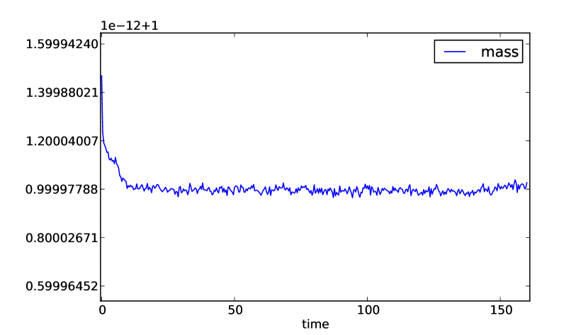
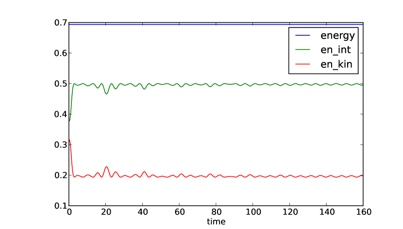
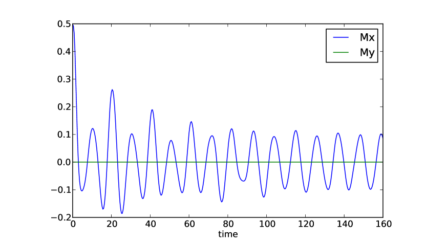
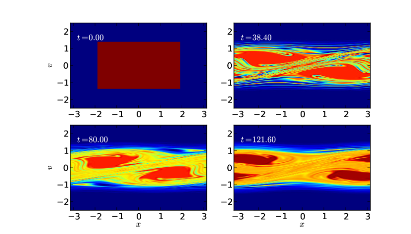
Figure 2: Simulations of the “HMF_in.resonances” example file. The mass evolution is zoomed to $1$ with a detail of $10^{-12}$. These figures are produced, with no modification, by the script “show_vmf90.py” that accompanies vmf90.

The figures generated by “show_vmf90.py” are reproduced in Fig. 2 without further processing. One can already observe the major features of the simulation: the normalization (“mass”, here) is respected to about $10^{-12}$ and the energy is conserved. The behavior of the magnetization, starting from $M_{x}=M_{0}=0.5$, is to decrease and then display sustained oscillations. Snapshots of the phase space are also displayed, at four regularly spaced times of the simulation, and the clustering behavior observed in Refs. [15, 5] is well reproduced.

5.1 Performing a parametric study

vmf90 comes with an example program, “parametric_run.py”, in the “scripts” directory to perform a parametric study of the HMF magnetization. Such a study represents a typical use of the program in the existing literature.

The example reproduces Fig. 3 of Ref. [11], albeit with a smaller number of grid points and a shorter sampling time, for a faster execution. The appearance of the figure is also changed to a scatter plot to make the implementation of the data collection more readable.

6 Simulations for the single-wave model

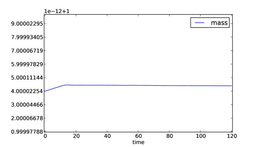
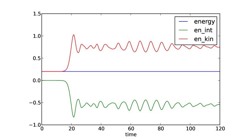
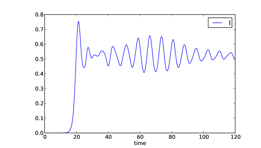
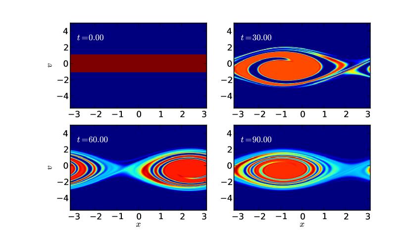
Figure 3: Simulations of the “FEL_in” example file. The mass evolution is zoomed to $1$ with a detail of $10^{-12}$. These figures are produced, with no modification, by the script “show_vmf90.py” that accompanies vmf90.

The single-wave model [16] represents an ensemble of particles in which the interaction is well represented by a single component of the electromagnetic field. In addition to the particles, represented by the distribution function $f$, one needs to consider also the field $A_{x}$, $A_{y}$ in the simulation as evidenced by the coupled evolution equations (10). As is typical, we track the evolution of the intensity of the field $I=\sqrt{A_{x}^{2}+A_{y}^{2}}$.

We consider a simulation that was presented in Ref. [6] with a homogeneous water bag initial condition of energy $U=0.2$ and a “seed” intensity given by $A_{x}=0.0001$, $A_{y}=0$. Without the seed, even unstable initial conditions may remain stuck because of the lack of granularity of the distribution. The panels of Fig. 3 are the direct output of the program “show_vmf90.py”. Mass conservation is respected with a relative accuracy of about $10^{-12}$, as it was for the HMF model. The other panels display the evolution of the energy and of the intensity of the wave. The snapshot displays the typical structure of a single “bump” in which the majority of the distribution function is found.

7 Discussion

We have presented an open-source implementation of the semi-Lagrangian algorithm for Vlasov simulations tailored for mean-field models. This code has served as the basis for several publications and its modular nature allows for an easy addition of other models. The Fortran code uses modern additions to the language that allows for structured programming. Other technical features include the use of HDF5 for the storage of simulation data, the inclusion of a simulation analysis program, revision control of the source code and an extensive in code documentation.

Appendix A Example configuration file

An example configuration file is provided, for the HMF model, in Fig. 4. This file is available as “HMF_in.stable_wb” in the program repository. Each parameter appears with an explicit denomination in the file.

model = HMF     ! the model name. is checked in the program
Nx = 256        ! number of points in x-direction
Nv = 512        ! number of points in v-direction
vmax = 2.5      ! size of the box
DT = 0.1        ! timestep
n_steps = 5     ! number of steps in inner loop
n_top = 300     ! number of executions for inner loop
n_images = 50   ! number of dumps of the phase space DF
IC = wb_eps     ! initial condition
width = 4.      ! \Delta\theta for initial condition
bag = 0.72      ! \Delta p for initial condition
epsilon = 0.001 ! initial perturbation of the profile
Nedf = 0        ! number of points for energy DF

Figure 4: Example configuration file “HMF_in”.

References

- [1] P.-H. Chavanis, Lynden-bell and tsallis distributions for the hmf model, Eur. Phys. J. B 53 (2006) 487. doi:10.1140/epjb/e2006-00405-5.
- [2] P.-H. Chavanis, Hamiltonian and brownian systems with long-range interactions: II. kinetic equations and stability analysis, Physica A 361 (2006) 81. doi:10.1016/j.physa.2005.06.088.
- [3] A. Campa, T. Dauxois, S. Ruffo, Statistical mechanics and dynamics of solvable models with long-range interactions, Phys. Rep. 480 (2009) 57. doi:10.1016/j.physrep.2009.07.001.
- [4] F. Bouchet, S. Gupta, D. Mukamel, Thermodynamics and dynamics of systems with long-range interactions, Physica A 389 (2010) 4389–4405. doi:10.1016/j.physa.2010.02.024.
- [5] A. Antoniazzi, F. Califano, D. Fanelli, S. Ruffo, Exploring the thermodynamic limit of hamiltonian models: Convergence to the vlasov equation, Phys. Rev. Lett. 98 (2007) 150602. doi:10.1103/PhysRevLett.98.150602.
- [6] P. de Buyl, D. Fanelli, R. Bachelard, G. D. Ninno, Out-of-equilibrium mean-field dynamics of a model for wave-particle interaction, Phys. Rev. ST Accel. Beams 12 (2009) 060704. doi:10.1103/PhysRevSTAB.12.060704.
- [7] P. de Buyl, Numerical resolution of the vlasov equation for the hamiltonian mean-field model, Commun. Nonlinear Sci. Numer. Simulat. 15 (2010) 2133–2139. doi:10.1016/j.cnsns.2009.08.020.
- [8] P. de Buyl, D. Mukamel, S. Ruffo, Self-consistent inhomogeneous steady states in hamiltonian mean-field dynamics, Phys. Rev. E 84 (2011) 061151. doi:10.1103/PhysRevE.84.061151.
- [9] P. de Buyl, D. Mukamel, S. Ruffo, Statistical mechanics of collisionless relaxation in a non-interacting system, Phil. Trans. R. Soc. A 369 (2011) 439–452. doi:10.1098/rsta.2010.0251.
- [10] P. de Buyl, P. Gaspard, Effectiveness of mixing in violent relaxation, Phys. Rev. E 84 (2011) 061139. doi:10.1103/PhysRevE.84.061139.
- [11] P. de Buyl, D. Fanelli, S. Ruffo, Phase transitions of quasistationary states in the hamiltonian mean field model, Central European Journal of Physics 10 (2012) 652–659. doi:10.2478/s11534-012-0010-6.
- [12] P. de Buyl, G. De Ninno, D. Fanelli, C. Nardini, A. Patelli, F. Piazza, Y. Y. Yamaguchi, Absence of thermalization for systems with long-range interactions coupled to a thermal bath, Phys. Rev. E 87 (2013) 042110. doi:10.1103/PhysRevE.87.042110.
- [13] S. Ogawa, Y. Y. Yamaguchi, Linear response theory in the vlasov equation for homogeneous and for inhomogeneous quasistationary states, Phys. Rev. E 85 (2012) 061115. doi:10.1103/PhysRevE.85.061115.
- [14] C. Z. Cheng, G. Knorr, The integration of the vlasov equation in configuration space, J. Comp. Phys. 22 (1976) 330. doi:10.1016/0021-9991(76)90053-X.
- [15] M. Antoni, S. Ruffo, Clustering and relaxation in hamiltonian long-range dynamics, Phys. Rev. E 52 (1995) 2361. doi:10.1103/PhysRevE.52.2361.
- [16] T. O’Neil, J. H. Winfrey, J. H. Malmberg, Nonlinear interaction of a small cold beam and a plasma, Phys. Fluids 14 (1971) 1204. doi:10.1063/1.1693587.
- [17] Y. Elskens, D. Escande, Microscopic Dynamics of Plasmas and Chaos, Institute of Physics Publishing, 2003.
- [18] R. Bachelard, T. Manos, P. de Buyl, F. Staniscia, F. S. Cataliotti, G. D. Ninno, D. Fanelli, N. Piovella, Experimental perspectives for systems based on long-range interactions, J. Stat. Mech. 2010 (2010) P06009. doi:10.1088/1742-5468/2010/06/P06009.
- [19] V. K. Decyk, C. D. Norton, B. K. Szymanski, How to support inheritance and run-time polymorphism in fortran 90, Comput. Phys. Commun. 115 (1998) 9. doi:10.1016/S0010-4655(98)00101-5.
- [20] V. K. Decyk, H. J. Gardner, Object-oriented design patterns in fortran 90/95: mazev1, mazev2 and mazev3, Comput. Phys. Commun. 178 (2008) 611. doi:10.1016/j.cpc.2007.11.013.
- [21] D. McCormack, Scientific Software Development in Fortran, Lulu.com, 2009.
-
[22]
L. Torvalds, Contributors.
[link].
http://git-scm.com/ -
[23]
D. van Heesch, Doxygen (1997).
http://www.stack.nl/~dimitri/doxygen/ -
[24]
P. de Buyl, P. Colberg, F. Höfling, H5MD :
HDF5 for molecular data.
http://nongnu.org/h5md/ - [25] P. de Buyl, P. H. Colberg, F. Höfling, H5md: A structured, efficient, and portable file format for molecular data, Comp. Phys. Commun.doi:10.1016/j.cpc.2014.01.018.
-
[26]
A. Collette, HDF5 for Python (2008).
http://h5py.alfven.org/ - [27] T. E. Oliphant, Python for scientific computing, Computing in Science & Engineering 9 (2007) 10–20. doi:10.1109/MCSE.2007.58.
-
[28]
J. D. Hunter, matplotlib (2002).
http://matplotlib.org/ -
[29]
A. Vaught, P. Brook, Gnu fortran (2002).
http://gcc.gnu.org/fortran/ - [30] E. Sonnendrucker, J. Roche, P. Bertrand, A. Ghizzo, The semi-lagrangian method for the numerical resolution of the vlasov equation, J. Comp. Phys. 149 (1999) 201. doi:10.1006/jcph.1998.6148.