On long-term boundedness of Galerkin models

Abstract

We investigate linear-quadratic dynamical systems with energy preserving quadratic terms. These systems arise for instance as Galerkin systems of incompressible flows. A criterion is presented to ensure long-term boundedness of the system dynamics. If the criterion is violated, a globally stable attractor cannot exist for an effective nonlinearity. Thus, the criterion represents a minimum requirement for a physically justified Galerkin model of viscous fluid flows. The criterion is exemplified e.g. for Galerkin systems of two-dimensional cylinder wake flow models in the transient and the post-transient regime, the Lorenz system, and for physical design of a Trefethen-Reddy Galerkin system. There are numerous potential applications of the criterion, for instance system reduction and control of strongly nonlinear dynamical systems.

1 Introduction

Focus of this paper is the a priori characterisation of the long-term behaviour of a linear-quadratic differential equation system with energy preserving quadratic term. Such a dynamical system can be obtained by the spectral discretisation of the Navier-Stokes equation. More generally, many traditional Galerkin models with orthonormal basis functions fall in this category (Fletcher, 1984). Of particular interest is the long-term behaviour and attractor properties which can be ideally extracted analytically from the dynamical system. For instance, a meaningful model can be requested to have globally bounded solutions. Respective analytical methods for linear-quadratic Galerkin systems are still in their infancy. For a variety of related problems, e.g., properties of fixed points, efficient tools for dynamical system analyses (see, e.g., Guckenheimer & Holmes, 1986; Khalil, 2002) and tensor structure analyses have been well elaborated (see, e.g., Kolda & Bader, 2009).

In this study, focus will be placed on low-order Galerkin models of the coherent flow dynamics as a simple starting point. These models are of particular interest for the understanding of the nonlinear dynamics (see, e.g., Holmes et al. , 2012) and are key enablers of closed-loop flow control applications (see, e.g., Noack et al. , 2011). Examples of low-order models include boundary layers (Rempfer & Fasel, 1994), cylinder wakes (Deane et al. , 1991; Noack et al. , 2003), mixing layers (Noack et al. , 2005; Wei & Rowley, 2009), lid-driven cavities (Cazemier et al. , 1998; Balajewicz et al. , 2013), and supersonic diffuser flows (Willcox & Megretski, 2005). However, these models tend to be fragile: Small changes of system parameters may give rise to unphysical divergent solutions, at least for a subset of initial conditions. Thus, parameter identification is a delicate task and a priori knowledge about the long-term behaviour of Galerkin models for all initial conditions is highly desirable.

For a priori analyses of the long-term behaviour, the optimum is represented by analytical solutions. However, the general analytical solution of a class of linear-quadratic differential equation systems, including, e.g., the Lorenz system, appears to be unrealisable within the frame of the current state of the art. In contrast, the simple analytical structure of a linear-quadratic Galerkin system provides a key enabler for the application of a rich kaleidoscope of the methodologies provided by the theory of nonlinear dynamics and control theory. One example is given by the utilisation of Lyapunov’s direct method (Lyapunov, 1892). In fluid mechanics this method is adopted mainly for two purposes. Firstly, it is employed for nonlinear stability analyses of fixed points and for model-based flow control design. The methodology is well-established for linear systems (see, e.g., Kim & Bewley, 2007; Sipp et al. , 2010), and generalised for nonlinear systems (see, e.g., Aamo & Krstić, 2002; Khalil, 2002). Applications for Lyapunov-based flow control design are demonstrated in numerical and experimental investigations (see, e.g., Gerhard et al. , 2003; Samimy et al. , 2007; Schlegel et al. , 2009, 2012). A second purpose of the direct Lyapunov method is to ensure hydrodynamic stability via the sufficient condition for a monotonically decreasing fluctuation energy (see, e.g., Joseph, 1976; Drazin & Reid, 1981). This leads to the identification of lower bounds for the critical Reynolds number of laminar-turbulent transition and the identification of flow structures of maximal energy growth.

However, the application range of Lyapunov’s direct method is restricted by the lack of a systematic approach for the construction of appropriate Lyapunov functions. The usage of conventional Lyapunov functions like the total kinetic energy might fail the desired purpose, e.g. to show stability for interior flows: The linear stability matrix is far from being normal over a large range of Reynolds numbers. Temporal energy growth is observed which is traced back to interactions of non-orthogonal eigenvectors (Trefethen et al. , 1993; Schmid & Henningson, 2001). The application range of Lyapunov’s direct method is enhanced for some configurations (Galdi & Padula, 1990; Straughan, 2004). However, the identification of strict lower bounds of flow stability is often far below the critical Reynolds number.

The difficulty of finding an appropriate Lyapunov function can partially be ascribed by the design goal, e.g. by ensuring the global stability of fixed points in the whole phase space. Instead, conditions for the existence of an arbitrary globally attractive solution are considered. In this paper, we focus on the existence of trapping regions employing Lyapunov’s direct method (Swinnerton-Dyer, 2000). Coarsely stated, a trapping region is a domain in state space such that each trajectory once entered the trapping region will remain inside the trapping region for all times (Meiss, 2007). In case of a (globally) attracting trapping region, all trajectories outside of the trapping region converge to the trapping region. The assumption of the existence of an attracting trapping region is connected with several other properties of dynamical systems (see figure 1). In case that an attracting trapping regions exists, the system dynamics is long-term bounded because the habitat of the long-term dynamics is represented by this trapping region. An existing (globally stable) single or multiple attractor must be embedded inside of an attracting trapping region.

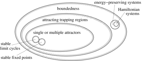
Figure 1: Venn diagram of dynamical systems.

The existence of an attracting trapping region can be ensured via the existence of a function which is strictly of Lyapunov function type outside of a trapping region. As a well-known example, the existence of an attracting trapping region is shown for the Lorenz system (Swinnerton-Dyer, 2001). We follow this hint to investigate long-term boundedness and to estimate the extent of existing attractors. In particular, we focus on the generality for the considered class of linear-quadratic dynamical systems and the simplicity of the construction of the respective Lyapunov functions.

The content of this paper is structured as following: In section 2, the class of the considered dynamical systems is defined. In section 3, Lyapunov’s direct method is generalised for the identification of trapping regions. A criterion for long-term boundedness and existence of globally stable attractors is proposed in section 4 and its range of validity is identified. Analytical and numerical application results are demonstrated for the investigation of long-term boundedness of Galerkin systems for the post-transient and transient dynamics of a two-dimensional cylinder wake flow in section 5. Moreover, a Galerkin system featuring nonlinear characteristics of the Trefethen-Reddy system is identified in section 6. The Lorenz system is investigated in section 7. In the first appendix section A, the generality of flow configurations is demonstrated, for which the Galerkin method extracts dynamical systems of the considered class. In section 8, the main findings are summarised and future directions are indicated.

2 Galerkin models of fluid flows

In this section, the considered class of dynamical systems is introduced. These systems naturally arise as Galerkin models of the incompressible Navier-Stokes equation in a steady domain $\Omega$ with stationary boundary conditions (see, e.g. Holmes et al. , 2012). Galerkin models are typically extracted in two steps. First, a finite-dimensional Hilbert function subspace ${\mathcal{H}}$ is chosen. This subspace is spanned by space dependent modes ${\boldsymbol{u}}_{i}$, $i=1\ldots N$, which form an orthonormal basis in this Hilbert space. The flow ${\boldsymbol{u}}$ is modelled by a Galerkin approximation with a base flow ${\boldsymbol{u}}_{0}$ and an expansion for the fluctuation ${\boldsymbol{u}}^{\prime}={\boldsymbol{u}}-{\boldsymbol{u}}_{0}$:

$${\boldsymbol{u}}({\boldsymbol{\xi}},t) = {\boldsymbol{u}}_{0}({\boldsymbol{\xi}})\,+\,\sum_{i=1}^{N}x_{i}(t)\,{\boldsymbol{u}}_{i}({\boldsymbol{\xi}}).$$ (1)

The flow state is described by the time-dependent modal amplitudes $x_{i}$. The spatial variables are denoted by ${\boldsymbol{\xi}}$ and the time by $t$. The base flow ${\boldsymbol{u}}_{0}$ might represent a steady Navier-Stokes solution or mean flow. The main purpose for the introduction of the base flow is that (1) satisfies the boundary conditions for arbitrary choices of modal coefficients $x_{i}$ (Ladyz̆henskaya, 1963). The expansion modes ${\boldsymbol{u}}_{i}$, $i=1,\ldots,N$, may arise from a proper orthogonal decomposition of snapshot data or from other mathematical considerations Noack & Eckelmann (1994).

In the second step, a dynamical system is identified. At first, the Navier-Stokes equation is projected onto the Hilbert subspace ${\mathcal{H}}$ (see, e.g. Noack et al. , 2011). As result of the modelling process, a class of dynamical systems is considered, formulated in the vector space of the state variable ${\boldsymbol{x}}=[x_{1},\ldots,x_{N}]^{\top}$ by

$$\frac{dx_{i}}{dt} = c_{i}+\sum\limits_{j=1}^{N}l_{ij}\,x_{j}+\sum\limits_{j,k=1}^{N}q_{ijk}\,x_{j}\,x_{k}$$ (2)

with the real numbers $c_{i}$, $l_{ij}$, $q_{ijk}$, for $i,j,k=1,\ldots,N$. Without loss of generality, the $q_{ijk}$’s are assumed to be symmetric in the last two indices, i.e.

$$q_{ijk}=q_{ikj}, i,j,k=1,\ldots,N.$$ (3)

The quadratic term of (2) can be shown to be energy-preserving for a large class of boundary conditions (see appendix section A). This means that the sums of the quadratic coefficients over index permutations are zero

$$q_{ijk}+q_{ikj}+q_{jik}+q_{jki}+q_{kij}+q_{kji} = 2\,q_{ijk}+2\,q_{jik}+2\,q_{kij}\;=\;0\,,$$

$$i,j,k = 1,\ldots,N\,.$$ (4)

This property is postulated for the class of dynamical systems discussed in this paper.

The energy-preserving quadratic term has an important effect on the evolution of the fluctuation energy

$$K := \frac{1}{2}\sum_{i=1}^{N}x_{i}^{2}\geq 0.$$ (5)

If ${\boldsymbol{u}}_{0}$ is the mean flow, then $K$ denotes the standard turbulent kinetic energy (TKE) of statistical fluid mechanics. The time derivative of $K$ reads

$$\frac{dK}{dt}\;=\;[\boldsymbol{\nabla}_{\boldsymbol{x}}K]^{\top}\,\frac{d{\boldsymbol{x}}}{dt}\;=\;\sum_{i=1}^{N}x_{i}\,f_{i}({\boldsymbol{x}})\;=\;\sum\limits_{i=1}^{N}c_{i}\,x_{i}\;+\sum\limits_{i,j=1}^{N}l_{ij}\,x_{i}\,x_{j},$$ (6)

i.e. the quadratic terms cancel each other out by (4).

Defining the vector ${\boldsymbol{c}}:=\left[c_{1},\ldots,c_{N}\right]^{\top}$ and matrix ${\mathsfbi{L}}:=\left[l_{ij}\right]_{i,j=1}^{N}$, the evolution of $K$ is given in a simple vector-matrix notation via

$$\frac{dK}{dt}\;=\;{\boldsymbol{c}}^{\top}{\boldsymbol{x}}\;+\;{\boldsymbol{x}}^{\top}\mathsfbi{L}_{S}\,{\boldsymbol{x}}\,,$$ (7)

where the symmetric part $\mathsfbi{L}_{S}:=\,\left({\mathsfbi{L}}+{\mathsfbi{L}}^{\top}\right)/2$ of ${\mathsfbi{L}}$ is introduced.

3 A generalisation of Lyapunov’s direct method

The purpose of this section is twofold. First, a generalised Lyapunov’s direct method is used to guarantee long-term boundedness of a example dynamical system without the existence of a globally stable fixed point. Second, an amplitude limiting mechanism of nonlinear dynamical systems is elaborated qualitatively and quantitatively, requiring the introduction of ’monotonically attracting trapping regions’. The long-term behaviour is characterised by the evolution of the energy of the system state with respect to the origin. For mathematical convenience and physical intuition, the energy $K$ defined in (5) is chosen. This is modulo factor $1/2$ the square of the Euclidean distance to the origin given by the Euclidean norm $\|.\|=\sqrt{2\,K(.)}$.

3.1 Long-term boundedness of an example system

As a first example of an energy limiting mechanism, the two-dimensional system

$$\frac{dx_{1}}{dt} = -x_{1}\;+\;x_{2}^{2}\,,$$ (8a)

$$\frac{dx_{2}}{dt} = x_{2}\;-\;x_{1}\,x_{2}\,,$$ (8b)

is considered. By the linear, symmetric part ${\mathsfbi{L}}_{S}={\mathsfbi{L}}=\left[\begin{array}[]{cc}-1&0\\ 0&1\end{array}\right]$ of the two-dimensional system, the direction $[0,1]^{\top}$ with positive energy growth and the direction $[1,0]^{\top}$ with negative energy growth are obtained (see figure 2). The field of the quadratic term deflects the trajectories from directions of growing energy into the directions of shrinking energy. In result of the interaction of the linear and the quadratic term, all trajectories are attracted by one of the stable fixed points $[1,1]^{\top}$, $[1,-1]^{\top}$, or along the abscissa to the origin which represents an unstable fixed point.

+           =     

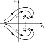
Figure 2: Fields of the linear term (left), the quadratic term (middle), and stable fixed point behaviour (right) of system (8).

There is no quadratic Lyapunov function by which the convergence to one of the stable fixed points can be proven a priori. The Lyapunov function does not even exist in the corresponding open half-planes of attraction. The energy is increasing or decreasing in dependence of the location of the state. There are phase-space areas of positive or negative energy growth. If the dynamics along the trajectory is dominated by negative energy growth, the system state is attracted e.g. to fixed points like in system (8). If the dynamics is dominated by positive energy growth, the trajectories may diverge to infinity.

By the transformation

$${\boldsymbol{y}} = {\boldsymbol{x}}-{\boldsymbol{m}}$$ (9)

an arbitrary state ${\boldsymbol{m}}=[m_{1},\ldots,m_{N}]^{\top}$ can be shifted into the origin of ${\boldsymbol{y}}$. The fluctuation energy with respect to $\boldsymbol{m}$ is defined by

$$K_{\boldsymbol{m}} := \sum_{i=1}^{N}y_{i}^{2}\;=\;\sum_{i=1}^{N}(x_{i}-m_{i})^{2}\,.$$ (10)

Its evolution is given by

$$\frac{d}{dt}K_{\boldsymbol{m}} = {\boldsymbol{y}}^{\top}{\mathsfbi{A}}_{S}\,{\boldsymbol{y}}+{\boldsymbol{d}}^{\top}{\boldsymbol{y}}\;=\;\left({\boldsymbol{x}}-{\boldsymbol{m}}\right)^{\top}{\mathsfbi{A}}_{S}\left({\boldsymbol{x}}-{\boldsymbol{m}}\right)+{\boldsymbol{d}}^{\top}\left({\boldsymbol{x}}-{\boldsymbol{m}}\right)\,,$$ (11)

where ${\boldsymbol{d}}$ and ${\mathsfbi{A}}_{S}$ denote the constant and linear symmetric part of the transformed Galerkin system.

Employing ${\boldsymbol{m}}=[2,0]^{\top}$, the example system (8) is given for the shifted coordinates by

$$\frac{dy_{1}}{dt} = -2\;-\;y_{1}\;+\;y_{2}^{2}\,,$$ (12a)

$$\frac{dy_{2}}{dt} = -y_{2}\;-\;y_{1}\,y_{2}\,,$$ (12b)

leading to the power balance with respect to the new origin,

$$\frac{d}{dt}K_{\boldsymbol{m}} = -2\,y_{1}\;-\;y_{1}^{2}-y_{2}^{2}\,.$$ (13)

Hence, the energy is growing only in a bounded domain defined by the interior of the circle given by $(y_{1}+1)^{2}+y_{2}^{2}<1$. If $K_{\boldsymbol{m}}$ is large, it will decrease and the trajectories cannot escape each circle $B$ with the origin at the centre in which the bounded domain of energy growth is contained. In conclusion, the long-term dynamics of the shifted system and consequently of the system (8) are bounded! Outside of each $B$, the energy $K_{\boldsymbol{m}}$ represents a strict Lyapunov function and thus Lyapunov’s direct method is effective. Inside of $B$, the energy $K_{\boldsymbol{m}}$ can grow and thus Lyapunov’s direct method cannot be applied.

3.2 Monotonically attracting trapping regions

For a generalisation of this approach, we introduce monotonically attracting trapping regions. A trapping region $D\subseteq\mathbb{R}^{N}$ is a compact set, in which each trajectory remains once it has entered, i.e. from ${\boldsymbol{x}}(s)\in D$ it follows that ${\boldsymbol{x}}(t)\in D$ for all $t>s$. A trapping region is termed (globally) monotonically attracting, if an energy is strictly monotonically decreasing along all trajectories starting from an arbitrary state outside of $D$. This implies that outside of the trapping region the energy possesses the mathematical properties of a strict Lyapunov function. For our choice of energy $K_{\boldsymbol{m}}=\|{\boldsymbol{x}}-{\boldsymbol{m}}\|^{2}/2$, it is sufficient to consider closed balls

$$B({\boldsymbol{m}},R) := \left\{{\boldsymbol{x}}\in\mathbb{R}^{N}\,:\,\|{\boldsymbol{x}}-{\boldsymbol{m}}\|^{2}\leq R^{2}\right\}$$ (14)

with the centre ${\boldsymbol{m}}$ and radius $0<R<\infty$. For later reference, these closed balls are also expressed in terms of translated coordinates $\boldsymbol{y}=\boldsymbol{x}-\boldsymbol{m}$:

$$B_{\boldsymbol{y}}(R) := \left\{{\boldsymbol{y}}\in\mathbb{R}^{N}\,:\,\|{\boldsymbol{y}}\|\leq R^{2}\right\}.$$ (15)

Here, each closed ball containing $D$ as a subset is a monotonically attracting trapping region as well.

If all eigenvalues of ${\mathsfbi{A}}_{S}$ are negative, i.e. $0>\lambda_{1}\geq\ldots\geq\lambda_{N}$, then Lyapunov’s direct method is effective for large deviations. This is immediately shown by the energy evolution equation (11). In the following, the energy evolution equation is analysed to obtain monotonically attracting trapping regions.

For that, a negative definite linear symmetric part ${\mathsfbi{A}}_{S}$ is postulated in the following. Invoking the diagonalisation

$$\mathsfbi{A}_{S}\;=\;{\mathsfbi{T}}^{\top}\,{\mathsfbi{\Lambda}}\,{\mathsfbi{T}}$$ (16)

of the symmetric matrix ${\mathsfbi{A}}_{S}$ with the diagonal eigenvalue matrix ${\mathsfbi{\Lambda}}$ and the orthogonal matrix ${\mathsfbi{T}}$ comprising the eigenvectors, a transformation

$${\boldsymbol{z}} = {\mathsfbi{T}}\,{\boldsymbol{y}}$$ (17)

is defined, preserving the energy $K_{\boldsymbol{m}}$. Employing this coordinate transformation (rotation + reflections), the energy growth is given by

$$\frac{d}{dt}K_{\boldsymbol{m}}\;=\;\sum\limits_{i=1}^{N}h_{i}\,z_{i}\,+\,\lambda_{i}\,z_{i}^{2}\;=\;\sum\limits_{i=1}^{N}\lambda_{i}\,\left(z_{i}+\,\frac{h_{i}}{2}\right)^{2}\,-\,\sum\limits_{i=1}^{N}\lambda_{i}\frac{h_{i}^{2}}{4}\,.$$ (18)

with the components $h_{i}$ of ${\boldsymbol{h}}\,:=\,{\boldsymbol{d}}\,{\mathsfbi{T}}^{\top}$.

For ${\boldsymbol{d}}={\boldsymbol{0}}$ and hence ${\boldsymbol{h}}={\boldsymbol{0}}$, the energy is a strict Lyapunov function since $\lambda_{i}<0$, $i=1,\ldots,N$, has been assumed. In addition, a globally stable fixed point is situated at the origin. For ${\boldsymbol{d}}\neq{\boldsymbol{0}}$ and hence ${\boldsymbol{h}}\neq{\boldsymbol{0}}$, the energy growth can be positive close to the origin. In more detail, the sign of the energy growth is changing at the boundary of an ellipsoid $E$ which is defined via

$$\sum\limits_{i=1}^{N}\frac{1}{\alpha_{i}^{2}}\left(z_{i}+\,\frac{h_{i}}{2}\right)^{2}\;=\;1 \alpha_{i}\;:=\;\sqrt{\frac{\sum_{j=1}^{N}\lambda_{j}\,h_{j}^{2}}{4\,\lambda_{i}}}\,.$$ with (19)

In the interior of the ellipsoid $E$, the energy growth is positive with a maximum growth at the centre $-{\boldsymbol{h}}/2$. Outside of the ellipsoid the energy is decreasing. At the boundary, the energy stays constant. Note, that the origin is situated at the boundary of the ellipsoid because it is trivially solving equation (19). The half-axes $\alpha_{i}$ are directly proportional to the Euclidean norm of ${\boldsymbol{h}}$ and hence of ${\boldsymbol{d}}$.

After a finite time, the system state is trapped in the smallest closed ball $B$ with centre at the origin of the ${\boldsymbol{y}}$-coordinates such that the ellipsoid $E$ is contained. Hence, the smallest monotonically attracting trapping ball is given by $B$!

The long-term behaviour of the system, represented e.g. by an globally stable attractor, is either part of the boundary without growth of $K_{\boldsymbol{m}}$, or is alternating between positive energy growth inside of $E$ and negative energy growth in $B\setminus E$ (see figure 3). The case ${\boldsymbol{d}}={\boldsymbol{0}}$ can be seen as a degeneration of $E$ and $B$ to the fixed point at the origin.

Figure 3: Principal sketch of boundedness of a solution of a Galerkin system (2) in a closed ball $B$. For simplicity, the origin is not shifted, i.e. ${\boldsymbol{m}}={\boldsymbol{0}}$. The growth of energy to the origin is positive only inside of an ellipsoid $E$.

4 A sufficient criterion for long-term boundedness

In this section, a sufficient criterion for long-term boundedness of Galerkin systems is derived to exclude infinite blow ups of the system state ${\boldsymbol{x}}(t)$ in finite or infinite periods of time. Via the criterion of theorem 1 below, the existence of monotonically attracting trapping regions is considered. For the generic class of Galerkin systems (2) with effective nonlinearity, it is shown that a globally stable attractor can only exist if there is a monotonically attracting trapping region. The results of this section will culminate in the procedure sketched in figure 4, guiding the determination of the long-term behaviour of the Galerkin systems (2).

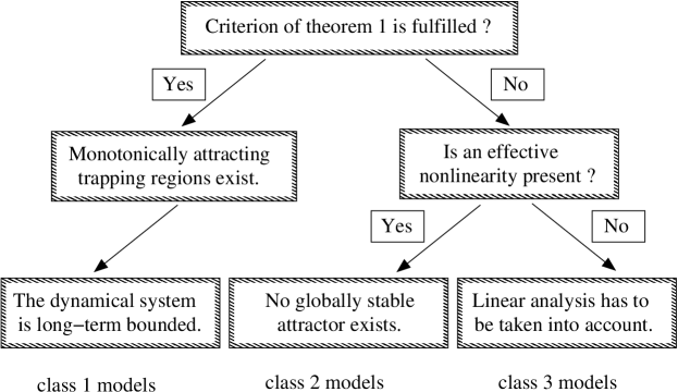
Figure 4: Decision tree diagram for long-term boundedness of linear-quadratic systems.

To keep the notation simple, the following vector-matrix representation of (2) is employed using the symmetric matrices ${\mathsfbi{Q}^{(\alpha)}}:=\left[q_{\alpha ij}\right]_{i,j=1}^{N}$, $\alpha=1,\ldots,N$,

$$\frac{d{\boldsymbol{x}}}{dt} = {\boldsymbol{c}}+{\mathsfbi{L}}\,{\boldsymbol{x}}+\left[\,{\boldsymbol{x}}^{\top}\,{\mathsfbi{Q}}^{(1)}\,{\boldsymbol{x}}\,,\ldots,\,{\boldsymbol{x}}^{\top}\,{\mathsfbi{Q}}^{(N)}\,{\boldsymbol{x}}\,\right]^{\top}.$$ (20)

Using this nomenclature, the condition (4) can be rewritten as

$$q^{(i)}_{jk}+q^{(j)}_{ik}+q^{(k)}_{ij}=0, i,j,k=1,\ldots,N$$ (21)

employing the elements $q^{(i)}_{jk}$, $j,k=1,\ldots,N$ of the symmetric matrices ${\mathsfbi{Q}}^{(i)}$.

For the translated variable $\boldsymbol{y}=\boldsymbol{x}-\boldsymbol{m}$, the dynamical system

$$\frac{d{\boldsymbol{y}}}{dt} = {\boldsymbol{d}}+{\mathsfbi{A}}\,{\boldsymbol{y}}+\left[\,{\boldsymbol{y}}^{\top}\,{\mathsfbi{Q}}^{(1)}\,{\boldsymbol{y}}\,,\ldots,\,{\boldsymbol{y}}^{\top}\,{\mathsfbi{Q}}^{(N)}\,{\boldsymbol{y}}\,\right]^{\top}$$ (22)

with

$${\boldsymbol{d}}:=\left(c_{i}+\sum_{j=1}^{N}l_{ij}m_{j}+\sum_{j,k=1}^{N}q_{ijk}m_{j}m_{k}\right)_{i=1}^{N}$$ (23)

and

$${\mathsfbi{A}}:=\left(l_{ij}+\sum_{k=1}^{N}(q_{ijk}+q_{ikj})\,m_{k}\right)$$ (24)

is obtained. Note that the symmetric part $\mathsfbi{A}_{S}$ of ${\mathsfbi{A}}$ can be represented as a linear combination of the symmetric part $\mathsfbi{L}_{S}$ of ${\mathsfbi{L}}$ and of the ${\mathsfbi{Q}}^{(i)}$’s

$$\mathsfbi{A}_{S}\;:=\;\frac{1}{2}\left({\mathsfbi{A}}+{\mathsfbi{A}}^{\top}\right) = \mathsfbi{L}_{S}\;-\;\sum\limits_{i=1}^{N}\,{m_{i}}\;{\mathsfbi{Q}}^{(i)}\,,$$ (25)

exploiting the symmetry properties (4) and (3).

Employing the translation, a simple condition for the existence of a monotonically attracting trapping region can be found. If all eigenvalues of ${\mathsfbi{A}}_{S}$ are negative, i.e. $0>\lambda_{1}\geq\ldots\geq\lambda_{N}$, then the energy evolution equation is transformed to equation (18) employing the rotation of the coordinate system to the principal axes. Hence, the domain of energy growth is identified to be inside of the ellipsoid given by (19). Every ball with the origin ${\boldsymbol{y}}={\boldsymbol{0}}$ at the centre, which contains the ellipsoid, is a monotonically attracting trapping region. Consider the estimate

$$\alpha_{i} \leq \sqrt{\frac{\lambda_{N}}{4\lambda_{1}}}\,\|{\boldsymbol{d}}\|\,,$$ (26)

invoking the definition (19) of the half-axes $\alpha_{i}$. Then a radius of such a ball, not necessarily the infinimum amongst such radii, is given by $R_{m}=\sqrt{\lambda_{N}/\lambda_{1}}\|{\boldsymbol{d}}\|$.

On the other hand, given a monotonically attracting trapping region, the distance of every state ${\boldsymbol{x}}$ outside the trapping region to a state ${\boldsymbol{m}}$ inside of the trapping region is monotonically decreasing by definition. This is only true if the right-hand side of the power balance (11) is negative for an ${\boldsymbol{m}}$ inside the trapping region and if the energy $K_{\boldsymbol{m}}$ is large enough. By symmetry considerations this requires that all eigenvalues of ${\mathsfbi{A}}_{S}$ are negative.

The above-mentioned results are summarised in the following theorem

Theorem 1

MONOTONICALLY ATTRACTING TRAPPING REGIONS
Regarding the system (20), the following two statements are equivalent:

1. There is a monotonically attracting trapping region.

2. There is an ${\boldsymbol{m}}$, such that there are only negative eigenvalues $0>\lambda_{1}\geq\ldots\geq\lambda_{N}$ of the symmetric linear part ${\mathsfbi{A}}_{S}$ (25) of the shift-transformed system (22).

If these conditions are true, $R_{m}=\sqrt{\lambda_{N}/\lambda_{1}}\>\|{\boldsymbol{d}}\|$ is a radius such that $B({\boldsymbol{m}},R_{m})$ is a monotonically attracting trapping region.

In conclusion, a sufficient condition for the long-term boundedness of systems (20) over an infinite time horizon has been found.

As a first example of an application of the criterion, we show the existence of a monotonically attracting trapping region for the system (8). It can be written in the form of equation (20) with

$${\boldsymbol{c}}=\left[\begin{array}[]{c}0\\ 0\end{array}\right],\;{\mathsfbi{L}}\;=\;\left[\begin{array}[]{cc}-1&0\\ 0&1\end{array}\right],\;{\mathsfbi{Q}^{(1)}}\;=\;\left[\begin{array}[]{cc}0&0\\ 0&1\end{array}\right],\;{\mathsfbi{Q}^{(2)}}\;=\;\left[\begin{array}[]{cc}0&-\frac{1}{2}\\ -\frac{1}{2}&0\end{array}\right].$$ (35)

Considering the translation with ${\boldsymbol{m}}=[2,0]^{\top}$, and invoking (25), the symmetric part of the transformed system is

$${\mathsfbi{A}}_{S} = \left[\begin{array}[]{cc}-1&0\\ 0&-1\end{array}\right].$$ (38)

By the negative definiteness of ${\mathsfbi{A}}_{S}$, the existence of a monotonically attracting trapping region is shown. One of these regions is given by the closed ball $B_{\boldsymbol{y}}(2)$ in the ${\boldsymbol{y}}$-coordinates (see (15)) and equivalently by $B({\boldsymbol{m}},2)$ in the ${\boldsymbol{x}}$-coordinates (see (14)). All solutions, given by the stable and unstable fixed points are situated inside of $B$ and at the boundary of the ellipsoid $E$ defined by equation (19), along which the energy $K_{\boldsymbol{m}}$ is maintained.

Although boundedness of a large class of systems is ensured, there might exist long-term bounded systems even with a globally stable fixed point which do not fit the condition of theorem 1. One class is given by Hamiltonian systems in which the energy $K_{\boldsymbol{m}}$ is preserved. Here, ${\mathsfbi{A}}_{S}={\mathsfbi{0}}$, because the distance to an ${\boldsymbol{m}}$ of the initial values remains constant for all times. All trajectories are embedded in invariant spaces, representing shells of constant distance around the centre. Hence the dynamics are bounded, but globally stable trapping regions or even a globally stable attractor do not exist.

Another class is given from the linear system behaviour of (20) with vanishing nonlinear term ${\mathsfbi{Q}}^{(i)}={\mathsfbi{0}}$, $i=1,\ldots,N$, ${\boldsymbol{c}}={\boldsymbol{0}}$, and a non-normal matrix ${\mathsfbi{L}}$. Here, an attracting behaviour can be accompanied with temporal energy growth as known from the theory of non-normal matrices (Trefethen & Embree, 2005). Even if there is a globally stable fixed point, the convergence of the trajectories can be non-monotonous with alternating increase and decrease of the distance to the fixed point.

However in the generic case of an effective nonlinearity, each globally non-monotonically attracting set is embedded in a larger monotonically attracting trapping region. To introduce the notion of an effective nonlinearity, a reformulation of the transformed system (22) is considered. Let ${r}:=\|{\boldsymbol{y}}\|>0$ be the amplitude (radius) of the state and ${\boldsymbol{w}}:={\boldsymbol{y}}/{r}$ the ‘generalised phase’ (direction) on the unit ball $\partial B_{\boldsymbol{y}}(1)$. It yields

$$\frac{d{\boldsymbol{w}}}{dt} = \frac{1}{r}{\boldsymbol{d}}+{\mathsfbi{A}}\,{\boldsymbol{w}}+{r}\,\left[\,{\boldsymbol{w}}^{\top}\,{\mathsfbi{Q}}^{(1)}\,{\boldsymbol{w}}\,,\ldots,\,{\boldsymbol{w}}^{\top}\,{\mathsfbi{Q}}^{(N)}\,{\boldsymbol{w}}\,\right]^{\top}\,,$$ (39a)

$$\frac{d{r}}{dt} = {\boldsymbol{d}}^{\top}{\boldsymbol{w}}+{r}\;{\boldsymbol{w}}^{\top}\mathsfbi{A}_{S}\,{\boldsymbol{w}}\,.$$ (39b)

The focus of interest is on large distances $r$ from the origin ${\boldsymbol{m}}$. The nonlinearity is termed effective if the constant and linear term of the phase equation (39a) can be neglected for large $r$

$$\frac{d{\boldsymbol{w}}}{dt} = {r}\,\left[\,{\boldsymbol{w}}^{\top}\,{\mathsfbi{Q}}^{(1)}\,{\boldsymbol{w}}\,,\ldots,\,{\boldsymbol{w}}^{\top}\,{\mathsfbi{Q}}^{(N)}\,{\boldsymbol{w}}\,\right]^{\top}\,,$$ (40)

i.e. the trajectories are driven by the dynamics of the equations (40) and (39b). Generically, the spatial asymptotical behaviour of the considered Galerkin systems (2) is described by these two equations. However, this is not true if there exist invariant manifolds of (20) with vanishing quadratic term, i.e. ${\boldsymbol{x}}^{\top}{\mathsfbi{Q}}^{(i)}{\boldsymbol{x}}={\boldsymbol{0}}$ for all corresponding states. Here, linear analyses have to be applied in addition to identify the long-term behaviour conclusively. For illustration, a corresponding example is detailed in subsection B.2 of the appendix section B.

For effective nonlinearity, the dynamics of large deviations is independent from the antisymmetric part of the linear term: the dynamics of the phase ${\boldsymbol{w}}$ is determined solely by the quadratic term, the dynamics of $r$ solely by the symmetric part of the linear term and the constant term. The mechanisms for temporal energy growth resulting from non-orthogonal eigendirections of non-normal matrices are excluded for large $r$. It can be concluded for each attracting trapping region, that it is embedded in a monotonically attracting trapping region.

These results are summarised in the following theorem.

Theorem 2

TRAPPING REGIONS
Consider a system (20) with effective nonlinearity, i.e. the dynamics of large deviations of the shifted system (22) can be described by (39b) and (40). Then each (globally) attracting trapping region is contained in a monotonically attracting trapping region. In particular, the existence of a monotonically attracting trapping region is necessary for the existence of a globally stable attractor.

In conclusion, the long-term behaviour is determined via application of the procedure illustrated in figure 4. For the criterion of theorem 1, $N$ components of ${\boldsymbol{m}}$ have to be found such that the $N$ eigenvalues of ${\mathsfbi{A}}_{S}$ given by (25) are negative. While this can be analytically done for systems of dimension lower than or equal to four, for larger dimensions numerical linear algebra and multidimensional optimisation like simulated annealing has to be employed.

5 Long-term boundedness of Galerkin models for cylinder wake flows

In this section, we investigate the long-term boundedness of a hierarchy of Galerkin models for periodic cylinder wakes (Noack et al. , 2003). The considered systems include a 3-dimensional mean-field system (subsection 5.1), an 8-dimensional POD model (subsection 5.2) and a 9-dimensional generalisation of this POD model with a stabilising shift mode (subsection 5.3). The existence of a monotonically attracting trapping region is demonstrated analytically for the mean-field system which is known to have a globally stable limit cycle. The corresponding existence is also numerically shown for the 9-dimensional model which generalises the mean-field system by inclusion of the 2nd to 4th harmonics. The existence of a monotonically attracting trapping region is disproved for the 8-dimensional system which has a locally stable limit cycle but also solutions converging to infinity. Thus, the theorems of section 4 proof numerically suggested behaviour of the hierarchy of Galerkin models.

5.1 On the long-term boundedness of a mean-field system

We consider a mean-field system for a soft onset of oscillatory fluctuations (Noack et al. , 2003) in fluid flows. The state contains 3 coordinates: $x_{1}$ and $x_{2}$ describe the amplitude of the phase of the oscillatory fluctuation and $x_{3}$ characterises the mean-field deformation. The origin $x_{1}=x_{2}=x_{3}=0$ corresponds to the steady solution. For simplicity, many parameters of the general mean-field model (see, e.g., Noack et al. , 2011) are set to zero or unity, following Sec. 2.1 of Noack et al.  (2003). Only the bifurcation parameter $\mu$ is left. The resulting mean-field system reads

$$\frac{dx_{1}}{dt} = \mu\,x_{1}\;-\;x_{2}\;-\;x_{1}\,x_{3}\,,$$ (41a)

$$\frac{dx_{2}}{dt} = \mu\,x_{2}\;+\;x_{1}\;-\;x_{2}\,x_{3}\,,$$ (41b)

$$\frac{dx_{3}}{dt} = -x_{3}\;+\;x_{1}^{2}\;+\;x_{2}^{2}.$$ (41c)

and has the form of system (2) with an energy-preserving quadratic term. For subcritical Reynolds numbers ($\mu<0$), the system has a globally stable fixed point $x_{1}=x_{2}=x_{3}=0$. For supercritical values, ($\mu>0$) these fixed points becomes unstable and all trajectories converge to the limit cycle

$$x_{1}\;=\;\sqrt{\mu}\,\cos(t),\;x_{2}\;=\;\sqrt{\mu}\,\sin(t),\;x_{3}\;=\;\mu\,.$$ (42)

modulo an irrelevant phase. This limit cycle represents vortex shedding.

This differential equation system can be brought in the form (20) with

$${\boldsymbol{c}}\;=\;\left[\begin{array}[]{c}0\\ 0\\ 0\end{array}\right]\,, {\mathsfbi{L}}\;=\;\left[\begin{array}[]{ccc}\mu&-1&0\\ 1&\mu&0\\ 0&0&-1\end{array}\right]$$ (49)

and

$${\mathsfbi{Q}^{(1)}}\;=\;\left[\begin{array}[]{ccc}0&0&-\frac{1}{2}\\ 0&0&0\\ -\frac{1}{2}&0&0\end{array}\right],\;{\mathsfbi{Q}^{(2)}}\;=\;\left[\begin{array}[]{ccc}0&0&0\\ 0&0&-\frac{1}{2}\\ 0&-\frac{1}{2}&0\end{array}\right],\;{\mathsfbi{Q}^{(3)}}\;=\;\left[\begin{array}[]{ccc}1&0&0\\ 0&1&0\\ 0&0&0\end{array}\right],\;$$ (59)

with a real parameter $\mu>0$.

It may be interesting to note that system (8) originated from the mean-field model (41) with $\mu=1$. The component $x_{1}$ in (8) corresponds to the component $x_{3}$ in (41), the state $x_{2}$ in (8) to the amplitude $\sqrt{x_{1}^{2}+x_{2}^{2}}$ of the two first components in (41). Like in the example system (8), there are areas in which the amplidutde of the oscillation in the $x_{1}$-$x_{2}$-plane grows while the $x_{3}$-direction has only negative distance growth. The stabilisation of the limit cycle can be described by the Landau equation (Noack et al. , 2003). Like for system (8), the boundedness of the mean-field dynamics cannot be derived from a quadratic Lyapunov function.

The criterion of theorem 1 can easily be satisfied. Consider the translation with ${\boldsymbol{m}}=[0,0,\mu+\epsilon]^{\top}$ for an  $\epsilon>0$. Employing moreover (25), the symmetric part of the transformed system is derived to be

$${\mathsfbi{A}}_{S} = \left[\begin{array}[]{ccc}-\epsilon&0&0\\ 0&-\epsilon&0\\ 0&0&-1\end{array}\right].$$ (63)

The negative definiteness of ${\mathsfbi{A}}_{S}$ implies the existence of a monotonically attracting trapping region. Following theorem 1, one of these regions is given by the closed ball $B({\boldsymbol{m}},R_{m})$, where $R_{m}=(\mu+\epsilon)/\sqrt{\epsilon}$. Hence, the trapping region will grow to infinity for $\epsilon\to 0$. The limit cycle is situated inside of $B$ and at the boundary of the ellipsoid $E$ defined by equation (19), along which the energy $K_{\boldsymbol{m}}$ is constant. This is illustrated in figure 5.

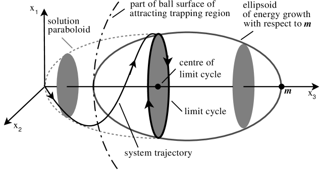
Figure 5: Solution behaviour of the system (41). The trajectories converge in spirals along the paraboloid (light grey, dashed line) toward the globally stable limit cycle (black, solid and thick line), as exemplified by one representative (black, solid, thin line). For one $\boldsymbol{m}$ with a corresponding negative definite $\mathsfbi{A}_{S}$ the trapping region of minimal radius (indicated by black, dot-dashed line) is determined by the contained ellipsoid of positive energy growth (19) (dark grey, solid, thick line).

We employ that ${\boldsymbol{m}}$ lies on the $x_{3}$-axis orthogonal to the limit cycle plane, $K_{\boldsymbol{m}}$ is seen to remain constant on the limit cycle. The limit cycle is contained in the intersection set of the infinite number of ellipsoids, each defined by a positive parameter $\epsilon>0$.

5.2 On the long-term boundedness of a POD Galerkin model

In Deane et al.  (1991) and Noack et al.  (2003), a Galerkin model for the cylinder wake flow is proposed employing the first 8 modes from a proper orthogonal decomposition (POD). The post-transient dynamics of oscillatory laminar vortex shedding at a Reynolds number of $\mbox{{Re}}=100$ in the wake is accurately resolved by this model.

The 8-dimensional Galerkin system is given by the differential equation

$$\frac{dx_{i}}{dt} = c_{i}+\sum_{j=1}^{8}l_{ij}\,x_{j}+\sum_{j,k=1}^{8}q_{ijk}\,x_{j}x_{k}.$$ (64)

The energy preservation property (4) is enforced for the quadratic term. The kinetic energy $K$ is produced in the first mode pair ($x_{1},x_{2}$) with the same positive growth rate of energy. The other six modes form pairs of the same negative energy growth rate, consuming the energy transferred by the first pair. For initial conditions close to the projection of the Navier-Stokes attractor onto the 8-dimensional subspace, the post-transient dynamics is reproduced (Noack et al. , 2003). Starting far from the limit cycle, also solutions which converge to infinity are numerically observed.

To test the criterion of theorem 1, the largest eigenvalue of the linear symmetric part ${\mathsfbi{A}}_{S}$ is minimised over a set of shift vectors ${\boldsymbol{m}}$. The optimisation has been performed via a simulated annealing algorithm (see, e.g., Gershenfeld, 2006) with random seeding in ${\boldsymbol{m}}\in[-100,100]^{8}$. This box contains the limit cycle which is centred around the origin. The box can be considered as very large, since it is almost two orders of magnitude larger then the radius of this limit cycle. In all computations, the minimum of the largest eigenvalues is positive, which indicates that the criterion cannot be fulfilled. This result is confirmed by simulations shown in Noack et al.  (2003) verifying a divergent behaviour of (64) to infinity for some initial values. Also Deane et al.  (1991) report fragile Galerkin system behaviour for a similar POD wake model. In fact, the fragility of the POD model for vortex shedding has inspired numerous enhancements of the reduced-order modelling method, e.g. a nonlinear eddy viscosity term (Cordier et al. , 2013), a stabilising spectral viscosity term (Sirisup & Karniadakis, 2004), a stabilising linear term (Galletti et al. , 2004), a stabilising additional shift mode (Noack et al. , 2003), or the inclusion of Navier-Stokes constraints construction of generalised POD modes (Balajewicz et al. , 2013).

5.3 On the long-term boundedness of a POD Galerkin model with shift mode

The 8-dimension POD model of the previous section is stabilised by including an additional shift mode ${\boldsymbol{u}}_{9}$ in the Galerkin expansion following Noack et al.  (2003, 2005). This shift mode ${\boldsymbol{u}}_{9}$ represents the normalised difference of mean flow and stationary solution. In addition, the base flow ${\boldsymbol{u}}_{0}$ is chosen to be the unstable steady solution so that the origin is the fixed point of the Navier-Stokes dynamics. In the following, long-term boundedness of the resulting 9-mode Galerkin system is proven for all initial conditions.

The dynamical system (64) is generalised by additional terms on the right-hand sides and a new additional equation arising from the shift mode:

$$\frac{dx_{i}}{dt} = \underbrace{c_{i}+\sum_{j=1}^{8}l_{ij}\,x_{j}+\sum_{j,k=1}^{8}q_{ijk}\,x_{j}x_{k}}_{\mbox{terms from the 8-mode system~{}\eqref{eq:8modemodel}}}+$$ (65a)

$$\underbrace{l_{i9}\,x_{9}+\sum_{k=1}^{8}q_{i9k}\,x_{9}x_{k}+\sum_{j=1}^{8}q_{ij9}\,x_{j}x_{9}+q_{i99}\,x_{9}^{2}}_{\mbox{additional `shift mode' terms}}\,,\;i=1,\ldots,8\,,$$

$$\frac{dx_{9}}{dt} = c_{9}+\sum_{j=1}^{9}l_{9j}\,x_{j}+\sum_{j,k=1}^{9}q_{9jk}\,x_{j}x_{k}\,.$$ (65b)

For all numerically investigated initial conditions employed in Noack et al.  (2003), the system solutions are long-term bounded and converge to a limit cycle.

In the following, we prove long-term boundedness of the 9-mode Galerkin system with the criterion of theorem 1. Learning from the mean-field model, only translations (9) along the mean-field axis are considered, i.e. ${\boldsymbol{m}}=\left(0,0,0,0,0,0,0,0,\alpha\right)^{\top}$ with $\alpha>0$. Figure 6 visualises the situation at $\alpha\approx 1$. There is a change of the sign of the largest eigenvalue of ${\mathsfbi{A}}_{S}$ from being positive to negative at $\alpha\approx 1$. By the translation, the largest eigenvalue decreases initially linearly with $\alpha$. After some value of $\alpha$, this largest eigenvalue remains negative and constant due other eigenvalues which are not affected by the translation. Thus, the largest eigenvalue of ${\mathsfbi{A}}_{S}$ remains constant for larger $\alpha$.

Figure 6: Visualisation of the criterion of theorem 1 for long-term boundedness of the 9-mode cylinder wake Galerkin system (65). Shown are the largest eigenvalue $\lambda_{1}$ of ${\mathsfbi{A}}_{S}$ of the shifted system (22) and the estimated radius $R_{m}$ of the globally attracting trapping ball $B$ described in this theorem, for several shift vectors ${\boldsymbol{m}}=\left(0,0,0,0,0,0,0,0,\alpha\right)^{\top}$ with $\alpha>0$.

In conclusion, there exist translations which make ${\mathsfbi{A}}_{S}$ negative definite. Thus, the 9-mode Galerkin system is shown to be long-term bounded because a monotonically attracting trapping region must exist according to theorem 1. Furthermore, it is shown in the figure that there is a minimum of the volume of the trapping region for a certain ${\boldsymbol{m}}$ as indicated by the curve of the estimated radius $R_{m}$ of the trapping region.

6 Design of a Trefethen-Reddy Galerkin system

In this section, we consider the Trefethen-Reddy system (Trefethen et al. , 1993) as celebrated paradigm for linear transient growth and nonlinear dynamics. This system has a non-algebraic nonlinearity, i.e. it cannot be obtained from a Galerkin method. Here, we use the criterion of theorem 1 to design an energy-preserving quadratic term with similar nonlinear behaviour.

Trefethen et al.  (1993) have proposed a simple dynamical system exhibiting important features of the non-normal linear term and nonlinearity:

$$\frac{d{\boldsymbol{x}}}{dt} = \left[\begin{array}[]{cc}-\mbox{{Re}}^{-1}&1\\ 0&-2\,\mbox{{Re}}^{-1}\end{array}\right]\,{\boldsymbol{x}}\,+\,\|{\boldsymbol{x}}\|\,\left[\begin{array}[]{cc}0&-1\\ 1&0\end{array}\right]\,{\boldsymbol{x}}\,.$$ (70)

Here, Re mimics the effect of the Reynolds number. The linear part of this Trefethen-Reddy system is represented by a non-normal matrix such that transient growth of the energy $K$ can be obtained in the linear regime. The transient growth levels increase with Re. At sufficiently large values, the nonlinear term becomes important and the following bootstrapping effect has been observed. Initial conditions ${\boldsymbol{x}}(0)=[0,const.]^{\top}$ are numerically considered. For small $\|{\boldsymbol{x}}(0)\|$, the dynamics converge to the origin with linear growth rates. For larger $\|{\boldsymbol{x}}(0)\|$, the trajectories converge to fixed points ${\boldsymbol{x}}_{S}$, $\|{\boldsymbol{x}}_{S}\|\approx 1$, with far larger growth rates than in the linear regime.

The Trefethen-Reddy system qualitatively displays important non-normal linear and nonlinear effects observed, for instance, in boundary layers and internal flows. However, (70) cannot be obtained from a Galerkin method. There exist no spatial modes ${\boldsymbol{u}}_{1}$, ${\boldsymbol{u}}_{2}$ such that the projection onto the incompressible Navier-Stokes equation yields a square root expression like $\|{\boldsymbol{x}}\|$.

The goal in this section is to model the bootstrapping effect by a long-term bounded Galerkin system of form (2), thus offering an alternative to  (70) which is arguably more physical. Hence, a new nonlinear term needs to be identified. The requested energy preservation of the quadratic term strongly limits the number of free parameters from $10$ to $2$ (see also Bourgeois et al. , 2013). The corresponding dynamical system reads

$$\frac{d{\boldsymbol{x}}}{dt} = \left[\begin{array}[]{cc}-\mbox{{Re}}^{-1}&1\\ 0&-2\,\mbox{{Re}}^{-1}\end{array}\right]\,{\boldsymbol{x}}\,+\,\delta\left(\sin\theta\left[\begin{array}[]{c}x_{1}\,x_{2}\\ -x_{1}^{2}\end{array}\right]\,+\,\cos\theta\left[\begin{array}[]{c}-x_{2}^{2}\\ x_{1}\,x_{2}\end{array}\right]\right)$$ (77)

for some $\delta>0$ and $\theta\in(0,2\pi]$. This system is of form (20) with

$${\mathsfbi{L}}_{S}\;=\;\left[\begin{array}[]{cc}-\mbox{{Re}}^{-1}&1/2\\ 1/2&-2\,\mbox{{Re}}^{-1}\end{array}\right]\,,$$ (80)

and

$${\mathsfbi{Q}}^{(1)}\;=\;\delta\left[\begin{array}[]{cc}0&2^{-1}\sin\theta\\ 2^{-1}\sin\theta&-\cos\theta\end{array}\right],\;{\mathsfbi{Q}}^{(2)}\;=\;\delta\left[\begin{array}[]{cc}-\sin\theta&2^{-1}\cos\theta\\ 2^{-1}\cos\theta&0\end{array}\right].$$ (85)

The existence of a monotonically attracting trapping region can be shown for the parameters $\theta\approx\pi/2,\pi,3\pi/2,2\pi$ as follows. For the translation vector

$${\boldsymbol{m}} = \delta^{-1}\,[\sin\theta,\cos\theta]^{\top},$$

it yields

$${\mathsfbi{A}}_{S} = \left[\begin{array}[]{cc}-\mbox{{Re}}^{-1}+2^{-1}\sin 2\theta&0\\ 0&-2\,\mbox{{Re}}^{-1}+2^{-1}\sin 2\theta\end{array}\right]\;\approx\;\left[\begin{array}[]{cc}-\mbox{{Re}}^{-1}&0\\ 0&-2\,\mbox{{Re}}^{-1}\end{array}\right].$$ (90)

At large Reynolds number Re, the same ${\boldsymbol{m}}$ can be employed to show the long-term boundedness for $\theta\in[\pi/2,\pi]$ and $\theta\in[3\pi/2,2\pi]$. Via a detailed analysis of ${\mathsfbi{A}}_{S}$ for arbitrary ${\boldsymbol{m}}$ (see the techniques applied in the appendix section B), it can be shown that the criterion of theorem 1 cannot be fulfilled for sufficient large Re and $\theta\in(0,\pi/2)$ or $\theta\in(\pi,3\pi/2)$. Hence, only a $\theta\in[\pi/2,\pi]$ or $\theta\in[3\pi/2,2\pi]$ represents a candidate to model flow attractor behaviour.

With the initial conditions of Trefethen et al.  (1993), a similar bootstrapping effect can be observed, for instance for $\theta=3\pi/2$ (see figure 7). For this angle, the modified Trefethen-Reddy system reads

$$\frac{dx_{1}}{dt} = -\mbox{{Re}}^{-1}\,x_{1}\;+x_{2}\;-\;\delta\,x_{1}\,x_{2}\,,$$ (91a)

$$\frac{dx_{2}}{dt} = -2\,\mbox{{Re}}^{-1}\,x_{2}\;+\;\delta\,x_{1}^{2}\,.$$ (91b)

The location of the fixed points scale with the parameter $\delta$. For a similar scaling like in Trefethen et al.  (1993), $\delta=12.5$ is chosen for the computations illustrated in figure 7.

Figure 7: Bootstrapping effect of the modified Trefethen-Reddy system. The evolution of $\|{\boldsymbol{x}}(t)\|$ is visualised for solutions of (91) with initial conditions $x_{1}(0)=0$, $x_{2}(0)=10^{-7},10^{-6},10^{-5},4\times 10^{-5},10^{-4},10^{-3},10^{-2}$ and for $\delta=12.5$.

In conclusion, the interval of system parameters for $\theta$ is reduced employing the criterion of theorem 1. The dynamical behaviour of the modified system coincides qualitatively with the original Trefethen-Reddy system: the bootstrapping effect is modelled via a dynamical system with the same linear term but an energy-preserving quadratic term. Contrary to the original model, such a system may arise from a Galerkin projection of a 2-mode expansion onto the Navier-Stokes equation.

7 Long-term boundedness of the Lorenz system

The existence of a monotonically attracting trapping region is demonstrated for Galerkin systems (2) with stable fixed point behaviour of the example system (8) and the stable periodic limit cycle dynamics of system (41). In this section and appendix B, more complex examples are considered. We start with the well-known Lorenz system

$$\frac{dx_{1}}{dt} = -\sigma\,x_{1}\;+\;\sigma\,x_{2}\,,$$ (92a)

$$\frac{dx_{2}}{dt} = \rho\,x_{1}\;-\;x_{2}\;-\;x_{1}\,x_{3}\,,$$ (92b)

$$\frac{dx_{3}}{dt} = -\beta\,x_{3}\;+\;x_{1}\,x_{2}\,,$$ (92c)

for positive parameters $\sigma$, $\rho$ and $\beta$. This system is of form (20) with ${\boldsymbol{c}}={\boldsymbol{0}}$, ${\mathsfbi{Q}^{(1)}}={\mathsfbi{0}}$ and

$${\mathsfbi{L}}\;=\;\left[\begin{array}[]{ccc}-\sigma&\sigma&0\\ \rho&-1&0\\ 0&0&-\beta\end{array}\right],\;{\mathsfbi{Q}^{(2)}}\;=\;\left[\begin{array}[]{ccc}0&0&-\frac{1}{2}\\ 0&0&0\\ -\frac{1}{2}&0&0\end{array}\right],\;{\mathsfbi{Q}^{(3)}}\;=\;\left[\begin{array}[]{ccc}0&\frac{1}{2}&0\\ \frac{1}{2}&0&0\\ 0&0&0\end{array}\right]\,.$$ (102)

In particular, the quadratic term is energy preserving. For Lorenz’s choice of the parameters

$$\sigma=10,\quad\rho=28,\quad\beta=8/3$$ (103)

the solution is characterised by a strange attractor. However it is known, that the solution is long-term bounded. A trapping region of ellipsoidal form can found via a Lyapunov function (Swinnerton-Dyer, 2001).

Because there are positive and negative eigenvalues of ${\mathsfbi{L}}_{S}$, there exist directions of positive and of negative energy growth $K$. However, via the quadratic term the trajectories are deflected from directions of positive energy growth to directions of negative energy growth, stabilising the resulting strange attractor (see figure 8).

The directions of energy growth and the symmetry axes of the quadratic term do not coincide. The dynamics of the system is dominated by the quadratic term in case of large deviations from the origin and far enough from fixed points of the quadratic term at the two poles and the equator. Hence, the boundedness of the system is determined by the accumulation of energy growth along the trajectories of the quadratic term crossing areas of negative and positive growth. The set of points with a vanishing quadratic term has to be investigated separately, leading to an investigation of the linear term.

+     =  

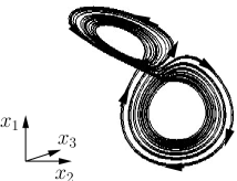
Figure 8: Fields of the symmetric part of the linear term (left) and the quadratic term (middle), and the strange attractor (right) of the Lorenz system (92) for Lorenz’s choice of system parameters.

In the following, long-term boundedness is shown with the criterion of theorem 1. After the translation employing ${\boldsymbol{m}}=[0,0,\rho+\sigma]^{\top}$ and invoking (25), the symmetric part of the transformed system is equal to

$${\mathsfbi{A}}_{S} = \left[\begin{array}[]{ccc}-\sigma&0&0\\ 0&-1&0\\ 0&0&-\beta\end{array}\right].$$ (107)

The negative definiteness of the matrix ${\mathsfbi{A}}_{S}$ proofs the existence of a monotonically attracting trapping region. Following theorem 1 further, one of these regions is given by the closed ball $B({\boldsymbol{m}},R_{m})$ with $R_{m}=\beta(\rho+\sigma)/\sqrt{\sigma}$ in case of $\sigma>\beta>1$. For Lorenz’s choice of parameters (103), the trapping region is given by $B({\boldsymbol{m}},R_{m})\approx B([0,0,38]^{\top},32)$. Hence, the complete strange attractor is situated inside of the ball $B$. It can be shown that the Lorenz system represents a prototype of the dynamics illustrated in figure 3 via further computation of the ellipsoid $E$ using (19). For large times the trajectories of the Lorenz system are pushing the boundary of the ellipsoid through and are alternately repelling from and attracting to ${\boldsymbol{m}}$.

8 Conclusions and future directions

We consider linear-quadratic dynamical systems and propose a criterion which is sufficient for long-term boundedness and necessary for globally stable attractor behaviour. For the first time, a straight-forward procedure (see figure 4) can discriminate between physical and unphysical behaviour for a generic class of Galerkin models with quadratic nonlinearity. The key enabler is a generalisation of Lyapunov’s direct method for identification of monotonically attracting trapping regions. These regions represent a more accessible property than the attractor property: the existence of monotonically attracting trapping regions is based solely on eigenvalue computations of linear combinations of system intrinsic matrices.

One distinct benefit is given for the model calibration and model reduction: unphysical systems can be identified a priori. One can avoid the computational burden of integration of the dynamical systems needed for a comprehensive set of system parameters and a large set of initial conditions.

Similarly, control laws which lead to unphysical nonlinear dynamical behaviour can be rejected a priori. A straight-forward control design is enabled via the design of monotonically attracting trapping regions. In the appendix section C, the respective control design is detailed for state stabilisation and for attractor control.

The criterion is applied to reduced-order models like the Galerkin models for a cylinder wake (Noack et al. , 2003), the Lorenz system, and modifications to show long-term boundedness or indicate unboundedness (see table 1). Furthermore the capability of the criterion to reduce complexity for parameter identification is demonstrated for the Trefethen-Reddy system. Here, a Galerkin system is identified, reproducing the bootstrapping phenomenon observed in Trefethen et al.  (1993).

Class 1 systems		Class 2 systems		Class 3 systems
9-mode Galerkin system (65)		8-mode Galerkin system (65)
for the cylinder wake,		for the cylinder wake
mean-field system (41)
Lorenz system (92)		modification (131) of Lorenz		modification (131) of Lorenz
		system for $\alpha_{1}\geq 0$		system for $\alpha_{1}<0$
’example system’ (8)		’inversed example system’ (117)
modification (77) of		modification (77) of
the Trefethen-Reddy system		the Trefethen-Reddy system
for $\theta=0,\pi/2$		for $\theta\neq 0,\pi/2$
		Rikitake system (138)
		Hamiltonian systems

Table 1: Classification of the investigated dynamical systems employing the categories introduced in figure 4.

The proposed methods are generalisable to Galerkin systems of larger dimensions in a straight-forward manner. Such systems may originate, for instance, from computational fluid dynamics. The numerical realisation of the criterion is only restricted by the current state of the art of the numerical linear algebra and multidimensional optimisation.

Appendix A Boundary conditions for the preservation property of the quadratic term

In this section, property (4) is derived for a large class of boundary conditions. The energy preservation of the quadratic term it is known for periodic boundary conditions (see, e.g. McComb, 1991; Holmes et al. , 2012) and for stationary Dirichlet conditions (Rummler, 2000). Here, we extend the range of validity also for open shear flows.

We assume an incompressible flow in a stationary domain $\Omega$ with Dirichlet, periodic or uniform free-stream conditions. $\mathbf{\xi}\in\Omega$ represents the physical location. The boundary of the domain is denoted by $\partial\Omega$.

Starting point are the quadratic Galerkin system coefficients corresponding to the convective Navier-Stokes term (see, e.g., equation (20) of the chapter ‘Galerkin method for Nonlinear Dynamics’ in Noack et al. , 2011).:

$$\tilde{q}_{ijk} := -\int_{\Omega}{\boldsymbol{u}}_{i}^{\top}\,\boldsymbol{\nabla}\boldsymbol{\cdot}\left({\boldsymbol{u}}_{j}\,{\boldsymbol{u}}_{k}^{\top}\right)d{\boldsymbol{\xi}}\,.$$ (108)

The symmetry (3) of the Galerkin system coefficients $q_{ijk}$ originated from the symmetrisation

$$q_{ijk}=\frac{1}{2}\left(\tilde{q}_{ijk}\;+\;\tilde{q}_{ikj}\right)\,.$$ (109)

It follows that equation (4) is equivalent to

$$\tilde{q}_{ijk}+\tilde{q}_{ikj}+\tilde{q}_{jik}+\tilde{q}_{jki}+\tilde{q}_{kij}+\tilde{q}_{kji}=0, i,j,k=1,\ldots,N.$$ (110)

Equation (108) is transformed by partial integration:

$$\tilde{q}_{ijk} = -\int_{\Omega}{\boldsymbol{u}}_{i}\left(\sum_{\beta=1}^{3}u_{j}^{\beta}\frac{\partial}{\partial\xi_{\beta}}{\boldsymbol{u}}_{k}\;+\;\underbrace{\left(\boldsymbol{\nabla}\boldsymbol{\cdot}{\boldsymbol{u}}_{j}\right)}_{=0}\,{\boldsymbol{u}}_{k}\right)d{\boldsymbol{\xi}}$$

$$= -\int_{\Omega}\sum_{\alpha,\beta=1}^{3}\left(u_{i}^{\alpha}u_{j}^{\beta}\frac{\partial}{\partial\xi_{\beta}}u_{k}^{\alpha}\right)d{\boldsymbol{\xi}}\,,$$

$$= -\int_{\Omega}\sum_{\alpha,\beta=1}^{3}\left(\frac{\partial}{\partial\xi_{\beta}}\left(u_{i}^{\alpha}u_{j}^{\beta}u_{k}^{\alpha}\right)\;-\;u_{k}^{\alpha}\frac{\partial}{\partial\xi_{\beta}}\left(u_{i}^{\alpha}u_{j}^{\beta}\right)\right)d{\boldsymbol{\xi}}\,,$$

$$= -\int_{\Omega}\boldsymbol{\nabla}\boldsymbol{\cdot}\left(\left({\boldsymbol{u}}_{i}{\boldsymbol{u}}_{k}\right){\boldsymbol{u}}_{j}\right)d{\bf\xi}\;+\;\int_{\Omega}\left({\boldsymbol{u}}_{i}{\boldsymbol{u}}_{k}\right)\underbrace{\boldsymbol{\nabla}\boldsymbol{\cdot}{\boldsymbol{u}}_{j}}_{=0}d{\boldsymbol{\xi}}\;+\;\int_{\Omega}\sum_{\alpha,\beta=1}^{3}u_{k}^{\alpha}u_{j}^{\beta}\frac{\partial}{\partial\xi_{\beta}}u_{i}^{\alpha}d{\boldsymbol{\xi}}\,,$$

$$= -\oint_{\partial\Omega}\left({\boldsymbol{u}}_{i}{\boldsymbol{u}}_{k}\right){\boldsymbol{u}}_{j}{\boldsymbol{\eta}}\,dS\;-\;\tilde{q}_{kji}\,,$$ (112)

where ${\boldsymbol{\eta}}$ denotes the unit outward normal at the surface $\partial\Omega$ of the considered domain $\Omega$. Here, the incompressibility of the modes $\boldsymbol{\nabla}\boldsymbol{\cdot}{\boldsymbol{u}}_{i}=0$, $i=1,\ldots,N$, is derived from the postulated incompressibility of the flow $\boldsymbol{\nabla}\boldsymbol{\cdot}{\boldsymbol{u}}$ exploiting the linearity of the Galerkin approximation (1) and of the divergence operator.

Let us assume vanishing surface integrals,

$$\oint_{\partial\Omega}\left({\boldsymbol{u}}_{i}{\boldsymbol{u}}_{j}\right){\boldsymbol{u}}_{k}=0,\quad i,j,k=1,\ldots,N.$$ (113)

Then, (112) and (113) imply

$$\tilde{q}_{ijk}=-\tilde{q}_{kji},\quad i,j,k=1,\ldots,N.$$ (114)

The energy preservation of the original and symmetrised quadratic terms, i.e. (4) and (110), can easily be derived from (114).

In the following, conditions for vanishing surface integrals (113) are determined. (113) has been shown to vanish for stationary Dirichlet conditions, implying the no-slip condition for all modes  ${\boldsymbol{u}}_{i}\equiv{\boldsymbol{0}}$ at the boundary (see, e.g. Rummler, 2000). Similarly straight-forward is the proof for periodic boundary conditions (see, e.g. McComb, 1991; Holmes et al. , 2012). Both boundary conditions may be combined, like in plane parallel Couette and Poiseuille channel flows (Rummler & Noske, 1998) or in Hagen-Poiseuille flow (Boberg & Brosa, 1988).

The proof for free-stream conditions at infinity is more challenging, as it requires certain far-wake properties of the flow. We consider flows in infinite domains around obstacles of finite extend. The integrals (113) vanish if the velocity rapidly decreases for large distances from the origin. As examples of free turbulent shear flows, nominally two-dimensional cylinder wakes, two-dimensional jets and three-dimensional circular jets are considered. Here, it is easily shown that a sequence of integrals (113) over surfaces of concentric balls $\Omega_{R}$ converge to zero, if their radii $R$ converge to infinity. As centre of the balls $\Omega_{R}$, the centre of the cylinder or the centre of the nozzle exit might by employed. An upper bound of the absolute values of the integrals is estimated via the radius, the dimension $D=2,3$ of the flow configuration and the centre line (fluctuation) velocity $u_{c}$ in streamwise direction.

The surface integral over the sphere $\Omega_{R}$ reads

$$\left|\oint_{\partial\Omega_{R}}\left({\boldsymbol{u}}_{i}{\boldsymbol{u}}_{j}\right){\boldsymbol{u}}_{k}{\boldsymbol{\eta}}\,dS\right| \leq \oint_{\partial\Omega_{k}}|{\boldsymbol{u}}_{i}||{\boldsymbol{u}}_{j}||{\boldsymbol{u}}_{k}||{\bf\eta}|\,dS\,,$$ (115)

$$\leq \sup{|{\boldsymbol{u}}_{i}|}\,\sup{|{\boldsymbol{u}}_{j}|}\,\sup{|{\boldsymbol{u}}_{k}|}|\Omega_{R}|\,,$$

$$\propto u_{c}(R)^{3}\,R^{D-1}\,.$$

Following Schlichting (1968), the centre line velocity is decreasing with radius $R$ via

$$u_{c}(R)\propto R^{\kappa}$$ (116)

where the decay rate $\kappa$ is equal to $-1/2$ for two-dimensional wakes and jets, and $\kappa=-1$ for the circular jet. Employing the estimate (115), in summary, there is a decrease of the absolute value of the integrals (113) with $R^{-1/2}$ for two-dimensional wakes and jets and with $R^{-1}$ for the three-dimensional circular jet. Hence, the integrals converge to zero for $R\to\infty$ leading to vanishing integrals over the infinite domain.

In conclusion, an intrinsic preservation property (4) exists for Galerkin systems of configurations with corresponding boundary conditions, e.g. flows around obstacles like spheres, cylinders and airfoils, in uniform stream as well as many internal flows.

Appendix B Examples of unboundedness, vanishing nonlinearity and semidefiniteness

In this section, dynamical systems (2) are discussed which do not obey the criterion for boundedness of theorem 1. The examples include a modification of the two-dimensional system (8) (subsection B.1), modified Lorenz equations (subsection B.2), and the Rikitake system (subsection B.3).

B.1 Two-dimensional system of ordinary differential equations

A first example for divergent dynamical behaviour is given from the time inversion $t\mapsto-t$ of (8). The resulting system has propagators of opposite sign and reads

$$\frac{dx_{1}}{dt} = x_{1}\;-\;x_{2}^{2}\,,$$ (117a)

$$\frac{dx_{2}}{dt} = -x_{2}\;+\;x_{1}\,x_{2}\,,$$ (117b)

where

$${\boldsymbol{c}}\;=\;\left[\begin{array}[]{c}0\\ 0\end{array}\right],\;{\mathsfbi{L}}\;=\;\left[\begin{array}[]{cc}1&0\\ 0&-1\end{array}\right],\;{\mathsfbi{Q}^{(1)}}\;=\;\left[\begin{array}[]{cc}0&0\\ 0&-1\end{array}\right],\;{\mathsfbi{Q}^{(2)}}\;=\;\left[\begin{array}[]{cc}0&\frac{1}{2}\\ \frac{1}{2}&0\end{array}\right].$$ (126)

The long-term behaviour of system (117) is investigated employing the criterion of theorem 1. Invoking (25) and employing the matrices (126), the symmetric part of the shift transformed system is determined to be

$${\mathsfbi{A}}_{S} = \left[\begin{array}[]{cc}1&-{m_{2}}/2\\ -{m_{2}}/2&m_{1}-1\end{array}\right].$$ (129)

The larger eigenvalue of ${\mathsfbi{A}}_{S}$

$$\lambda_{1} = \frac{1}{2}\left(m_{1}+\sqrt{(2-m_{1})^{2}+m_{2}^{2}}\right)$$

is positive: $\lambda_{1}\geq 1$ is concluded from $|2-m_{1}|\geq 2-m_{1}$ because

$$m_{1}+\sqrt{(2-m_{1})^{2}+m_{2}^{2}}\geq m_{1}+|2-m_{1}|\geq 2.$$ (130)

Hence, a monotonically attracting trapping region and a globally stable attractor do not exist. By numerical system integration, a divergent behaviour to infinity is observed for large times.

B.2 Modified Lorenz system

Similarly, the following modification of the Lorenz system

$$\frac{dx_{1}}{dt} = \alpha_{1}\,x_{1}\,,$$ (131a)

$$\frac{dx_{2}}{dt} = \alpha_{2}\,x_{2}\;-\;x_{1}\,x_{3}\,,$$ (131b)

$$\frac{dx_{3}}{dt} = \alpha_{3}\,x_{3}\;+\;x_{1}\,x_{2}\,,$$ (131c)

with $-\infty<\alpha_{1},\alpha_{2},\alpha_{3}<\infty$ is considered for investigation of existence of monotonically attracting trapping regions and of globally stable attractors. From equation (25) we get

$${\mathsfbi{A}}_{S} = \left[\begin{array}[]{ccc}\alpha_{1}&-m_{3}/2&m_{2}/2\\ -m_{3}/2&\alpha_{2}&0\\ m_{2}/2&0&\alpha_{3}\end{array}\right].$$ (135)

Independently of the choice of ${\boldsymbol{m}}$, the sum of the three eigenvalues of ${\mathsfbi{A}}_{S}$ is equal to the constant trace of ${\mathsfbi{A}}_{S}$, i.e. the mean value $\gamma=(\lambda_{1}+\lambda_{2}+\lambda_{3})/3$ is constant. The eigenvalues are increasingly separated with growing $|m_{2}|$, $|m_{3}|$ which can be seen from the dispersion of the eigenvalues

$$\frac{1}{3}\sum\limits_{i=1}^{3}(\lambda_{i}-\gamma)^{2}\;=\;\frac{1}{3}\left(\sum\limits_{i=1}^{3}\lambda_{i}^{2}\right)-\gamma^{2} = f(\alpha_{1},\alpha_{2},\alpha_{3})+\frac{m_{2}^{2}+m_{3}^{2}}{6}.$$ (136)

For derivation of (136), Vieta’s formula for the characteristic polynomial of ${\mathsfbi{A}}_{S}$

$$(\lambda-\alpha_{1})\,(\lambda-\alpha_{2})\,(\lambda-\alpha_{3})\;-\;\frac{m_{2}^{2}}{4}\,(\lambda-\alpha_{2})\;-\;\frac{m_{3}^{2}}{4}\,(\lambda-\alpha_{3})$$

is employed, which yields

$$\frac{3}{2}\gamma^{2}-\frac{1}{2}(\lambda_{1}^{2}+\lambda_{2}^{2}+\lambda_{3}^{2})\;=\;\lambda_{1}\lambda_{2}+\lambda_{2}\lambda_{3}+\lambda_{1}\lambda_{3}\;=\;\alpha_{1}\alpha_{2}+\alpha_{2}\alpha_{3}+\alpha_{1}\alpha_{3}-\frac{m_{2}^{2}+m_{3}^{2}}{4}\,.$$

From the increased dispersion of the eigenvalues and the preservation of the mean value, the following can be concluded: If one of the three growth rates $\alpha_{i}$ is positive, then for each ${\boldsymbol{m}}$ there is always at least one $\lambda_{i}$ positive as well. Following theorem 1, a monotonically attracting trapping region does not exist in that case. This result is easily validated considering the dynamics in case that one eigenvalue is positive. For $\alpha_{1}>0$, the variable $x_{1}$ is diverging to infinity for large times. For $\alpha_{1}<0$ and large times the quadratic term is small compared to the linear term and the variable $x_{i}$ with positive $\alpha_{i}$ is diverging to infinity. If $\alpha_{1}=0$, $x_{1}$ is constant in time for each initial value, i.e. a monotonically trapping region does not exist either.

In the case $\alpha_{1}<0$, the nonlinear term of the system (131) is vanishing for large times. Invoking theorem 2, under action of an additional antisymmetric part, there might exist globally attracting trapping regions or fixed points which are not monotonically attracting. One example with an additional antisymmetric linear term is

$$\frac{dx_{1}}{dt} = \alpha_{1}\,x_{1},$$ (137a)

$$\frac{dx_{2}}{dt} = \alpha_{2}\,x_{2}\;-\;x_{3}\;-\;x_{1}\,x_{3},$$ (137b)

$$\frac{dx_{3}}{dt} = \alpha_{3}\,x_{3}\;+\;x_{2}\;+\;x_{1}\,x_{2}.$$ (137c)

The analysis for a monotonically attracting region is de facto the same like in system (131). However, if $\alpha_{1}<0$, the application of linear theory is enabled by the vanishing of the nonlinear term for large times. Only the evolution equations for $x_{2}$ and $x_{3}$ are considered while the nonlinear term is neglected. Here, $[x_{2},x_{3}]^{\top}=[0,0]^{\top}$ is a globally stable fixed point, if and only if the real parts of the eigenvalues of $\left[\begin{array}[]{cc}\alpha_{2}&-1\\ 1&\alpha_{3}\end{array}\right]$ are negative-valued. In conclusion, in case of a vanishing nonlinearity, linear analyses are needed in addition for a complete analysis of the long-term boundedness of the system.

B.3 The Rikitake system

The criterion of theorem 1 cannot be generalised from negative definite matrices ${\mathsfbi{A}}_{S}$ to negative semidefinite matrices ${\mathsfbi{A}}_{S}$ in a straight-forward manner. As a corresponding example, a modified Rikitake system

$$\frac{dx_{1}}{dt} = -\nu\,x_{1}\;+\;x_{2}\,x_{3}\,,$$ (138a)

$$\frac{dx_{2}}{dt} = -\alpha\,x_{1}\;-\;\nu\,x_{2}\;+\;x_{1}\,x_{3}\,,$$ (138b)

$$\frac{dx_{3}}{dt} = \theta\;-\omega\;x_{1}\,x_{2}\,,$$ (138c)

is utilised with the positive parameters $\nu$ and $\alpha$ (Goriely & Hyde, 1998). In the traditional Rikitake system, $\theta=1$ and $\omega=1$ are chosen. Here $\omega$ is set to $\omega=2$ to fulfil the postulation (3). From similar analyses like above, the positive semidefiniteness of the largest eigenvalue, i.e. $\lambda_{1}\geq 0$, of ${\mathsfbi{A}}_{S}$ can be shown. In the following, ${\boldsymbol{m}}=[0,0,\alpha/2]^{\top}$ is considered, where $\lambda_{1}=0$ and $\lambda_{2}=\lambda_{3}=-\nu$ because

$${\mathsfbi{A}}_{S} = \left[\begin{array}[]{ccc}-\nu&0&0\\ 0&-\nu&0\\ 0&0&0\end{array}\right].$$ (142)

We leave $\theta=1$ at first. Here, it is known that there is a simple solution ${\boldsymbol{x}}=\left[0,0,t\right]^{\top}$ which is diverging to infinity for larges times. However for $\theta=0$, long-term boundedness is immediately ensured invoking the evolution equation (11) for the chosen ${\mathsfbi{A}}_{S}$ and ${\boldsymbol{d}}={\boldsymbol{0}}$: the energy $K_{\boldsymbol{m}}$ cannot grow in any direction. This means that for negative semidefinite ${\mathsfbi{A}}_{S}$ additional information, e.g. of the constant term might be crucial for long-term boundedness analyses.

Appendix C Large-deviation and attractor control

C.1 General considerations

In this section, applications of the criterion of section 4 for control design are sketched.

For control, the term ${\mathsfbi{B}}\,{\boldsymbol{b}}(t)$ is added to the right side of the Galerkin system (20) leading to

$$\frac{d{\boldsymbol{x}}}{dt} = {\boldsymbol{c}}+{\mathsfbi{L}}\,{\boldsymbol{x}}+{\mathsfbi{B}}\,{\boldsymbol{x}}+\left[\,{\boldsymbol{x}}^{\top}\,{\mathsfbi{Q}}^{(1)}\,{\boldsymbol{x}}\,,\ldots,\,{\boldsymbol{x}}^{\top}\,{\mathsfbi{Q}}^{(N)}\,{\boldsymbol{x}}\,\right]^{\top}\;+\;{\mathsfbi{B}}\,{\boldsymbol{b}}\,$$ (143)

with the input matrix ${\mathsfbi{B}}$ and the input vector ${\boldsymbol{b}}={\boldsymbol{b}}(t)$. Let us assume full-state feedback with constant, linear and quadratic terms

$${\boldsymbol{b}} = {\boldsymbol{c}}^{b}+{\mathsfbi{L}}^{b}\,{\boldsymbol{x}}+\left[\,{\boldsymbol{x}}^{\top}\,{\mathsfbi{Q}}^{b(1)}\,{\boldsymbol{x}}\,,\ldots,\,{\boldsymbol{x}}^{\top}\,{\mathsfbi{Q}}^{b(N)}\,{\boldsymbol{x}}\,\right]^{\top}$$ (144)

with the free coefficients in ${\boldsymbol{c}}^{b}$, ${\mathsfbi{L}}^{b}$ and ${\mathsfbi{Q}}^{b(i)}$. The actuation term reads

$${\mathsfbi{B}}\,{\boldsymbol{b}}(t)={\boldsymbol{c}}^{g}+{\mathsfbi{B}}^{g}\,{\boldsymbol{x}}+\left[\,{\boldsymbol{x}}^{\top}\,{\mathsfbi{Q}}^{g(1)}\,{\boldsymbol{x}}\,,\ldots,\,{\boldsymbol{x}}^{\top}\,{\mathsfbi{Q}}^{g(N)}\,{\boldsymbol{x}}\,\right]^{\top}\,,$$ (145)

introducing the feedback vector ${\boldsymbol{c}}^{g}$, the feedback matrix ${\mathsfbi{L}}^{g}$, and the symmetric matrices ${\mathsfbi{Q}}^{g(i)}$ for the quadratic term of feedback. We request that the control law (144) is chosen to respect the energy preservation property

$$q^{g(i)}_{jk}+q^{g(j)}_{ik}+q^{g(k)}_{ij} = 0,\quad i,j,k=1,\ldots,N\,.$$ (146)

In summary, the actuated system reads

$$\frac{d{\boldsymbol{x}}}{dt} = {\boldsymbol{c}}^{a}+{\mathsfbi{L}}^{a}\,{\boldsymbol{x}}+\left[\,{\boldsymbol{x}}^{\top}\,{\mathsfbi{Q}}^{a(1)}\,{\boldsymbol{x}}+{\boldsymbol{x}}^{\top}\,{\mathsfbi{Q}}^{a(N)}\,{\boldsymbol{x}}\,\right]^{\top},$$ (147)

where ${\boldsymbol{c}}^{a}={\boldsymbol{c}}+{\boldsymbol{c}}^{g}$, ${\mathsfbi{L}}^{a}={\mathsfbi{L}}+{\mathsfbi{L}}^{g}$, and ${\mathsfbi{Q}}^{a(i)}={\mathsfbi{Q}}^{(i)}+{\mathsfbi{Q}}^{g(i)}$, $i=1,\ldots,N$. The controlled system is of form (20) and thus contained in the class of dynamical systems considered in this paper. That’s why the long-term behaviour of the corresponding dynamics can be investigated by the criterion of theorem 1. In control design, the choice of the parameters ${\boldsymbol{c}}^{b}$, ${\mathsfbi{L}}^{b}$ and ${\mathsfbi{Q}}^{b(i)}$, $i=1,\ldots,N$, is restricted by constraints implied by the input matrix ${\mathsfbi{L}}^{g}$.

Two tasks are pursued here

1. Large-deviation control: The purpose of this part is twofold. One goal is the modification of the parameters of system (20) such that the existence of a monotonically attracting trapping region is ensured. On the other hand, artefacts like blow-ups in model-based control design are precluded a priori.

2. Attractor control: Target is the manipulation of statistical attractor moments. Thereto, in this paper, tools are provided to design the volume and the location of monotonically attracting trapping regions. In one extreme case, on which is focused here, a globally attracting fixed point is designed, i.e. the attractor mean is equal to a fixed point and the higher central moments are zero. Focus of large deviation control is the identification or creation of monotonically attracting trapping regions. This can be achieved as described in section 4.

As one extreme case of attractor control, we assume a constant actuation, i.e. vanishing $\mathsfbi{L}^{b}$ and $\mathsfbi{Q}^{b(i)}$. The feedback vector ${\boldsymbol{c}}^{g}$ may be chosen such that each state ${\boldsymbol{m}}\in{\mathcal{S}}$ is a globally attracting fixed point of the feedback system. This implies

$$0=\,{\boldsymbol{c}}^{a}_{i}+\sum_{j=1}^{N}l_{ij}\,m_{j}-\sum_{j,k=1}^{N}q^{(i)}_{jk}\,m_{j}m_{k}\,, i=1,\ldots,N\,.$$ (148)

Then, the energy $K_{\boldsymbol{m}}$ represents a Lyapunov function, because the linear symmetric part ${\mathsfbi{A}}_{S}$ is negative definite. The choice of the feedback vector ${\boldsymbol{c}}^{g}$ might be restricted such that a globally stable fixed point is not attainable due to the constraints implied by the input matrix ${\mathsfbi{L}}^{g}$ of the flow control configuration. However even in this case, the first and second attractor moments can be estimated from the location and the volume of the trapping region. Thus, the moments can be manipulated by the design of the ellipsoid of energy growth given by equation (19). The effort of a corresponding volume force actuation for this attractor control might be large. A trade-off between the attractor scaling via choice of ${\boldsymbol{c}}^{g}$ and the above discussed design of ${\mathcal{S}}$ might be necessary for model-based flow control applications.

Examples for the application of large deviation and attractor control are discussed in the following.

C.2 Example for large deviation control

For large deviation control, the set ${\mathcal{S}}$ of stabilisable states is analytically or numerically created and designed for the example of system (8) endowed with a linear feedback matrix of the family of linear symmetric matrices

$${\mathsfbi{L}}^{g}_{\boldsymbol{\beta}}:=\left[\begin{array}[]{cc}\beta_{1}&0\\ 0&\beta_{2}\end{array}\right]\,.$$ (151)

The corresponding sets ${\mathcal{S}}_{\beta}$ of stabilisable states ${\bf m}$ are identified via auxiliary calculations to be

$${\mathcal{S}}_{\boldsymbol{\beta}}=\begin{cases}\left\{{\boldsymbol{x}}=[x_{1},x_{2}]^{\top}:\;x_{1}>1+\beta_{2},\,|x_{2}|<2\sqrt{1-\beta_{1}}\sqrt{x_{1}-1-\beta_{2}}\right\}&\mbox{ for }\beta_{1}<1,\\ \emptyset&\mbox{ for }\beta_{1}\geq 1\,.\end{cases}$$ (152)

In particular, ${\mathcal{S}}_{\boldsymbol{0}}:=\left\{{\boldsymbol{x}}=[x_{1},x_{2}]^{\top}:\;x_{1}>1,\,|x_{2}|<2\sqrt{x_{1}-1}\right\}$. Starting from ${\mathcal{S}}_{\boldsymbol{0}}$, the set ${\mathcal{S}}_{\boldsymbol{\beta}}$ is designed via variation of ${\boldsymbol{\beta}}$ as demonstrated in figure 9. If the set ${\mathcal{S}}={\mathcal{S}}_{\boldsymbol{\beta}}$ is not empty, the long-term dynamics of the resulting system is bounded invoking theorem 1.

In the case $\beta_{1}\geq 1$, the set of stabilisable states is empty and a monotonically attracting trapping region does not exist, which is obvious considering the resulting system

$$\frac{dx_{1}}{dt} = \left(\beta_{1}-1\right)x_{1}\;+\;x_{2}^{2}\,,$$ (153)

$$\frac{dx_{2}}{dt} = \left(1+\beta_{2}\right)x_{2}\;-\;x_{1}\,x_{2}\,,$$ (154)

in the subspace of the $x_{1}$-axis, i.e. $x_{2}=0$. It means, that the ${\mathsfbi{L}}^{g}_{\boldsymbol{\beta}}$ with $\beta_{1}\geq 1$ cannot be chosen to form a control with bounded system behaviour.

Figure 9: Design of the open set ${\mathcal{S}}_{\boldsymbol{\beta}}$ of stabilisable states at the left side of the curve. By variation of the parameters ${\boldsymbol{\beta}}=[\beta_{1},\beta_{2}]^{\top}$ of the feedback matrix ${\mathsfbi{L}}^{g}_{\boldsymbol{\beta}}$, the set ${\mathcal{S}}_{\boldsymbol{\beta}}$ is modified via a widening/narrowing (varying $\beta_{1}$) of the right opening angle of the set or a spatial shift in $x_{1}$-direction (via varying $\beta_{2}$).

C.3 Example for attractor control

As attractor control example, we control the size of the monotonically attracting trapping region. The Lorenz system (92) is extended by a control vector ${\boldsymbol{c}}^{g}=\gamma\left[0,0,\beta(\rho+\sigma)\right]^{\top}$ with $\gamma\in[0,1]$ such that

$$\frac{d{\boldsymbol{x}}}{dt} = \gamma\left[\begin{array}[]{c}0\\ 0\\ \beta\left(\rho+\sigma\right)\end{array}\right]+\left[\begin{array}[]{ccc}-\sigma&\sigma&0\\ -\rho&-1&0\\ 0&0&-\beta\end{array}\right]{\boldsymbol{x}}+\left[\begin{array}[]{c}0\\ -x_{1}\,x_{3}\\ x_{1}\,x_{2}\end{array}\right]\,.$$ (164)

For $\gamma=0$, this system is identical to the Lorenz equations (92). From the transformation shift of ${\boldsymbol{m}}=[0,0,\rho+\sigma]^{\top}$ to the origin, the system for ${\boldsymbol{y}}={\boldsymbol{x}}-{\boldsymbol{m}}$ is obtained:

$$\frac{d{\boldsymbol{y}}}{dt} = \left(\gamma-1\right)\left[\begin{array}[]{c}0\\ 0\\ \beta\left(\rho+\sigma\right)\end{array}\right]+\left[\begin{array}[]{ccc}-\sigma&\sigma&0\\ -\sigma&-1&0\\ 0&0&-\beta\end{array}\right]{\boldsymbol{y}}+\left[\begin{array}[]{c}0\\ -y_{1}\,y_{3}\\ y_{1}\,y_{2}\end{array}\right]$$ (174)

For $\gamma=1$ the constant part of the right side is equal to zero. Thus, the energy is a Lyapunov function and ${\boldsymbol{m}}$ is a globally stable fixed point in this case. Generally, the equation (19) for the ellipsoid of positive energy growth is given in original coordinates by

$$\frac{x_{1}^{2}}{\alpha_{1}^{2}}+\frac{x_{2}^{2}}{\alpha_{2}^{2}}+\frac{\left(x_{3}-\left(\rho+\sigma\right)+\left(\gamma-1\right)\left(\rho+\sigma\right)/2\right)^{2}}{\alpha_{3}^{2}} = 1$$ (175)

with the half-axes

$$\alpha_{1}\,=\,\left(1-\gamma\right)\frac{\rho+\sigma}{2\sqrt{\sigma}},\;\alpha_{2}\,=\,\left(1-\gamma\right)\frac{\rho+\sigma}{2},\;\alpha_{3}\,=\,\left(1-\gamma\right)\frac{\rho+\sigma}{2\sqrt{\beta}}\,.$$ (176)

Hence, the half-axes are shrinking linearly with the growth of $\gamma$. This is true as well as for the radius of the monotonically attracting trapping region given by the smallest ball with ${\boldsymbol{m}}$ at the centre which contains the ellipsoid.

In conclusion, the attractor contained in this trapping region is shrinking, and degenerates to a fixed point for $\gamma=1$. The first statistical moment situated in the ball is converging to ${\boldsymbol{m}}$ for $\gamma\to 1$, the standard deviation bounded by the ball radius is converging to zero. For $\gamma\approx 0.288$ there is a transition from the strange attractor to three fixed points which converge for $\gamma\to 1$ to the monotonically stable fixed point ${\boldsymbol{m}}$ at $\gamma=1$. Thus, the control parameter $\gamma$ defines a transition scenario between stationary and chaotic dynamical behaviour!

References

- Aamo & Krstić (2002) Aamo, O. M. & Krstić, M. 2002 Flow Control by Feedback: Stabilization and Mixing. Springer-Verlag, London.
- Balajewicz et al. (2013) Balajewicz, M., Dowell, E. & Noack, B. R. 2013 Low-dimensional modelling of high-Reynolds-number shear flows incorporating constraints from the Navier-Stokes equation. J. Fluid Mech. 729, 285–308.
- Boberg & Brosa (1988) Boberg, L. & Brosa, U. 1988 Onset of turbulence in a pipe. Z. Naturforsch. A 43, 697–726.
- Bourgeois et al. (2013) Bourgeois, J., Noack, B. R. & Martinuzzi, R. 2013 Generalised phase average with applications to sensor-based flow estimation of the wall-mounted square cylinder wake. Accepted for publication in Journal of Fluid Mechanics.
- Cazemier et al. (1998) Cazemier, W., Verstappen, R. W. C. P. & Veldman, A. E. P. 1998 Proper orthogonal decomposition and low-dimensional models for driven cavity flows. Phys. Fluids 7, 1685–1699.
- Cordier et al. (2013) Cordier, L., Noack, B. R., Daviller, G., Lehnasch, G., Tissot, G., Balajewicz, M & Niven, R. 2013 Control-oriented model identification strategy. Exp. Fluids 54, 1580.
- Deane et al. (1991) Deane, A. E., Kevrekidis, I. G., Karniadakis, G. E. & Orszag, S. A. 1991 Low-dimensional models for complex geometry flows: Application to grooved channels and circular cylinders. Phys. Fluids A 3, 2337–2354.
- Drazin & Reid (1981) Drazin, P. G. & Reid, H. W. 1981 Hydrodynamic stability. Cambridge University Press, Cambridge.
- Fletcher (1984) Fletcher, C. A. J. 1984 Computational Galerkin Methods. Springer, New York.
- Galdi & Padula (1990) Galdi, G. P. & Padula, M. 1990 A new approach to the energy theory in the stability of fluid motion. Arch. Rational Mech. Anal. 22, 163–184.
- Galletti et al. (2004) Galletti, G., Bruneau, C. H., Zannetti, L. & Iollo, A. 2004 Low-order modelling of laminar flow regimes past a confined square cylinder. J. Fluid Mech. 503, 161–170.
- Gerhard et al. (2003) Gerhard, J., Pastoor, M., King, R., Noack, B. R., Dillmann, A., Morzyński, M. & Tadmor, G. 2003 Model-based control of vortex shedding using low-dimensional Galerkin models. AIAA-Paper 2003-4262.
- Gershenfeld (2006) Gershenfeld, N. 2006 The Nature of Mathematical Modeling. Cambridge University Press, Cambridge.
- Goriely & Hyde (1998) Goriely, A. & Hyde, C. 1998 Finite-time blow up in dynamical systems. Phys. Lett. A 250, 311–318.
- Guckenheimer & Holmes (1986) Guckenheimer, J. & Holmes, P. 1986 Nonlinear Oscillations, Dynamical Systems, and Bifurcations of Vector Fields. Springer, New York.
- Holmes et al. (2012) Holmes, P., Lumley, J. L., Berkooz, G. & Rowley, C. W. 1998 Turbulence, Coherent Structures, Dynamical Systems and Symmetry. Cambridge University Press, Cambridge, 2nd edition.
- Joseph (1976) Joseph, D. D. 1976 Stability in fluid motions I, II. Springer Tracts in Natural Philosophy 27–28, Springer-Verlag, New York.
- Khalil (2002) Khalil, H. K. 2002 Nonlinear Dynamics. Dover Publications, New York.
- Kim & Bewley (2007) Kim, J. & Bewley, T. 2007 A linear systems approach to flow control. Ann. Rev. Fluid Mech. 39, 383–417.
- Kolda & Bader (2009) Kolda, T. G. & Bader, B. W. 1998 Tensor decompositions and applications. SIAM Rev. 51(3), 455–500.
- Ladyz̆henskaya (1963) Ladyz̆henskaya, O. A. 1963 The Mathematical Theory of Viscous Incompressible Flow. Gordon and Breach, New York.
- Lyapunov (1892) Lyapunov, A. M. 1892 Stability of Motion. Academic Press, London, New York.
- McComb (1991) McComb, W. D. 1991 The Physics of Fluid Turbulence. Claredon Press, Oxford.
- Meiss (2007) Meiss, J. D. 2007 Differential Dynamical Systems. Series ’Monographs on Mathematical Modelling and Computation’ 14, Society for Industrial and Applied Mathematics, Philadelphia.
- Noack & Eckelmann (1994) Noack, B. R. & Fasel, H 1994 A global stability analysis of the steady and periodic cylinder wake. J. Fluid Mech. 270, 297–330.
- Noack et al. (2003) Noack, B. R., Afanasiev, K., Morzyński, M., Tadmor, G. & Thiele, F. 2003 A hierarchy of low-dimensional models for the transient and post-transient cylinder wake. J. Fluid Mech. 497, 335–363.
- Noack et al. (2005) Noack, B. R., Papas, P. & Monkewitz, P. A. 2005 The need for a pressure-term representation in empirical Galerkin models of incompressible shear flows. J. Fluid Mech. 523, 339–365.
- Noack et al. (2008) Noack, B. R., Schlegel, M., Ahlborn, B., Mutschke, G., Morzyński, M., Comte, P. & Tadmor, G. 2008 A finite-time thermodynamics of unsteady fluid flows. J. Non-Equilib. Thermodyn. 33 (2), 103–148.
- Noack et al. (2010) Noack, B. R., Schlegel, M., Morzyński, M. & Tadmor, G. 2010 System reduction strategy for Galerkin models of fluid flows. Int. J. Numer. Meth. Fluids 63, 231–248.
- Noack et al. (2011) Noack, B. R., Morzyński, M. & Tadmor, G. 2011 Reduced-Order Modelling for Flow Control. Series ’CISM International Centre for Mechanical Sciences’ 528, Springer, Wien, New York.
- Rempfer & Fasel (1994) Rempfer, D. & Fasel, H. F. 1994 Dynamics of three-dimensional coherent structures in a flat-plate boundary layer. J. Fluid Mech. 275, 257–283.
- Rummler & Noske (1998) Rummler, B. & Noske, A. 1998 Direct Galerkin Approximation of Plane-Parallel-Couette and Channel Flows by Stokes Eigenfunctions. Notes Numer. Fluid Mech. 64, 3–19.
- Rummler (2000) Rummler, B. 2000 Zur Lösung der instationären inkompressiblen Navier-Stokesschen Gleichungen in speziellen Gebieten (transl: On the solution of the incompressible Navier-Stokes equations in some domains). Habilitation thesis, Fakultät für Mathematik, Otto-von-Guericke-Universität, Magdeburg.
- Samimy et al. (2007) Samimy, M., Debiasi, M., Caraballo, E., Serrani, A., Yuan, X., Little, J. & Myatt, J. 2010 Feedback control of subsonic cavity flows using reduced-order models. J. Fluid Mech. 579, 315–346.
- Schlegel et al. (2009) Schlegel, M., Noack, B. R., Comte, P., Kolomenskiy, D., Schneider, K., Farge, M., Scouten, J., Luchtenburg, D. M., & Tadmor, G. 2009 Reduced-order modelling of turbulent jets for noise control. In Brun, C., Juvé, D., Manhart, M., Munz, C.-D. (editors), Numerical Simulation of Turbulent Flows and Noise Generation, Series ’Notes on Numerical Fluid Mechanics and Multidisciplinary Design (NNFM)’ 104, Springer-Verlag, 3–27.
- Schlegel et al. (2012) Schlegel, M., Noack, B. R., Jordan, P., Dillmann, A., Gröschel, E., Schröder, W., Wei, M., Freund, J. B., Lehmann, O. & Tadmor, G. 2012 On least-order flow representations for aerodynamics and aeroacoustics. J. Fluid Mech. 697, 367–398.
- Schlichting (1968) Schlichting, H. 1968 Boundary-layer theory. McGraw-Hill, 3rd english edition.
- Schmid & Henningson (2001) Schmid, P. J. & Henningson, D. S. 2001 Stability and Transition in Shear Flows. Applied Mathematical Sciences 142, Springer, New York.
- Sipp et al. (2010) Sipp, D., Marquet, O., Meliga, P. & Barbagallo, A. 2010 Dynamics and control of global instabilities in open flows: a linearized approach. Appl. Mech. Rev. 63, 030801.
- Sirisup & Karniadakis (2004) Sirisup, S. & Karniadakis, G. E. 2004 A spectral viscosity method for correcting the long-term behavior of POD models. J. Comp. Phys. 194, 92–116.
- Straughan (2004) Straughan, B. 2004 The Energy Method, Stability and Nonlinear Convection. Applied Mathematical Sciences 94, 2nd ed., Springer-Verlag, New York.
- Swinnerton-Dyer (2000) Swinnerton-Dyer, P. 2000 A note on Liapunov’s method. Dynam. Stabil. Syst. 15, 3–10.
- Swinnerton-Dyer (2001) Swinnerton-Dyer, P. 2001 Bounds for trajectories of the Lorenz equations: an illustration of how to choose Liapunov functions. Phys. Lett. A 281, 161–167.
- Trefethen et al. (1993) Trefethen, L. N., Trefethen, A. E., Reddy, S. C. & Driscoll, T. A. 1993 Hydrodynamic stability without eigenvalues. Science 261, 578–584.
- Trefethen & Embree (2005) Trefethen, L. N. & Embree, M. 2005 Spectra and Pseudospectra. Princeton University Press, New Jersey.
- Wei & Rowley (2009) Wei, M. & Rowley, C. W. 2009 Low-dimensional models of a temporally evolving free shear layer. J. Fluid Mech. 618, 113–134.
- Willcox & Megretski (2005) Willcox, K. & Megretski, A. 2005 Fourier Series for Accurate, Stable, Reduced-Order Models in Large-Scale Applications. SIAM J. Sci. Comput. 26(3), 944–962.