Towards a Unified Description of the Intergalactic Medium at Redshift $z\approx 2.5$

Abstract

We examine recent measurements of the $z\approx 2.5$ intergalactic medium (IGM) which constrain the H I frequency distribution $f(N_{\rm HI})$ and the mean free path $\lambda_{\rm mfp}^{912}$ to ionizing radiation. We argue that line-blending and the clustering of strong absorption-line systems have led previous authors to systematically overestimate the effective Lyman limit opacity, yielding too small of a $\lambda_{\rm mfp}^{912}$ for the IGM. We further show that recently published measurements of $f(N_{\rm HI})$ at $N_{\rm HI}\approx 10^{16}\,{\rm cm^{-2}}$ lie in strong disagreement, implying underestimated uncertainty from sample variance and/or systematics like line-saturation. Allowing for a larger uncertainty in the $f(N_{\rm HI})$ measurements, we provide a new cubic Hermite spline model for $f(N_{\rm HI})$ which reasonably satisfies all of the observational constraints under the assumption of randomly distributed absorption systems. We caution, however, that this formalism is invalid in light of absorber clustering and use a toy model to estimate the effects. Future work must properly account for the non-Poissonian nature of the IGM.

1 Introduction

The intergalactic medium (IGM, revealed by the Ly$\alpha$ forest) is the diffuse medium of gas and metals which traces the large-scale density fluctuations of the universe. These fluctuations were imprinted in primordial density perturbations and, therefore, their analysis offers unique constraints on cosmology, especially on scales of tens to hundreds of Mpc. Modern observations of the IGM – via absorption-line analysis of distant quasars – has provided several probes of the $\Lambda$CDM paradigm including: a measurement of its matter power spectrum, upper limits to the mass of neutrinos, and an independent measure of baryonic acoustic oscillations (e.g. McDonald et al., 2005; Viel et al., 2009; Slosar et al., 2013).

These analyses leverage the statistical power of high-dispersion, high signal-to-noise (S/N) spectra from a select set of sightlines (e.g. Croft et al., 2002; Bergeron et al., 2004; Rudie et al., 2012), together with low-dispersion, lower S/N spectra on many thousands of sightlines (Schneider et al., 2010; Pâris et al., 2012; Lee et al., 2013). Concurrently, these datasets provide a precise characterization of fundamental properties of the IGM. This includes statistics on the opacity of the Ly$\alpha$ forest (e.g. Croft et al., 2002; Faucher-Giguère et al., 2008b; Palanque-Delabrouille et al., 2013; Becker et al., 2013), the incidence of optically thick gas (aka Lyman limit systems or LLS, Prochaska et al., 2010; Ribaudo et al., 2011; Fumagalli et al., 2013b; O’Meara et al., 2013, hereafter O13), and the H I column densities ($N_{\rm HI}$) of the strongest, damped Ly$\alpha$ systems (DLAs; Prochaska et al., 2005; Prochaska & Wolfe, 2009; Noterdaeme et al., 2012). Traditionally, many of these results have been described by a single distribution function $f(N_{\rm HI})$ defined at a given redshift and often normalized to the absorption length $dX=\frac{H_{0}}{H(z)}(1+z)^{2}dz$ introduced by Bahcall & Peebles (1969).

In principle, $f(N_{\rm HI})$ encodes the primary characteristics of the IGM and its evolution with cosmic time. This includes an estimation of the mean free path to ionizing radiation $\lambda_{\rm mfp}^{912}$, defined as the most likely proper distance a packet of ionizing photons will travel before suffering an $\rm e^{-1}$ attenuation. Under the standard assumption of randomly distributed absorbers, one may calculate the effective Lyman limit opacity $\tau_{\rm eff,LL}$ as follows. An ionizing photon with $h\nu_{\rm em}\geq 1$Ryd emitted from a quasar with redshift $z_{\rm em}$ will redshift to 1 Ryd at $z_{912}\equiv(\nu_{\rm 912}/\nu_{\rm em})(1+z_{\rm em})-1$. The effective optical depth that this photon experiences from Lyman limit continuum opacity is then (cf. Meiksin & Madau, 1993):

$$\tau_{\rm eff,LL}(z_{912},z_{\rm em})=\int\limits_{z_{912}}^{z_{\rm em}}\int\limits_{0}^{\infty}f(N_{\rm HI},z^{\prime})\{1-\exp\left[\,-N_{\rm HI}\sigma_{\rm ph}(z^{\prime})\,\right]\}dN_{\rm HI}dz^{\prime}\;\;\;,$$ (1)

where $\sigma_{\rm ph}$ is the photoionization cross-section evaluated at the photon frequency $\nu=\nu_{912}(1+z^{\prime})/(1+z_{912})$. For a given $z_{\rm em}$, one may measure $\lambda_{\rm mfp}^{912}$ by solving for the redshift $z_{912}$ where $\tau_{\rm eff,LL}=1$ and converting the offset from $z_{\rm em}$ to a proper distance.

In a series of recent papers, we have introduced an alternate method to estimating $\lambda_{\rm mfp}^{912}$ using composite quasar spectra, which directly assess the average IGM opacity to ionizing photons (Prochaska et al., 2009; O’Meara et al., 2013; Fumagalli et al., 2013b; Worseck & Others, 2013). These ‘stacks’ reveal the average, intrinsic quasar spectrum (its spectral energy distribution or SED) as attenuated by the IGM. Provided one properly accounts for several other, secondary effects on the composite spectrum at rest wavelengths $\lambda_{r}<912$Å (e.g. the underlying slope of the quasar SED), it is straightforward to directly measure $\lambda_{\rm mfp}^{912}$ and estimate uncertainties from standard bootstrap techniques. One may then use estimates of $\lambda_{\rm mfp}^{912}$ to independently constrain $f(N_{\rm HI})$ via Equation 1, especially at column densities where $f(N_{\rm HI})$ is most difficult to estimate directly, i.e. at $N_{\rm HI}\approx 10^{15}-10^{17}\,{\rm cm^{-2}}$ where the Lyman series lines lie on the flat portion of the curve-of-growth and the Lyman limit opacity $\tau_{\rm 912}\ll 1$. In this manner, we concluded that $f(N_{\rm HI})$ is relatively flat at $N_{\rm HI}\la 10^{17.5}\,{\rm cm^{-2}}$ and steepens at lower column densities (Prochaska et al., 2010; O’Meara et al., 2013, see also Ribaudo et al. 2011). These constraints may be compared against predictions from numerical simulations to constrain models of galaxy formation and astrophsyical processes related to radiative transfer (e.g. McQuinn et al., 2011; Altay et al., 2013).

Most recently, Rudie et al. (2013, hereafter R13) have published a study on $f(N_{\rm HI})$ for $N_{\rm HI}\approx 10^{12}-10^{17}\,{\rm cm^{-2}}$ using the traditional approach of performing Voigt profile fits to “lines” in quasar spectra. From their unique dataset, in terms of S/N and spectral coverage, they report a high incidence of lines with $N_{\rm HI}\approx 10^{16}\,{\rm cm^{-2}}$. Using the incidence of LLS to extrapolate their results to higher $N_{\rm HI}$, R13 infer a much smaller mean free path at $z=2.4$ ($147\pm 15\,\rm h_{70}^{-1}\,Mpc$) than the direct measurement ($242\pm 42\,\rm h_{70}^{-1}\,Mpc$; O13). Such a disagreement is unseemly in this era of precision cosmology and IGM characterization.

More importantly, the difference has significant implications for estimations of the intensity $J_{\nu}^{\rm EUVB}$ of the extragalactic ultraviolet background (EUVB), the escape fraction from galaxies, studies of He II reionization, and models of the circumgalactic medium of galaxies (e.g. Fumagalli et al., 2011; Compostella et al., 2013; Nestor et al., 2013; Dixon et al., 2013; Becker & Bolton, 2013). For example, a favored approach to evaluating $J_{\nu}^{\rm EUVB}$ is to calculate the attenuation of known sources of ionizing radiation by the IGM (Haardt & Madau, 1996; Faucher-Giguère et al., 2008a; Haardt & Madau, 2012). A difference in $\lambda_{\rm mfp}^{912}$ of a factor of 2 leads directly to a 100% uncertainty in $J_{\nu}^{\rm EUVB}$. Similarly, a much lower $\lambda_{\rm mfp}^{912}$ value yields a systematically higher escape fraction from medium-band imaging below the Lyman limit (e.g. Nestor et al., 2013).

In the following, we explore this apparent conflict and propose several explanations to reconcile the measurements. Furthermore, we offer new insight into the meaning and limitations of $f(N_{\rm HI})$ and its validity as a description of the IGM. Throughout the manuscript, we adopt a $\Lambda$CDM cosmology with $\Omega_{\Lambda}=0.7$, $\Omega_{m}=0.3$ and $H_{0}=70h_{70}\,\rm km\,s^{-1}\,Mpc^{-1}$ and we have translated previous measurements to this cosmology where necessary.

2 Controversies in the $z\approx 2.5$ IGM

In this section, we examine the primary observational constraints on $f(N_{\rm HI})$ and $\lambda_{\rm mfp}^{912}$ in the $z\approx 2.5$ IGM and highlight tension between the measurements.

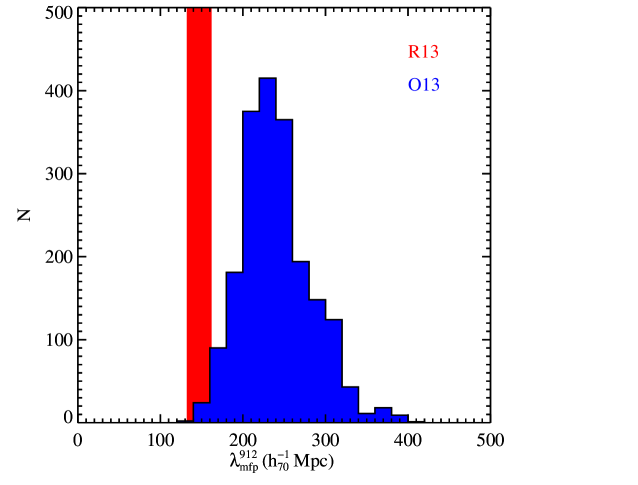
Figure 1: The blue histogram shows the distribution of $\lambda_{\rm mfp}^{912}$ values measured from the O13 quasar composite spectrum, adopting their bootstrap analysis and a $\Lambda$CDM cosmology with $\Omega_{\Lambda}=0.7$, $\Omega_{m}=0.3$ and $H_{0}=70h_{70}\,\rm km\,s^{-1}\,Mpc^{-1}$. We measure a mean value $\lambda_{\rm mfp}^{912}=242\pm 42\rm h_{70}^{-1}\,Mpc$. The red band shows the R13 estimate of $\lambda_{\rm mfp}^{912}$: $147\pm 15\rm h_{70}^{-1}\,Mpc$. Only 31/2000 of the trials fall within $1\sigma$ of the R13 value.

2.1 Comparison of the Published MFP Values

There are two recently published values for the MFP to ionizing photons at $z\approx 2.4$, derived from two distinct techniques: (1) an evaluation based on the measured, average attenuation of flux in a composite quasar spectrum ($242\pm 42\,\rm h_{70}^{-1}\,Mpc$; O13); and (2) the value derived by R13 ($147\pm 15\,\rm h_{70}^{-1}\,Mpc$) from their new constraints on $f(N_{\rm HI})$, old estimations of the incidence of LLS, and an assumed redshift evolution in the line density of strong absorbers $\ell(z)\propto(1+z)^{\gamma_{\ell}}$. R13 fitted a disjoint, double power-law model to the $f(N_{\rm HI})$ constraints, generated IGM models with standard Monte Carlo techniques, and assessed the predicted flux attenuation to estimate $\lambda_{\rm mfp}^{912}$ and its uncertainty. Treating the uncertainty in each measurement as a Gaussian, the two diverge at 97%c.l. The uncertainty in $\lambda_{\rm mfp}^{912}$ from O13 is non-Gaussian, however, with a significant tail to higher values. Figure 1 shows 2000 bootstrap evaluations of $\lambda_{\rm mfp}^{912}$ from O13, rerun with the cosmology adopted here. The average value is $242\pm 42\,\rm h_{70}^{-1}\,Mpc$, and we find that only 31/2000 trials have $\lambda_{\rm mfp}^{912}$ within $1\sigma$ of the R13 value (shaded region).

Worseck et al. (2013) have recently analyzed the redshift evolution of $\lambda_{\rm mfp}^{912}$ combining all of the $z>2$ measurements made from quasar composite spectra. They find the values are well modeled by a single power-law $\lambda_{\rm mfp}^{912}(z)=\lambda_{\rm mfp,z=4}^{912}[(1+z)/5]^{\eta}$ with $\lambda_{\rm mfp,z=4}^{912}=35\,\rm h_{70}^{-1}\,Mpc$ and $\eta=-5.45$. This gives $\lambda_{\rm mfp}^{912}=244\rm h_{70}^{-1}\,Mpc$ at $z=2.5$, exceeding the R13 value at very high confidence. Similarly, previous estimations based on evolution in the incidence of LLS (e.g. Songaila & Cowie, 2010) yields larger values than that reported by R13, as illustrated by R13 (their Figure 15). We conclude that the O13 and R13 measurements of $\lambda_{\rm mfp}^{912}$ at $z\approx 2.5$ are highly discrepant. We do note that the quasars sampled by R13 have emission redshifts 0.2 to 0.3 higher than the quasars of O13 and also systematically large luminosities. We do not believe, however, that this drives any of the differences in the derived IGM properties.

2.2 Modeling the Quasar Composite Spectrum

We further examine the tension between O13 and R13 with the methodology used by O13 to measure $\lambda_{\rm mfp}^{912}$. Those authors fit a $z\approx 2.5$ quasar composite spectrum at rest wavelengths $\lambda_{r}<912$Å with a five parameter model: (i) a power-law tilt to the assumed Telfer quasar template (Telfer et al., 2002), ${\delta\alpha_{\rm T}}$; (ii) the normalization of the quasar SED at $\lambda_{r}=912$Å, $C_{\rm T}$; (iii) the redshift evolution of the integrated Lyman series opacity, $\gamma_{\tau}$; and (iv,v) the normalization and redshift evolution of $\lambda_{\rm mfp}^{912}$ which O13 parameterized in terms of an opacity:

$${\tilde{\kappa}}_{912}(z)=\tilde{\kappa}_{912}(z_{\rm em})\left[\,\frac{1+z}{1+z_{\rm em}}\,\right]^{\gamma_{\kappa}}\;\;\;.$$ (2)

The resultant values of $\tilde{\kappa}_{912}(z_{\rm em})$ and $\gamma_{\kappa}$ provide an estimate for the mean free path (Figure 1).

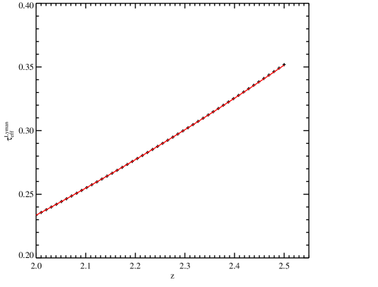
Figure 2: Plot of the predicted effective optical depth of the full H I Lyman series $\tau_{\rm eff}^{\rm Lyman}$ assuming the $f(N_{\rm HI})$ model of R13 and a uniform Doppler parameter $b=24\,{\rm km~{}s^{-1}}$. The red curve is an assumed power-law description of the values, $\tau_{\rm eff}^{\rm Lyman}(z)=\tau_{\rm eff,z=2}^{\rm Lyman}[(1+z)/3]^{\gamma_{\tau}}$ with $\gamma_{\tau}=2.65$.

We can use the same methodology to find the best-fitting model of the quasar composite spectrum, constrained to yield the $\lambda_{\rm mfp}^{912}$ value reported by R13. This model adopts the same redshift evolution of the frequency distribution of the IGM assumed by R13. Specifically, R13 assumed $\gamma_{\ell}=1$ for the redshift evolution in the incidence of strong absorbers ($N_{\rm HI}>10^{15.1}\,{\rm cm^{-2}}$) and $\gamma_{\ell}=2.5$ for lower $N_{\rm HI}$ lines. Empirically, we find that this implies $\gamma_{\tau}\approx 2.65$ (Figure 2). Finally, the parameter ${\delta\alpha_{\rm T}}$ was allowed to freely vary between $[-0.8,0]$ and we let $C_{\rm T}$ vary by $\pm 10\%$, following O13.

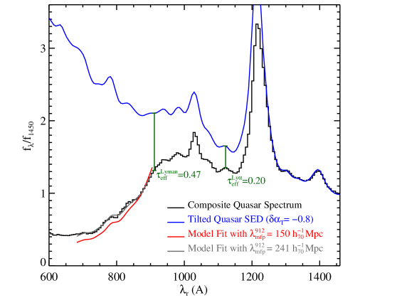
Figure 3: The black curve is the composite quasar spectrum constructed by O13 from their HST/WFC3 observations of 53 quasars at $z\approx 2.5$. Overplotted at $\lambda_{r}=680-910$Å as a gray curve is the best-fit model of O13 which corresponds to a mean free path $\lambda_{\rm mfp}^{912}=242\,\rm h_{70}^{-1}\,Mpc$. The red curve is the best-fit model forced to yield the $\lambda_{\rm mfp}^{912}=150\,\rm h_{70}^{-1}\,Mpc$ value of R13. It is a very poor description of the data. The blue curve is the intrinsic quasar SED for the $\lambda_{\rm mfp}^{912}=150\,\rm h_{70}^{-1}\,Mpc$ model, restricted to match the data at 1450Å. It is the Telfer quasar template (Telfer et al., 2002) “tilted” by ${\delta\alpha_{\rm T}}=-0.8$ with $f^{\rm SED}_{\lambda}=f_{\lambda}^{\rm Telfer}(\lambda/1450\,{\rm\AA})^{\delta\alpha_{\rm T}}$. This quasar SED yields an acceptable measurement for the effective Ly$\alpha$ opacity $\tau_{\rm eff}^{\rm Ly\alpha}$ at $\lambda_{r}\approx 1100$Å but exceeds the effective Lyman series opacity $\tau_{\rm eff}^{\rm Lyman}$ at $\lambda_{r}=912$Å predicted by R13. A quasar SED with ${\delta\alpha_{\rm T}}=-2$ would yield an acceptable model of the composite spectrum at $\lambda_{r}<912$Å having $\lambda_{\rm mfp}^{912}=150\rm h_{70}^{-1}\,Mpc$ but would greatly overpredict $\tau_{\rm eff}^{\rm Ly\alpha}$ and $\tau_{\rm eff}^{\rm Lyman}$.

Figure 3 compares the $z=2.44$ composite spectrum of O13 with the ‘best’ model having $\lambda_{\rm mfp}^{912}=152\rm h_{70}^{-1}\,Mpc$. We find that the most extreme tilt of the quasar SED (${\delta\alpha_{\rm T}}=-0.8$) is favored, but even with this rather extreme SED the resultant model is a very poor description of the data. If we adopt the RMS of the composite flux assessed from a bootstrap analysis (O13; their figure 8) and assume a Gaussian PDF, we measure $\chi_{\nu,\rm min}^{2}=2.22$ for the $\nu=33$ degrees of freedom from the 37 pixels spanning $\lambda_{r}=650-910$Å. This implies that the model is ruled out at high significance (99.99%c.l). Note however that the scatter in the composite is not truly Gaussian and the flux is highly correlated by the nature of continuum opacity. Nevertheless, we conclude that the $\lambda_{\rm mfp}^{912}$ value inferred by R13 either violates the O13 quasar composite spectrum or requires a tilt to the SED that contradicts other measurements (see also $\S$ 3.1).

Table 1: $f(N_{\rm HI})$ Constraints at $z\approx 2.5$

Constraint	$z^{a}$	log $N_{\rm HI}$	Valueb	Comment	Reference
Lya Forest	2.30	12.75–13.00	$-11.08^{+0.02}_{-0.01}$	Grabbed from astro-ph on August 30, 2013	K13
		13.00–13.25	$-11.44^{+0.02}_{-0.02}$
		13.25–13.50	$-11.80^{+0.02}_{-0.02}$
		13.50–13.75	$-12.16^{+0.02}_{-0.02}$
		13.75–14.00	$-12.51^{+0.03}_{-0.02}$
		14.00–14.25	$-12.99^{+0.03}_{-0.03}$
		14.25–14.50	$-13.46^{+0.05}_{-0.04}$
		14.50–14.75	$-13.78^{+0.05}_{-0.04}$
		14.75–15.06	$-14.29^{+0.07}_{-0.06}$
		15.06–15.50	$-14.93^{+0.06}_{-0.05}$
		15.50–16.00	$-15.97^{+0.12}_{-0.10}$
		16.00–16.50	$-16.67^{+0.17}_{-0.12}$
		16.50–17.00	$-17.22^{+0.18}_{-0.12}$
		17.00–17.50	$-17.90^{+0.23}_{-0.15}$
		17.50–18.00	$-19.17^{+0.40}_{-0.30}$
Lya Forest	2.37	13.01–13.11	$-11.33^{+0.02}_{-0.03}$	Provided by G. Rudie on Aug 28, 2013	R13
		13.11–13.21	$-11.48^{+0.02}_{-0.03}$
		13.21–13.32	$-11.65^{+0.02}_{-0.03}$
		13.32–13.45	$-11.76^{+0.02}_{-0.02}$
		13.45–13.59	$-11.96^{+0.02}_{-0.03}$
		13.59–13.74	$-12.23^{+0.03}_{-0.03}$
		13.74–13.90	$-12.53^{+0.03}_{-0.03}$
		13.90–14.08	$-12.78^{+0.03}_{-0.03}$
		14.08–14.28	$-13.11^{+0.03}_{-0.04}$
		14.28–14.50	$-13.41^{+0.04}_{-0.04}$
		14.50–14.73	$-13.74^{+0.04}_{-0.04}$
		14.73–15.00	$-14.20^{+0.05}_{-0.05}$
		15.00–15.28	$-14.75^{+0.06}_{-0.07}$
		15.28–15.60	$-15.19^{+0.07}_{-0.08}$
		15.60–15.94	$-15.66^{+0.08}_{-0.09}$
		15.94–16.32	$-16.25^{+0.09}_{-0.12}$
		16.32–16.73	$-16.91^{+0.11}_{-0.16}$
		16.73–17.20	$-17.37^{+0.11}_{-0.15}$
Lya Forest	2.34	12.50–13.00	$-11.16^{+0.04}_{-0.04}$	Recalculated for our Cosmology	K02
		13.00–13.50	$-11.73^{+0.05}_{-0.05}$
		13.50–14.00	$-12.51^{+0.07}_{-0.07}$
		14.00–14.50	$-13.27^{+0.10}_{-0.09}$
SLLS	2.51	19.00–19.60	$-20.60^{+0.19}_{-0.17}$	Only 30 systems total	OPB07
		19.60–20.30	$-21.48^{+0.23}_{-0.20}$
DLA	2.51	20.30–20.50	$-21.80^{+0.06}_{-0.06}$	$z=[2.3,2.7]$; modest SDSS bias (see Noterdaeme et al., 2009)?	PW09
		20.50–20.70	$-22.26^{+0.08}_{-0.08}$
		20.70–20.90	$-22.38^{+0.08}_{-0.07}$
		20.90–21.10	$-22.85^{+0.11}_{-0.10}$
		21.10–21.30	$-23.33^{+0.15}_{-0.15}$
		21.30–21.50	$-23.58^{+0.16}_{-0.15}$
		21.50–21.70	$-24.30^{+0.34}_{-0.30}$
		21.70–21.90	$-24.98^{+0.76}_{-0.52}$
		21.90–22.10	$-99.00^{+-99.00}_{--24.60}$
		22.10–22.30	$-99.00^{+-99.00}_{--24.80}$

Table 2: continued

$f(N_{\rm HI})$ Constraints at $z\approx 2.5$ DLA 2.50 20.10–20.20 $-21.49^{+0.05}_{-0.05}$ Tablulated N12 20.20–20.30 $-21.61^{+0.05}_{-0.05}$ 20.30–20.40 $-21.70^{+0.05}_{-0.05}$ 20.40–20.50 $-21.84^{+0.05}_{-0.05}$ 20.50–20.60 $-22.00^{+0.05}_{-0.05}$ 20.60–20.70 $-22.16^{+0.05}_{-0.05}$ 20.70–20.80 $-22.34^{+0.05}_{-0.05}$ 20.80–20.90 $-22.53^{+0.05}_{-0.05}$ 20.90–21.00 $-22.69^{+0.05}_{-0.05}$ 21.00–21.10 $-22.93^{+0.05}_{-0.05}$ 21.10–21.20 $-23.13^{+0.05}_{-0.05}$ 21.20–21.30 $-23.30^{+0.05}_{-0.05}$ 21.30–21.40 $-23.60^{+0.06}_{-0.06}$ 21.40–21.50 $-23.83^{+0.07}_{-0.07}$ 21.50–21.60 $-24.03^{+0.08}_{-0.08}$ 21.60–21.70 $-24.22^{+0.08}_{-0.08}$ 21.70–21.80 $-24.64^{+0.12}_{-0.12}$ 21.80–21.90 $-24.87^{+0.18}_{-0.18}$ 21.90–22.00 $-25.62^{+0.53}_{-0.53}$ 22.00–22.20 $-26.07^{+0.53}_{-0.53}$ 22.20–22.40 $-26.27^{+0.53}_{-0.53}$ $\ell(X)_{\tau\geq 2}$ 2.23 $>17.49$ $0.30\pm 0.07$ OPW12 $\tau_{\rm eff}^{\rm Ly\alpha}$ 2.40 12.00–17.00 $0.198\pm 0.007$ Converted to $\tau_{\rm eff}^{\rm Ly\alpha}$ from $D_{A}$. No LLS, no metals. K05 $\lambda_{\rm mfp}^{912}$ 2.44 12 – 22 $242\pm 41\,\rm h_{70}^{-1}\,Mpc$ OPW13

^aEffective redshift where the constraint was determined.
^b$f(N_{\rm HI})$ constraints are given in log.
Note: there were two modifications to the $f(N_{\rm HI})$ data from N12 (see text).
KT97: Kirkman & Tytler (1997); K01: Kim et al. (2001); K02: Kim et al. (2002); K05: Kirkman et al. (2005); OPB07: O’Meara et al. (2007); PW09: Prochaska & Wolfe (2009); OPW13: O’Meara et al. (2013); N12: Noterdaeme et al. (2012)

2.3 Tension in $f(N_{\rm HI})$

Ostensibly, the above analysis suggests that the R13 and O13 data lie in strong conflict. Thus far, however, we have only considered the $\lambda_{\rm mfp}^{912}$ and $\gamma_{\ell}$ values reported/assumed by R13 and not their actual measurements or model of $f(N_{\rm HI})$. In this spirit, we perform a joint analysis of $f(N_{\rm HI})$ imposing all of the constraints included by O13 and adding the R13 measurements. As a reminder, the constraints adopted by O13 were (see also Table 1): (1) the O13 estimate of $\lambda_{\rm mfp}^{912}$ revised for cosmology (Figure 1); (2) the mean opacity of the Ly$\alpha$ forest (Kirkman et al., 2005); (3) the incidence of $\tau\geq 2$ LLS (Ribaudo et al., 2011, O13); (4) the $f(N_{\rm HI})$ measurements of Kim et al. (2002, hereafter K02); (5) the $f(N_{\rm HI})$ measurements of strong absorption systems from O’Meara et al. (2007) and Prochaska & Wolfe (2009).

Before proceeding to model the combined R13 and O13 constraints, we examine the $f(N_{\rm HI})$ models published by R13 and O13 tested by one another’s data. Each model, of course, gives good statistical results ($\chi_{\nu}^{2}\approx 1$) for fits to the data analyzed in each paper. R13 favored a 4-parameter, disjoint set of two power-laws split at $N_{\rm HI}=10^{15.14}\,{\rm cm^{-2}}$. This model yields an acceptable $\chi^{2}_{\nu}=1.44$ for their own measurements, but gives $\chi^{2}_{\nu}=22.3$ for the O13 constraints alone (including Kim et al., 2002) and $\chi^{2}_{\nu}=11.3$ for the combined constraints (O13 plus R13). Here a substantial contribution to the $\chi^{2}$ is from the absorption systems with largest $N_{\rm HI}$ values, which R13 did not include in their analysis. Therefore, the R13 model is ruled out at very high confidence. Similarly, the O13 model (a 6-parameter, continuous set of power-laws) gives $\chi^{2}_{\nu}=11.1$ for the combined datasets driven entirely by the R13 measurements (especially those at low $N_{\rm HI}$ values).

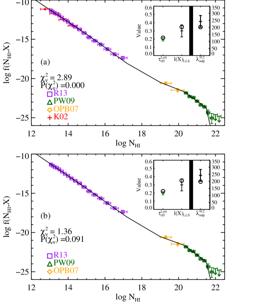
Figure 4: (a) The black curve shows a 7-parameter continuous, power-law fit with MCMC techniques to the $f(N_{\rm HI})$ constraints labeled (Table 1 Rudie et al., 2013; Prochaska & Wolfe, 2009; O’Meara et al., 2007; Kim et al., 2002) and the integral constraints in the inset (Kirkman et al., 2005; O’Meara et al., 2013). This model yields an unacceptably high reduced $\chi^{2}_{\nu}$, driven primarily by the $f(N_{\rm HI})$ values at low $N_{\rm HI}$. (b) Same as (a) but without the K02 measurements. The resultant $\chi_{\nu}^{2}$ may be considered acceptable, but we stress that this model is under great tension between the $f(N_{\rm HI})$ measurements at $N_{\rm HI}\approx 10^{17}\,{\rm cm^{-2}}$, the $\ell(X)$ constraint, and the $\lambda_{\rm mfp}^{912}$ value.

Given these ‘failed’ models, one is motivated to ask whether any $f(N_{\rm HI})$ model can fit all of the available data at $z\approx 2.5$. We proceed to fit the constraints used by O13 together with the measurements of R13 with a continuous series of power-laws with log normalization $k_{12}$ at $N_{\rm HI}=10^{12}\,{\rm cm^{-2}}$ and with breaks at five $N_{\rm HI}$ ‘pivots’ motivated by the data: $\log N_{\rm HI}^{\rm pivot}=[15.14,17.2,19.0,20.3,21.5]$. Each segment has a slope $\beta$ labeled by the pivot.

We fit this 7-parameter model to the observations using a Markov Chain Monte Carlo (MCMC; Metropolis-Hastings) algorithm, employing a 0.025 step-size for each parameter. Random initializations and multiple long MCMC chains were generated to insure proper convergence. Figure 4a presents the best-fit model (see Table 3) which has a $\chi^{2}_{\nu}=2.89$ with a probability $P(\chi_{\nu}^{2})<10^{-5}$ indicating a very poor description of the observations. The deviation is driven primarily by the $f(N_{\rm HI})$ values of K02 at low $N_{\rm HI}$. Therefore, we repeat the analysis without the K02 measurements, noting that the R13 data cover the lower $N_{\rm HI}$ range on their own, and recover the model shown in Figure 4b. The $\chi^{2}_{\nu}$ is notably improved and may even be considered acceptable, but the figure also emphasizes the tension between R13 and O13. The $\lambda_{\rm mfp}^{912}$, $\ell(X)_{\tau\geq 2}$, and $f(N_{\rm HI})\ga 10^{16.5}\,{\rm cm^{-2}}$ measurements are all poorly described by this model. We conclude that there is substantial tension between the various measurements of the IGM when one attempts to model these with a single $f(N_{\rm HI})$ model.

Table 3: $f(N_{\rm HI})$ MCMC Results

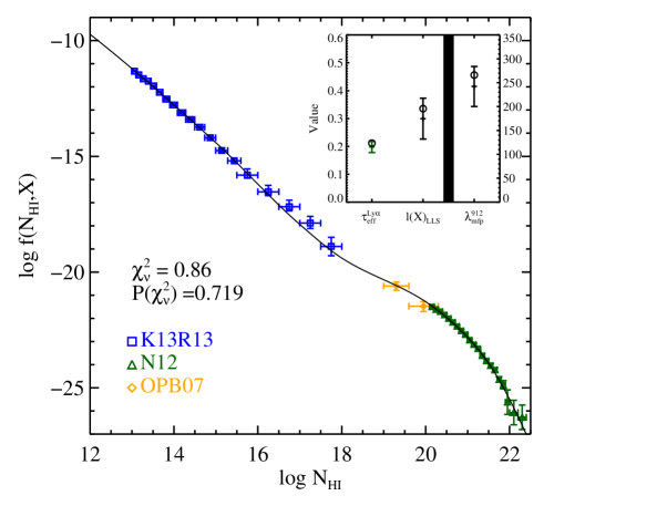
Figure 7: The black curve shows the best-fit model of $f(N_{\rm HI})$ to all of the constraints presented (see Table 1). For the $f(N_{\rm HI})$ measurements, we have adopted the values of R13 at $N_{\rm HI}<10^{15.5}\,{\rm cm^{-2}}$ but have combined their model with the K13 values at higher $N_{\rm HI}$ and adopted a larger uncertainty (see text). The resultant model is a reasonable description of the data.

Parameter	Prior	Median	16th%	84th%
Results for R13 and O13 (Figure 4a)
$k_{12}$	$U(-\infty,\infty)$	$-9.65$	0.03	0.02
$\beta_{12}$	$U(-\infty,\infty)$	$-1.57$	0.01	0.02
$\beta_{15.14}$	$U(-\infty,\infty)$	$-1.68$	0.05	0.05
$\beta_{17.2}$	$U(-\infty,\infty)$	$-1.39$	0.12	0.09
$\beta_{19}$	$U(-\infty,\infty)$	$-0.83$	0.12	0.13
$\beta_{20.3}$	$U(-\infty,\infty)$	$-1.75$	0.14	0.09
$\beta_{21.5}$	$U(-\infty,\infty)$	$-11.65$	1.64	6.35
Results for R13 and O13 without K02 (Figure 4b)
$k_{12}$	$U(-\infty,\infty)$	$-9.59$	0.02	0.03
$\beta_{12}$	$U(-\infty,\infty)$	$-1.60$	0.02	0.01
$\beta_{15.14}$	$U(-\infty,\infty)$	$-1.66$	0.04	0.05
$\beta_{17.2}$	$U(-\infty,\infty)$	$-1.42$	0.11	0.11
$\beta_{19}$	$U(-\infty,\infty)$	$-0.82$	0.12	0.13
$\beta_{20.3}$	$U(-\infty,\infty)$	$-1.74$	0.14	0.09
$\beta_{21.5}$	$U(-\infty,\infty)$	$-12.86$	2.71	7.45
Results for 8-parameter model (R13 and O13 without K02)
$k_{12}$	$U(-\infty,\infty)$	$-9.58$	0.03	0.03
$\beta_{12}$	$U(-\infty,\infty)$	$-1.61$	0.02	0.01
$\beta_{15.14}$	$U(-\infty,\infty)$	$-1.64$	0.02	0.08
$\beta_{17.2}$	$U(-\infty,\infty)$	$-2.11$	1.30	0.33
$\beta_{18.0}$	$U(-\infty,\infty)$	$-0.50$	0.56	1.29
$\beta_{19.0}$	$U(-\infty,\infty)$	$-1.04$	0.20	0.19
$\beta_{20.3}$	$U(-\infty,\infty)$	$-1.80$	0.07	0.18
$\beta_{21.5}$	$U(-\infty,\infty)$	$-9.64$	1.18	1.97
Results for Spline Model (Figure 7)
$k_{12}$	$U(-\infty,\infty)$	$-9.72$	0.04	0.07
$k_{15}$	$U(-\infty,\infty)$	$-14.41$	0.02	0.02
$k_{17}$	$U(-\infty,\infty)$	$-17.94$	0.08	0.13
$k_{18}$	$U(-\infty,\infty)$	$-19.39$	0.16	0.10
$k_{20}$	$U(-\infty,\infty)$	$-21.28$	0.03	0.03
$k_{21}$	$U(-\infty,\infty)$	$-22.82$	0.02	0.02
$k_{21.5}$	$U(-\infty,\infty)$	$-23.95$	0.03	0.04
$k_{22}$	$U(-\infty,\infty)$	$-25.50$	0.15	0.10

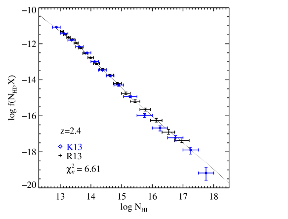
Figure 5: Comparison of the independent $f(N_{\rm HI})$ measurements for the IGM at $z=2.4$ by Kim et al. (2013, K13; blue) and Rudie et al. (2013, R13; black). Although the two groups use similar techniques on similar quality spectra (with a few notable differences), the two sets of results are highly inconsistent with one another, especially at the extrema. For example, the best-fit $f(N_{\rm HI})$ model of R13 (dotted line) has a $\chi_{\nu}^{2}=6.61$ and $P(\chi_{\nu}^{2})<10^{-5}$ when applied to the K13 measurements. This model also fails when restricting the comparison to $N_{\rm HI}>10^{15.5}\,{\rm cm^{-2}}$. We conclude that there is a significant, systematic uncertainty in assessing $f(N_{\rm HI})$ at $N_{\rm HI}>10^{15}\,{\rm cm^{-2}}$ that was unaccounted for by these authors.

In fact, the situation becomes untenable if one includes the recent measurements of $f(N_{\rm HI})$ published by Kim et al. (2013, hereafter K13). Those authors performed a similar line-profile fitting analysis to R13 of high S/N, echelle quasar spectra using standard Voigt-profile fitting techniques. They considered fewer constraints from higher order Lyman series lines than R13, but argued that this had minimal effect on their results. Figure 5 compares the two datasets. The values are in reasonably good agreement at modest $N_{\rm HI}$ values when Ly$\alpha$ and/or Ly$\beta$ are unsaturated. At larger and lower $N_{\rm HI}$ values, however, the two sets of measurements are highly inconsistent. For example, the $f(N_{\rm HI})$ model of R13 yields a $\chi_{\nu}^{2}$ on the K13 measurements which implies the two measurements disagree at greater than $99.999\%$c.l. (Figure 5). Even if we restrict the comparison to measurements with $N_{\rm HI}>10^{15.5}\,{\rm cm^{-2}}$, the R13 model gives $\chi_{\nu}^{2}=3$ and $P(\chi^{2}_{\nu})=0.018$. Not surprisingly, we cannot find any $f(N_{\rm HI})$ model that satisfactorily fits the suite of K13, R13, and O13 constraints on the IGM at $z\approx 2.5$.

3 Resolutions

We explore three ways to reconcile the conflict among the observational constraints of the $z\approx 2.5$ IGM, as described in the previous section. Each of these may contribute to a resolution: (1) O13 have overestimated $\lambda_{\rm mfp}^{912}$ by underestimating the spectral slope of the average quasar SED and/or by suffering from a statistical fluctuation; (2) line-blending has led to the double counting of absorption systems and also implies a substantial systematic uncertainty for $f(N_{\rm HI})$; (3) the clustering of absorption systems with $\tau_{\rm 912}\ga 1$ drives the evaluation of Equation 1 to underestimate $\lambda_{\rm mfp}^{912}$.

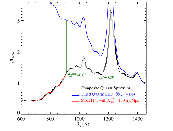
Figure 6: Similar to Figure 3 but allowing the quasar SED tilt ${\delta\alpha_{\rm T}}$ to hold any value. In this case, the quasar composite spectrum (black) may be modeled by an IGM with $\lambda_{\rm mfp}^{912}=150\rm h_{70}^{-1}\,Mpc$ (red curve) provided ${\delta\alpha_{\rm T}}<-1.5$. However, the resultant values for the effective optical depths of Ly$\alpha$ and the full Lyman series ($\tau_{\rm eff}^{\rm Ly\alpha}$, $\tau_{\rm eff}^{\rm Lyman}$) vastly exceed previous measurements (Kirkman et al., 2005; O’Meara et al., 2013). Furthermore, the implied quasar spectral slope $f^{\rm QSO}_{\nu}\propto\nu^{0.1}$ is steeper than any previous estimation and over-predicts the X-ray to optical ratio by over an order-of-magnitude.

3.1 Additional Error

Regarding the O13 analysis, it is possible to achieve a good model of the composite spectrum with $\lambda_{\rm mfp}^{912}=150\,\rm h_{70}^{-1}\,Mpc$ if one allows for an even more extreme tilt of the intrinsic quasar SED, i.e. ${\delta\alpha_{\rm T}}<-1.5$ (Figure 6). This same model, however, overpredicts both the average Ly$\alpha$ opacity $\tau_{\rm eff}^{\rm Ly\alpha}$ at $\lambda_{r}\approx 1120$Å and especially the integrated Lyman series opacity $\tau_{\rm eff}^{\rm Lyman}$ at $\lambda_{r}\approx 912$Å. Furthermore, this quasar SED would have $f_{\nu}\propto\nu^{\alpha}$ with $\alpha>0$ in the far-UV, exceeding any plausible estimation for quasars (Lusso et al., 2013). Therefore, we strongly disfavor this explanation.

Systematic error in both the K13 and R13 studies is a major concern, especially in light of the large differences between the two measurements (Figure 5). As discussed in $\S$ 2.3, there is likely a large systematic error in evaluating $f(N_{\rm HI})$ at $N_{\rm HI}\approx 10^{16}\,{\rm cm^{-2}}$ with traditional line-fitting. This is evident simply from the dispersion in results from the various studies. We conclude that there is substantial systematic error in assessing lines on the flat portion of the curve-of-growth which was not accounted for by these authors. It could be related to line-saturation (i.e. limited coverage of the complete Lyman series), line-blending (see below), or even to sample variance. Blind analysis of mock spectra may help to resolve these issues and we encourage such a study. We also recommend that future works restrict their analysis to absorption systems with spectra that cover down to at least Ly$\epsilon$ (see the Appendix of R13), instead of only Ly$\alpha$ and Ly$\beta$ as done previously. Finally, a dataset of $\sim 100$ sightlines may be required to properly account for sample variance.

Allowing for a larger uncertainty in the $f(N_{\rm HI})$ measurements at $N_{\rm HI}\ga 10^{15}\,{\rm cm^{-2}}$, it may be possible to find a model which describes well the suite of IGM constraints (Table 1). Consider the following simple approach. We measure the average offset between the R13 model of $\log f(N_{\rm HI})$ and the K13 measurements at $N_{\rm HI}\geq 10^{15.5}\,{\rm cm^{-2}}$ to be 0.25 dex. We can then use the average of the K13 measurements and the R13 model at $N_{\rm HI}>10^{15.5}\,{\rm cm^{-2}}$ and impose an additional 0.25 dex uncertainty, added in quadrature. We have also adopted the Noterdaeme et al. (2012, hereafter N12) measurements of $f(N_{\rm HI})$ for absorption systems with $N_{\rm HI}\geq 10^{20}\,{\rm cm^{-2}}$ with two modifications (approved by the lead authors of N12): (i) we ignore their first data point (at $N_{\rm HI}=10^{20}\,{\rm cm^{-2}}$) which is likely biased by incompleteness; (ii) we adopt a minimum uncertainty of 0.05 dex to account for systematics. Lastly, we introduce a new functional form for $f(N_{\rm HI})$, monotonically declining spline using the cubic Hermite spline algorithm of Fritsch & Carlson (1980). We parameterize this spline with 8 points which are only allowed to vary in amplitude (see Table 3). With all of these modifications, we recover an $f(N_{\rm HI})$ model that reasonably describes all of the data. Despite this model’s success, we now argue that the traditional $f(N_{\rm HI})$ formalism is invalid in light of the clustering of absorption-line systems.

3.2 Line-blending and Absorption System Clustering

Although the tension in IGM measurements may be largely explained by the above statistical and systematic uncertainties, we believe that the third effect (clustering) plays as great a role in explaining the apparent discrepancies. Recently, Prochaska et al. (2013) have measured a remarkably large clustering amplitude between quasars (which reside in massive halos; White et al., 2012) and LLS: $r_{0}^{\rm LLS}>10\,h^{-1}_{100}\rm\,Mpc$ (see also Hennawi & Prochaska, 2007). They further argued that a significant fraction of LLS (possibly all!) occur within one proper Mpc of massive and (i.e. rare) dark matter halos. This implies that optically thick gas is not randomly distributed throughout the IGM, but instead occupies a smaller portion of the volume. It also implies that one will more frequently discover multiple, strong absorption systems at small velocity separations.

The clustering of absorption systems impacts the relation between $f(N_{\rm HI})$ and mean transmission of the IGM. First, the clustering of absorption systems leads to “line-blending” – cases where two or more absorption systems occur within a small velocity separation. When this occurs for lines having $N_{\rm HI}\ga 10^{16.5}\,{\rm cm^{-2}}$, the combined system has $\tau_{\rm 912}\ga 1$, and a survey of Lyman continuum opacity would also classify it as an LLS. This leads to the double counting of Lyman limit opacity when combining multiple studies at varying resolution, and a standard analysis (i.e. Equation 1) would overestimate $\tau_{\rm eff,LL}$ and underestimate $\lambda_{\rm mfp}^{912}$.

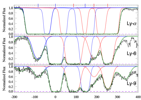
Figure 8: Lyman series absorption for the $z\sim 2.45$ LLS towards Q1549+1919. The three absorbers shown in red have their $N_{\rm HI}$ fixed to the values presented in the appendix of R13 for this LLS. R13 do not provide exact redshifts or velocity widths for these absorbers, so they have been chosen to best match by eye the absorption presented in R13 while still presenting a good overall absorption model to the LLS. In addition, we show in blue all additional absorbers with $\log N_{\rm HI}>15.0$ that are needed to fit the strongest absorption features in the LLS. The green curve shows the full absorption model, which includes additional $\log N_{\rm HI}<15.0$ absorbers to provide a good fit to the data. In total, six absorbers, including three with $\log N_{\rm HI}>16.5$.

The concept of line-blending is nicely illustrated by the R13 data. For example. consider the absorption complex at $z\sim 2.45$ toward Q1549+1919. Analysis of the full Lyman series reveals a complex system of six absorbers having $N_{\rm HI}>10^{15}\,{\rm cm^{-2}}$, all within $\Delta v=400{\rm km~{}s^{-1}}$. These lines have individual column densities, in increasing strength, of $N_{\rm HI}=10^{15.79},10^{15.85},10^{16.32},10^{16.70},10^{16.82}$ and $10^{17.00}\,{\rm cm^{-2}}$. Although there are significant degeneracies between components in the model, one thing is certain: multiple strong ($N_{\rm HI}>10^{15.5}\,{\rm cm^{-2}}$) H I absorbers are required to account for the observed absorption (Figure 8). If assessed independently via Lyman continuum opacity, the complex would be recorded as an LLS with $N_{\rm HI}=10^{17.4}\,{\rm cm^{-2}}$ and would additionally contribute to $f(N_{\rm HI})$ at this higher $N_{\rm HI}$ value. We conclude that R13 underestimated $\lambda_{\rm mfp}^{912}$ because of the double counting of LL opacity; indeed, this is also true of all previous authors that coupled $f(N_{\rm HI})$ and LLS statistics. We note further that line-blending may have also impacted the $f(N_{\rm HI})$ model of O13, who reported a deficit of $N_{\rm HI}\approx 10^{17}\,{\rm cm^{-2}}$ systems relative to R13. The O13 conclusion was based on their $\lambda_{\rm mfp}^{912}$ value and the incidence of LLS. As such, clusters of $N_{\rm HI}=10^{16}\,{\rm cm^{-2}}$ lines were included as LLS and fewer such systems were required to match the $\lambda_{\rm mfp}^{912}$ measurement.

Second (and similarly), the clustering of absorption systems means optically thick gas is not randomly distributed throughout the universe. This contradicts the standard formalism (Equation 1) used to calculate $\tau_{\rm eff,LL}$ which assumes a Poisson distribution in the IGM. For accurate results, one must fully account for clustering to use $f(N_{\rm HI})$ as a description of the IGM. A full and proper treatment must await future observations, in tandem with the analysis of cosmological simulations that include hydrodynamics and radiative transfer. For now, we offer below some insight on how the clustering of LLS will tend to increase the $\lambda_{\rm mfp}^{912}$.

3.3 Modifying the Opacity of the IGM for the Clustering of LLS

Equation 1 for the effective continuum optical depth of a clumpy IGM is valid under the assumption of a random distribution of absorbers along the line of sight. The formula can be easily understood if we consider a situation in Euclidean space in which all absorbers have the same optical depth $\tau_{0}$, and the mean number of systems along the path is $\bar{N}$. In this case the Poissonian probability of encountering a total optical depth $N\tau_{0}$ along the path (with $N$ integer) is $p(N)$, where

$$p(N)=e^{-\bar{N}}{{\bar{N}}^{N}\over N!}.$$ (3)

The mean attenuation is then

$$\langle e^{-\tau}\rangle = \sum\limits_{N=0}^{\infty}e^{-N\tau_{0}}p(N)=e^{-\bar{N}}\sum\limits_{N=0}^{\infty}{(e^{-\tau_{0}}{\bar{N}})^{N}\over N!}$$ (4)

$$= e^{-{\bar{N}}(1-e^{-\tau_{0}})},$$

and the effective optical depth is $\tau_{\rm eff}=-\ln\langle e^{-\tau}\rangle={\bar{N}}(1-e^{-\tau_{0}})$ (cf. Equation 1). When $\tau_{0}\ll 1$, $\tau_{\rm eff}$ becomes equal to the mean optical depth. In the opposite limit, the obscuration is picket-fence, and the effective optical depth becomes equal to the mean number of optically thick absorbers along the line of sight.

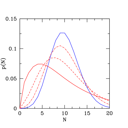
Figure 9: The frequency distribution $p(N)$ for $\bar{N}=10$ and $N=0,1,2,3,...$. The Poisson limit is shown with the blue solid curve, while the highly clustered distributions for $b=0.2,0.4,0.6$ are shown with the red dot-dashed, dashed, and solid curves, respectively.

In the evaluation of Equation 1, then lines cluster together it is the total $N_{\rm HI}$ that contributes. To assess the impact of gravitational clustering on the effective opacity and therefore on the mean free path of ionizing radiation through the IGM, let us assume instead a probability distribution function of the form

$$p(N)={{\bar{N}}(1-b)\over N!}[{\bar{N}}(1-b)+Nb]^{N-1}e^{-{\bar{N}}(1-b)-Nb}.$$ (5)

Predicted by gravitational thermodynamics to describe galaxy clustering in an expanding universe (Saslaw & Hamilton, 1984; Saslaw, 1989), this function reduces to a Poisson distribution (no gravitational interactions) when the parameter $b=-W/2K$, which measures the degree of virialization, is $b=0$. Figure 9 depicts the frequency distribution $p(N)$ for $\bar{N}=10$ and $b=0$ (Poisson), 0.2, 0.4, and 0.6. The extreme non-Poisson limit corresponds to $b\rightarrow 1$, while the first moment of the distribution, $\langle(\Delta N)^{2}\rangle^{1/2}\equiv\langle(N-{\bar{N}})^{2}\rangle^{1/2}=\sqrt{N}/(1-b)$ shows that correlated fluctuations are amplified over the Poisson value by the factor $(1-b)^{-1}$.

At a fixed $\bar{N}$, the clustering of absorption systems decreases the opacity of the IGM compared to a random distribution, when viewed from a random position. This is shown in Figure 10, where we have used the probability function in Equation (5) to compute the effective optical depth (in Euclidean space) for optically thick absorbers ($\tau_{0}=1$) at varying ${\bar{N}}$ and clustering parameter $b$. This toy model shows how even moderate clustering ($b=0.2-0.4$) could result in a reduction of the effective absorption opacity of 15-45%, greatly easing the tension between the directly measured “true” MFP and the one incorrectly inferred from $f(N_{\rm HI})$ under the assumption of a randomly distributed population of thick absorbers.

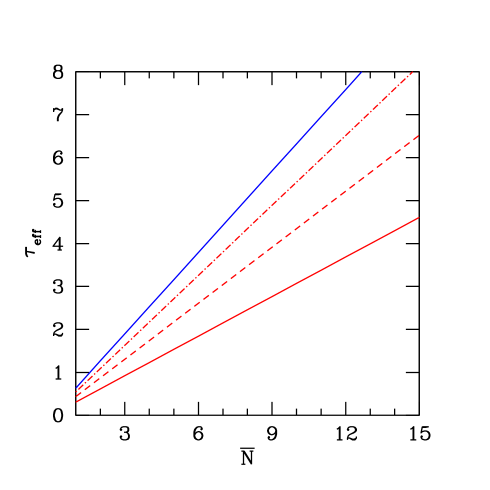
Figure 10: The effective opacity in Euclidean space corresponding to the frequency distribution of equation (5), as a function of the mean number of absorbers $\bar{N}$. Individual absorbers have optical depth $\tau_{0}=1$. As in Figure 9, the Poisson limit is shown with the blue solid curve, while the highly clustered distributions for $b=0.2,0.4,0.6$ are shown with the red dot-dashed, dashed, and solid curves, respectively.

4 Summary and Future Work

In this manuscript, we have examined the principal observational constraints on characterizing the H I opacity of the IGM. We studied the tension between estimations of the mean free path $\lambda_{\rm mfp}^{912}$ (Figures 1,3; O13, R13), and emphasized that current measurements of $f(N_{\rm HI})$ at $N_{\rm HI}\approx 10^{15}-10^{17}\,{\rm cm^{-2}}$ are in strong conflict (Figure 5; R13, K13). While some of these disagreements may be the result of statistical variance, we argued that they result primarily from two effects related to the clustering of strong absorption-line systems.

The first effect is known as line-blending, the presence of two or more absorption systems with comparable $N_{\rm HI}$ at small velocity separation. Although line-blending has previously been recognized, its impact on measurements of $f(N_{\rm HI})$ and $\lambda_{\rm mfp}^{912}$ have been under appreciated. Going forward, it will be necessary to define $f(N_{\rm HI})$ within well-defined velocity windows. In particular, attempts to combine $f(N_{\rm HI})$ measurements from line-profile fitting with the observed incidence of LLS have led to the double counting of Lyman limit opacity. Specifically, to combine surveys of the LLS with measurements of $f(N_{\rm HI})$ from line-profile fitting one must ‘smooth’ the latter by a velocity window $\Delta v$. Current LLS surveys based on lower resolution spectra require $\Delta v\approx 2000{\rm km~{}s^{-1}}$ (Prochaska et al., 2010). The size of $\Delta v$ may only be minimized through surveys at very high spectral resolution and S/N covering the full Lyman series (e.g. the ESO X-Shooter Large Program; PI: Lopez).

The other effect, the large-scale clustering of absorption systems, will likely require calibration from cosmological simulations using radiative transfer. It is also possible that one may introduce a clustering formalism akin to the halo occupation distribution function for galaxies (Tinker & Chen, 2008). Indeed, Zhu et al. (2013) have presented evidence for two terms for the clustering of Mg II systems around luminous red galaxies, but the clustering of LLS is well modeled by a single power-law (Prochaska et al., 2013). To date, the LLS have been correlated with luminous, $z\sim 2$ quasars (Hennawi & Prochaska, 2007; Prochaska et al., 2013). Further studies should examine the auto-correlation function (Fumagalli et al., 2013a) as well as the cross-correlation function with the quasi-linear Ly$\alpha$ forest. And, ultimately, one must modify the definition for the effective opacity of the IGM, possibly in a manner similar to the toy model of $\S$ 3.3.

Returning to the MFP, there is yet another aspect of clustering which may influence this measurement and one’s estimate for the intensity of the EUVB: the absorption systems are clustered around the ionizing sources (quasars, galaxies). Prochaska et al. (2013) demonstrated that quasars are strongly clustered to optically thick gas, exhibiting a covering fraction $f_{C}$ that approaches unity as one tends to small impact parameters transverse to the sightline. Extrapolating their results to zero impact parameter (i.e. along the sightline or ‘down-the-barrel’), one recovers $f_{C}>0.8$. This suggests that the ionizing radiation field from quasars could be strongly attenuated. One observes, however, that very few quasars exhibit strong LL opacity at $z\approx z_{\rm em}$ (Prochaska et al., 2010). In fact, Prochaska et al. (2010) measured a deficit of LLS within $\delta v=3000{\rm km~{}s^{-1}}$ of $z\sim 3.7$ quasars relative to the incidence measured at large velocity separations along the same sightlines. The natural interpretation is that quasars photoionize the gas along the sightline, to distances of tens of Mpc (e.g. Hennawi & Prochaska, 2007). This quasar proximity effect may further increase $\lambda_{\rm mfp}^{912}$ and the resultant metagalactic flux. We encourage large volume simulations to explore these effects.

Of course, galaxies may also contribute to the EUVB, especially at redshifts $z>4$ where one observes a steep decline in the comoving number density of bright quasars (Fan et al., 2006). Similar to the quasar-LLS clustering, Rudie et al. (2012) have reported on an excess of strong H I absorption systems in the environment of Lyman break galaxies (LBGs). R13 further posited that the MFP from LBGs will be smaller due to such clustering, although those authors ignored any proximity effect associated to the LBG radiation field. One can test these effects by generating a composite spectrum in the LBG rest-frame, akin to our quasar analysis. We expect the data already exist and encourage such analysis.

References

- Altay et al. (2013) Altay, G., Theuns, T., Schaye, J., Booth, C. M., & Dalla Vecchia, C. 2013, Monthly Noticies of the Royal Astronomical Society
- Bahcall & Peebles (1969) Bahcall, J. N., & Peebles, P. J. E. 1969, Astrophysical Journal Letters, 156, L7+
- Becker & Bolton (2013) Becker, G. D., & Bolton, J. S. 2013, ArXiv e-prints
- Becker et al. (2013) Becker, G. D., Hewett, P. C., Worseck, G., & Prochaska, J. X. 2013, Monthly Noticies of the Royal Astronomical Society, 430, 2067
- Bergeron et al. (2004) Bergeron, J., et al. 2004, The Messenger, 118, 40
- Compostella et al. (2013) Compostella, M., Cantalupo, S., & Porciani, C. 2013, Monthly Noticies of the Royal Astronomical Society
- Croft et al. (2002) Croft, R. A. C., Weinberg, D. H., Bolte, M., Burles, S., Hernquist, L., Katz, N., Kirkman, D., & Tytler, D. 2002, Astrophysical Journal, 581, 20
- Dixon et al. (2013) Dixon, K. L., Furlanetto, S. R., & Mesinger, A. 2013, ArXiv e-prints
- Fan et al. (2006) Fan, X., Carilli, C. L., & Keating, B. 2006, Annual Review of Astronomy & Astrophysics, 44, 415
- Faucher-Giguère et al. (2008a) Faucher-Giguère, C.-A., Lidz, A., Hernquist, L., & Zaldarriaga, M. 2008a, Astrophysical Journal, 688, 85
- Faucher-Giguère et al. (2008b) Faucher-Giguère, C.-A., Prochaska, J. X., Lidz, A., Hernquist, L., & Zaldarriaga, M. 2008b, Astrophysical Journal, 681, 831
- Fritsch & Carlson (1980) Fritsch, F. N., & Carlson, R. E. 1980, SIAM Journal on Numerical Analysis, 17, 238
- Fumagalli et al. (2013a) Fumagalli, M., Hennawi, J. F., Prochaska, J. X., Kasen, D., Dekel, A., Ceverino, D., & Primack, J. 2013a, ArXiv e-prints
- Fumagalli et al. (2013b) Fumagalli, M., O’Meara, J. M., Prochaska, J. X., & Worseck, G. 2013b, Astrophysical Journal, 775, 78
- Fumagalli et al. (2011) Fumagalli, M., Prochaska, J. X., Kasen, D., Dekel, A., Ceverino, D., & Primack, J. R. 2011, Monthly Noticies of the Royal Astronomical Society, 418, 1796
- Haardt & Madau (1996) Haardt, F., & Madau, P. 1996, Astrophysical Journal, 461, 20
- Haardt & Madau (2012) —. 2012, Astrophysical Journal, 746, 125
- Hennawi & Prochaska (2007) Hennawi, J. F., & Prochaska, J. X. 2007, Astrophysical Journal, 655, 735
- Kim et al. (2001) Kim, T., Cristiani, S., & D’Odorico, S. 2001, Astronomy & Astrophysics, 373, 757
- Kim et al. (2002) Kim, T.-S., Carswell, R. F., Cristiani, S., D’Odorico, S., & Giallongo, E. 2002, Monthly Noticies of the Royal Astronomical Society, 335, 555
- Kim et al. (2013) Kim, T.-S., Partl, A. M., Carswell, R. F., & Müller, V. 2013, Astronomy & Astrophysics, 552, A77
- Kirkman & Tytler (1997) Kirkman, D., & Tytler, D. 1997, Astrophysical Journal, 484, 672
- Kirkman et al. (2005) Kirkman, D., et al. 2005, Monthly Noticies of the Royal Astronomical Society, 360, 1373
- Lee et al. (2013) Lee, K.-G., et al. 2013, Astronomical Journal, 145, 69
- Lusso et al. (2013) Lusso, E., et al. 2013, ArXiv e-prints
- McDonald et al. (2005) McDonald, P., et al. 2005, Astrophysical Journal, 635, 761
- McQuinn et al. (2011) McQuinn, M., Oh, S. P., & Faucher-Giguère, C.-A. 2011, Astrophysical Journal, 743, 82
- Meiksin & Madau (1993) Meiksin, A., & Madau, P. 1993, Astrophysical Journal, 412, 34
- Nestor et al. (2013) Nestor, D. B., Shapley, A. E., Kornei, K. A., Steidel, C. C., & Siana, B. 2013, Astrophysical Journal, 765, 47
- Noterdaeme et al. (2012) Noterdaeme, P., et al. 2012, Astronomy & Astrophysics, 547, L1
- Noterdaeme et al. (2009) Noterdaeme, P., Petitjean, P., Ledoux, C., & Srianand, R. 2009, Astronomy & Astrophysics, 505, 1087
- O’Meara et al. (2007) O’Meara, J. M., Prochaska, J. X., Burles, S., Prochter, G., Bernstein, R. A., & Burgess, K. M. 2007, Astrophysical Journal, 656, 666
- O’Meara et al. (2013) O’Meara, J. M., Prochaska, J. X., Worseck, G., Chen, H.-W., & Madau, P. 2013, Astrophysical Journal, 765, 137
- Palanque-Delabrouille et al. (2013) Palanque-Delabrouille, N., et al. 2013, ArXiv e-prints
- Pâris et al. (2012) Pâris, I., et al. 2012, Astronomy & Astrophysics, 548, A66
- Prochaska et al. (2013) Prochaska, J. X., et al. 2013, ArXiv e-prints
- Prochaska et al. (2005) Prochaska, J. X., Herbert-Fort, S., & Wolfe, A. M. 2005, Astrophysical Journal, 635, 123
- Prochaska et al. (2010) Prochaska, J. X., O’Meara, J. M., & Worseck, G. 2010, Astrophysical Journal, 718, 392
- Prochaska & Wolfe (2009) Prochaska, J. X., & Wolfe, A. M. 2009, Astrophysical Journal, 696, 1543
- Prochaska et al. (2009) Prochaska, J. X., Worseck, G., & O’Meara, J. M. 2009, Astrophysical Journal Letters, 705, L113
- Ribaudo et al. (2011) Ribaudo, J., Lehner, N., & Howk, J. C. 2011, Astrophysical Journal, 736, 42
- Rudie et al. (2013) Rudie, G. C., Steidel, C. C., Shapley, A. E., & Pettini, M. 2013, Astrophysical Journal, 769, 146
- Rudie et al. (2012) Rudie, G. C., et al. 2012, Astrophysical Journal, 750, 67
- Saslaw (1989) Saslaw, W. C. 1989, Astrophysical Journal, 341, 588
- Saslaw & Hamilton (1984) Saslaw, W. C., & Hamilton, A. J. S. 1984, Astrophysical Journal, 276, 13
- Schneider et al. (2010) Schneider, D. P., et al. 2010, Astronomical Journal, 139, 2360
- Slosar et al. (2013) Slosar, A., et al. 2013, Journal of Cosmology and Astroparticle Physics, 4, 26
- Songaila & Cowie (2010) Songaila, A., & Cowie, L. L. 2010, Astrophysical Journal, 721, 1448
- Telfer et al. (2002) Telfer, R. C., Zheng, W., Kriss, G. A., & Davidsen, A. F. 2002, Astrophysical Journal, 565, 773
- Tinker & Chen (2008) Tinker, J. L., & Chen, H.-W. 2008, Astrophysical Journal, 679, 1218
- Viel et al. (2009) Viel, M., Bolton, J. S., & Haehnelt, M. G. 2009, Monthly Noticies of the Royal Astronomical Society, 399, L39
- White et al. (2012) White, M., et al. 2012, Monthly Noticies of the Royal Astronomical Society, 424, 933
- Worseck & Others (2013) Worseck, G., & Others, A. 2013, in prep