On Self-Avoiding Walks across n-Dimensional Dice
and Combinatorial Optimization: An Introduction

Abstract –  Self-avoiding walks (SAWs) were introduced in chemistry to model the real-life behavior of chain-like entities such as solvents and polymers, whose physical volume prohibits multiple occupation of the same spatial point. In mathematics, a SAW lives in the n-dimensional lattice $\mathbb{Z}^{n}$ which consists of the points in $\mathbb{R}^{n}$ whose components are integers.

In this paper, SAWs are a metaphor for walks across faces of $n$-dimensional dice, or more formally, a hyperhedron family ${\cal H}(\Theta,b,n)$. Each face is assigned a label {${\underline{\varsigma}}:\Theta({\underline{\varsigma}})$}; ${\underline{\varsigma}}$ represents a unique $n$-dimensional coordinate string ${\underline{\varsigma}}$,  $\Theta({\underline{\varsigma}})$ is the value of the function $\Theta$ for ${\underline{\varsigma}}$. The walk searches $\Theta({\underline{\varsigma}})$ for optima by following five simple rules: (1) select a random coordinate and mark it as the ‘initial pivot’; (2) probe all unmarked adjacent coordinates, then select and mark the coordinate with the ’best value’ as the new pivot; (3) continue the walk until either the ’best value’ <= ‘target value’ or the walk is being blocked by adjacent coordinates that are already pivots; (4) if the walk is blocked, restart the walk from a randomly selected ‘new initial pivot’; (5) if needed, manage the memory overflow with a streaming-like buffer of appropriate size. Hard instances from a number of problem domains, including the 2D protein folding problem, with up to $(2^{25})*(3^{24})$ coordinates, have been solved with SAWs in less than 1,000,000 steps – while also exceeding the quality of best known solutions to date.

I.   Introduction

Instances of combinatorial problems arise in many contexts such as operations research, computer-aided design, machine learning, robotics, data mining, bioinformatics, etc. An exhaustive search for an optimum solution is not possible for most instances of practical size due to the huge number of feasible solutions. The question arises about the choice of heuristic algorithms to be deployed by the solver. To date, stochastic search methods offer the best compromise, including Metropolis-Hastings algorithm [1, 2], simulated annealing [3, 4], Gibbs sampling [5], tabu search [6, 7], and many others. New heuristics are emerging on Wikipedia and in journals under metaphors such as ant colonies, bird flocks, natural disasters, biological processes, etc.

Our approach is simple; we only take a few liberties with rigorous mathematical notation. When we refer to a function $f(x_{1}^{i},x_{2}^{i},\ldots x_{n}^{i})$, we imply an objective function, which in general is a multivalued function, returning a value for a specific coordinate $(x_{1}^{i},x_{2}^{i},\ldots x_{n}^{i})$. The support set of the function is defined in terms of such coordinates. A combinatorial problem is defined by its function and its coordinate type. Coordinates are represented as a set of strings, such as $01011...$ for a binary coordinate, $210210...$ for a ternary coordinate, $4,2,5,3,...$ for a permutation coordinate, etc. A combinatorial problem can also be stated in terms of concatenated coordinates of different types. For example, we define the 2D protein folding problem on a square lattice by computing its function values with coordinates represented as a concatenation of binary and ternary coordinates.

We define a walk as a sequence of steps that chain a set of pivot coordinates, adjacent coordinates as the local neighborhood of the pivot coordinate, and probing as evaluating the function for values in this neighborhood. A feasible solution of the combinatorial problem is a pair (coordinatePivot:valuePivot). Once we capture the description of the combinatorial problem in these terms, the search procedure is as simple and as generic as the five rules outlined in the abstract – for any combinatorial problem. For more about this notation and examples of various problem instances, see [8].

We have a number of on-going projects with the goal to prototype SAWs as a powerful general-purpose search procedure that, unlike alternatives, does not require knobs and dials to set-up. These projects include instances of problems defined for Golomb rulers, integer partitioning, maximum independent set, minimum vertex cover and maximum clique, graph linear arrangement, job scheduling, etc. A nearly completed project demonstrates significant improvements in solutions of the notoriously hard labs problem [9]: here we compare, side-by-side, the performance of state-of-the-art memetic/tabu and SAW solvers. In the present paper we apply SAW to solve the 2D protein folding problem on a square lattice [10]. Since this implementation is based on a scripting language, it is not suitable for solving very large problems. However, the solver does achieve a number of state-of-the art solutions on a significant subset of problem instances from the literature and an asymptotic performance that may well dominate alternative solvers when fully implemented.

The paper is organized as follows. To motivate the approach taken in this paper, Section II starts with a fable about Gretel and Hansel who devise distinctive methods to search for a pass-key. Section III formulates the problem and concludes with pseudo code, describing global search with self-avoiding walk. Section IV summarizes a number of performance experiments in 2D protein folding problem defined on a square lattice. With some 1000 independent solutions for each member of 10 instance classes of increasing size (with at least 3 instances in each class), these experiments not only replicate the earlier work of others, but also reveal new and improved folding conformations. The paper concludes with directions for future work.

II.   Motivation

We introduce a fable to motivate our approach. It involves Gretel and Hansel, living in two adjacent apartments, and a Joker whose omnipresence is never revealed directly. Gretel and Hansel are returning from a party. They discover not only that locks have been changed on both apartment doors with punch-key locks but also that mats that hid the keys were replaced with two urns, each containing a set 36 tickets. Each ticket has a printed label with five digits in the format xx.yy:z; only one label opens Gretel’s door, and only one opens Hansel’s door. The two sets are identical.

Who gets in first? Watching Gretel, she takes the ticket from the urn and if she does not succeed in opening the door, she puts the ticket into her handbag and retrieves another ticket. Hansel, who had a few drinks at the party, takes the ticket and if he does not succeed in opening the door, returns the ticket to the urn. We say that Gretel is sampling contents of the urn without replacement, while Hansel is sampling with replacement. The probability of Gretel finding the correct ticket on trial $k$ follows uniform distribution, given $n$ tickets: the probability is $1/n$, the mean value is $(n+1)/2$, and the variance is $(n^{2}-1)/12$. However, the probability of Hansel finding the correct ticket on trial $k$ follows geometric distribution: the probability is $(1/n)(1-(1/n))^{k-1}$, the mean value is $n$, and the variance is $n^{2}(1-(1/n))$. The point of the fable so far: we learn that in a search scenarios such as described here, one can improve the chance of first success by dynamically reducing the search space after each trial. In the best case for Gretel, the capacity of her handbag must match the capacity of the urn. If the capacity of the handbag is less than the capacity of the urn, and the handbag gets full before finding the key, she needs to return the unsuccessful ticket to the urn before proceeding with the next trial. In the average case, Gretel’s search, even with handbag of limited capacity, always requires fewer trials than Hansel’s.

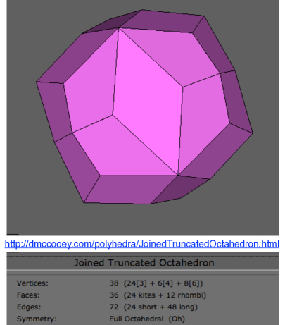
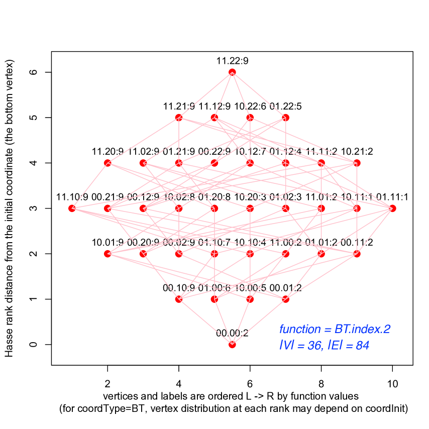
The item on the left is a polyhedron with 36 faces and 72 edges [11]. Each face has 4 adjoining faces. This polyhedron is an approximation of the a virtual combinatorial object, a hyperhedron introduced next. By assigning to each face a unique coordinate as a concatenation of a binary strings of length 2 and a ternary string of length 2, we create a hyperhedron with $2^{2}\times 3^{2}=36$ faces, the same as polyhedron. However, this hyperhedron has 84 edges compared to 72 in the polyhedron. We count the edges by creating a Hasse graph [8]: each face is assigned a vertex with a unique label and the edges between vertices represent adjacencies between faces. We find that the number of edges between vertices varies from 4 to 6. The label always contains a unique coordinate string, and in most cases, the label is extended with a value returned by the function evaluated with the coordinate. The Hasse graph is drawn as an undirected layered graph on a grid such as the one below: it has 36 vertices and 84 edges with labels such as 00:00:2, 00.10:9, and 01:21:9; the string following ’:’ represents the value. We say that vertices 00.00:2 and 00.10:9 are adjacent since the distance between coordinates is 1, while coordinates 00.10:9 and 01:21:9 are not adjacent since the distance is 3.

Figure 1: A polyhedron solid and a hyperhedron projection: each has 36 faces, but face-to-face adjacencies are different.

Another surprise awaits after Gretel and Hansel manage to make an entry. Neither has stepped into their apartment’s vestibule; instead, each is now standing on a four-sided platform (in their own apartment) and can see, besides the platform on which they are standing, only the surfaces of the four adjacent platforms sloping downwards. Each of them believes that she/he is standing on a face of a huge platonic solid, such as the polyhedron with 36 faces and 72 edges between the faces shown in in Figure 1. Neither realizes that they stepped into a virtual world where not everything is as it seems. The face on which they are standing belongs to a virtual combinatorial object hyperhedron, also with 36 faces, but as they will walk from face to face, they will discover that some faces have five adjacent faces, some have even six.

Figure 2: A Hamiltonian walk in the Hasse graph taken by Gretel and a self-avoiding walk taken Hansel. Vertices traversed during the walk are in two categories: (1) only binary coordinate is changing, ternary coordinate is fixed; (2) binary coordinate is fixed, only ternary coordinate is changing. At each pivot, before Hansel decides on the next step, he probes the function values at all adjacent coordinates (that are not yet pivots in the walk) and chooses the coordinate with ’valueBest’. If there are multiple adjacent coordinates with the same ’valueBest’, the choice is random. Gretel’s walk, self-avoiding by definition, continues until ’valueBest = valueTarget = 1’ and the key found fits her lock, Hansel’s walk terminates when the key found fits his lock.

Joker has replaced the two urns with two hyperhedrons and pasted the tickets from each urn into the center of the face in each the hyperhedron, with labels showing. He also hid Gretel’s pass-key under one ticket, and Hansel’s key under another ticket.

Only Joker has the global view of the hyperhedron. He interprets it as follows. He moves inside the hyperhedron, finds the center of the face, and attaches one end of a string to the center and attaches the other string to the center of the adjacent face. He repeats the process for all faces and thus creates a graph; a graph with 36 face-centered vertices and 84 edges. To represent this graph in the plane, he defines a distance between the coordinates assigned to each label and makes a projection of the graph as a layered graph shown in the bottom of Figure 1. This graph is not visible to Gretel and Hansel, however, the graph enables Joker to trace each step they would make during their search. Joker also assigned function values to each coordinate: his choice of values is expected to confound Gretel and Hansel in their search. He gives both one, and only one, hint about the pass-key: the ticket most likely hiding the pass-key is the one where value on the label is 1 or less than 1. If Gretel find Hansel’s key first, the key would not fit and she needs to continue the search – and vice versa for Hansel.

Who will find the pass-key to the apartment first? Each is standing on the face with the label 00.00:2 (at the bottom of Figure 1). From this face, Gretel and Hansel can see only the four adjacent faces: 00.10:9, 01.00:6, 10.00:5, 00.01:2. Their task is to walk from face to face until they find the pass-key to their old apartment.

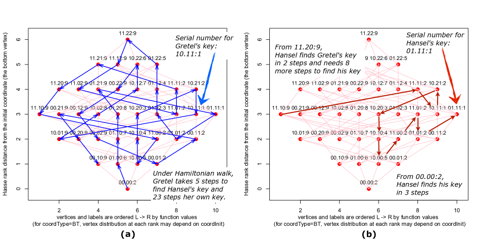
Gretel is a computer science major and remembers a lecture about Hamiltonian walks in graphs. She knows that she is standing on one of 36 faces and that if she associates each face with a vertex in a graph and the edges between adjacent faces with edges in this graph, she can compute and remember the path that visits each face only once. In the worst case, she will take 35 steps to find the key. The procedure she uses to compute the coordinates for each step in the Hamiltonian walk is not as simple to explain as the procedure used by Hansel and explained next. Suffice it to say that function values associated with each coordinate have no role in determining the Hamiltonian path in the graph. An example of Gretel’s walk, as traced by Joker, is shown in 2-a. She takes 5 steps to find Hansel’s key and needs to continue for a total of 23 steps before finding her key. The first step, from 00.00:2 to 00.00:6, is a deliberate step in this Hamiltonian walk – a step that Hansel would never have taken from this starting position, for reasons we explain next.

Hansel’s major is land surveying and he takes the hint about function values associated with each coordinate very seriously. He devises a few rules before starting the walk: (1) mark the face from where the walk starts with an easy-to-spot token; later on in the paper, we call this face the initial pivot. (2) probe each adjacent face that has not yet been marked and write its value on a list. (3) select the adjacent face with the smallest value, step on this face, call it a current pivot, and mark it with a new token. If there are several faces with the same value, make a random selection. (4) repeat step (2) from the current pivot until reaching the target value. The process of marking the pivots during the walk with tokens makes this walk self-avoiding. Hansel can run into a problem with these rules in two cases: (1) he runs out of tokens and can no longer mark the walk; (2) he steps onto a face where all adjacent faces have been marked already, i.e. the walk is trapped. In either of these cases, Hansel has to collect all tokens and restart the walk from a new face, now selected by a random jump. An example of Hansel’s walk, as traced by Joker, is shown in Figure 2-b. While Hansel can find the ticket that hides his pass-key in 3 steps or less from many initial positions, it takes 10 steps to find his key if he starts from 10.10:9 and takes the third step to 10.21:2 instead of 00.11:2 (both of these choice are equally likely).

What have we learned from the second part of the fable is this: (1) A Hamiltonian walk, while self-avoiding by definition, should not be the first choice under the search scenarios described in this paper. Moreover, the approach would not scale to large problem instances. (2) On the other hand, rules devised by Hansel seem to be highly effective. The good news is that these rules are now enabling effective combinatorial searches not only in the cases of protein folding investigated in this paper but also on hard combinatorial problems in other domains, notably the low autocorrelation binary sequence problem, where the self-avoiding walks solve large problems that could not be solved with state-of-the art memetic/tabu search methods [9]. Moreover, problem of self-avoiding walks getting trapped has not presented itself neither in the case of protein folding nor the case of the labs problem [9].

We used to call these walks Hansel’s walks until we learned about polymer and protein chain folding and self-avoiding walks [12]. In our context, the self-avoiding walks are walks in hyperhedra, a virtual world, not in a space of real-world constraints imposed by various lattice formulations in two or three dimensions [13]. In our formulation we deal with real-world folding constraints by way of computing the function values in terms of our coordinate system which foremost defines positions and distances between face-centered vertices in hyperhedra. For problems such as protein folding, some coordinates may induce a penalty value when a conflict is detected during folding; the penalty value assigned may depend on the perceived level of conflict. Hansel’s strategy, of always selecting the best available value in the local neighborhood for the next step, keeps the walk going, across faces of a specific hyperhedron, for as long as required.

III.   Notation and Definitions

Self-avoiding walks (SAWs) were first introduced by the chemist Paul Flory in order to model the real-life behavior of chain-like entities such as solvents and polymers, whose physical volume prohibits multiple occupation of the same spatial point [12]. In mathematics, a SAW lives in the n-dimensional lattice $\mathbb{Z}^{n}$ which consists of the points in $\mathbb{R}^{n}$ whose components are all integers [14].

In Section II, we illustrated a grid of a finite dimension that was created by projecting face-centered vertices in a hyperhedron, onto a plane as a Hasse graph. This section illustrates: (1) projections of vertices in Hasse graphs that have 1-to-1 relationship to lattices defined by unit cells; (2) example of a SAW-in-a-hyperhedron search for best folding of a protein chain of size $n$ on a specific 2D lattice ; (3) formalized definitions of walks and a generic SAW pseudo-code as a principal component of a global stochastic search solver.

Lattices, unit cells, and graphs. A lattice is a periodic array of points on a grid in space. A unit cell is a subset of $|V|$ points on a grid in a lattice [15]. A self-avoiding walk in a unit cell and a Hamiltonian walk in a Hasse graph with $|V|$ vertices [8] can be considered as two faces of the same coin. We illustrate this premise with the three examples in Figure 3. In Figure 3-a on the left, the primitive cell is a square, forming a unit cell of 9 squares with 16 grid points. On the right, we have a Hasse graph with 16 vertices with binary coordinate labels; this graph is regular since the degree of each vertex is 4 – i.e. each vertex has 4 immediate neighbors. Given the starting point in the unit cell, we can express the walk in terms of directional encoding (North, South, East, West): for the first six steps we would write NWSSSE. Given the starting point in the graph, we express the walk as a sequence of its pivot coordinates (2): 0110, 0111, 0101, 0100, … etc. However, there is a significant difference in the two data structures: in the unit cell, neighborhood size, depending on the location in the grid, varies from 2, 3, to 4, whereas in the graph, each vertex has 4 neighbors.

Figure 3: Two sides of the same coin: instances of three self-avoiding walks of lengths $2^{4}-1$, $4^{2}-1$, and $3^{3}-1$ in 2-D and 3-D in unit cells, subsets of points on a grid in a lattice [15], versus instances of three Hamiltonian walks of the same length in Hasse graphs [8] defined by dimensions 4 (wrt to base 2), 2 (wrt to base 4), and 3 (wrt to base 3). The walks in unit cells are contiguous only with respect to coordinates defined in lattices. Similarly, the walks in Hasse graphs are contiguous only with respect to coordinates defined in Hasse graphs.

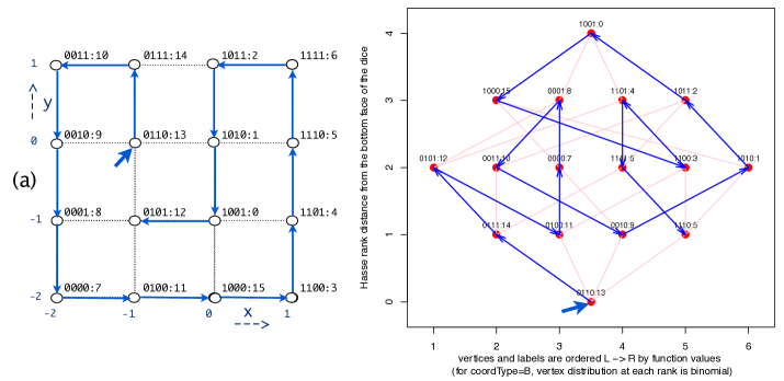
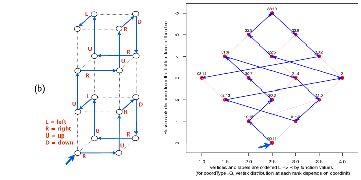
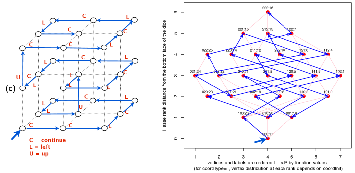
The crux in drawing the Hasse graph into its distinct layers is the notion of Hasse rank distance between the vertices with respect to the reference vertex (or the origin vertex) placed at the very bottom of the graph [8]. When coordinates are binary strings, the rank distance is the familiar Hamming distance, for coordinate that represent permutations, the rank distance is the permutation inversion distance, the rank distance between the ternary and quaternary coordinates in Figure 3 is defined as an arithmetic addition of modulo-3 or modulo-4 distances between coordinate components. For example, the distance between 2101 and 0201 is 2+1+0+0=3, the distance between 3210 and 0123 is 3+1+1+3=8, etc. The distance between two coordinates that have been concatenated, shown in the Hasse graph in Figure 1, is an arithmetic addition of distances between the corresponding concatenated segments, for example the distance between 00.10 and 01.21 is (0+1)+(1+1)=3.

Function values assigned to coordinates in Figure 3 are shown for completeness. They represent a special case of index function related to each coordinate. Typically, they exhibit 1, 2, or 4 minima and have been designed for performance testing of combinatorial algorithms [8]. However, these values have no particular significance in Figure 3 .

In Figure 3-b on the left, the primitive cell is a cube, forming a unit cell as a stack of 3 cubes with 16 grid points. On the right, we have a Hasse graph with 16 vertices with quarternary coordinate labels; this graph is not regular since the degree of each vertex varies from 2, 3, to 4. In Figure 3-c on the left, the primitive cell is a cube, forming a unit cell as a large cube that contains 8 primitive cubes with 27 grid points. On the right, we have a Hasse graph with 27 vertices with ternary coordinate labels; this graph is not regular since the degree of each vertex varies from 3, 4, 5, to 6.

In the context of this paper, it is important to also study advances in self-avoiding walks being made in physics and elsewhere, for example on the progression of improvements in the walk lengths of self-avoiding walks on 2-, 3-, and 4-dimensional lattices [16].

Protein folding examples. There are numerous articles that cover many more details about protein folding than we can present here, from very technical [10] to tutorial [17]. Our presentation attempts to be generic and aims to make the problem accessible as a complex puzzle.

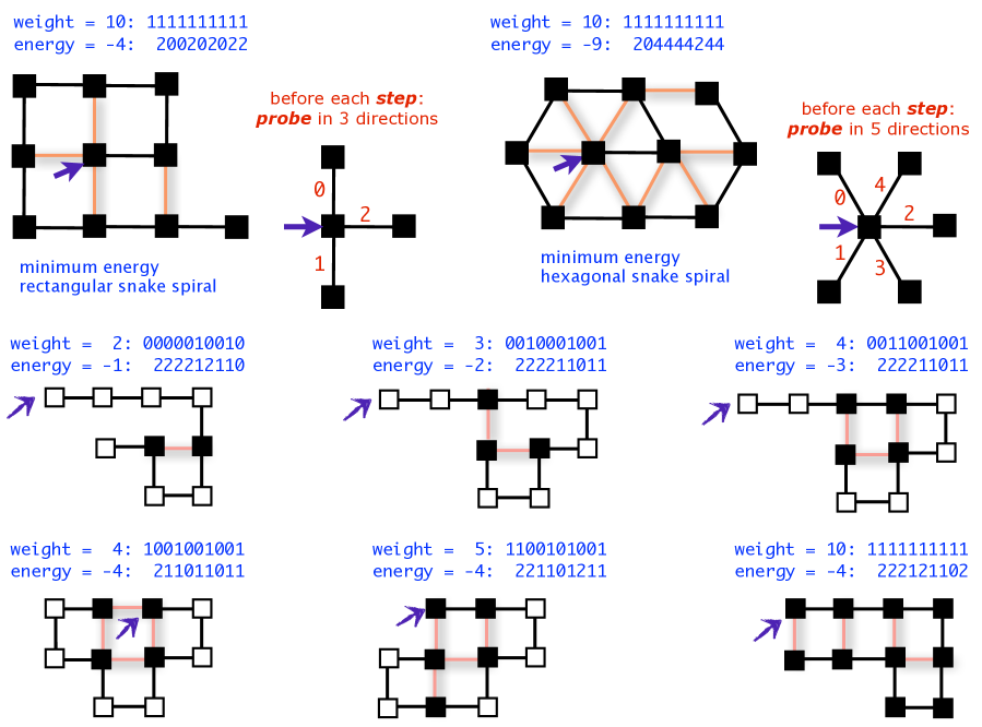
Let us take $n$ beads in $k$ colors, arrange them into a linear chain of length $n$ and register the position and the color of each bead, then allow the chain to fold onto a predefined grid in a space of 2 or 3 dimensions. The most popular model is the 2-color HP (hydrophobic and polar, black and white, ’1’ and ’0’) model, where any pair of H-type beads that are adjacent on the grid after folding forms a bond. We measure the quality of the folding by counting the number of such bonds in a given arrangement, called a conformation. Once we subtract this number from 0, we call the value energy of the folding and the objective of any folding optimization algorithm is to minimize the value of this energy. In Figure 4 we display a number of chains, each of length 10, where the number of black beads varies from 2 to 10 and the energy from -1 to -4 (the maximum possible). An additional characteristic of the chain is denoted as weight: it is simply the number of black beads in the chain.

On a 2-dimensional square lattice, each step of a SAW has a choice of at most 3 adjacent points of the grid: left, right, and forward, encoded as 0, 1, and 2. With the binary encoding of the colors and the ternary encoding of the self-avoiding walk to control the folding, we encode the coordinate for the folding problem for a chain of black and white beads of length $n$ as a concatenation of $n$ binary and $n-1$ ternary coordinates, defining a hyperhedron with a total of $(2^{n})\times(3^{n-1})$ face-centered vertices. As an alternative, we may also choose a more efficient hexagonal lattice which, when the chain is folded, will produce more bonds (the bees have done it!). In this case, there are 5 adjacent points on the grid; now the string of length $n$ is represented as a concatenation of $n$ binary and $n-1$ quinary coordinates, defining a hyperhedron with a total of $(2^{n})\times(5^{n-1})$ face-centered vertices.

Six folding experiments under the weight and energy target shown, with 1000 seeds each
binary	energy	beyond	unique	walkLength				probesPerStep
weight	target	target	solutions	median	mean	stdev	max	median	mean	stdev
2	-1	0	813	1000	843.6	695.5	2336	10.8	11.3	2.12
3	-2	0	511	39	338.0	580.7	2353	13	13.1	1.61
4	-3	95	204	26	104.1	290.7	2017	14.6	14.7	1.47
4	-4	0	2	797.5	1074.3	965.7	7433	13.9	14.0	0.82
5	-4	0	51	37.5	73.1	131.0	1755	15.8	16.0	1.27
10	-4	0	197	2	4.3	24.6	689	22	21.2	4.47

Figure 4: Empirical observations about the HP model of protein foldings in 2D with a chain of size 10 and SAWs: (1) lower bound on energy in rectangular grid is -4 (probes are made in 3 directions); (2) lower bound on energy in hexagonal grid is -9 (probes are made in 5 directions); (3) instances of 6 folding conformations in rectangular grid, each for a distinct pair of weight and energy target, define 6 classes of solutions; (4) walk length statistics and distributions, with a sample size of 1000 for each experiment. In order to find the postulated energy targets, an exhaustive enumeration or a Hamiltonian walk would visit, on the average, a total of $0.5*(2^{10}*3^{9}-1)=10,077,696$ coordinates under the rectangular grid formulation (compare with the maximum of 7433 in the table) and a total of $0.5*(2^{10*}5^{9}-1)=999,999,999$ coordinates under the hexagonal grid formulation. Our hypothesis: compared to the results shown here, the hexagonal grid may exhibit an energy landscape where SAWs will find energy minima in less steps on the average.

Table 1: Statistical experiments with SAWs to solve, under Plan A, Plan B and Plan C, the HP model of protein folding in 2D on a square lattice. The input parameters for each plan are: Chain size = 10; Energy target = -4; either fixed binary coordinate coordB of weight 4 (plan A); or fixed ternary coordinate coordT (plan B); or both initialized randomly (plan C). Experiments are performed with 1000 initial coordinates for each plan, and both the energy target of -4 and the binary weight target of 4 are reached under each plan, always returning only one binary solutions and two ternary solutions. Walk lengths under each plan differ significantly, with plan C representing the hardest instance of the folding protein problem. This is also the problem where SAW is the most effective compared to the (hypothetical) hamiltonian walk.

Plan A		median	mean	stdev	min	max
Given coordB	cntProbe	244	330.6	302.4	10	1994
with weight = 4,	walkLength	25	33.7	31.4	1	205
FIND coordT	probesPerStep	10	10.4	1.2	7.9	16
coordB = 1001001001
coordT =  200100100	The average walkLength to reach one of the two coordT
coordT =  211011011	under Hamiltonian walk = $0.25(3^{9}-1)=4921$

Plan B		median	mean	stdev	min	max
Given coordT,	cntProbe	26	34.0	15.6	1	127
FIND coordB	walkLength	4	5.2	2.4	0	20
with weight = 4	probesPerStep	6.5	6.5	0.49	1	8.5
coordT =  211011011	The average walkLength to reach the single coordB
coordB = 1001001001	under Hamiltonian walk = $0.5(2^{10}-1)=511$

Plan C		median	mean	stdev	min	max
FIND coordB,	cntProbe	10564.5	14187.8	12787.2	35	81156
with weight = 4	walkLength	752.5	1027.1	936.3	2	5936
& FIND coordT	probesPerStep	13.9	14.0	0.7	12.0	19.6
coordB = 1001001001
coordT =  200100100	The average walkLength to reach one of the two coordT
coordT =  211011011	under Hamiltonian walk = $0.25*(2^{10}*3^{9}-1)=5038848$

In this paper, we experiment with foldings on a 2-dimensional square lattice. We have grouped our experiments under three plans:

Plan A

Strech a chain of length $n$ with weight $w$ and assign the $w$ black beads into fixed positions. Represent this chain as a binary coordinate of length $n$ and weight $w$. Search for folding of this chain on a square lattice in 2D that will minimize its energy. Represent the solution as a ternary coordinate of length $n-1$.

Plan B

Fold a chain of length $n$ with weight $w=n$ into a preferred conformation. Typically, the preferred conformation is the one where the energy, with all beads being black, is the global minimum. Two such conformations, with all beads being black and the energy of -4, are shown in Figure 4. Now, represent this conformation as ternary coordinate of length $n$. Search for a binary coordinate of weight $w<n$ that either retains the minimum energy under all beads being black or is as close as possible to this value.

Plan C

Select the length of the chain $n$, its weight $w<=n$, and the target energy value that can be satisfied with at least one feasible folding conformation. Assign a random binary string of length $n$ and weight $w$ as the initial binary coordinate. Assign a random ternary ternary string of length $n-1$ as the initial ternary coordinate. Chances are that some initial ternary coordinates do not represent a feasible folding – this is not an issue since in our formulation, the search escapes the unfeasible regions effectively. The search now proceeds by probing simultaneously segments of each concatenated coordinate: the binary segment and the ternary segment before returning a feasible solution with the given weight and the energy target value.

Plan A represents the traditional formulation of the folding problem and many experimental results are reported under this plan. Plan B is also known as the inverse folding problem formulation and experimental results are also reported under this plan. A number of experiments that rely on exhaustive enumeration have similarities with Plan C. However, we are not aware of any publication of experimental results as described under Plan C in this paper; if brought to our attention, we shall report on them in our future publication.

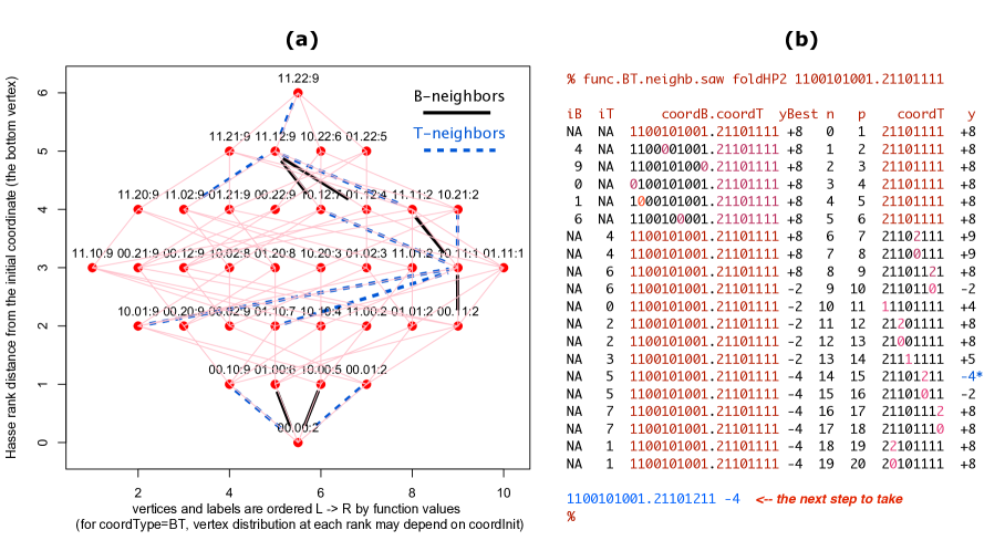
Introduced in Figure 1, labels in this graph are a a concatenation of binary coordinates and ternary coordinates. Each binary coordinate always has a neighborhood of 2 (dotted edges) while the neighborhood of ternary coordinate can vary from 2 to 4 (solid edges). For example, the coordinate 00.00 has 2 binary and two ternary neighbors; the coordinate 10.11 has 2 binary and 4 ternary neighbors.

Indices $iB$ and $iT$ that address values in binary and ternary coordinates are always randomly permuted in order to prevent biasing the order of choices for best function value yBest. Function values $y>0$ represent not only unfeasible conformations but also the relative level of unfeasibility. The counters $n$ and $p$ report the size of the neighborhood and the number probes to find each value of $y$.

Figure 5: An example of neighborhood calculation from an initial pivot coordinate (1100101001.21101111) that leads, in a single step, to an optimal conformation depicted in Figure 4.

The summary of statistical experiments in Figure 4 reveals a number of interesting properties. All have been performed under Plan C, with 1000 randomly selected initial configurations for each of the six weight and energy input pairs:

• As the tabulated binary weight increases and the energy target value decreases, the number of unique solution decrease from 813 (out of 1000 trials) to 2 (for weight = 4 and energy = -4), but then increase to 197 (for weight = 10 and energy = 4). The walkLength statistics varies significantly for each case – as does the distribution, which is bimodal, heavy-tailed, and clearly geometric for the case of only 2 unique solutions with weight = 4 and energy = -4.

• The beneficial side-effect our testing strategy is revealed for the case of weight = 4 and energy target = -3. Out of 1000 trials, there are 95 conformations with energy = -4, i.e. the returned solution is better than the target solution of -3. These solutions are in the class of ’rare solutions’ where only two unique solutions have been reported after 1000 trials for weight = 4 and energy = -4. We shall take advantage of this strategy also when performing experiments on longer chains which are summarized in Section IV.

We complete this subsection with the summary of results under Plan A, Plan B, and Plan C, shown in Table 1. Notably, the search with SAW under the plan B (the inverse folding formulation) is significantly easier than the search under Plan A (the traditional folding formulation). However, the search with SAW under Plan C requires significantly more steps than the Plan A and Plan B combined. The experiment under Plan C in Table 1 is a replication, under a different initial seed, of the experiment in Figure 4 in the row weight = 4, energy = -4.

Global stochastic search under SAW. We now briefly formalize coordinate neighborhoods, walks, and self-avoiding walks, concluding with a concise pseudo code that is the basis for our prototype solver on stochastic search under SAW.

Coordinate neighborhood. Formally, a neighborhood of a coordinate ${\underline{\varsigma}}_{j}$ is a set of coordinates

$${\cal N}({\underline{\varsigma}}_{j})=\{~{}{\underline{\varsigma}}_{j}^{i}~{}|~{}d({\underline{\varsigma}}_{j},{\underline{\varsigma}}_{j}^{i})=1,~{}~{}~{}i=1,2,\dots,L_{j}~{}\}$$ (1)

where $d({\underline{\varsigma}}_{j},{\underline{\varsigma}}_{j}^{i})$ is the rank distance between coordinates. The coordinate ${\underline{\varsigma}}_{j}$ is also called a pivot coordinate, has $L_{j}$ neighbors, each a distance of 1 from the pivot coordinate. In Figure 5-a we illustrate a Hasse graph that highlights three neighborhoods. Coordinates in this graph are a concatenation of binary coordinates of length 2 and ternary coordinates of length 2. Each binary coordinate always has a neighborhood of 2 (dotted edges) while the neighborhood of ternary coordinate can vary from 2 to 4 (solid edges). For example, the coordinate 00.00 has 2 binary and two ternary neighbors; the coordinate 10.11 has 2 binary and 4 ternary neighbors.

In Figure 5-b we illustrate the dynamics of neighborhood evaluations for an instance shown in Figure 4. We could not possibly have drawn a Hasse graph for this instance, however the principle of binary and ternary neighborhoods illustrated in Figure 5-a are the same.

What we can show is the trace of the entire neighborhood evaluation that takes place: starting with the pivot coordinate 1100101001.21101111, the best coordinate of the next pivot in this neighborhood is 1100101001.21101211 since it has the best energy conformation of -4. The trace also shows values of the objective function for various conformations – all values that are > 0 represent conformations that would lead to a conflict during folding; penalties values are assigned at different levels: +8 (initial pivot), +9, +8, +4, etc. Not all binary coordinates have been evaluated due to an input requirement that weight <= 5. The situation where a pivot would get trapped by adjacent pivots and the neighborhood would become empty did not yet arise.

1:$s\leftarrow 1901$ $\triangleright$ initial seed 2:${\underline{\xi}}_{0}\leftarrow coordInit(s)$ $\triangleright$ initial coordinate 3:$\Theta({\underline{\xi}}_{0})\leftarrow{\underline{\xi}}_{0}$ $\triangleright$ initial value 4:${\underline{\xi}^{*}}\leftarrow{\underline{\xi}}_{0}$ $\triangleright$ initial best coordinate 5:$\Theta({\underline{\xi}^{*}})\leftarrow{\underline{\xi}^{*}}$ $\triangleright$ initial best value 6:$\omega\leftarrow 0$ $\triangleright$ initial walk length 7:$\Theta^{ub}_{L}\leftarrow 0$ $\triangleright$ initial upper bound 8:$\tau\leftarrow 1$ $\triangleright$ initial cntProbe 9:$\tau_{lmt}\leftarrow 2^{24}$ $\triangleright$ cntProbe limit value 10:$isCens\leftarrow 0$ $\triangleright$ initialize as uncensored 11:if $\Theta({\underline{\xi}^{*}})\leq\Theta^{ub}_{L}$ then 12:     $Table\leftarrow(s,{\underline{\xi}^{*}},\Theta({\underline{\xi}^{*}}),\tau,\omega,isCens)$ ; return 13:end if 14:while $\Theta({\underline{\xi}^{*}})>\Theta^{ub}_{L}$ do 15:     if $\tau==\tau_{lmt}$ then 16:         $isCens\leftarrow 1$ ; break 17:     else 18:         $\omega=\omega+1$ $\triangleright$ a new step! 19:         $temp\leftarrow{\tt coordUpdate}({\underline{\xi}}_{\omega-1},\tau)$ 20:         ${\underline{\xi}}_{\omega}:\Theta({\underline{\xi}}_{\omega}):\tau\leftarrow temp$ 21:         if $\Theta({\underline{\xi}}_{\omega})\leq\Theta({\underline{\xi}^{*}})$ then 22:              ${\underline{\xi}^{*}}\leftarrow{\underline{\xi}_{\omega}}$ 23:              $\Theta({\underline{\xi}^{*}})\leftarrow{\underline{\xi}^{*}}$ 24:         end if 25:     end if 26:end while 27:if $isCens==1$ then 28:     $Table\leftarrow(s,{\underline{\xi}^{*}},\Theta({\underline{\xi}^{*}}),\tau,\omega,isCens)$ 29:else 30:     if $\Theta({\underline{\xi}^{*}})==\Theta^{ub}_{L}$ then 31:         $Table\leftarrow(s,{\underline{\xi}^{*}},\Theta({\underline{\xi}^{*}}),\tau,\omega,isCens)$ 32:     else 33:         $\Theta^{ub}_{L}\leftarrow\Theta({\underline{\xi}^{*}})$ $\triangleright$ Better upper bound! 34:         $Table\leftarrow(s,{\underline{\xi}^{*}},\Theta({\underline{\xi}^{*}}),\tau,\omega,isCens)$ 35:     end if 36:end if

The procedure coordUpdate.saw takes the pivot coordinate, the probe counter and the walk list. In Step 6, it computes, in random order, the neighborhood ${\cal N}({\underline{\varsigma}}_{\omega-1})$ of all adjacent coordinates. The order randomization ensures that all coordinates get an equal chance of selection; without it, some paths in the Hasse graph may never be taken, thereby inducing a bias in the average walk length. The Step 7 eliminates all adjacent coordinates that may have been used as pivots already and returns a neighborhood subset ${\cal N}_{r}({\underline{\varsigma}}_{\omega-1})$. If the neighborhood subset is not empty, the procedure bestNeighbor in Step 9 probes all coordinates in the subset and returns the new pivot as the coordinate:value pair with the ‘best value’, along with the incremented value of $\tau$, updates the walk list to $Walk_{\omega}$ in Step 10, and exits on Step 18. An empty neighborhood implies that the SAW is trapped, i.e. the selection of the pivot for the next step is blocked by adjacent coordinates that are already pivots. Subsequently, a new walk segment is initialized with a random coordinate in Step 15. The procedure exits with the expected parameter values on Step 16. 1:$\omega\leftarrow\omega+1$ 2:$Walk_{\omega-1}\leftarrow\{{\underline{\varsigma}}_{0},~{}{\underline{\varsigma}}_{1},~{}{\underline{\varsigma}}_{2},~{}\dots,~{}{\underline{\varsigma}}_{\omega-1}\}$ 3:procedure coordUpdate.saw(${\underline{\varsigma}}_{\omega-1},\tau,Walk_{\omega-1})$ 4:     $\mathbb{Z}\leftarrow i=1,2,\ldots,L$ 5:     $\mathbb{Z}_{p}\leftarrow permute(\mathbb{Z})$ 6:     ${\cal N}({\underline{\varsigma}}_{\omega-1})\leftarrow\{{\underline{\varsigma}}_{\omega-1}^{i}~{}|~{}d({\underline{\varsigma}}_{\omega-1},{\underline{\varsigma}}_{\omega-1}^{i})=1,~{}i\in\mathbb{Z}_{p}\}$ 7:     ${\cal N}_{r}({\underline{\varsigma}}_{\omega-1})\leftarrow\{{\cal N}({\underline{\varsigma}}_{\omega-1})~{}|~{}{\underline{\varsigma}}_{\omega-1}^{i}\not\in Walk_{\omega-1}\}$ 8:     if ${\cal N}_{r}\not=\emptyset$ then 9:         $\!\!\!\!{\underline{\varsigma}}_{\omega}\!\!:\!\Theta({\underline{\varsigma}}_{\omega})\!:\!\tau\leftarrow bestNeighbor({\cal N}_{r},{\underline{\varsigma}}_{\omega-1},\tau_{\omega-1})$ 10:         $\!\!\!\!Walk_{\omega}\leftarrow\{{\underline{\varsigma}}_{0},~{}{\underline{\varsigma}}_{1},~{}{\underline{\varsigma}}_{2},~{}\dots,~{}{\underline{\varsigma}}_{\omega-1},~{}{\underline{\varsigma}}_{\omega}\}$ 11:     else$\triangleright$ trapped pivot, restart 12:         $\!\!\!\!s\leftarrow randomSeed()$ 13:         $\!\!\!\!{\underline{\varsigma}}_{0}\leftarrow coordInit(s)$ $\triangleright$ new initial coord. 14:         $\!\!\!\!\Theta({\underline{\varsigma}}_{0})\leftarrow{\underline{\varsigma}}_{0}$ $\triangleright$ new initial value 15:         $\!\!\!\!Walk_{0}\leftarrow\{{\underline{\varsigma}}_{0}\}$ $\triangleright$ new walk segm. 16:         ​​​​return ${\underline{\varsigma}}_{0}\!\!:\!\Theta({\underline{\varsigma}}_{0})\!:\!\tau\!:\!Walk_{0}$ 17:     end if 18:     return ${\underline{\varsigma}}_{\omega}\!\!:\!\Theta({\underline{\varsigma}}_{\omega})\!:\!\tau\!:\!Walk_{\omega}$ 19:end procedure

Figure 6: The walk as a part of the global stochastic search process: the walk stops (1) upon reaching the best upper bound, returning a new or already known solution coordinate, or (2) upon finding a new best upper bound, returning a new best solution coordinate, or (3) upon exceeding the allocated time of counter limit, returning a new or already known censored solution coordinate and a value above the upper bound. The procedure that controls the performance of the walk, here a self-avoiding walk, is named coordUpdate.

Contiguous walks and SAWs. Let the coordinate ${\underline{\varsigma}}_{0}$ be the initial coordinate from which the walk takes the first step. Then the sequence

$$\{{\underline{\varsigma}}_{0},{\underline{\varsigma}}_{1},{\underline{\varsigma}}_{2},\dots,{\underline{\varsigma}}_{j},\dots,{\underline{\varsigma}}_{\omega}\}$$ (2)

is called a walk list or a walk of length $\omega$, the coordinates ${\underline{\varsigma}}_{j}$ are denoted as pivot coordinates and $\Theta({\underline{\varsigma}}_{j})$ are denoted as pivot values. Given an instance of size $L$ and its best upper bound $\Theta^{ub}_{L}$, we say that the walk reaches its target value (and stops) when $\Theta({\underline{\varsigma}}_{\omega})=\Theta^{ub}_{L}$.

We say that the walk is contiguous if the rank distance between adjacent pivots is 1; i.e. we find

$$d({\underline{\varsigma}}_{j},{\underline{\varsigma}}_{j-1})=1,~{}~{}~{}j=1,2,...,\omega$$

We say that the walk is self-avoiding if all pivots in (2) are unique. We say that the walk is composed of two or more walk segments if the initial pivot of each walk segment has been induced by a well-defined heuristic such as random restarts. Walk segments can be of different lengths and if viewed independently of other walks, may be self-avoiding or not. A walk composed of two or more self-avoiding walk segments may no longer be a self-avoiding walk, since some of the pivots may overlap and also form cycles.

Global stochastic search under SAW. The pseudo-code in Figure 6 formalizes the global search algorithm that relies on SAW as its search engine. The code forms the basis for the prototype solver not only for the porting folding instances experiments in this paper but also for a number of other problem instance as outlined in Section I.

IV.   Summary of Experiments

Experimental results, summarized in Figure 7, Figure 8, and Table 2, can only be descried briefly.

The motivation for the experiment in Figure 7 came from [18]:

Instance: An integer $n$ and a finite sequence of $S$ over the alphabet $\{H,P\}$ which contains $n^{3}$ $H$’s.
Question: Is there a fold of $S$ in $\mathbb{Z}^{3}$ for which H’s are perfectly packed into an $n\times n\times n$ cube?

This problem has been proven to be NP-hard and the more general problem as NP-complete.

The spiral chain in Figure 7 can be considered as a simpler case of the perfect HP problem posited for a 3-D cube in [18]. In our context, we ask: how many conformations can be found with the same energy and how hard is it to find them? The answers that we display in Figure 7 are somewhat surprising and will be analyzed in more depth later.

Figure 7: The spiral chain can be considered as a simpler case of the perfect HP problem posited for a 3-D cube in [18]. In our context, we ask: how many conformations can be found with the same energy and how hard is it to find them? Some of the answers can be gleaned from the asymptotic performance of the SAW solver in terms of the required walkLength to reach the minimum energy targets of (-9, -10, …, -16) for chain lengths for L = (15, 17, …, 25). It appears that there are clear different walkLength performance regimes when solving with L = (16, 20, 25) when compared to solving with other values of L.

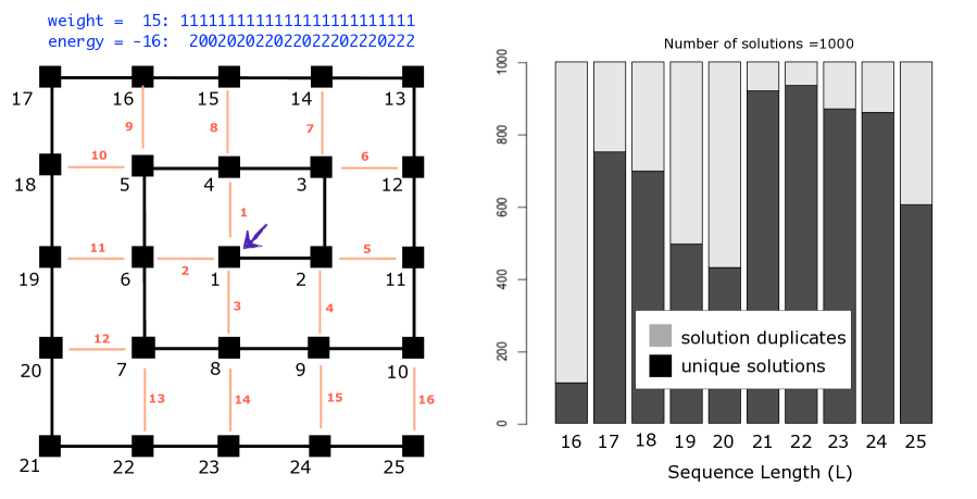
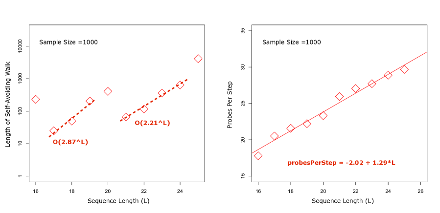
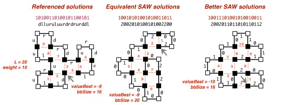
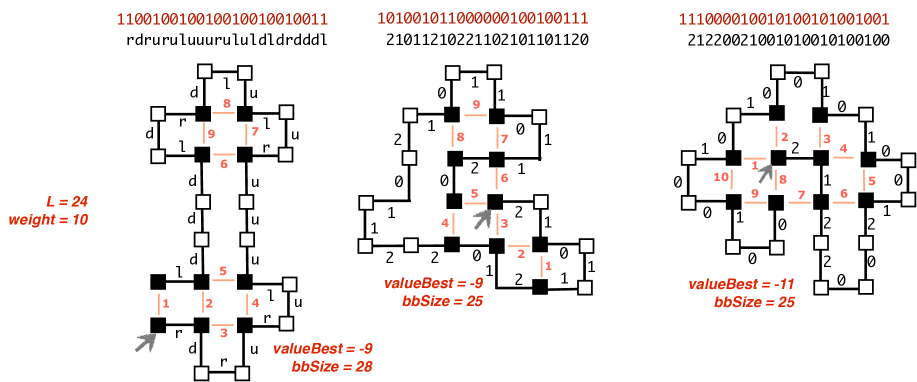
Experiments performed on well-known instance classes under Plan A and Plan C are summarized in Figure 8 and Table 2. The main objectives are:

1. Under Plan A: replicate experiments to achieve the same or better target energy values published for standard instances with chains of length of 20, 24, and 25, given a fixed binary coordinate [19], [20]. Return solutions as ternary coordinates.

2. Under the first Plan C: find simultaneously, the pair of binary and ternary coordinates that maintain the weight of binary coordinates under Plan A – at the same or better target energy values.

3. Under the second Plan C: find simultaneously, the pair of binary and ternary coordinates that maintain the weight of binary coordinates under Plan A and exceed the energy target value found under the first experiments of Plan C.

Figure 8: Comparisons of protein folding conformations for chain lengths of 20, 24, and 25. instance conformation in the column ‘Referenced solutions’ are from from [19] and [20] and have been reported under what we call Plan A in this paper. Instances under the column ‘Equivalent SAW solutions’ are alternative foldings obtained by our SAW solver under Plan C and the same energy targets as shown for ‘Referenced solutions’. Instances under the column ‘Better SAW solutions’ are alternative foldings obtained by our SAW solver under Plan C and better energy targets: -10 vs -9 for L=20; -11 vs -9 for L=24, and -10 vs -8 for L=25.

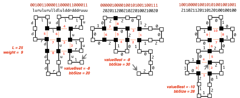
Our findings so far:

• Under Plan A, our experiments replicate but not improve published energy target values.

• Under the first Plan C, our experiments generate up to 990 (out of 1000 initiated) new and unique solutions. In most cases, energy values remain the same as for Plan A. However, there also are improvements that lead to experiments under the second Plan C.

• Under the second Plan C, experiments with improved energy targets generate from 11 to 875 unique solutions with the assigned energy target value, except for the chain of length 24, where again, an improved energy target value is observed for two instances.

Table 2: Statistical summary of experiments, a companion to Figure 8. Experiments under ‘Referenced solutions’ are under Plan A as defined in the paper. Experiments under ‘Equivalent SAW solutions’ and ‘Better SAW solutions’ are under Plan C. All experiments, except for the one flagged in the footnote, are based on a sample size of 1000. As an additional bonus, we also found another improved solution while running the case of L = 24, weight = 10, energy = 10. The energy improved from -10 to -11 and it is this conformation which shown in Figure 8.

	Reference solutions				Equivalent SAW solutions				Better SAW solutions
	energy	walkLength			energy	walkLength			energy	walkLength
instance	target	median	mean	stdev	target	median	mean	stdev	target	median	mean	stdev
length = 20
weight = 10	-9	2079	3097	2890.8	-9	315	812	1183.0	-10	9742	15088	16364
unique sols	4				928				109
length = 24
weight = 10	-9	957	1575	1765	-9	649	4104	54529	-10	9059	19391	26142
unique sols	35				975				875
length = 25
weight = 9	-8	13099	21557	27639	-8	959.5	9679	95154	-10	933928	1243210	1087628
unique sols	32				990				11$\dagger$

($\dagger$) Statistics for the pair (weight = 9, energy target = -10) are based on the sample size of 62
(rather than 1000) as is the case with other entries in this table.

V.   Conclusions And Future Work

Our experiments with the SAW solver raise the expectation that the solution of the protein folding problem, where the chain configuration and its confirmation are optimized simultaneously, may be feasible at an acceptable cost. One of the best way to accelerate improvements is cooperate with other researchers so that solver implementations can be compared side-by-side for their strengths and weaknesses, following the example in [9].

Experiments are being planned also for triangular and hexagonal grids in 2- and 3-dimensions.

References

- [1] N. Metropolis, A. W. Rosenbluth, M. N. Rosenbluth, A. H. Teller, and E. Teller. Equation of State Calculations by Fast Computing Machines. Journal of Chemical Physics, 21:1087–1092, June 1953.
- [2] W. K. Hastings. Monte Carlo sampling methods using Markov chains and their applications. Biometrika, 57(1):97–109, 1970.
- [3] M. P. Vecchi S. Kirkpatrick, D. Gelatt Jr. Optimization by simulated annealing. Science, 220(5-6):671–680, 1983.
- [4] Wikipedia. Simulated Annealing, Nov 2013.
- [5] Stuart Geman and Donald Geman. Stochastic relaxation, Gibbs distributions and the Bayesian restoration of images. IEEE Transactions on Pattern Analysis and Machine Intelligence, 6(6):721–741, November 1984.
- [6] Fred Glover. Tabu Search – Part I. ORSA Journal on Computing, 1(3):190–206, 1989.
- [7] Fred Glover. Tabu Search – Part II. ORSA Journal on Computing, 2(1):4–32, 1990.
- [8] Franc Brglez. Of n-dimensional Dice, Combinatorial Optimization, and Reproducible Research: An Introduction. Eletrotehniški Vestnik 78(4): 181–192, English Edition,, 78(4):181–192, 2011, http://ev.fe.uni-lj.si/4-2011/Brglez.pdf.
- [9] Borko Bošković, Franc Brglez, and Janez Brest. Low-Autocorrelation Binary Sequences: on the Performance of Memetic and Self-Avoiding Walk Solvers. arxiv.org, Journal Submission, 2013, (A preprint available on request).
- [10] Sorin Istrail and Fumei Lam. Combinatorial Algorithms for Protein Folding in Lattice Models: A Survey of Mathematical Results. Commun. Inf. Syst.,, 9:303–346, 2009.
- [11] D. I. McCooey. Java Applets for Visualizing Polyhedra. http://www.dmccooey.com/polyhedra/, September 2013.
- [12] Wikipedia. Self-avoiding walk, July 2013.
- [13] S. Hemmer and P.C. Hemmer. An average self-avoiding random walk on the square lattice lasts 71 steps. J. Chem. Phys., 81(1):584–586, 1984.
- [14] Gordon Slade. Self-Avoiding Walks. The Mathematical Intelligencer, 16(1), 1994.
- [15] Linus Pauling. General Chemistry. Dover Publications, 1970.
- [16] Nathan Clisby. Efficient Implementation of the Pivot Algorithm for Self-avoiding Walks. Journal of Statistical Physics, 140:349–392, July 2010.
- [17] Brian Hayes. Prototeins. AmSci, 86(3):216–221, 1998.
- [18] Bonnie Berger and Tom Leighton. Protein folding in the hydrophobic-hydrophilic (HP) model is NP-complete. J. Comp Bio, 5:27—40, 1998.
- [19] Ron Unger and John Moult. Genetic Algorithms for Protein Folding Simulations. Journal of Molecular Biology, 231(1):75 – 81, 1993.
- [20] Thang N. Bui and Gnanasekaran Sundarraj. An efficient genetic algorithm for predicting protein tertiary structures in the 2D HP model. In GECCO ’05, pages 385–392. ACM, 2005.