When to Sell a Markov Chain Asset?

Abstract

This paper is concerned with an optimal stock selling rule under a Markov chain model. The objective is to find an optimal stopping time to sell the stock so as to maximize an expected return. Solutions to the associated variational inequalities are obtained. Closed-form solutions are given in terms of a set of threshold levels. Verification theorems are provided to justify their optimality. Finally, numerical examples are reported to illustrate the results.

Key words: Markov chain asset, optimal stopping, quasi-variational inequalities

1 Introduction

Most market models in the literature are Brownian motion based including geometric Brownian motion, diffusion with possible jumps and regime switching; see related books by Duffie [2], Hull [7], Elliott and Kopp [3], Fouque et al. [4], Karatzas and Shreve [8], and Musiela and Rutkowski [11] among others. An alternative is the binomial tree model introduced by Cox-Ross-Rubinstein. The BTM is natural for financial markets because intensive buying moves the market upwards and forceful selling pushes it downwards. All these transactions take place in discrete moments. However, a main drawback of the BTM is its non-Markovian nature, which makes it difficult to work with mathematically. In this paper, we consider a Markov chain market model. The main advantage of such a model is it preserves much of the flexibility of the binomial tree structure and, in the meantime, it is more mathematically tractable, which allows serious mathematical analysis in related optimization problems. Recently, several Markov chain based models are developed. For example, van der Hoek and Elliott [14] introduced a stock price model based on stock dividend rates and a Markov chain noise. Norberg [12] used a Markov chain to represent interest rate and considered a market model driven by a Markov chain. In particular, the market model in [12] resembles a GBM in which the ‘drift’ is approximated by the duration between jumps and the ‘diffusion’ is given in terms of jump times. An additional advantage of a Markov chain driven model is its price is almost everywhere differentiable. Such differentiability is desirable in an optimal control type analysis proposed by Barmish and Primbs [1]. In connection with dynamic programming problems, the corresponding Hamilton-Jacobi-Bellman equations are of first order, which are easier to analyze than those under traditional Brownian motion based models. Finally, the Markov chain model is not that far apart from a GBM because it can be used to approximate a GBM by varying its jump rates. In fact, it is shown in Example 1 that a properly scaled Markov chain model converges weakly to that of a GBM as the jump rates go to infinity.

When to sell a stock is a crucial component in stock trading. It determines when to take profits or to cut losses. It is probably the most emotional part for individual investors in the trading process. Selling rules in financial markets have been studied for many years. For example, Zhang [18] considered a selling rule determined by two threshold levels: a target price and a stop-loss limit. One makes a selling decision whenever the price reaches either levels. Under a switching GBM, the objective is to determine these threshold levels to maximize an expected discounted reward function. In [18], such optimal threshold levels are obtained by solving a set of two-point boundary value problems. In Guo and Zhang [5], they considered the optimal selling rule under a GBM model with regime switching. Using a smooth-fit technique, they were able to convert the optimal stopping problem to a set of algebraic equations. These algebraic equations were used to determine the optimal target levels. In addition to these analytical results, various mathematical tools have been developed to compute these threshold levels. For example, a stochastic approximation technique was used in Yin, Liu and Zhang [15] and a linear programming approach was developed in Helmes [6]. In addition, Merhi and Zervos [10] studied an investment capacity expansion/reduction problem following a dynamic programming approach under a GBM market model. Similar problem under a more general market model was treated by Løkka and Zervos [9].

In this paper, the stock price is assumed to follow a Markov chain model. Under this model, the state of the Markov chain can be estimated based on the stock price increments. This makes the Markov chain observable. In addition to its simplicity, the Markov chain model is able to capture price movements of a broader range of stocks. In this paper, under the Markov chain model, we consider an optimal stock selling rule and obtain its solution in terms of a set of threshold levels. In particular, we solve the corresponding dynamic programming problem and obtain these threshold levels. We point out that the standard smooth-fit method that works in a GBM setting is not adequate in one of the cases in this paper because of the lack of enough equations for the unknown parameters. To solve the problem, we need to explore other convexity conditions to determine uniquely these parameters. We also provide a set of sufficient conditions that guarantee their optimality. Numerical examples are reported to illustrate these results.

This paper is organized as follows. In §2, we formulate the problem and make a few assumptions. In §3, we study properties of the value functions, the associate HJB equations, and their solutions. In §4, we provide a set of sufficient conditions that guarantee the optimality of our selling rule. We also include three numerical examples in this section. Some concluding remarks are given in §5. Some technical results are provided in an appendix.

2 Problem Formulation

Let $\{\alpha_{t}:\ t\geq 0\}$ denote a two-state Markov chain with state space ${\cal M}=\{1,2\}$ and generator $Q=\left(\begin{array}[]{cc}-\lambda_{1}&\lambda_{1}\\[-7.22743pt] \lambda_{2}&-\lambda_{2}\\ \end{array}\right)$, for given $\lambda_{1}>0$ and $\lambda_{2}>0$. Let $S_{t}$ denote the stock price at time $t$ given by the equation

$$\frac{dS_{t}}{S_{t}}=f(\alpha_{t})dt,\ S_{0}=x\geq 0,\ t\geq 0,$$

where $f(1)=f_{1}>0$ represents the uptick return rate and $f(2)=f_{2}<0$ the downtick return rate. Let ${\cal F}_{t}=\{S_{r}:\ r\leq t\}$ denote the filtration generated by $S_{t}$. Note that $\alpha_{t}$ is observable and ${\cal F}_{t}=\{\alpha_{r}:\ r\leq t\}$.

Let $K$ denote the fixed transaction cost. Given $S_{0}=x$ and $\alpha_{0}=i\in{\cal M}$, the objective of the problem is to choose an ${\cal F}_{t}$ stopping time $\tau$ so as to maximize

$$J(x,i,\tau)=E\left(e^{-\rho\tau}(S_{\tau}-K)I_{\{\tau<\infty\}}\right),$$

where $\rho>0$ is the discount factor.

Let $V(x,i)=\sup_{\tau}J(x,i,\tau)$ be the value function. Then it is easy to see that $V(x,i)\geq 0$, $V(0,i)=0$, $i=1,2$. Moreover, $V(x,i)$ is convex in $x$ for fixed $i=1,2$.

Let $\Phi(\rho)=(\rho+\lambda_{1}-f_{1})(\rho+\lambda_{2}-f_{2})-\lambda_{1}\lambda_{2}$. Then the bigger root of $\Phi(\rho)=0$ is given by

$$B_{0}=\frac{1}{2}\left(f_{1}-\lambda_{1}+f_{2}-\lambda_{2}+\sqrt{((f_{1}-\lambda_{1})-(f_{2}-\lambda_{2}))^{2}+4\lambda_{1}\lambda_{2}}\right).$$

Note that if $\rho\leq B_{0}$, then following similar argument as in Guo and Zhang [5], we can show that it is optimal not to sell at all. In the rest of this paper, we only consider the case when $\rho>B_{0}$, which implies $\Phi(\rho)>0$. We summarize the conditions to be imposed in the rest of this paper:

• (A1) $f_{1}>0$ and $f_{2}<0$;

• (A2) $\Phi(\rho)>0$.

Let $\displaystyle(\nu_{1},\nu_{2})=\left({\lambda_{2}}/{(\lambda_{1}+\lambda_{2})},{\lambda_{1}}/{(\lambda_{1}+\lambda_{2})}\right)$ denote the stationary distribution of $\alpha_{t}$ and let $\mu=\nu_{1}f_{1}+\nu_{2}f_{2}$. Then, $f_{2}<\mu<f_{1}$. Moreover, it is easy to see that $\Phi(\mu)=(\mu-f_{1})(\mu-f_{2})<0$. This implies $B_{0}>\mu$. Therefore, $\rho>\mu$.

Note that, for any ${\cal F}_{t}$ stopping time $\tau$,

$$J(x,i,\tau)=xE\left(e^{-\rho\tau}\exp\int_{0}^{\tau}f(\alpha_{s})ds\right)I_{\{\tau<\infty\}}-KEe^{-\rho\tau}.$$

In order to have finite $V(x,i)$, necessarily

$$\sup_{\tau}E\left(e^{-\rho\tau}\exp\int_{0}^{\tau}f(\alpha_{s})ds\right)I_{\{\tau<\infty\}}<\infty.$$

In view of this, $V(x,i)$ needs to be at most linear growth in $x$. In addition, note that the stock price $S_{t}$ is differentiable and the value of $\alpha_{t}$ can be given in terms of the derivative of $\log(S_{t})$.

3 HJB Equations

Let ${\cal A}$ denote the generator of $(S_{t},\alpha_{t})$, i.e., for any differentiable functions $h(x,i)$, $i=1,2$,

$$\left\{\begin{array}[]{l}\displaystyle{\cal A}h(x,1)=xf_{1}h^{\prime}(x,1)+\lambda_{1}(h(x,2)-h(x,1)),\\[7.22743pt] \displaystyle{\cal A}h(x,2)=xf_{2}h^{\prime}(x,2)+\lambda_{2}(h(x,1)-h(x,2)),\\ \end{array}\right.$$

where $h^{\prime}$ denotes the derivative of $h$ with respect to $x$. The associated HJB equations should have the form:

$$\left\{\begin{array}[]{l}\min\{\rho v(x,1)-{\cal A}v(x,1),\ v(x,1)-(x-K)\}=0,\\ \min\{\rho v(x,2)-{\cal A}v(x,2),\ v(x,2)-(x-K)\}=0.\end{array}\right.$$ (1)

In this section, we solve these HJB equations. First, if the price $S_{t}$ is small, then one should hold the position because the price is not attractive regardless $\alpha_{t}=1$ or 2. In view of this, we expect the existence of $x^{*}$ such that no selling is $S_{t}<x^{*}$. The corresponding interval $(0,x^{*})$ gives a continuation region. Note that $V(x,i)\geq 0$ implies $x^{*}\geq K$. On this interval, the equalities $\rho v(x,i)-{\cal A}v(x,i)=0$, $i=1,2$, must hold. Using the generator ${\cal A}$, we can write

$$\left\{\begin{array}[]{l}(\rho+\lambda_{1})v(x,1)=xf_{1}v^{\prime}(x,1)+\lambda_{1}v(x,2),\\ (\rho+\lambda_{2})v(x,2)=xf_{2}v^{\prime}(x,2)+\lambda_{2}v(x,1).\\ \end{array}\right.$$

Using the first equation, we write

$$v(x,2)=\frac{1}{\lambda_{1}}\left((\rho+\lambda_{1})v(x,1)-xf_{1}v^{\prime}(x,1)\right).$$

Substitute this into the second equation and simplify to obtain

$$x^{2}f_{1}f_{2}v^{\prime\prime}(x,1)+x(f_{1}f_{2}-D_{1})v^{\prime}(x,1)+D_{2}v(x,1)=0,$$ (2)

where

$$\left\{\begin{array}[]{l}D_{1}=(\rho+\lambda_{1})f_{2}+(\rho+\lambda_{2})f_{1},\\ D_{2}=(\rho+\lambda_{1})(\rho+\lambda_{2})-\lambda_{1}\lambda_{2}.\end{array}\right.$$ (3)

Let $\beta_{1}<0$ and $\beta_{2}>0$ denote the roots of

$$f_{1}f_{2}\beta^{2}-D_{1}\beta+D_{2}=0.$$ (4)

Then,

$$\left\{\begin{array}[]{l}\displaystyle\beta_{1}=\frac{D_{1}+\sqrt{D_{1}^{2}-4f_{1}f_{2}D_{2}}}{2f_{1}f_{2}}<0,\\[7.22743pt] \displaystyle\beta_{2}=\frac{D_{1}-\sqrt{D_{1}^{2}-4f_{1}f_{2}D_{2}}}{2f_{1}f_{2}}>0.\\ \end{array}\right.$$ (5)

The general solution to (2) can be given as

$$v(x,1)=A_{1}x^{\beta_{1}}+A_{2}x^{\beta_{2}},$$

for some constants $A_{1}$ and $A_{2}$.

On $(0,x^{*})$, the convexity condition implies that $v(x,1)$ is bounded. Necessarily, $A_{1}=0$. Therefore, $v(x,1)=A_{2}x^{\beta_{2}}$. Substitute this back into the first equation to obtain $v(x,2)=\kappa_{2}A_{2}x^{\beta_{2}}$, where $\kappa_{2}={(\rho+\lambda_{1}-f_{1}\beta_{2})}/{\lambda_{1}}$.

Recall that $\alpha_{t}$ is observable. One should hold the position longer under the condition $\alpha_{t}=1$ (uptick) than that under $\alpha_{t}=2$ (downtick). In view of this, we consider the HJB equations on $(x^{*},x_{0}^{*})$ for some $x_{0}^{*}>x^{*}$. The idea is to sell if $(S_{t},\alpha_{t})\in[x^{*},\infty)\times\{2\}$ and hold if $(S_{t},\alpha_{t})\in(0,x_{0}^{*})\times\{1\}$ till $S_{t}$ reaching $x_{0}^{*}$. Clearly, $v(x,2)=x-K$ and $\rho v(x,1)-{\cal A}v(x,1)=0$, on $(x^{*},x_{0}^{*})$. Using this, we solve the equation

$$\rho v(x,1)-{\cal A}v(x,1)=0,\\$$

which gives

$$(\rho+\lambda_{1})v(x,1)=xf_{1}v^{\prime}(x,1)+\lambda_{1}(x-K).$$

It is easy to see a particular solution

$$\phi_{0}(x)=A_{0}x+B_{0},\mbox{ where }A_{0}=\frac{\lambda_{1}}{\rho+\lambda_{1}-f_{1}}\mbox{ and }B_{0}=-\frac{\lambda_{1}K}{\rho+\lambda_{1}}.$$ (6)

Let $\gamma_{1}=(\rho+\lambda_{1})/f_{1}$. Then, the general solution can be given by

$$v(x,1)=C_{1}x^{\gamma 1}+\phi_{0}(x),$$

for any constant $C_{1}$.

Next we consider two separate cases to continue solving the HJB equations.

Case I: $\rho\leq f_{1}$

Assuming $\rho\leq f_{1}$, we first show that $x_{0}^{*}=\infty$. If not, we must have $v(x,1)=v(x,2)=x-K$ for $x>x_{0}^{*}$. In order to satisfy the HJB equations (1), $v(x,1)$ has to satisfy the inequality $\rho v(x,1)-{\cal A}v(x,1)\geq 0$, for $x>x_{0}^{*}$. Plugging $v(x,1)=v(x,2)=x-K$ in this inequality, we have

$$\rho(x-K)\geq xf_{1}.$$

Therefore, $(\rho-f_{1})x\geq\rho K$, for $x>x_{0}^{*}$. This contradicts $\rho\leq f_{1}$. Hence $x_{0}^{*}=\infty$.

In view of these, on $(x^{*},\infty)$, $v(x,1)=C_{1}x^{\gamma 1}+\phi_{0}(x)$ and $v(x,2)=x-K$. This means never sell when $\alpha_{t}=1$. Recall the linear growth property and nonnegativity of $v(x,i)$. It follows that $C_{1}=0$ because $\gamma_{1}>1$.

Next, we determine the values of $x^{*}$ and $A_{2}$. Recall that $v(x,1)$ and $v(x,2)$ are convex on $(0,\infty)$. Necessarily, they are continuous. In particular, they are continuous at $x=x^{*}$. Therefore,

$$\left\{\begin{array}[]{l}A_{2}(x^{*})^{\beta_{2}}=A_{0}x^{*}+B_{0},\\ \kappa_{2}A_{2}(x^{*})^{\beta_{2}}=x^{*}-K.\end{array}\right.$$

Solving these equations, we have

$$x^{*}=-\frac{K+\kappa_{2}B_{0}}{\kappa_{2}A_{0}-1},$$ (7)

and

$$A_{2}=\frac{A_{0}x^{*}+B_{0}}{(x^{*})^{\beta_{2}}}.$$ (8)

It is elementary to check that

$$x^{*}=\left(\frac{\rho+\lambda_{1}-f_{1}}{\rho+\lambda_{1}}\right)\left(\frac{K\beta_{2}}{\beta_{2}-1}\right).$$ (9)

The solutions to the HJB equations (1) should have the form:

$$\left\{\begin{array}[]{l}v(x,1)=\left\{\begin{array}[]{ll}A_{2}x^{\beta_{2}}&\mbox{ if }0\leq x\leq x^{*},\\ A_{0}x+B_{0}&\mbox{ if }x>x^{*},\\ \end{array}\right.\\ v(x,2)=\left\{\begin{array}[]{ll}\kappa_{2}A_{2}x^{\beta_{2}}&\mbox{ if }0\leq x\leq x^{*},\\ x-K&\mbox{ if }x>x^{*}.\\ \end{array}\right.\\ \end{array}\right.$$ (10)

Theorem 1

.  Assume $\rho\leq f_{1}$. Then the functions $v(x,i)$, $i=1,2$, given above are continuous on $(0,\infty)$ and differentiable on $(0,\infty)-\{x^{*}\}$. They satisfy the HJB equations (1). In particular, the following inequalities hold:

$$\left\{\begin{array}[]{ll}A_{2}x^{\beta_{2}}\geq x-K&\mbox{ on }(0,x^{*}),\\ \kappa_{2}A_{2}x^{\beta_{2}}\geq x-K&\mbox{ on }(0,x^{*}),\\ v(x,1)\geq x-K&\mbox{ on }(x^{*},\infty),\\ \rho v(x,2)-{\cal A}v(x,2)\geq 0&\mbox{ on }(x^{*},\infty).\end{array}\right.$$ (11)

Proof. It is sufficient to show these four inequalities. First, note that $\Phi(\rho)>0$ implies $\rho+\lambda_{1}-f_{1}>0$. Under the condition $\rho\leq f_{1}$, we have $A_{0}\geq 1$. The third inequality in (11) follows from $B_{0}>-K$. In addition, the first inequality follows from the second one because $0<\kappa_{2}<1$ as shown in Appendix (Lemma 2). To show the second inequality, we claim that $A_{2}>0$ and

$$\beta_{2}\kappa_{2}A_{2}(x^{*})^{\beta_{2}-1}<1.$$ (12)

To see $A_{2}>0$, notice that (9) implies

$$x^{*}>\frac{(\rho+\lambda_{1}-f_{1})K}{\rho+\lambda_{1}},$$

because $\beta_{2}>1$ (see Lemma 1 in Appendix). Therefore $A_{0}x^{*}+B_{0}$ is positive, so is $A_{2}$. To show (12), use again (9), which yields

$$x^{*}<\frac{K\beta_{2}}{\beta_{2}-1}.$$

This is equivalent to (12) because $\kappa_{2}A_{2}(x^{*})^{\beta_{2}}=x^{*}-K$. Let $\phi(x)=\kappa_{2}A_{2}x^{\beta_{2}}-(x-K)$. In view of the above claim and the definition of $x^{*}$, it follows that, on $(0,x^{*})$,

$$\begin{array}[]{l}\phi(x^{*})=\kappa_{2}A_{2}(x^{*})^{\beta_{2}}-(x^{*}-K)=0,\\ \phi^{\prime}(x^{*})=\beta_{2}\kappa_{2}A_{2}(x^{*})^{\beta_{2}-1}-1<0,\\ \phi^{\prime\prime}(x)=\beta_{2}(\beta_{2}-1)\kappa_{2}A_{2}x^{\beta_{2}-2}>0.\end{array}$$

Consequently, $\phi^{\prime}(x)$ is increasing on $(0,x^{*})$, which implies $\phi^{\prime}(x)<0$. Hence, $\phi(x)$ is decreasing. Therefore, $\phi(x)>0$ on $(0,x^{*})$, which implies the second inequality in (11).

It remains to show the last inequality $\rho v(x,2)-{\cal A}v(x,2)\geq 0$ in (11). This is equivalent to

$$\rho(x-K)\geq xf_{2}+\lambda_{2}(\phi_{0}(x)-(x-K)).$$

It follows that

$$(\rho+\lambda_{2}-f_{2}-\lambda_{2}A_{0})x\geq(\rho+\lambda_{2})K+\lambda_{2}B_{0}.$$

Using the notation $\Phi(\rho)$ and $D_{2}$, we have

$$\left(\frac{\Phi(\rho)}{\rho+\lambda_{1}-f_{1}}\right)x\geq\frac{KD_{2}}{\rho+\lambda_{1}}.$$

Therefore, we need

$$x\geq\frac{K(\rho+\lambda_{1}-f_{1})D_{2}}{(\rho+\lambda_{1})\Phi(\rho)},$$

for $x\geq x^{*}$. It suffices to show this inequality when $x=x^{*}$. Using the expression in (9), we only have to show

$$\frac{\beta_{2}}{\beta_{2}-1}\geq\frac{D_{2}}{\Phi(\rho)}.$$

Rewrite this to obtain

$$\frac{1}{\beta_{2}}\geq 1-\frac{\Phi(\rho)}{D_{2}}.$$ (13)

Now, if $1-{\Phi(\rho)}/{D_{2}}\leq 0$ (i.e., $D_{2}\leq\Phi(\rho)$), then we are done because $\beta_{2}>1$. Otherwise, $D_{2}>\Phi(\rho)$. Under this condition, we rewrite (13) as

$$\beta_{2}\leq\frac{D_{2}}{D_{2}-\Phi(\rho)},$$

which is equivalent to

$$\sqrt{D_{1}^{2}-4f_{1}f_{2}D_{2}}\leq D_{1}-\frac{2f_{1}f_{2}}{D_{2}-\Phi(\rho)}.$$ (14)

Note that

$$\Phi(\rho)=D_{2}-D_{1}+f_{1}f_{2}.$$ (15)

Therefore, $D_{2}>\Phi(\rho)$ implies that $D_{1}>f_{1}f_{2}$. Under this condition, it is easy to check

$$D_{1}-\frac{2f_{1}f_{2}D_{2}}{D_{2}-\Phi(\rho)}>f_{1}f_{2}-\frac{2f_{1}f_{2}D_{2}}{D_{2}-\Phi(\rho)}=-f_{1}f_{2}\left(\frac{D_{2}+\Phi(\rho)}{D_{2}-\Phi(\rho)}\right)>0.$$

Square both sides of (14) to obtain

$$D_{1}^{2}-4f_{1}f_{2}D_{2}\leq D_{1}^{2}-\frac{4f_{1}f_{2}D_{1}D_{2}}{D_{2}-\Phi(\rho)}+\frac{4f_{1}^{2}f_{2}^{2}D_{2}^{2}}{(D_{2}-\Phi(\rho))^{2}}.$$

Simplify this inequality to have

$$D_{1}(D_{2}-\Phi(\rho))-f_{1}f_{2}D_{2}\geq(D_{2}-\Phi(\rho))^{2}.$$

Furthermore, using (15), we have $D_{2}-\Phi(\rho)=D_{1}-f_{1}f_{2}$. Substitute this into the above inequality to obtain

$$D_{1}(D_{1}-f_{1}f_{2})-f_{1}f_{2}D_{2}\geq(D_{1}-f_{1}f_{2})^{2}.$$

This is equivalent to

$$D_{2}-D_{1}\geq-f_{1}f_{2},$$

which leads $\Phi(\rho)\geq 0$, which holds under the assumption $\Phi(\rho)>0$. Therefore, $\rho v(x,2)-{\cal A}v(x,2)\geq 0$ on $(x^{*},\infty)$. The proof is compete. $\Box$

Remark 1

. Using (9), one can show $\beta_{2}A_{2}(x^{*})^{\beta_{2}-1}=A_{0}$. This implies that $v(x,1)$ is differentiable at $x=x^{*}$. On the other hand, following (12), we can see that $v(x,2)$ is not differentiable at $x=x^{*}$.

Case II: $\rho>f_{1}$

We consider the second case when $\rho>f_{1}$. Note that a large $\rho$ encourages selling sooner. Naturally, we expect $x_{0}^{*}<\infty$. The solutions to the HJB equations (1) should have the form:

$$\left\{\begin{array}[]{l}v(x,1)=\left\{\begin{array}[]{ll}A_{2}x^{\beta_{2}}&\mbox{ if }0\leq x\leq x^{*},\\ C_{1}x^{\gamma_{1}}+\phi_{0}(x)&\mbox{ if }x^{*}<x\leq x_{0}^{*},\\ x-K&\mbox{ if }x>x_{0}^{*},\\ \end{array}\right.\\ v(x,2)=\left\{\begin{array}[]{ll}\kappa_{2}A_{2}x^{\beta_{2}}&\mbox{ if }0\leq x\leq x^{*},\\ x-K&\mbox{ if }x>x^{*}.\\ \end{array}\right.\\ \end{array}\right.$$ (16)

We need to determine the values of $A_{2}$, $C_{1}$, $x_{0}^{*}$, and $x^{*}$. Again, following the continuity of the value functions at $x^{*}$ and $x_{0}^{*}$, we have

$$\left\{\begin{array}[]{l}A_{2}(x^{*})^{\beta_{2}}=C_{1}(x^{*})^{\gamma_{1}}+\phi_{0}(x^{*}),\\ \kappa_{2}A_{2}(x^{*})^{\beta_{2}}=x^{*}-K,\\ C_{1}(x_{0}^{*})^{\gamma_{1}}+\phi_{0}(x_{0}^{*})=x_{0}^{*}-K.\\ \end{array}\right.$$ (17)

Note that there are only three equations, which are not adequate to determine uniquely the values of the four unknowns. We need to find further conditions. Note that to satisfy the HJB equations (1), the following inequalities have to hold:

$$\left\{\begin{array}[]{l}A_{2}x^{\beta_{2}}\geq x-K,\\ \kappa_{2}A_{2}x^{\beta_{2}}\geq x-K,\\ \end{array}\right.\mbox{ on }(0,x^{*});$$ (18)

$$\left\{\begin{array}[]{l}C_{1}x^{\gamma_{1}}+\phi_{0}(x)\geq x-K,\\ \rho v(x,2)-{\cal A}v(x,2)\geq 0,\\ \end{array}\right.\mbox{ on }(x^{*},x_{0}^{*});$$ (19)

$$\left\{\begin{array}[]{l}\rho v(x,1)-{\cal A}v(x,1)\geq 0,\\ \rho v(x,2)-{\cal A}v(x,2)\geq 0,\\ \end{array}\right.\mbox{ on }(x_{0}^{*},\infty).$$ (20)

First, we consider (18). Note that convexity of $v(x,2)$ at $x=x^{*}$ implies

$$\beta_{2}\kappa_{2}A_{2}(x^{*})^{\beta_{2}-1}\leq 1.$$ (21)

Under this condition, following from similar argument used to prove the second inequality in (11) with $\phi(x)=\kappa_{2}A_{2}x^{\beta_{2}}-(x-K)$ for possibly different $x^{*}$, we can show the second inequality in (18) holds, so does the first one. Therefore, the inequalities in (18) are equivalent to (21), which can be simplified and written as:

$$x^{*}\leq\frac{K\beta_{2}}{\beta_{2}-1}.$$ (22)

Next, we consider (20). The first inequality implies

$$\rho(x-K)\geq xf_{1},\mbox{ for }x<x_{0}^{*}.$$

It follows that

$$x_{0}^{*}\geq\frac{\rho K}{\rho-f_{1}}.$$ (23)

The second inequality in (20) is automatically satisfied because $f_{2}<0$.

Finally, go back to (19). Again, the convexity of $v(x,1)$ at $x=x_{0}^{*}$ yields

$$\gamma_{1}C_{1}(x_{0}^{*})^{\gamma_{1}-1}+A_{0}\leq 1.$$ (24)

It follows from the third equality in (17) that

$$C_{1}=\frac{x_{0}^{*}-K-\phi_{0}(x_{0}^{*})}{(x_{0}^{*})^{\gamma_{1}}}.$$ (25)

Under the condition $x_{0}^{*}\geq\rho K/(\rho-f_{1})$, it is easy to see $C_{1}>0$. Note that $0<A_{0}<1$ under $\rho>f_{1}$. Let $\phi(x)=C_{1}x^{\gamma_{1}}+\phi_{0}(x)-(x-K)$. Then, it is direct to check that $\phi(x_{0}^{*})=0$, $\phi^{\prime}(x_{0}^{*})\leq 0$, $\phi^{\prime\prime}(x)=\gamma_{1}(\gamma_{1}-1)C_{1}x^{\gamma_{1}-2}>0$. Therefore, $\phi^{\prime}(x)$ is increasing on $(x^{*},x_{0}^{*})$. Thus, $\phi^{\prime}(x)<0$ on $(x^{*},x_{0}^{*})$, which implies $\phi(x)$ is decreasing. Therefore, $\phi(x)\geq 0$ on $(x^{*},x_{0}^{*})$. The first inequality in (19) follows from (24).

Use (25) and rewrite (24) to obtain

$$\gamma_{1}(x_{0}^{*}-K-\phi_{0}(x_{0}^{*}))\leq(1-A_{0})x_{0}^{*},$$

which leads to

$$(\gamma_{1}-1)(1-A_{0})x_{0}^{*}\leq\gamma_{1}(K+B_{0}).$$

Recall that $\gamma_{1}>1$ and $A_{0}<1$. It follows that

$$x_{0}^{*}\leq\frac{\gamma_{1}(K+B_{0})}{(\gamma_{1}-1)(1-A_{0})}=\frac{\rho K}{\rho-f_{1}}.$$

Combining the opposite inequality (23), we have

$$x_{0}^{*}=\frac{\rho K}{\rho-f_{1}}.$$

Next, we claim that the second inequality in (19) follows from

$$C_{1}(x^{*})^{\gamma_{1}}+\phi_{0}(x^{*})\leq\frac{(\rho+\lambda_{2})(x^{*}-K)-x^{*}f_{2}}{\lambda_{2}}.$$ (26)

To see this, let

$$\phi(x)=C_{1}x^{\gamma_{1}}+\phi_{0}(x)-\frac{(\rho+\lambda_{2})(x-K)-xf_{2}}{\lambda_{2}}.$$

Then, using $v(x,1)=C_{1}x^{\gamma_{1}}+\phi_{0}(x)$ and $v(x,2)=x-K$, the second inequality becomes $\phi(x)\leq 0$ on $x\in(x^{*},x_{0}^{*})$. Under (26), $\phi(x^{*})\leq 0$. Note also that

$$\phi^{\prime}(x_{0}^{*})=\gamma_{1}C_{1}(x_{0}^{*})^{\gamma_{1}}+A_{0}-\frac{\rho+\lambda_{2}-f_{2}}{\lambda_{2}}\leq 1-\frac{\rho+\lambda_{2}-f_{2}}{\lambda_{2}}<0.$$

In addition, $\phi^{\prime\prime}(x)=\gamma_{1}(\gamma_{1}-1)C_{1}x^{\gamma_{1}-2}>0$. In view of this, $\phi^{\prime}(x)$ is increasing. Therefore, $\phi^{\prime}(x)<0$ on $(x^{*},x_{0}^{*})$, which implies $\phi(x)$ is decreasing. So $\phi(x)\leq\phi(x^{*})\leq 0$ on $(x^{*},x_{0}^{*})$.

Furthermore, using (17), we can rewrite (26) as

$$\frac{x^{*}-K}{\kappa_{2}}\leq\frac{(\rho+\lambda_{2})(x^{*}-K)-x^{*}f_{2}}{\lambda_{2}},$$

which in turn gives

$$(\lambda_{2}-\kappa_{2}(\rho+\lambda_{2}-f_{2}))x^{*}\leq(\lambda_{2}-\kappa_{2}(\rho+\lambda_{2}))K.$$

This inequality is equivalent to

$$x^{*}\leq\frac{(\lambda_{2}-\kappa_{2}(\rho+\lambda_{2}))K}{\lambda_{2}-\kappa_{2}(\rho+\lambda_{2}-f_{2})},$$

because $\lambda_{2}-\kappa_{2}(\rho+\lambda_{2}-f_{2})>0$ as shown in Lemma 4 in Appendix.

In view of (22), $x^{*}$ has to be bounded above by

$$X_{0}:=\min\left\{x_{0}^{*},\,\frac{K\beta_{2}}{\beta_{2}-1},\,\frac{(\lambda_{2}-\kappa_{2}(\rho+\lambda_{2}))K}{\lambda_{2}-\kappa_{2}(\rho+\lambda_{2}-f_{2})}\right\}.$$

In view of Lemma 3 (Appendix), we have

$$x_{0}^{*}=\frac{\rho K}{\rho-f_{1}}<\frac{K\beta_{2}}{\beta_{2}-1}$$

Therefore, an upper bound for $x^{*}$

$$X_{0}=\min\left\{\frac{K\beta_{2}}{\beta_{2}-1},\,\frac{(\lambda_{2}-\kappa_{2}(\rho+\lambda_{2}))K}{\lambda_{2}-\kappa_{2}(\rho+\lambda_{2}-f_{2})}\right\}.$$

To obtain $x^{*}$, we only need to solve the first two equations in (17). Eliminating $A_{2}$, we obtain

$$C_{1}(x^{*})^{\gamma_{1}}+\phi_{0}(x^{*})=\frac{x^{*}-K}{\kappa_{2}},$$ (27)

on $[K,x_{0}^{*}]$.

Let $\phi^{*}(x)=C_{1}x^{\gamma_{1}}+\phi_{0}(x)-{(x-K)}/{\kappa_{2}}$, Then it is easy to check that $\phi_{0}(K)$ is positive, so is $\phi^{*}(K)$. In addition, $\phi^{*}(x_{0}^{*})=(x_{0}^{*}-K)(1-1/\kappa_{2})<0$ because $0<\kappa_{2}<1$. Furthermore, it can be shown that $(\phi^{*})^{\prime\prime}(x)>0$, which implies that $(\phi^{*})^{\prime}(x)$ increasing. Using (24) to obtain $(\phi^{*})^{\prime}(x)<0$, which implies $\phi^{*}(x)$ is decreasing. Therefore, $\phi^{*}(x)$ has a unique zero $x^{*}$ on $[K,x_{0}^{*}]$.

Recall that

$$x_{0}^{*}=\frac{\rho K}{\rho-f_{1}}\mbox{ and }C_{1}=\frac{x_{0}^{*}-K-\phi_{0}(x_{0}^{*})}{(x_{0}^{*})^{\gamma_{1}}}.$$

Let $x^{*}$ be the solution of (27) over $[K,x_{0}^{*}]$ and let

$$A_{2}=\frac{x^{*}-K}{\kappa_{2}(x^{*})^{\beta_{2}}}.$$

We have proved the following results.

Theorem 2

.  Assume $\rho>f_{1}$. Then the functions $v(x,i)$, $i=1,2$, given in (16) are continuous on $(0,\infty)$. Moreover, $v(x,1)$ is differentiable on $(0,\infty)-\{x^{*},x_{0}^{*}\}$ and $v(x,2)$ is differentiable on $(0,\infty)-\{x^{*}\}$. If $x^{*}\leq X_{0}$, then they satisfy the HJB equations (1).

Remark 2

. Note that $X_{0}\in[K,x_{0}^{*}]$. Recall that $\phi^{*}(x)$ is decreasing on $[K,x_{0}^{*}]$. A sufficient condition for $x^{*}\leq X_{0}$ is $\phi^{*}(X_{0})\leq 0$.

4 Verification Theorems and Numerical Examples

First, we give two verification theorems depending on $\rho\leq f_{1}$ and $\rho>f_{1}$. We only prove Theorem 3. The proof of Theorem 4 can be given in a similar way.

Theorem 3

. Assume the conditions of Theorem 1. Then, $v(x,i)=V(x,i)$, $i=1,2$. Moreover, let $D=(0,\infty)\times\{1\}\cup(0,x^{*})\times\{2\}$ denote the continuation region. Then

$$\tau^{*}=\inf\{t\geq 0;\,(S_{t},\alpha_{t})\not\in D\}$$

is an optimal selling time.

Proof. We only sketch the proof because it is similar to that of Zhang and Zhang [17, Theorem 5]. For any given stoppting time $\tau$ and $n=1,2,\ldots$, we have

$$\begin{array}[]{rl}v(x.i)\geq&Ee^{-\rho(\tau\wedge n)}v(S_{\tau\wedge n},\alpha_{\tau\wedge n})\\ =&Ee^{-\rho\tau}v(S_{\tau},\alpha_{\tau})I_{\{\tau<n\}}+Ee^{-\rho n}v(S_{n},\alpha_{n})I_{\{\tau\geq n\}}\\ \geq&Ee^{-\rho\tau}(S_{\tau}-K)I_{\{\tau<n\}}+Ee^{-\rho n}v(S_{n},\alpha_{n})I_{\{\tau\geq n\}}.\\ \end{array}$$ (28)

Recall the linear growth of $v(x,i)$ and $Ee^{-\rho t}S_{t}\to 0$ under (A2) as $t\to\infty$. The second term goes to 0 and $n\to\infty$ Note also that the first term converges to $Ee^{-\rho\tau}(S_{\tau}-K)I_{\{\tau<\infty\}}=J(x,i,\tau)$. It follows that $v(x,i)\geq J(x,i,\tau)$.

To show the equality, first if $(S_{0},\alpha_{0})=(x,i)\not\in D$, then $\tau^{*}=0$. This implies $v(x,i)=x-K=J(x,i,\tau^{*})$. If $(x,i)\in D$, then similarly as in (28), we have

$$\begin{array}[]{rl}v(x.i)=&Ee^{-\rho(\tau^{*}\wedge n)}v(S_{\tau^{*}\wedge n},\alpha_{\tau^{*}\wedge n})\\ =&Ee^{-\rho\tau^{*}}v(S_{\tau^{*}},\alpha_{\tau^{*}})I_{\{\tau^{*}<n\}}+Ee^{-\rho n}v(S_{n},\alpha_{n})I_{\{\tau^{*}\geq n\}}\\ =&Ee^{-\rho\tau^{*}}(S_{\tau^{*}}-K)I_{\{\tau^{*}<n\}}+Ee^{-\rho n}v(S_{n},\alpha_{n})I_{\{\tau^{*}\geq n\}}\\ \to&Ee^{-\rho\tau^{*}}(S_{\tau^{*}}-K)I_{\{\tau^{*}<\infty\}}+0\\ =&J(x,i,\tau^{*}),\end{array}$$

as $n\to\infty$. $\Box$

Theorem 4

. Assume the conditions of Theorem 2. Then, $v(x,i)=V(x,i)$, $i=1,2$. Moreover, let $D=(0,x_{0}^{*})\times\{1\}\cup(0,x^{*})\times\{2\}$ denote the continuation region. Then

$$\tau^{*}=\inf\{t\geq 0;\,(S_{t},\alpha_{t})\not\in D\}$$

is an optimal selling time.

Corollary 1

. Let ${\cal T}$ denote the class of almost sure finite ${\cal F}_{t}$ stopping times. Then,

$$\sup_{\tau\in{\cal T}}E\left(e^{-\rho\tau}\exp\int_{0}^{\tau}f(\alpha_{t})dt\right)<\infty.$$

Proof. Given $\alpha_{0}=i$, we have

$$xE\left(e^{-\rho\tau}\exp\int_{0}^{\tau}f(\alpha_{t})dt\right)I_{\{\tau<\infty\}}\leq J(x,i,\tau)+K\leq V(x,i)+K\leq\max_{i}V(x,i)+K.$$

Set $x=1$ to obtain

$$\sup_{\tau\in{\cal T}}E\left(e^{-\rho\tau}\exp\int_{0}^{\tau}f(\alpha_{t})dt\right)\leq\max_{i}V(1,i)+K<\infty.\quad\Box$$

Example 1 (Convergence to a Brownian motion).

In this example, given $\varepsilon>0$, we consider

$$f_{1}=\mu+\frac{\sigma}{\sqrt{\varepsilon}},\ f_{2}=\mu-\frac{\sigma}{\sqrt{\varepsilon}},\ \lambda_{1}=\lambda_{2}=\frac{1}{\varepsilon}.\$$

Using the asymptotic normality given in Yin and Zhang [16, Theorem 5.9], we can show that $S_{t}=S_{t}^{\varepsilon}$ converges weakly to

$$S_{t}^{0}=S_{0}e^{\mu t+\sigma W_{t}},\mbox{ as }\varepsilon\to 0,$$

where $W_{t}$ is a standard Brownian motion. Such a limit is the solution to the stochastic differential equation

$$\frac{dS_{t}}{S_{t}}=\left(\mu+\frac{\sigma^{2}}{2}\right)dt+\sigma dW_{t}.$$

It is elementary to show that, as $\varepsilon\to 0$,

$$\beta_{2}=\beta_{2}^{\varepsilon}\to\beta_{0}=\frac{-\mu+\sqrt{\mu^{2}+2\rho\sigma^{2}}}{\sigma^{2}}.$$

This implies that $x^{*}=x^{*,\varepsilon}$ defined in (9) converges to the selling threshold $x^{0}=K\beta_{0}/(\beta_{0}-1)$ obtained in ${\O}$ksendal [13, Example 10.2.2].

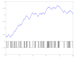
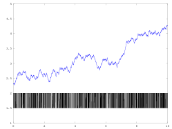
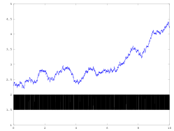
Taking $\mu=0.2$ and $\sigma=0.3$, we give sample paths of $\log(S_{t}^{\varepsilon})$ and $\alpha_{t}^{\varepsilon}$ with varying $\varepsilon$ in Figure 1. It is clear from the pictures that as $\varepsilon$ gets smaller and smaller, the fluctuation of $\alpha_{t}$ is more and more rapidly and the corresponding $S_{t}^{\varepsilon}$ approaches to a GBM.

   

(a) $\varepsilon=0.1$

(b) $\varepsilon=0.01$

(c) $\varepsilon=0.001$

Figure 1: Monte Carlo Sample Paths: $(\log(S_{t}^{\varepsilon}),\alpha_{t}^{\varepsilon})$

Example 2 (Case II).

In this example, we consider Case II with $\rho>f_{1}$ and use the following parameters

$$f_{1}=0.07,\,f_{2}=-0.03,\,\lambda_{1}=\lambda_{2}=1,\,\rho=0.10,\,K=0.01.$$

Solving the equation (27) with $x_{0}^{*}=\rho K/(\rho-f_{1})$, we have $(x^{*},x_{0}^{*})=(0.012478,0.033333)$ and $X_{0}=0.013326$. The corresponding value functions are given in Figure 2, in which $V(x,1)$ is given by the upper curve and $V(x,2)$ the lower one.

Figure 2: Value Functions $v(x,1)$ and $v(x,2)$

Example 3 (Model Calibration and a Market Test).

First we give a model calibration method. We consider

$$f_{1}=\mu+\sigma_{1}\mbox{ and }f_{2}=\mu+\sigma_{2},$$

with $\nu_{1}\sigma_{1}-\nu_{2}\sigma_{2}=0$. Given $T$, let $Y_{t}=\log(S_{t}/S_{0})=\int_{0}^{t}f(\alpha_{s})ds$, $0\leq t\leq T$. Then, $\mu$ can be approximated by $Y_{T}/T$. To estimate $\sigma_{1}$ and $\sigma_{2}$, given step size $\delta>0$, let $n\delta=T$,

$$\Delta Z_{k}=\log(S_{(k+1)\delta})-\log(S_{k\delta}),\mbox{ for }k=0,1,2,\ldots,n,$$

and $\overline{Z}=\left(\sum_{k=0}^{n-1}\Delta Z_{k}\right)/n$. Then, $\overline{Z}\approx\delta\mu$. In addition, using Yin an Zhang [16, Theorem 5.9], we can show

$$E\left(\Delta Z_{k}-\overline{Z}\right)^{2}\approx\delta\left(\frac{2\lambda_{1}\lambda_{2}(\sigma_{1}+\sigma_{2})^{2}}{(\lambda_{1}+\lambda_{2})^{3}}\right).$$

Let

$$\sigma_{0}^{2}=\frac{\sum_{k=0}^{n-1}(\Delta Z_{k}-\overline{Z})^{2}}{n-1}.$$

Then, by the Law of Large Numbers, we have

$$\sigma_{0}^{2}\approx\delta\left(\frac{2\lambda_{1}\lambda_{2}(\sigma_{1}+\sigma_{2})^{2}}{(\lambda_{1}+\lambda_{2})^{3}}\right).$$

Using $\nu_{1}\sigma_{1}=\nu_{2}\sigma_{2}$, we have

$$\sigma_{1}=\frac{\sigma_{0}}{\sqrt{\delta}}\sqrt{\frac{\lambda_{1}(\lambda_{1}+\lambda_{2})}{2\lambda_{2}}}\mbox{ and }\sigma_{2}=\frac{\sigma_{0}}{\sqrt{\delta}}\sqrt{\frac{\lambda_{2}(\lambda_{1}+\lambda_{2})}{2\lambda_{1}}},$$

Finally, we estimate $\lambda_{1}$ and $\lambda_{2}$. Let $R=\nu_{1}/\nu_{2}$. Then, $\lambda_{2}=R\lambda_{1}$.

$$\begin{array}[]{l}R_{1}=\#\{k:\,\Delta Z_{k}<0\mbox{ and }\Delta Z_{k+1}\geq 0\},\\ R_{2}=\#\{k:\,\Delta Z_{k}>0\mbox{ and }\Delta Z_{k+1}\leq 0\}.\\ \end{array}$$

Then, it follows that

$$\frac{R_{1}}{\lambda_{1}}+\frac{R_{2}}{\lambda_{2}}=T.$$

Therefore, the jump rates are given by

$$\left\{\begin{array}[]{l}\displaystyle\lambda_{1}=\frac{1}{T}\left(R_{1}+\frac{R_{2}}{R}\right),\\ \displaystyle\lambda_{2}=\frac{1}{T}\left(RR_{1}+R_{2}\right).\\ \end{array}\right.$$

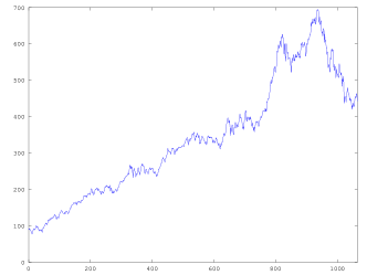
We test our selling rules using Apple Inc. (AAPL) daily closing prices during 2009/1/2 and 2013/3/28, sse Figure 3 (a). Suppose we owned 100 AAPL shares at the beginning of 2009. We evaluate at the end of each half year during this period based on that half year stock prices to determine if we should sell the shares in the near future.

We assume the risk free rate to be $\rho=0.03$ and transaction cost $K=0.01$. We use the calibration method discussed earlier and obtain the following results.

Periods	$f_{1}$	$f_{2}$	$\lambda_{1}$	$\lambda_{2}$	$\Phi(0.03)$
1st half of 2009	10.45	-10.61	100.48	124.23	-336.06
2nd half of 2009	3.21	-2.32	102.15	141.44	-217.41
1st half of 2010	3.06	-3.15	97.98	127.02	-83.18
2nd half of 2010	2.27	-1.92	103.57	134.25	-103.09
1st half of 2011	1.80	-1.85	117.19	125.00	-5.02
2nd half of 2011	3.01	-2.72	97.98	107.95	-60.56
1st half of 2012	5.39	-4.80	108.21	127.19	-185.32
2nd half of 2012	4.89	-5.13	135.25	130.95	35.79

Table 1. Parameter Values at the End of Each Period

Note that in all periods $\rho\leq f_{1}$. Therefore, only Case I applies in this example. In Table 1, we should hold through the next half year if $\Phi(0.03)\leq 0$ and sell (following our selling rule) if $\Phi(0.03)>0$. Clearly, a selling decision has to be made at the end of 2012. Using the parameter values $f_{1}=4.89$, $f_{2}=-5.13$, $\lambda_{1}=135.25$, and $\lambda_{2}=130.95$, we obtain $x^{*}=0.017213$ and the corresponding value functions $v(x,i)=V(x,i)$, $i=1,2$, which are plotted in Figure 3 (b). Therefore, one should sell as soon as $\alpha_{t}$ turns to $2$ after the new year. This occurs on the second trading day (January 3) of 2013. The shares should be sold at the close of that day at $542.10/share. As can be seen in this example, our selling rule helps to achieve the goal of letting your profits run and cutting your losses short.

 

(a) AAPL (2009/1/2–2013/3/28)

(b) Value Functions

Figure 3: Apple Inc. Daily Closes and Value Functions $v(x,1)$ and $v(x,2)$

5 Conclusion

In this paper, we considered an optimal stock selling rule under a Markov chain model. The model is natural for financial markets due to its simple structure and the solutions obtained are intuitive and easy to implement.

It would be interesting to consider more general models with multi-scale structure as treated in Yin and Zhang [16] so as to capture both long-term and short-term market movements. Such extension and related optimization problems could be subjects of future studies.

6 Appendix

Lemma 1

. Under the assumption $\Phi(\rho)>0$, the bigger root of (4) $\beta_{2}>1$.

Proof. Recall the definition of $D_{1}$ and $D_{2}$ given in (3). It is easy to check $\Phi(\rho)>0$ implies

$$D_{2}>D_{1}-f_{1}f_{2}.$$

This leads to

$$\sqrt{D_{1}-4f_{1}f_{2}D_{2}}>D_{1}-2f_{1}f_{2}.$$

Therefore, we have $\beta_{2}>1$. $\Box$

Lemma 2

. Let $\kappa_{2}={(\rho+\lambda_{1}-f_{1}\beta_{2})}/{\lambda_{1}}$, where $\beta_{2}$ is given in (5). Then, $0<\kappa_{2}<1$.

Proof. To see $\kappa_{2}>0$, it suffices to show $\rho+\lambda_{1}>f_{1}\beta_{2}$. Recall that $f_{2}<0$. We only need to show $2(\rho+\lambda_{1})f_{2}<D_{1}-\sqrt{D_{1}^{2}-4f_{1}f_{2}D_{2}}$, with $D_{1}$ and $D_{2}$ given in (3).

This is equivalent to

$$\sqrt{D_{1}^{2}-4f_{1}f_{2}D_{2}}<D_{1}-2(\rho+\lambda_{1})f_{2}.$$ (29)

It is easy to check $D_{1}-2(\rho+\lambda_{1})f_{2}=(\rho+\lambda_{2})f_{1}-(\rho+\lambda_{1})f_{2}>0$. Square both sides of (29) to obtain

$$D_{1}^{2}-4f_{1}f_{2}D_{2}<D_{1}^{2}-4(\rho+\lambda_{1})f_{2}D_{1}+4((\rho+\lambda_{1})f_{2})^{2}.$$

Simplify this inequality to obtain

$$D_{2}<(\rho+\lambda_{1})(\rho+\lambda_{2}).$$

This clearly holds. Therefore, $\kappa_{2}>0$.

Similarly, to show $\kappa_{2}<1$, it suffices to show $\rho<f_{1}\beta_{2}$. This is equivalent to

$$\sqrt{D_{1}^{2}-4f_{1}f_{2}D_{2}}>D_{1}-2\rho f_{2}.$$

Square and simplify to obtain $\rho\lambda_{1}f_{1}>\rho\lambda_{1}f_{2}$. This holds because $f_{1}>0$ and $f_{2}<0$. $\Box$

Lemma 3

. Under $\rho>f_{1}$, we have

$$\frac{K\beta_{2}}{\beta_{2}-1}<\frac{\rho K}{\rho-f_{1}}.$$

Proof. It is easy to see this inequality is equivalent to $f_{1}\beta_{2}>\rho$. Using the definition of $\beta_{2}$ and noting that $f_{2}<0$, we have

$$\sqrt{D_{1}^{2}-4f_{1}f_{2}D_{2}}>D_{1}-2\rho f_{2}.$$

If $D_{1}-2\rho f_{2}<0$, then we are done. Otherwise, square both sides to obtain

$$D_{1}^{2}-4f_{1}f_{2}D_{2}>D_{1}^{2}-4\rho f_{2}D_{1}+4\rho^{2}f_{2}^{2}.$$

Simplify this inequality to have

$$\rho\lambda_{1}f_{1}>\rho\lambda_{1}f_{2},$$

which clearly holds because $f_{1}>0$ and $f_{2}<0$.

Lemma 4

. Under $\rho>f_{1}$, we have

$$\lambda_{2}-\kappa_{2}(\rho+\lambda_{2}-f_{2})>0,\\$$ (30)

which implies $\lambda_{2}-\kappa_{2}(\rho+\lambda_{2})>0$.

Proof. Let $H_{0}=\rho+\lambda_{2}-f_{2}>0$. Using the definition of $\kappa_{2}$, (30) is equivalent to

$$H_{0}(\rho+\lambda_{1}-f_{1}\beta_{2})<\lambda_{1}\lambda_{2}.$$

Therefore, we have

$$(\rho+\lambda_{1})H_{0}-\left(\frac{D_{1}-\sqrt{D_{1}^{2}-4f_{1}f_{2}D_{2}}}{2f_{2}}\right)H_{0}<\lambda_{1}\lambda_{2}.$$

Multiply both sides by $(2f_{2})$ and rearrange the terms to obtain

$$H_{0}\sqrt{D_{1}^{2}-4f_{1}f_{2}D_{2}}>H_{0}D_{1}-2f_{2}[(\rho+f_{1})H_{0}-\lambda_{1}\lambda_{2}].$$

Square both sides and simplify to have

$$(\rho+\lambda_{1}-f_{1})H_{0}-\lambda_{1}\lambda_{2}>0,$$

which is exactly the assumption $\phi(\rho)>0$. This completes the proof. $\Box$

References

- [1] B.R. Barmish and J.A. Primbs, On market-neutral stock trading arbitrage via linear feedback, Proc. American Control Conference, Montreal, 2012.
- [2] D. Duffie, Dynamic Asset Pricing Theory, 2nd Ed., Princeton University Press, Princeton, NJ, 1996.
- [3] R. J. Elliott and P. E. Kopp, Mathematics of Financial Markets, Springer-Verlag, New York, 1998.
- [4] J.P. Fouque, G. Papanicolaou, and R.K. Sircar, Derivatives in Financial Markets with Stochastic Volatility, Cambridge University Press, 2000.
- [5] X. Guo and Q. Zhang, Optimal selling rules in a regime switching model, IEEE Transactions on Automatic Control, Vol. 50, pp. 1450-1455, (2005).
- [6] K. Helmes, Computing optimal selling rules for stocks using linear programming, Mathematics of Finance, G. Yin and Q. Zhang, (Eds), Contemporary Mathematics, American Mathematical Society, pp. 187-198, (2004).
- [7] J. C. Hull, Options, Futures, and Other Derivatives, 3rd Ed., Prentice Hall, Upper Saddle River, NJ, 1997.
- [8] I. Karatzas and S. E. Shreve, Methods of Mathematical Finance, Springer, New York, 1998.
- [9] A. Lkka and M. Zervos, Long-term optimal real investment strategies in the presence of adjustment costs, preprint, (2007).
- [10] A. Merhi and M. Zervos, A model for reversible investment capacity expansion, SIAM J. Contr. Optim., Vol. 46, pp. 839-876, (2007).
- [11] M. Musiela and M. Rutkowski, Martingale Methods in Financial Modeling, Springer, New York, 1997.
- [12] R. Norberg, The Markov chain market, ASTIN Bulletin, Vol. 33, pp. 265-287, (2003).
- [13] B. ksendal, Stochastic Differential Equations, 6th Ed., Springer-Verlag, New York, 2003.
- [14] J. van der Hoek and R.J. Elliott, American option prices in a Markov chain market model, Applied Stochastic Models in Business and Industry, Vol. 28, pp. 35–59, (2012).
- [15] G. Yin, R.H. Liu, and Q. Zhang, Recursive algorithms for stock Liquidation: A stochastic optimization approach, SIAM J. on Optimization, Vol. 13 (2002), 240-263.
- [16] G. Yin and Q. Zhang, Continuous-Time Markov Chains and Applications, A Two-Time-Scale Approach, 2nd Ed, Springer, New York, 2013.
- [17] H. Zhang and Q. Zhang, Trading a mean-reverting asset: Buy low and sell high, Automatica, Vol. 44, pp. 1511-1518, (2008).
- [18] Q. Zhang, Stock trading: An optimal selling rule, SIAM J. on Control and Optimization, Vol. 40, pp. 64-87, (2001).