The achievable performance of convex demixing

Abstract.

Demixing is the problem of identifying multiple structured signals from a superimposed, undersampled, and noisy observation. This work analyzes a general framework, based on convex optimization, for solving demixing problems. When the constituent signals follow a generic incoherence model, this analysis leads to precise recovery guarantees. These results admit an attractive interpretation: each signal possesses an intrinsic degrees-of-freedom parameter, and demixing can succeed if and only if the dimension of the observation exceeds the total degrees of freedom present in the observation.

1 Introduction

Demixing refers to the problem of extracting multiple informative signals from a single, possibly noisy and undersampled, observation. One rather general model for a mixed observation $\bm{z}_{0}\in\mathbb{R}^{m}$ takes the form

$$\bm{z}_{0}=\bm{A}\mathopen{}\mathclose{{}\left(\sum\nolimits_{i=1}^{n}\bm{U}_{i}\bm{x}_{i}^{\smash{\natural}}+\bm{w}}\right),$$ (1.1)

where the constituents $(\bm{x}_{i}^{\smash{\natural}})_{i=1}^{n}$ are the unknown informative signals that we wish to find; the matrices $(\bm{U}_{i})_{i=1}^{n}$ model the relative orientation of the constituent vectors; the operator $\bm{A}\in\mathbb{R}^{m\times d}$ compresses the observation from $d$ dimensions to $m\leq d$ dimensions; and $\bm{w}\in\mathbb{R}$ is unstructured noise. We assume that all elements appearing in (1.1) are known except for the constituents $(\bm{x}_{i}^{\smash{\natural}})_{i=1}^{n}$ and the noise $\bm{w}$.

Numerous applications of the model (1.1) appear in modern data-intensive science. In imaging, for example, the informative signals can model features like stars and galaxies [SDC03], while an undersampling operator accounts for known occlusions or missing data [ESQD05a, SKPB12]. In graphical model selection, the data may consist of the sum of a sparse component that encodes causality structure and a confounding low-rank component that arises from unobserved latent variables [CPW10]. Similar mixed-signal models appear in robust statistics [CLMW11, CJSC13] and image processing [PGW⁺12, WGMM13]. In every case, the question of interest is

When is it possible to recover the constituents from the observation?

This work answers this question for a popular class of demixing procedures under a random model. The analysis reveals that each constituent possesses a degrees-of-freedom parameter, and that these demixing procedures can succeed with high probability if and only if the total number of measurements exceeds the total degrees of freedom.

In the next two subsections, we describe a well-known recipe that converts a priori structural information on the constituents $\bm{x}_{i}^{\smash{\natural}}$ into an convex optimization program suited for demixing (1.1). Section 1.3 motivates a random model that we use to study demixing, and Section 1.4 defines the degrees-of-freedom parameter $\delta_{i}$. The main result appears in Section 1.5.

1.1 Structured signals and convex penalties

In the absence of assumptions, it is impossible to reliably recover unknown vectors from a superposition of the form (1.1). In order to have any hope of success, we must make use of domain-specific knowledge about the types of constituents making up our observation. This knowledge often implies that our constituents belong to some set of highly-structured elements. Typical examples of these structured families include sparse vectors and low-rank matrices.

Sparse vectors

A sparse vector has many entries equal to zero. Sparse vectors regularly appear in modern signal and data processing applications for a variety of reasons. Bandlimited communications signals, for example, are engineered to be sparse in the frequency domain. The adjacency matrix of a sparse graph is sparse by definition. Piecewise smooth functions are nearly sparse in wavelet bases, so that many natural images exhibit sparsity in the wavelet domain [Mal09, Sec. 9].

Low-rank matrices

A matrix has low rank if many of its singular values are equal to zero. Low-rank structure appears whenever the rows or columns of a matrix satisfy many nontrivial linear relationships. For example, strong correlations between predictors cause many statistical datasets to exhibit low-rank structure. Rank deficient matrices appear in a number of other areas, including control theory [Faz02, Sec. 6], video processing [CLMW11], and structured images [PGW⁺12].

Other types of structured families that appear in the literature include the family of sign vectors $\{\pm 1\}^{d}\subset\mathbb{R}$ [MR11], nonnegative sparse vectors [DT10], block- and group-sparse vectors and matrices [RKD98, MÇW03], and orthogonal matrices [CRPW12].

In each of these cases, the structured family possesses an associated convex function that, roughly speaking, measures the amount of complexity of a signal with respect to the family [DT96, Tem03, CRPW12]. For sparse vectors and low-rank matrices, the natural penalty functions are the $\ell_{1}$ norm and the Schatten 1-norm:

$$\mathopen{}\mathclose{{}\left\|{\bm{x}}}\right\|_{{\ell_{1}}\!}:=\sum\nolimits_{i=1}^{d}\mathopen{}\mathclose{{}\left|{x_{i}}}\right|\quad\text{and}\quad\mathopen{}\mathclose{{}\left\|{\bm{X}}}\right\|_{S_{1}}:=\sum\nolimits_{i=1}^{p\wedge q}\sigma_{i}(\bm{X}),$$

where $\sigma_{i}(\bm{X})$ is the $i$th singular value of $\bm{X}$ and the wedge $\wedge$ denotes the minimum of two numbers. See [CRPW12, Sec. 2.2] for additional examples as well as a principled approach to constructing convex penalty functions. These convex complexity measures form the building blocks of the demixing procedures that we study in this work.

1.2 A generic demixing framework

Given an observation of the form (1.1), we desire a computational method for recovering the constituents $\bm{x}_{i}^{\smash{\natural}}$. We now describe a well-known framework that combines convex complexity measures into a convex optimization program that demixes a signal. Specific instances of this recipe appear in numerous works [DH01, CSPW09, CJSC13, PGW⁺12], and the general format described below is closely related to the work [MT12, WGMM13].

Assume that, for each constituent $\bm{x}_{i}^{\smash{\natural}}$, we have determined an appropriate convex complexity function $f_{i}$. For example, if we suspect that the $i$th constituent $\bm{x}_{i}^{\smash{\natural}}$ is sparse, we may choose the $f_{i}=\mathopen{}\mathclose{{}\left\|{\cdot}}\right\|_{{\ell_{1}}\!}$, the $\ell_{1}$ norm. In the Lagrange formulation of the demixing procedure, we combine the regularizers into a single master penalty function $F_{\bm{\lambda}}\colon(\mathbb{R})^{n}\to\mathbb{R}$ given by

$$F_{\bm{\lambda}}(\bm{x}_{1},\dotsc,\bm{x}_{n-1},\bm{x}_{n}):=\sum\nolimits_{i=1}^{n}\lambda_{i}f_{i}(\bm{x}_{i}),$$

where the weights $\lambda_{i}>0$. In this formulation, we minimize the master penalty $F_{\bm{\lambda}}$ plus a Euclidean-norm penalty constraint that ensures consistency with our observation:

$$\operatorname*{minimize}_{\bm{x}_{i}\in\mathbb{R}}\;F_{\bm{\lambda}}(\bm{x}_{1},\dotsc,\bm{x}_{n-1},\bm{x}_{n})+\mathopen{}\mathclose{{}\left\|{\bm{A}^{\dagger}\mathopen{}\mathclose{{}\left[\bm{A}\mathopen{}\mathclose{{}\left(\sum\nolimits_{i=1}^{n}\bm{U}_{i}\bm{x}_{i}}\right)-\bm{z}_{0}}\right]}}\right\|^{2}$$ (1.2)

where $\mathopen{}\mathclose{{}\left\|{\bm{x}}}\right\|^{2}:=\langle\bm{x},\bm{x}\rangle$ is the squared Euclidean norm. We include the Moore–Penrose pseudoinverse $\bm{A}^{\dagger}$ in the consistency term to ensure that our recovery procedure is independent of the conditioning of $\bm{A}$. This demixing procedure succeeds when an optimal point $(\tilde{\bm{x}}_{i})_{i=1}^{n}$ of (1.2) provides a good approximation for the true constituents $(\bm{x}_{i}^{\smash{\natural}})_{i=1}^{n}$.

Rather than restrict ourselves to specific choices of Lagrange parameters $\bm{\lambda}$, we study whether it is possible to demix the constituents of $\bm{z}_{0}$ using a method of the form (1.2) for the best choice of weights $\bm{\lambda}$. To study this setting, we focus our analysis on the more powerful constrained formulation of demixing:

$$\operatorname*{minimize}_{\bm{x}_{i}\in\mathbb{R}} \mathopen{}\mathclose{{}\left\|{\bm{A}^{\dagger}\mathopen{}\mathclose{{}\left(\bm{A}\sum\nolimits_{i=1}^{n}\bm{U}_{i}\bm{x}_{i}-\bm{z}_{0}}\right)}}\right\|^{2}$$ (1.3)

   subject to $$f_{i}(\bm{x}_{i})\leq f_{i}(\bm{x}_{i}^{\smash{\natural}})\quad\text{for each}\quad i=1,\dotsc,n-1,n.$$

The theory of Lagrange multipliers indicates that solving the constrained demixing program (1.3) is essentially equivalent to solving the Lagrange problem (1.2) with the best choice of weights $\bm{\lambda}$. There are some subtle issues in this equivalence, notably the fact that (1.2) can have strictly more optimal points than the corresponding constrained problem (1.3). We refer to [Roc70, Sec. 28] for further details.

We wish to interrogate whether an optimal point $(\hat{\bm{x}}_{i})_{i=1}^{n}$ of (1.3) forms a good approximation for the true constituents $(\bm{x}_{i}^{\smash{\natural}})_{i=1}^{n}$. For this study, we distinguish two situations.

Exact recovery

In the noiseless setting where $\bm{w}=\bm{0}$, can we guarantee that the constrained demixing program (1.3) recovers the constituents exactly?

Stable recovery

For nonzero noise $\bm{w}\neq\bm{0}$, can we guarantee that any solution to the constrained demixing problem (1.3) provides a good approximation to the constituents $\bm{x}_{i}^{\smash{\natural}}$?

The following definition makes these notions precise.

Definition 1.1 (Exact and stable recovery).

We say that exact recovery is achievable in (1.3) if the tuple $(\bm{x}_{i}^{\smash{\natural}})_{i=1}^{n}$ is the unique optimal point of (1.3) when $\bm{w}=\bm{0}$. We say that stable recovery is achievable if there exists number $C>0$, such that for any optimal point $(\hat{\bm{x}}_{i})_{i=1}^{n}$ of (1.3), we have

$$\mathopen{}\mathclose{{}\left\|{\hat{\bm{x}}_{i}-\bm{x}_{i}^{\smash{\natural}}}}\right\|\leq C\mathopen{}\mathclose{{}\left\|{\bm{w}}}\right\|\quad\text{for all}\quad i=1,\dotsc,n-1,n.$$ (1.4)

The value of $C$ may depend on all problem parameters except $\bm{w}$.

The goal of this work is to describe when exact and stable recovery are achievable for the constrained demixing program (1.3).

1.3 A generic model for incoherence

A necessary requirement to identify signals from a superimposed observation is that the constituent signals must look different. The superposition of two sparse vectors, for example, is still sparse; a priori knowledge that both vectors are sparse provides little guidance in determining how to allocate the nonzero elements between the two constituents. On the other hand, a sparse vector looks very different from a superposition of a small number of sinusoids. This structural diversity makes distinguishing spikes from sines tractable [Tro08]. We extend this idea to more general families by saying that structured vectors that look very different from one another are incoherent.

In this work, we follow [DH01, MT12] and model incoherence by assuming that the families are randomly oriented relative to one another. The set of all possible orientations on $\mathbb{R}$ is the orthogonal group $\mathsf{O}_{d}$ consisting of all $d\times d$ orthogonal matrices:

$$\mathsf{O}_{d}:=\bigl{\{}\bm{U}\in\mathbb{R}^{d\times d}\mathrel{\mathop{:}}\bm{U}^{t}\bm{U}=\mathbf{I}\bigr{\}}.$$

The orthogonal group is a compact group, and so it possesses a unique invariant probability measure called the Haar measure [Fre06, Ch. 44]. We model incoherence among the constituents $\bm{x}_{i}^{\smash{\natural}}$ by drawing the orientations $\bm{U}_{i}$ from the Haar measure.

Definition 1.2 (Random orientation model).

We say that the matrices $(\bm{U}_{i})_{i=1}^{d}$ satisfy the random orientation model if the matrices $\bm{U}_{1},\dotsc,\bm{U}_{n-1},\bm{U}_{n}$ are drawn independently from the Haar measure on $\mathsf{O}_{d}$.

The random orientation model is analogous to random measurements models that appear in the compressed sensing literature [CT05, Don06]. In this work, however, we find that orienting the structures randomly through the rotations $\bm{U}_{i}$ provides sufficient randomness for the analysis. We have no need to assume that the measurement matrix $\bm{A}$ is random.

1.4 Descent cones and the statistical dimension

Our study of the exact and stable recovery capabilities of the constrained demixing program (1.3) relies on a geometric analysis of the optimality conditions of the convex program (1.3). The key player in this analysis is the following cone that captures the local behavior of a convex function at a point (Figure 1).

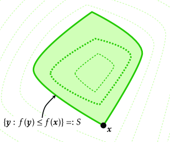
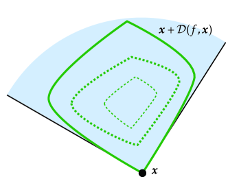
Figure 1: Descent cone. [Left] The sublevel set $S$ (shaded) of a convex function $f$ (level lines) at a point $\bm{x}$. [Right] The descent cone $\mathcal{D}(f,\bm{x})$ (shaded) is the cone generated by $S$ at $\bm{x}$.

Definition 1.3 (Descent cone).

The descent cone $\mathcal{D}(f,\bm{x})$ of a convex function $f$ at a point $\bm{x}$ is the cone generated by the perturbations about $\bm{x}$ that do not increase $f$:

$$\mathcal{D}(f,\bm{x}):=\{\bm{y}\mathrel{\mathop{:}}f(\bm{x}+\tau\bm{y})\leq f(\bm{x})\text{ for some }\tau>0\}.$$ (1.5)

Intuitively, a convex penalty function $f$ will be more effective at finding a structured vector $\bm{x}^{\smash{\natural}}$ if most perturbations around $\bm{x}^{\smash{\natural}}$ increase the value of $f$, i.e., if the descent cone $\mathcal{D}(f,\bm{x}^{\smash{\natural}})$ is small. Our next definition provides a summary parameter that lets us quantify the size of a convex cone.

Definition 1.4 (Statistical dimension).

Let $C\subset\mathbb{R}$ be a closed convex cone, and define the Euclidean projection $\bm{\Pi}_{C}\colon\mathbb{R}\to C$ onto $C$ by

$$\bm{\Pi}_{C}(\bm{x}):=\operatorname*{arg\;min}_{\bm{y}\in C}\mathopen{}\mathclose{{}\left\|{\bm{y}-\bm{x}}}\right\|^{2}.$$

The statistical dimension $\delta(C)$ of $C$ is given by the average value

$$\delta(C):=\operatorname{\mathbb{E}}_{\bm{g}}\mathopen{}\mathclose{{}\left[\mathopen{}\mathclose{{}\left\|{\bm{\Pi}_{C}(\bm{g})}}\right\|^{2}}\right],$$ (1.6)

where $\bm{g}\sim\mathrm{N}(\bm{0},\mathbf{I})$ is a standard Gaussian vector.

The statistical dimension satisfies a number of properties that make it an appropriate measure of the “size” or “dimension” of a convex cone. It also extends a number of useful properties for the usual dimension of a linear subspace to convex cones [ALMT13, Sec. 4]. Moreover, a number of calculations for the statistical dimension are available in the literature [SPH09, CRPW12, ALMT13, FM13], which makes the statistical dimension an appealing parameter in practice.

The statistical dimension turns out to be the key parameter which determines the success and failure of demixing under the random orientation model. To shorten notation, we abbreviate the statistical dimensions of the descent cones $\mathcal{D}(f_{i},\bm{x}_{i}^{\smash{\natural}})$:

$$\delta_{i}:=\delta_{i}\Bigl{(}\overline{\mathcal{D}(f_{i},\bm{x}_{i}^{\smash{\natural}})}\Bigr{)}\quad\text{for}\quad i=1,\dotsc,n-1,n,$$ (1.7)

where the overline denotes the closure.

1.5 Main result

We are now in a position to state our main result.

Theorem A.

With $\delta_{i}$ as in (1.7), define the total dimension $\Delta$ and the scale $\sigma$ by

$$\Delta:=\sum\nolimits_{i=1}^{n}\delta_{i}\quad\text{and}\quad\sigma:=\sqrt{\sum\nolimits_{i=1}^{n}\delta_{i}\wedge(d-\delta_{i})}.$$ (1.8)

Choose a probability tolerance $\eta\in(0,1)$, and define the transition width

$$\lambda_{*}:=\tfrac{4}{3}\log\mathopen{}\mathclose{{}\left(\tfrac{1}{\eta}}\right)+2\sigma\sqrt{\log\mathopen{}\mathclose{{}\left(\tfrac{1}{\eta}}\right)}.$$ (1.9)

Suppose that the matrices $(\bm{U}_{i})_{i=1}^{n}$ are drawn from the random orientation model and that the measurement operator $\bm{A}\in\mathbb{R}^{m\times n}$ has full row rank. Then

$$m\geq\Delta+\lambda_{*} \implies\text{stability is achievable with probability}\geq 1-\eta;$$ (1.10)

$$m\leq\Delta-\lambda_{*} \implies\text{exact recovery is achievable with probability}\leq\eta,$$ (1.11)

where we define exact and stable recovery in Definition 1.1.

Theorem A provides detailed information about the capability of constrained demixing (1.3) under the random orientation model.

Phase transition

The capability of (1.3) changes rapidly when the number of measurements $m$ passes through the total statistical dimension $\Delta$. For $m$ somewhat less than $\Delta$, exact recovery is highly unlikely. On the other hand, when $m$ is a bit larger than $\Delta$, we have stable recovery with high probability. This justifies our heuristic that the number of measurements required for demixing is equal to the total statistical dimension.

Transition width

Theorem A tightly controls the width of the transition region between success and failure. When the probability tolerance $\eta$ is independent of $d$ and $n$, the transition width satisfies

$$\lambda_{*}=O(\sigma)=O\bigl{(}\sqrt{nd}\bigr{)}\quad\text{as}\quad d\to\infty.$$ (1.12)

The second equality follows from the observation that $\sigma^{2}\leq nd$ because the statistical dimension is never larger than the ambient dimension (cf. [ALMT13, Sec. 4]). In many applications, the number $n$ of constituents is independent of the ambient dimension, so the transition between success and failure occurs over no more than $O(\sqrt{d})$ measurements as $d\to\infty$.

Strong probability bounds

Probability tolerances $\eta$ that decay rapidly with the ambient dimension $d$ can provide strong guarantees for demixing [MT12, Sec. 4.3]. For example, when the number of measurements $m\geq\Delta+cd$ for some $c>0$, Theorem A guarantees that

$$\text{\emph{Stability is achievable with probability}}\geq 1-\mathrm{e}^{-c^{\prime}d}.$$

Due to the estimate $\sigma^{2}\leq nd$ from above, the constant $c^{\prime}>0$ need depend only on $c$ and $n$. Such exponentially small failure probabilities lead to strong demixing bounds using union-bound arguments as in [MT12, Secs. 6.1.1 & 6.2.2]. We omit the details for brevity.

Extreme demixing

How many constituents can we reliably demix? The answer is simple:

Theorem A allows $$n d$$ proportional to .

Consider, for example, the fully observed case $m=d$, and fix a probability of success $\eta$ independent of $d$. Suppose that $\Delta\leq(1-\varepsilon)d$ for some $\varepsilon>0$. For demixing to succeed, by Theorem A, we only need

$$d-\Delta\geq\varepsilon d\geq\lambda_{*}=O(\sqrt{nd})\quad\text{as}\quad d\to\infty$$

where the equality is (1.12). Thus, the implication (1.10) remains nontrivial as $d\to\infty$ so long as $n\leq cd$ for some sufficiently small $c>0$.

This growth regime is essentially optimal. It can be shown that $\delta_{i}\geq 1/2$ whenever $\bm{x}_{i}^{\smash{\natural}}$ is not the unique global minimum of $f_{i}$. Thus, excepting trivial situations, we have $\Delta\geq n/2$, so that when $n\gtrsim 2d$, demixing must fail with high probability by (1.11).

The proof of Theorem A is based on a geometric optimality condition for the constrained demixing program (1.3) that characterizes exact and stable recovery in terms of a configuration of randomly oriented convex cones. A new extension of the approximate kinematic formula from [ALMT13] lets us provide precise bounds on the probability that this geometric optimality condition holds under the random orientation model.

1.6 Outline

Section 2 describes the related work on demixing. The proof of Theorem A appears in Section 3. Section 4 provides two simple numerical experiments that illustrate the accuracy of Theorem A, and we conclude in Section 5 with some open problems. The technical details in our development appear in the appendices.

1.7 Notation and basic facts

Vectors appear in bold lowercase, while matrices are bold and capitalized. The range and nullspace of a matrix $\bm{X}$ are $\mathcal{R}(\bm{X})$ and $\mathcal{N}(\bm{X})$. The Minkowski sum of sets $S_{1},S_{2}\subset\mathbb{R}$ is $S_{1}+S_{2}$. When more than two sets are involved, we define the Minkowski sum $\sum_{i}S_{i}$ inductively. We write $-S$ for the reflection of $S$ about $\bm{0}$ and $\overline{S}$ for the closure of $S$.

A convex cone $C\subset\mathbb{R}$ is a convex set that is positive homogeneous: $\bm{x},\bm{y}\in C\implies\lambda(\bm{x}+\bm{y})\in C$ for all $\lambda>0$. All cones in this work contain the origin $\bm{0}$. We write $\mathcal{C}_{d}$ for the set of all closed, convex cones in $\mathbb{R}$. For any cone $C\subset\mathbb{R}$, we define the polar cone $C^{\circ}\in\mathcal{C}_{d}$ by

$$C^{\circ}:=\{\bm{y}\in\mathbb{R}\mathrel{\mathop{:}}\langle\bm{x},\bm{y}\rangle\leq 0\quad\text{for all}\quad\bm{x}\in C\}.$$ (1.13)

The bipolar formula states $C^{\circ\circ}=\overline{C}$. We measure the distance between two cones $C,D\subset\mathbb{R}$ by computing the maximal inner product

$$\llangle C,D\rrangle:=\sup_{\begin{subarray}{c}\bm{x}\in C\cap\mathsf{B}_{d}\\ \bm{y}\in D\cap\mathsf{B}_{d}\end{subarray}}\langle\bm{x},\bm{y}\rangle.$$ (1.14)

It follows from the Cauchy–Schwarz inequality that $\llangle C,D\rrangle\leq 1$ for every pair of cones, while the equality conditions for Cauchy–Schwarz show that $\llangle C,D\rrangle=1$ if and only if the intersection $\overline{C}\cap\overline{D}$ contains a ray.

We will refer to the following elementary properties of the statistical dimension. For any closed convex cones $C\in\mathcal{C}_{d}$ and $D\in\mathcal{C}_{d^{\prime}}$, the statistical dimension reverses under polarity

$$\delta(C^{\circ})=d-\delta(C)$$ (1.15)

and splits under the Cartesian product

$$\delta(C\times D)=\delta(C)+\delta(D).$$ (1.16)

Simple proofs of relations (1.15) and (1.16) appear in [ALMT13, Sec. 4].

2 Context and related work

This work is a successor to the author’s earlier work [MT12] on demixing with $n=2$ components in the fully observed $m=d$ setting. The techniques used in this paper hail from [ALMT13], which studied phase transitions in randomized optimization programs. While those two works are the closest in spirit to our development below, numerous works on demixing appear in the literature. This section provides an overview of the literature on demixing, from its origins in sparse approximation to recent developments towards a general theory.

Demixing and sparse approximation.

Early work on demixing methods used the $\ell_{1}$ norm to encourage sparsity. Taylor, Banks, & McCoy [TBM79] used (1.2) with $f_{1}=f_{2}=\mathopen{}\mathclose{{}\left\|{\cdot}}\right\|_{{\ell_{1}}\!}$ to demix a sparse signal from sparse noise, with applications to geophysics. About ten years later, Donoho & Stark [DS89] explained how uncertainty principles can guarantee the success of demixing signals that are sparse in frequency from those that are sparse in time using the $\ell_{1}$ norm.

The analysis of Donoho & Huo [DH01] provided incoherence-based guarantees which demonstrate that exact recovery is possible under fairly generic conditions. This work motivated interest in morphological component analysis (MCA) for image processing [SDC03, ESQD05b, BMS06, BSFM07, BSF⁺07]. MCA posits that images are the superposition of a small number of signals from a known dictionary—such as pointillistic stars and wispy galaxies. Demixing with the $\ell_{1}$ norm provides a computational framework for decomposing these images into their constituent signals.

A number of recent papers provide theoretical guarantees for demixing with the $\ell_{1}$ norm. Wright & Ma showed that $\ell_{1}$-norm demixing can recovery a nearly dense vector from a sufficiently sparse corruption [WM09]. Additional work along these lines appears in [SKPB12, PBS13, NT13, Li13]. The phase transition for demixing two signals using the $\ell_{1}$-norm was first identified by the present authors in [MT12]. The very recent work [FM13] recovers similar guarantees under a slightly different model, and it also provides stability guarantees.

Demixing beyond sparsity.

Applications for mixed signal model (1.1) when the constituents satisfy more general structural assumptions appear in a number of areas. The work of Chandrasekaran et al. [CSPW09, CPW10, CSPW11] demonstrated that a demixing program of the form (1.2) can recover the superposition of a sparse and low-rank matrix. The independent work of Candès et al. [CLMW11] uses this model for robust principal component analysis and image processing applications.

Modifications to the rank-sparsity model find applications in robust statistics [XCS10, MT11, XCS12] and its compressed variants  [WGMM13, WSB11], image processing [WGMM13, PGW⁺12], and network analysis [JRSR10, JRSR11, CJSC11a, CJSC11b, CJSC13].

A general theory takes shape.

Recent work has started to unify the piecemeal results discussed above. Chandrasekaran et. al [CRPW12] gave a general treatment of the $n=1$ case using Gaussian width analysis. For the $n=2$ and $m=d$ case, the present authors used tools from integral geometry to demonstrate numerically matching upper and lower exact recovery guarantees for demixing [MT12]. The first fully rigorous account of phase transitions in demixing problems, for the $n=2$ and $m=d$ case, appeared in work of Amelunxen et al. [ALMT13].

In very recent work, Foygel & Mackey [FM13] studied the $n=2$ case with a linear undersampling model that differs slightly from the one we consider in this work. These empirically sharp results recover and extend some of the bounds in [MT12], but they do not prove that a phase transition occurs. Notably, the work of Foygel & Mackey offers guidance on the choice of Lagrange parameters.

The only previous result for the demixing setup where the number of constituents $n$ is arbitrary appears in Wright et al. [WGMM13]. Their results provide recovery guarantees for the Lagrange formulation of the undersampled demixing program (1.2) when sufficiently strong guarantees are available for the fully observed $m=d$ case. Their guarantees, however, do not identify the phase transition between success and failure.

3 Proof of the main result

This section presents the arc of the argument leading to Theorem A, but it postpones the proof of intermediate results to the appendices. Section 3.1 describes deterministic conditions for exact and stable recovery. In Section 3.2, we provide simplifications for these deterministic conditions that hold almost surely under the random orientation model. These simplifications reduce the recovery conditions to a single geometric condition involving the intersection of (polars of) randomly oriented descent cones.

Our key tool, the approximate kinematic formula, appears in Section 3.3. This formula bounds the probability that an arbitrary number of randomly oriented cones intersect in terms of the statistical dimension. It extends and refines a result of Amelunxen et al. [ALMT13, Thm. 7.1]. We complete the argument in Section 3.4 by applying the kinematic formula to our simplified geometric recovery condition.

3.1 Deterministic recovery conditions

We begin the proof of Theorem A with deterministic conditions for exact recovery and stability for the constrained demixing problem (1.3). These conditions rephrase exact recovery and stability in terms of configurations of descent cones. In order to highlight the symmetries in these conditions, we first introduce some notation that we use throughout the proof . Define

$$D_{i}:=\mathcal{D}(f_{i},\bm{x}_{i}^{\smash{\natural}})\quad\text{for}\quad i=1,\dotsc,n,\quad D_{n+1}:=\mathcal{N}(\bm{A}),\quad\text{and}\quad\bm{U}_{n+1}:=\mathbf{I}.$$ (3.1)

The exact recovery condition is the event

$$-\bm{U}_{i}D_{i}\cap\mathopen{}\mathclose{{}\left(\sum\nolimits_{j\neq i}\bm{U}_{j}D_{j}}\right)=\{\bm{0}\}\quad\text{for all}\quad i=1,\dotsc,n,n+1.$$ (ERC)

In words, the exact recovery condition requires that no descent cone shares a ray with the sum of the other cones. The stable recovery condition strengthens (ERC) by requiring that the cones are separated by some positive angle:

$$\mathopen{}\mathclose{{}\left\llangle-\bm{U}_{i}D_{i},\sum\nolimits_{j\neq i}\bm{U}_{j}D_{j}}\right\rrangle<1\quad\text{for all}\quad i=1,\dotsc,n,n+1,$$ (SRC)

where we recall the definition (1.14) of the inner product between cones. These two conditions precisely characterize exact and stable recovery for constrained demixing (1.3).

Lemma 3.1.

Success is achievable in the noiseless case if and only if the exact recovery condition (ERC) holds. If the stable recovery condition condition (SRC) holds, then stability is achievable.

We prove Lemma 3.1 in Appendix A. The proof of exact recovery is based on a perturbative argument that extends the proof [MT12, Lem. 2.3] of the recovery conditions for demixing two signals. The stable recovery result follows similar lines.

3.2 Three simplifications

Our goal in this work is the analysis of demixing when the orientations are drawn independently from the Haar measure on the orthogonal group. In this section, we describe some simplifications that arise from the fact that this measure is invariant and continuous. In the end, we reduce the problem of studying the exact and stable recovery conditions (ERC) and (SRC) hold to the problem of studying a single geometric question: What is the probability that $n+1$ randomly oriented cones share a ray?

In Section 3.2.1, we show that we can replace the deterministic nullspace $\mathcal{N}(\bm{A})$ with a randomly oriented $d-m$ dimensional subspace, which effectively randomizes the nullspace of the measurement operator $\bm{A}$. In Section 3.2.2, we find that (ERC) and (SRC) are equivalent under the random orientation model. Finally, we simplify the exact recovery condition (ERC) in Section 3.2.3.

3.2.1 Randomizing the nullspace

In definition (3.1), we fix the rotation $\bm{U}_{i}=\mathbf{I}$ in order to make the statement of the exact and stable recovery conditions symmetric. However, this symmetry is broken by the random orientation model because only $(\bm{U}_{i})_{i=1}^{n}$ are taken at random. The next result restores this symmetry.

Lemma 3.2.

Suppose that $(\bm{U}_{i})_{i=1}^{n}$ are drawn from the random orientation model and fix $\bm{U}_{n+1}=\mathbf{I}$. Let $(\bm{Q}_{i})_{i=1}^{n+1}$ be an $(n+1)$-tuple of i.i.d. random rotations. Then

$$\mathbb{P}\mathopen{}\mathclose{{}\left\{\eqref{eq:erc}\text{ holds}}\right\} =\mathbb{P}\mathopen{}\mathclose{{}\left\{-\bm{Q}_{i}D_{i}\cap\sum\nolimits_{j\neq i}\bm{Q}_{j}D_{j}=\{\bm{0}\}\text{ for each }i=1,\dotsc,n,n+1}\right\}.$$ (3.2)

Under the same conditions,

$$\mathbb{P}\mathopen{}\mathclose{{}\left\{\eqref{eq:src}\text{ holds}}\right\} =\mathbb{P}\mathopen{}\mathclose{{}\left\{\mathopen{}\mathclose{{}\left\llangle-\bm{Q}_{i}D_{i},\sum\nolimits_{j\neq i}\bm{Q}_{j}D_{j}}\right\rrangle<1\text{ for each }i=1,\dotsc,n,n+1}\right\}.$$ (3.3)

The proof, which appears in Appendix B.1, requires only an elementary application of the rotation invariance of the Haar measure.

3.2.2 Exchanging stable for exact recovery

Our second simplification shows that the stability condition (SRC) holds with the same probability that the recovery condition (ERC) holds.

Lemma 3.3.

The probabilities appearing in (3.2) and (3.3) are equal.

This result is immediate for closed cones: compactness arguments imply that two closed cones do not intersect if and only if the angle between the cones is strictly less than one. Hence, (ERC) is equivalent to (SRC) when all of the descent cones $D_{i}$ are closed. The proof of Lemma 3.3 in Appendix B.2 shows that this equivalence almost surely holds even when the cones are not closed.

3.2.3 Polarizing the exact recovery condition

Our final simplification reduces the $n+1$ intersections in (3.2) to a single intersection.

Lemma 3.4.

Suppose that $D_{i}\neq\{\bm{0}\}$ for at least two indices $i\in\{1,\dotsc,n,n+1\}$. Then

$$\mathbb{P}\mathopen{}\mathclose{{}\left\{-\bm{Q}_{i}D_{i}\cap\sum\nolimits_{j\neq i}\bm{Q}_{j}D_{j}=\{\bm{0}\}\text{ for each }i=1,\dotsc,n,n+1}\right\}\\ =\mathbb{P}\bigl{\{}\bm{Q}_{1}D_{1}^{\circ}\cap\dotsb\cap\bm{Q}_{n}D_{n}^{\circ}\cap\bm{Q}_{n+1}D_{n+1}^{\circ}\neq\{\bm{0}\}\bigr{\}}$$ (3.4)

where the matrices $(\bm{Q}_{i})_{i=1}^{n}$ are drawn i.i.d. from the random orientation model.

The demonstration appears in Appendix B.3, but we describe main difficulty here. Let $C,D\subset\mathbb{R}$ be two cones such that $-C\cap D=\{\bm{0}\}$. The separating hyperplane theorem provides a nonzero $\bm{w}\in\mathbb{R}$ that weakly separates $-C$ and $D$:

$$\langle\bm{w},-\bm{x}\rangle\geq 0\text{ for all }\bm{x}\in C\quad\text{and}\quad\langle\bm{w},\bm{y}\rangle\leq 0\text{ for all }\bm{y}\in D.$$

By definition of polar cones, we have $\bm{w}\in C^{\circ}\cap D^{\circ}$, so that polar cones intersect nontrivially.

On the other hand, reversing the argument above shows that any nonzero $\bm{w}\in C^{\circ}\cap D^{\circ}\neq\{\bm{0}\}$ weakly separates $-C$ from $D$. Unfortunately, weak separation is not enough to conclude the strong separation $-C\cap D=\{\bm{0}\}$. Proposition B.5 in Appendix B.3 shows that the event $C^{\circ}\cap D^{\circ}\neq\{\bm{0}\}$ almost surely implies the event $-C\cap D=\{\bm{0}\}$ when $C$ and $D$ are randomly oriented. The proof of Lemma 3.4 bootstraps this result to the multiple cone case.

3.3 The approximate kinematic formula

The simplifications in Section 3.2 reduce the study of (ERC) and (SRC) to the question of computing the probability (3.4) that randomly oriented cones intersect. Remarkably, formulas for the probability that two randomly oriented cones share a ray appear in literature on stochastic geometry under the name kinematic formulas [San76, Gla95]. While exact, these formulas involve geometric parameters that are typically difficult to compute.

In recent work, the present authors and collaborators demonstrate that the classical kinematic formulas can be summarized using the statistical dimension [ALMT13, Thm. 7.1]. The following result extends this formula to the intersection of an arbitrary number of randomly oriented cones.

Theorem 3.5 (Approximate kinematic formula).

Let $C_{1},\dotsc,C_{n-1},C_{n}\in\mathcal{C}_{d}$ be closed, convex cones and $L\subset\mathbb{R}$ an $m$-dimensional linear subspace. Define the parameters

$$\Omega:=\sum\nolimits_{i=1}^{n}\delta(C_{i})\quad\text{and}\quad\theta^{2}:=\sum\nolimits_{i=1}^{n}\delta(C_{i})\wedge\delta(C_{i}^{\circ}).$$ (3.5)

Suppose that $(\bm{Q}_{i})_{i=1}^{n+1}$ are i.i.d. random rotations. Then for any $\lambda>0$,

$$\Omega+m\leq nd-\lambda \implies\mathbb{P}\bigl{\{}\bm{Q}_{1}C_{1}\cap\dotsb\cap\bm{Q}_{n}C_{n}\cap\bm{Q}_{n+1}L\neq\{\bm{0}\}\bigr{\}}\leq\phantom{1{}-{}}p_{\theta}(\lambda);$$ (3.6)

$$\Omega+m\geq nd+\lambda \implies\mathbb{P}\bigl{\{}\bm{Q}_{1}C_{1}\cap\dotsb\cap\bm{Q}_{n}C_{n}\cap\bm{Q}_{n+1}L\neq\{\bm{0}\}\bigr{\}}\geq 1-p_{\theta}(\lambda).$$ (3.7)

The concentration function $p_{\theta}(\lambda)$ is defined for $\lambda>0$ by

$$p_{\theta}(\lambda):=\exp\mathopen{}\mathclose{{}\left(\frac{-\lambda^{2}/4}{\theta^{2}+\lambda/3}}\right).$$ (3.8)

The proof of this result forms the topic of Appendix C. The argument requires some background from conic integral geometry that we provide in Appendix C.1. The proof of Theorem 3.5 appears in Appendix C.2.

3.4 Completing the proof

At this point, we have presented all of the components needed to complete the proof of Theorem A. Let us summarize the progress. Lemma 3.1 shows that (ERC) and (SRC) characterize exact and stable recovery. Under the random orientation model, the probability that the stable recovery condition (SRC) holds is equal to the probability that the exact recovery condition (ERC) holds (Lemma 3.3). We have also seen that

$$\mathbb{P}\{\eqref{eq:erc}\text{ holds}\}=\mathbb{P}\bigl{\{}\bm{Q}_{1}D_{1}^{\circ}\cap\dotsb\cap\bm{Q}_{n}D_{n}^{\circ}\cap\bm{Q}_{n+1}D_{n+1}^{\circ}\neq\{\bm{0}\}\bigr{\}}$$ (3.9)

so long as $D_{i}\neq\{\bm{0}\}$ for at least two indices $i\in\{1,\dotsc,n,n+1\}$ (Lemmas 3.2 and 3.4).

To complete the proof of Theorem A, we use the approximate kinematic formula of Theorem 3.5 to develop lower and upper bounds on the probability (3.9). This establishes the implications (1.10) and (1.11) when $D_{i}\neq\{\bm{0}\}$ for at least two indices $i$. We defer the degenerate case where $D_{i}=\{\bm{0}\}$ for all except (possibly) one index $i$ to Appendix D.

Proof of Theorem A.

We assume that $D_{i}\neq\{\bm{0}\}$ for at least two indices $i$. The polarity formula for the statistical dimension (1.15) implies

$$\sum\nolimits_{i=1}^{n}\delta(D_{i}^{\circ})+m=\sum\nolimits_{i=1}^{n}\mathopen{}\mathclose{{}\left(d-\delta(\overline{D}_{i})}\right)+m=nd-\Delta+m,$$

where we use the fact that $\delta_{i}=\delta(\overline{D}_{i})$ by definitions (1.7) and (3.1) of $\delta_{i}$ and $D_{i}$. For the same reason, we have

$$\sigma^{2}=\sum\nolimits_{i=1}^{n}\delta(D_{i}^{\circ})\wedge\delta(\overline{D}_{i}).$$

where the width parameter $\sigma$ is defined in (1.8). Moreover, definition (3.1) shows that the cone $D_{n+1}^{\circ}$ is a linear subspace with

$$\dim(D_{n+1}^{\circ})=\dim(\mathcal{N}(\bm{A})^{\perp})=m$$

because $\bm{A}\in\mathbb{R}^{m\times d}$ has full row rank by assumption.

Therefore, when $m\geq\Delta+\lambda_{*}$ the lower bound (3.7) of the approximate kinematic formula implies

$$\mathbb{P}\bigl{\{}\bm{Q}_{1}D_{1}^{\circ}\cap\dotsb\cap\bm{Q}_{n}D_{n}^{\circ}\cap\bm{Q}_{n+1}D_{n+1}^{\circ}\neq\{\bm{0}\}\bigr{\}}\geq 1-p_{\sigma}(\lambda_{*}).$$ (3.10)

Similarly, when $m\leq\Delta-\lambda_{*}$, the upper bound (3.6) of the approximate kinematic formula provides

$$\mathbb{P}\bigl{\{}\bm{Q}_{1}D_{1}^{\circ}\cap\dotsb\cap\bm{Q}_{n}D_{n}^{\circ}\cap\bm{Q}_{n+1}D_{n+1}^{\circ}\neq\{\bm{0}\}\bigr{\}}\leq p_{\sigma}(\lambda_{*})$$ (3.11)

In light of Lemmas 3.1, 3.2, 3.3, and 3.4, the inequalities (3.10) and (3.11) imply claims (1.10) and (1.11) once we verify that

$$p_{\sigma}(\lambda_{*})\leq\eta.$$ (3.12)

To verify (3.12), we invert the definition (3.8) of $p_{\sigma}$ and solve a quadratic equation to find

$$p_{\sigma}(\lambda)\leq\eta\iff\lambda\geq\frac{2}{3}\mathopen{}\mathclose{{}\left(L+\sqrt{L^{2}+9L\sigma^{2}}}\right),$$

where $L:=\log(1/\eta)$. Since $\sqrt{a^{2}+b^{2}}\leq a+b$ for positive $a$ and $b$, we see

$$\frac{2}{3}\mathopen{}\mathclose{{}\left(L+\sqrt{L^{2}+9L\sigma^{2}}}\right)\leq\frac{4}{3}L+2\sigma\sqrt{L}=:\lambda_{*}.$$

Thus (3.12) holds for our choice $\lambda_{*}$, as claimed. This completes the proof in the case where $D_{i}\neq\{\bm{0}\}$ for at least two indices $i$. We complete the proof for the remaining case in Appendix D. ∎

4 Numerical examples

In this section, we describe two simple numerical experiments that demonstrate the accuracy of Theorem A. In our first example, we consider demixing three components, two of them sparse, the third a sign vector. Our second example considers demixing two sparse vectors with undersampling. Technical details about the experiments are collected in Appendix E.

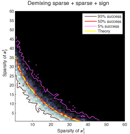
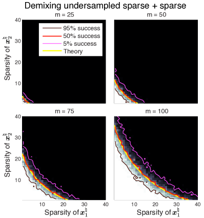
Figure 2: Demixing experiments from Section 4. The colormaps display the empirical probability of successful demixing, from complete success (white) to total failure (black). The transition region (gray) contains a mixture of successes and failures. Three contour lines indicate $95\%$ (brown), $50\%$ (red), and $5\%$ (pink) empirical success lines. The yellow curve indicates where an approximation to the total statistical dimension $\Delta$ equals to the number of measurements $m$. [Left] Demixing two sparse vectors from a sign vector in dimension $d=200$ with complete measurements. [Right] Demixing two sparse vectors in dimension $d=200$ from $m=25,50,75,100$ measurements.

Sparse, sparse, and sign

In our first experiment, we fix the ambient dimension $d=200$ and generate a mixed observation of the form

$$\bm{z}_{0}=\bm{U}_{1}\bm{x}_{1}^{\smash{\natural}}+\bm{U}_{2}\bm{x}_{2}^{\smash{\natural}}+\bm{U}_{3}\bm{x}_{3}^{\smash{\natural}}\in\mathbb{R},$$

where $\bm{x}_{1}^{\smash{\natural}}$ and $\bm{x}_{2}^{\smash{\natural}}$ are sparse vectors, $\bm{x}_{3}^{\smash{\natural}}\in\{\pm 1\}^{d}$ is a sign vector, and the tuple $(\bm{U}_{i})_{i=1}^{3}$ consists of i.i.d. random rotations. In order to demix this observation, we solve the constrained demixing program

$$\operatorname*{minimize}_{\bm{x}_{i}\in\mathbb{R}} \mathopen{}\mathclose{{}\left\|{\bm{U}_{1}\bm{x}_{1}+\bm{U}_{2}\bm{x}_{2}+\bm{U}_{3}\bm{x}_{3}-\bm{z}_{0}}}\right\|^{2}$$ (4.1)

   subject to $$\mathopen{}\mathclose{{}\left\|{\bm{x}_{1}}}\right\|_{{\ell_{1}}\!}\leq\mathopen{}\mathclose{{}\left\|{\bm{x}_{1}^{\smash{\natural}}}}\right\|_{{\ell_{1}}\!},\quad\mathopen{}\mathclose{{}\left\|{\bm{x}_{2}}}\right\|_{{\ell_{1}}\!}\leq\mathopen{}\mathclose{{}\left\|{\bm{x}_{2}^{\smash{\natural}}}}\right\|_{{\ell_{1}}\!},\quad\text{and}\quad\mathopen{}\mathclose{{}\left\|{\bm{x}_{3}}}\right\|_{\ell_{\infty}}\leq\mathopen{}\mathclose{{}\left\|{\bm{x}_{3}^{\smash{\natural}}}}\right\|_{\ell_{\infty}},$$

where $\mathopen{}\mathclose{{}\left\|{\bm{x}}}\right\|_{\ell_{\infty}}:=\max_{i=1,\dotsc,d}|x_{i}|$ is the $\ell_{\infty}$ norm that is a convex penalty function associated to the binary sign vectors $\{\pm 1\}^{d}$.

Figure 2 [left] shows the results of this experiment as the sparsity of $\bm{x}_{1}^{\smash{\natural}}$ and $\bm{x}_{2}^{\smash{\natural}}$ vary. The colormap indicates the empirical probability of success over $35$ trials. The yellow curve uses provably accurate formulas from [ALMT13, Sec. 4] to approximate the location where

$$\delta(\mathopen{}\mathclose{{}\left\|{\cdot}}\right\|_{{\ell_{1}}\!},\bm{x}_{1}^{\smash{\natural}})+\delta(\mathopen{}\mathclose{{}\left\|{\cdot}}\right\|_{{\ell_{1}}\!},\bm{x}_{2}^{\smash{\natural}})+\delta(\mathopen{}\mathclose{{}\left\|{\cdot}}\right\|_{\ell_{\infty}},\bm{x}_{3}^{\smash{\natural}})=d.$$

The agreement between the $50\%$ empirical success curve and the theoretical yellow curve is remarkable. See Appendix E for further details.

Undersampled sparse and sparse

In our second experiment, we fix the ambient dimension $d=200$ and consider demixing the observation

$$\bm{z}_{0}=\bm{A}\bigl{(}\bm{U}_{1}\bm{x}_{1}^{\smash{\natural}}+\bm{U}_{2}\bm{x}_{2}^{\smash{\natural}}\bigr{)},$$

where $\bm{A}\in\mathbb{R}^{m\times d}$ has full row rank, the constituents $\bm{x}_{1}^{\smash{\natural}}$ and $\bm{x}_{2}^{\smash{\natural}}$ are sparse, and $\bm{U}_{1}$ and $\bm{U}_{2}$ are drawn from the random orientation model. We demix the observation by solving

$$\operatorname*{minimize}_{\bm{x}_{i}\in\mathbb{R}} \mathopen{}\mathclose{{}\left\|{\bm{A}^{\dagger}\bigl{(}\bm{A}(\bm{U}_{1}\bm{x}_{1}+\bm{U}_{2}\bm{x}_{2})-\bm{z}_{0}\bigr{)}}}\right\|^{2}$$ (4.2)

   subject to $$\mathopen{}\mathclose{{}\left\|{\bm{x}_{1}}}\right\|_{{\ell_{1}}\!}\leq\mathopen{}\mathclose{{}\left\|{\bm{x}_{1}^{\smash{\natural}}}}\right\|_{{\ell_{1}}\!}\quad\text{and}\quad\mathopen{}\mathclose{{}\left\|{\bm{x}_{2}}}\right\|_{{\ell_{1}}\!}\leq\mathopen{}\mathclose{{}\left\|{\bm{x}_{2}^{\smash{\natural}}}}\right\|_{{\ell_{1}}\!}$$

The results of this experiment with $m=25,50,75$ and $100$ appear in Figure 2 [right]. The colormaps indicate the empirical probability of success over $35$ trials as the sparsity of $\bm{x}_{1}^{\smash{\natural}}$ and $\bm{x}_{2}^{\smash{\natural}}$ varies. The yellow curve approximates the location where

$$\delta(\mathopen{}\mathclose{{}\left\|{\cdot}}\right\|_{{\ell_{1}}\!},\bm{x}_{1}^{\smash{\natural}})+\delta(\mathopen{}\mathclose{{}\left\|{\cdot}}\right\|_{{\ell_{1}}\!},\bm{x}_{2}^{\smash{\natural}})=m.$$

Once again, this yellow curve agrees very well with the red $50\%$ empirical success contour.

5 Conclusions and open problems

This work unifies and resolves a number of theoretical questions regarding when it is possible to demix a superposition of incoherent signals. Under our random incoherence model, we find that demixing is possible if and only if the total number of measurements is greater than the total statistical dimension. While this result provides an intuitive and unifying theory for a large class of demixing problems, there are several important open problems that must be addressed before a complete “theory of demixing” emerges.

Lagrange parameters

Most of the prior work on demixing provides guarantees under explicit choices of the Lagrange parameter for (1.2), yet to the best of our knowledge, the only work that demonstrates sharp recovery bounds with specified Lagrange parameters occur for the LASSO problem, where $n=1$ and $f_{1}=\mathopen{}\mathclose{{}\left\|{\cdot}}\right\|_{{\ell_{1}}\!}$ [BM12]. Very recent work of Stojnic [Sto13] achieves comparable guarantees using a different approach.

Explicit choices of Lagrange parameters appear in [FM13]. These choices provide near-optimal empirical performance, but currently there is no proof that their choice of parameters reaches the phase transition that we identify. It would be very interesting to provide provably optimal choices of Lagrange parameters for demixing.

Other random models

Our numerical experience indicates that the incoherence model considered in this work is predictive for highly incoherent situations. However, these results appear overly optimistic in more coherent situations. The difference between these situations appears, for example, in an application to calcium imaging [PP13, Fig. 3]. Extending our results to other incoherence models will clarify where the phase transition in Theorem A predicts empirical performance, and where it does not.

Statistical dimension calculations

For practical applications of this work, we require accurate statistical dimension calculations. A recipe for these computations put forward in [CRPW12] has provable guarantees under some technical conditions (cf. [ALMT13, Sec. 4.4] and [FM13, Prop. 1]), but expressions for the statistical dimension of a number of important convex regularizers remains unknown. New statistical dimension computations immediately extend the reach of the methods used in this paper.

Appendix A Deterministic conditions

This section provides the deterministic demixing claims of Lemma 3.1. The exact recovery conditions for the noiseless setting appear in Section A.1, and the stable recovery guarantees appear in Section A.2.

A.1 Exact recovery

In this section, we show that, in the noiseless setting $\bm{w}=\bm{0}$ , the tuple $(\bm{x}_{i}^{\smash{\natural}})_{i=1}^{n}$ is the unique optimal point of (1.3) if and only if (ERC) holds.

Suppose first that (ERC) holds, and let $(\hat{\bm{x}}_{i})_{i=1}^{n}$ be any optimal point of (1.3). Define the vectors

$$\bm{y}_{i}:=\hat{\bm{x}}_{i}-\bm{x}_{i}^{\smash{\natural}}\quad\text{for}\quad i=1,\dotsc,n-1,n\quad\text{and}\quad\bm{y}_{n+1}:=-\sum\nolimits_{i=1}^{n}\bm{U}_{i}(\hat{\bm{x}}_{i}-\bm{x}_{i}^{\smash{\natural}}).$$ (A.1)

We will show that $\bm{y}_{i}=\bm{0}$ for each $i=1,\dotsc,n,n+1$. The tuple $(\bm{x}_{i}^{\smash{\natural}})_{i=1}^{n}$ is trivially feasible for (1.3), and the objective at this point is given by

$$\mathopen{}\mathclose{{}\left\|{\bm{A}^{\dagger}\mathopen{}\mathclose{{}\left(\bm{A}\sum\nolimits_{i=1}^{n}\bm{U}_{i}\bm{x}_{i}^{\smash{\natural}}-\bm{z}_{0}}\right)}}\right\|=\mathopen{}\mathclose{{}\left\|{\bm{A}^{\dagger}\bm{A}\bm{0}}}\right\|=0,$$ (A.2)

by definition (1.1) of $\bm{z}_{0}$ and the assumption $\bm{w}=\bm{0}$. Since $(\hat{\bm{x}}_{i})_{i=1}^{n}$ is optimal for (3.1) by assumption, its objective value must be less than the value given in (A.2), which implies

$$0\geq\mathopen{}\mathclose{{}\left\|{\bm{A}^{\dagger}\mathopen{}\mathclose{{}\left(\bm{A}\sum\nolimits_{i=1}^{n}\bm{U}_{i}\hat{\bm{x}}_{i}-\bm{z}_{0}}\right)}}\right\|=\mathopen{}\mathclose{{}\left\|{\bm{A}^{\dagger}\bm{A}(-\bm{y}_{n+1})}}\right\|\geq 0$$

where the equality follows by the definition (A.1) of $\bm{y}_{n+1}$. These sandwiched inequalities imply that

$$\bm{y}_{n+1}\in\mathcal{N}(\bm{A})=D_{n+1}.$$ (A.3)

by the definition (3.1) of $D_{n+1}$. Since an optimal point of (1.3) is also feasible for (1.3), we also have $f_{i}(\hat{\bm{x}}_{i})\leq f_{i}(\bm{x}_{i}^{\smash{\natural}})$. The definition (1.5) of the descent cone implies that

$$\bm{y}_{i}=(\hat{\bm{x}}_{i}-\bm{x}_{i}^{\smash{\natural}})\in\mathcal{D}(f_{i},\bm{x}_{i}^{\smash{\natural}})=D_{i}.$$ (A.4)

By expanding the definition of $\bm{y}_{i}$, we find the trivial relation

$$\sum\nolimits_{i=1}^{n+1}\bm{U}_{i}\bm{y}_{i}=\sum\nolimits_{i=1}^{n}\bm{U}_{i}(\hat{\bm{x}}_{i}-\bm{x}_{i}^{\smash{\natural}})-\bm{U}_{n+1}\mathopen{}\mathclose{{}\left(\sum\nolimits_{i=1}^{n}\bm{U}_{i}(\hat{\bm{x}}_{i}-\bm{x}_{i}^{\smash{\natural}})}\right)=\bm{0},$$

where we recall that $\bm{U}_{n+1}=\mathbf{I}$ by definition (3.1). Upon rearrangement, this equation is equivalent to

$$\bm{U}_{i}\bm{y}_{i}=-\sum\nolimits_{j\neq i}\bm{U}_{j}\bm{y}_{j}\quad\text{for each}\quad i=1,\dotsc,n,n+1.$$

Combined with the containments (A.3) and (A.4), the relations above imply

$$\bm{U}_{i}\bm{y}_{i}\in\bm{U}_{i}D_{i}\cap-\mathopen{}\mathclose{{}\left(\sum\nolimits_{j\neq i}\bm{U}_{j}D_{j}}\right)=\{\bm{0}\}\quad\text{for each}\quad i=1,\dotsc,n,n+1.$$

where the trivial intersection follows because the exact recovery condition (ERC) is in force. Since each $\bm{U}_{i}$ is invertible, we must have $\bm{y}_{i}=\bm{x}_{i}^{\smash{\natural}}-\hat{\bm{x}}_{i}=\bm{0}$ for each $i=1,\dotsc,n$. But $(\hat{\bm{x}}_{i})_{i=1}^{n}$ was an arbitrary optimal point of (1.3), so condition (ERC) indeed implies that the tuple $(\bm{x}_{i}^{\smash{\natural}})_{i=1}^{n}$ is the unique optimum of (1.3).

Now suppose that (ERC) does not hold. Then there exists an index $i_{*}\in\{1,\dotsc,n,n+1\}$ and a vector $\bm{y}_{i_{*}}\neq\bm{0}$ such that

$$\bm{U}_{i_{*}}\bm{y}_{i_{*}}\in\bm{U}_{i_{*}}D_{i_{*}}\cap-\mathopen{}\mathclose{{}\left(\sum\nolimits_{j\neq i_{*}}\bm{U}_{j}D_{j}}\right).$$

Equivalently, there are vectors $\bm{y}_{j}\in D_{j}$ such that

$$\bm{U}_{i_{*}}\bm{y}_{i_{*}}=-\sum\nolimits_{j\neq i_{*}}\bm{U}_{j}\bm{y}_{j}.$$ (A.5)

It follows from the definition of the descent cone and a basic convexity argument (cf. [MT12, Prop. 2.4]) that for some sufficiently small $\tau>0$,

$$f_{i}(\tau\bm{y}_{i}+\bm{x}_{i}^{\smash{\natural}})\leq f_{i}(\bm{x}_{i}^{\smash{\natural}})\quad\text{for all}\quad i=1,\dotsc,n-1,n.$$ (A.6)

Define $\hat{\bm{x}}_{i}:=\tau\bm{y}_{i}+\bm{x}_{i}^{\smash{\natural}}$. The definition $\bm{z}_{0}=\bm{A}\mathopen{}\mathclose{{}\left(\sum_{i=1}^{n}\bm{U}_{i}\bm{x}_{i}^{\smash{\natural}}}\right)$ and (A.5) implies

$$\mathopen{}\mathclose{{}\left\|{\bm{A}^{\dagger}\mathopen{}\mathclose{{}\left(\bm{A}\sum\nolimits_{i=1}^{n}\bm{U}_{i}\hat{\bm{x}}_{i}-\bm{z}_{0}}\right)}}\right\|=\mathopen{}\mathclose{{}\left\|{\bm{A}^{\dagger}\bm{A}(-\tau\bm{U}_{n+1}\bm{y}_{n+1})}}\right\|=0.$$ (A.7)

The final equality follows because $\bm{U}_{n+1}\bm{y}_{n+1}\in\mathcal{N}(\bm{A})$ by definition (3.1).

To summarize, Equation (A.6) shows that the tuple $(\hat{\bm{x}}_{i})_{i=1}^{n}$ is feasible for the constrained demixing program (1.3), while Equation (A.7) indicates that the objective value at $(\hat{\bm{x}}_{i})_{i=1}^{n}$ is the minimum possible. Therefore, $(\hat{\bm{x}}_{i})_{i=1}^{n}$ is an optimal point of (1.3). Since $\bm{y}_{i_{*}}\neq\bm{0}$ and $\tau>0$, we see that $(\hat{\bm{x}}_{i})_{i=1}^{n}\neq(\bm{x}_{i}^{\smash{\natural}})_{i=1}^{n}$. We conclude that $(\bm{x}_{i}^{\smash{\natural}})_{i=1}^{n}$ is not the unique optimal point of (1.3) when (ERC) fails to hold, which completes the exact recovery portion of Lemma 3.1.

A.2 Stable recovery

The stable recovery claims of Lemma 3.1 immediately follow from the next result.

Lemma A.1 (Stability of constrained demixing).

With the notation from definition (3.1), suppose that there exists an $\varepsilon\in(0,1)$ such that

$$\mathopen{}\mathclose{{}\left\llangle-\bm{U}_{i}D_{i},\sum\nolimits_{j\neq i}\bm{U}_{j}D_{j}}\right\rrangle\leq 1-\varepsilon\quad\text{for all}\quad i=1,\dotsc,n,n+1.$$ (A.8)

Then the error bound

$$\mathopen{}\mathclose{{}\left\|{\hat{\bm{x}}_{i}-\bm{x}_{i}^{\smash{\natural}}}}\right\|^{2}\leq\frac{1}{\varepsilon}\mathopen{}\mathclose{{}\left\|{\bm{w}}}\right\|^{2}\quad\text{for all}\quad i=1,\dotsc,n-1,n$$ (A.9)

holds for any optimal point $(\hat{\bm{x}}_{i})_{i=1}^{n}$ of (1.3).

Proof of Lemma 3.1 from Lemma A.1.

Whenever the stable recovery condition (SRC) holds, there is an $\varepsilon>0$ such that the condition (A.8) of Lemma A.1 holds. But (A.9) is equivalent to the definition (1.4) of stable recovery with constant $c=\varepsilon^{-1/2}$. ∎

The proof of Lemma A.1 rests on the following elementary observation.

Proposition A.2.

Suppose $\langle\bm{x},\bm{y}\rangle\geq-(1-\varepsilon)\mathopen{}\mathclose{{}\left\|{\bm{x}}}\right\|\mathopen{}\mathclose{{}\left\|{\bm{y}}}\right\|$ for some $\varepsilon\in(0,1]$. Then

$$\mathopen{}\mathclose{{}\left\|{\bm{x}}}\right\|^{2}+\mathopen{}\mathclose{{}\left\|{\bm{y}}}\right\|^{2}\leq\frac{1}{\varepsilon}\mathopen{}\mathclose{{}\left\|{\bm{x}+\bm{y}}}\right\|^{2}.$$

Proof.

We have the following string of inequalities:

$$\varepsilon\mathopen{}\mathclose{{}\left(\mathopen{}\mathclose{{}\left\|{\bm{x}}}\right\|^{2}+\mathopen{}\mathclose{{}\left\|{\bm{y}}}\right\|^{2}}\right) \leq\varepsilon\mathopen{}\mathclose{{}\left(\mathopen{}\mathclose{{}\left\|{\bm{x}}}\right\|^{2}+\mathopen{}\mathclose{{}\left\|{\bm{y}}}\right\|^{2}}\right)+(1-\varepsilon)\mathopen{}\mathclose{{}\left(\mathopen{}\mathclose{{}\left\|{\bm{x}}}\right\|-\mathopen{}\mathclose{{}\left\|{\bm{y}}}\right\|}\right)^{2}$$

$$=\mathopen{}\mathclose{{}\left\|{\bm{x}}}\right\|^{2}+\mathopen{}\mathclose{{}\left\|{\bm{y}}}\right\|^{2}-2(1-\varepsilon)\mathopen{}\mathclose{{}\left\|{\bm{x}}}\right\|\mathopen{}\mathclose{{}\left\|{\bm{y}}}\right\|$$

$$\leq\mathopen{}\mathclose{{}\left\|{\bm{x}}}\right\|^{2}+\mathopen{}\mathclose{{}\left\|{\bm{y}}}\right\|^{2}+2\langle\bm{x},\bm{y}\rangle$$

The first line follows because squares are nonnegative and $\varepsilon\leq 1$, the second line is algebra, and the final expression relies on our assumption on $\langle\bm{x},\bm{y}\rangle$. The last expression is $\mathopen{}\mathclose{{}\left\|{\bm{x}+\bm{y}}}\right\|^{2}$. ∎

Proof of Lemma A.1.

Define the vectors $\tilde{\bm{y}}_{i}:=(\hat{\bm{x}}_{i}-\bm{x}_{i}^{\smash{\natural}})$ for $i=1,\dotsc,n-1,n$, and

$$\tilde{\bm{y}}_{n+1}:=(\bm{A}^{\dagger}\bm{A}-\mathbf{I})\mathopen{}\mathclose{{}\left(\sum\nolimits_{i=1}^{n}\bm{U}_{i}(\hat{\bm{x}}_{i}-\bm{x}_{i}^{\smash{\natural}})}\right).$$ (A.10)

Since $f_{i}(\hat{\bm{x}}_{i})\leq f_{i}(\bm{x}_{i}^{\smash{\natural}})$ for all $i=1,\dotsc,n$, we have $\tilde{\bm{y}}_{i}\in\bm{\mathcal{D}}(f_{i},\bm{x}_{i}^{\smash{\natural}})$. Moreover, the operator $(\mathbf{I}-\bm{A}^{\dagger}\bm{A})$ is the projection onto the nullspace of $\bm{A}$, so that $\tilde{\bm{y}}_{n+1}\in\mathcal{N}(\bm{A})$. Applying definition (3.1) of the cones $D_{i}$, we see

$$\tilde{\bm{y}}_{i}\in D_{i}\quad\text{for every}\quad i=1,\dotsc,n,n+1.$$

By assumption, $\llangle-\bm{U}_{i}D_{i},\sum\nolimits_{j\neq i}\bm{U}_{j}D_{j}\rrangle\leq 1-\varepsilon$ for each $i=1,\dotsc,n,n+1$, so that

$$\mathopen{}\mathclose{{}\left\langle-\bm{U}_{i}\tilde{\bm{y}}_{i},\sum\nolimits_{j\neq i}\bm{U}_{j}\tilde{\bm{y}}_{i}}\right\rangle\geq-(1-\varepsilon)\mathopen{}\mathclose{{}\left\|{\bm{U}_{i}\tilde{\bm{y}}_{i}}}\right\|\mathopen{}\mathclose{{}\left\|{\sum\nolimits_{j\neq i}\bm{U}_{j}\tilde{\bm{y}}_{j}}}\right\|$$

by definition (1.14) of the angle between cones. Proposition A.2 provides the inequality

$$\mathopen{}\mathclose{{}\left\|{\tilde{\bm{y}}_{i}}}\right\|^{2}\leq\mathopen{}\mathclose{{}\left\|{\bm{U}_{i}\tilde{\bm{y}}_{i}}}\right\|^{2}+\mathopen{}\mathclose{{}\left\|{\sum\nolimits_{j\neq i}\bm{U}_{j}\tilde{\bm{y}}_{j}}}\right\|^{2}\leq\frac{1}{\varepsilon}\mathopen{}\mathclose{{}\left\|{\sum\nolimits_{j=1}^{n+1}\bm{U}_{j}\tilde{\bm{y}}_{j}}}\right\|^{2},$$ (A.11)

where we use the fact that $\mathopen{}\mathclose{{}\left\|{\tilde{\bm{y}}_{i}}}\right\|=\mathopen{}\mathclose{{}\left\|{\bm{U}_{i}\tilde{\bm{y}}_{i}}}\right\|$ because $\bm{U}_{i}$ is orthogonal. Expanding the definitions of $\tilde{\bm{y}}_{i}$ and $\bm{z}_{0}$, we calculate

$$\mathopen{}\mathclose{{}\left\|{\sum\nolimits_{i=1}^{n+1}\bm{U}_{i}\tilde{\bm{y}}_{i}}}\right\|^{2} =\mathopen{}\mathclose{{}\left\|{\bm{A}^{\dagger}\mathopen{}\mathclose{{}\left(\bm{A}\sum\nolimits_{i=1}^{n}\hat{\bm{x}}_{i}-\bm{z}_{0}}\right)+(\mathbf{I}-\bm{A}^{\dagger}\bm{A})\bm{w}}}\right\|^{2}$$

$$=\mathopen{}\mathclose{{}\left\|{\bm{A}^{\dagger}\mathopen{}\mathclose{{}\left(\bm{A}\sum\nolimits_{i=1}^{n}\hat{\bm{x}}_{i}-\bm{z}_{0}}\right)}}\right\|^{2}+\mathopen{}\mathclose{{}\left\|{(\mathbf{I}-\bm{A}^{\dagger}\bm{A})\bm{w}}}\right\|^{2}$$

$$\leq\mathopen{}\mathclose{{}\left\|{\bm{A}^{\dagger}\mathopen{}\mathclose{{}\left(\bm{A}\sum\nolimits_{i=1}^{n}\bm{x}_{i}^{\smash{\natural}}-\bm{z}_{0}}\right)}}\right\|^{2}+\mathopen{}\mathclose{{}\left\|{(\mathbf{I}-\bm{A}^{\dagger}\bm{A})\bm{w}}}\right\|^{2}$$

$$=\mathopen{}\mathclose{{}\left\|{\bm{A}^{\dagger}\bm{A}\bm{w}}}\right\|^{2}+\mathopen{}\mathclose{{}\left\|{(\mathbf{I}-\bm{A}^{\dagger}\bm{A})\bm{w}}}\right\|^{2}.$$

The second equality holds because $(\mathbf{I}-\bm{A}^{\dagger}\bm{A})\bm{A}^{\dagger}=\bm{0}$. For the inequality, note that $(\hat{\bm{x}}_{i})_{i=1}^{n}$ minimizes (1.3) and the tuple $(\bm{x}_{i}^{\smash{\natural}})_{i=1}^{n}$ is feasible for (1.3). The final equality is the definition (1.1) of $\bm{z}_{0}$. Combining the bound above with (A.11), we see

$$\mathopen{}\mathclose{{}\left\|{\hat{\bm{x}}_{i}-\bm{x}_{i}^{\smash{\natural}}}}\right\|^{2}=\mathopen{}\mathclose{{}\left\|{\hat{\bm{y}}_{i}}}\right\|^{2}\leq\frac{1}{\varepsilon}\mathopen{}\mathclose{{}\left(\mathopen{}\mathclose{{}\left\|{\bm{A}^{\dagger}\bm{A}\bm{w}}}\right\|^{2}+\mathopen{}\mathclose{{}\left\|{(\mathbf{I}-\bm{A}^{\dagger}\bm{A})\bm{w}}}\right\|^{2}}\right)=\frac{1}{\varepsilon}\mathopen{}\mathclose{{}\left\|{\bm{w}}}\right\|^{2},$$

where the final relation follows by orthogonality. ∎

Appendix B Simplifying results

This section presents the proofs of the lemmas appearing in Section 3.2.

B.1 Randomizing the nullspace

Lemma 3.2 is an easy consequence of a basic fact about invariant measures.

Fact B.1.

Let $(\bm{Q}_{1},\dotsc,\bm{Q}_{n-1},\bm{Q}_{n})$ be i.i.d. random rotations in $\mathsf{O}_{d}$. Suppose that $f\colon(\mathsf{O}_{d})^{n}\to\mathbb{R}$ is a measurable function that satisfies

$$\operatorname{\mathbb{E}}\Bigl{[}\operatorname{\mathbb{E}}\mathopen{}\mathclose{{}\left[\mathopen{}\mathclose{{}\left|{f(\bm{Q}_{1},\dotsc,\bm{Q}_{n-1},\bm{Q}_{n})}}\right|\;\big{|}\;\bm{Q}_{1}}\right]\Bigr{]}<\infty,$$ (B.1)

where the outer expectation is over $\bm{Q}_{1}$, and the inner expectation is over $\bm{Q}_{i}$ for $i\geq 2$. In particular, condition (B.1) holds when $\mathopen{}\mathclose{{}\left|{f}}\right|$ is bounded. Then

$$\operatorname{\mathbb{E}}[f(\bm{Q}_{1},\bm{Q}_{2},\dotsc,\bm{Q}_{n-1},\bm{Q}_{n})]=\operatorname{\mathbb{E}}[f(\bm{Q}_{1},\bm{Q}_{1}\bm{Q}_{2},\dotsc,\bm{Q}_{1}\bm{Q}_{n-1},\bm{Q}_{1}\bm{Q}_{n})].$$ (B.2)

The elementary proof is a simple application of Fubini’s theorem and the definition of an invariant measure. See [McC13, Fact 3.1] for a detailed proof.

Proof of Lemma 3.2.

Let $\mathbf{1}_{E}\colon(\mathsf{O}_{d})^{n+1}\to\mathbb{R}$ be the indicator function on the event

$$E:=\mathopen{}\mathclose{{}\left\{(\bm{U}_{i})_{i=1}^{n+1}\mathrel{\mathop{:}}-\bm{U}_{i}D_{i}\cap\sum\nolimits_{j\neq i}\bm{U}_{j}D_{j}=\{\bm{0}\}\text{ for each }i=1,\dotsc,n,n+1}\right\},$$

where we recall that the indicator function $\mathbf{1}_{S}$ on a set $S$ is given by

$$\mathbf{1}_{S}(x):=\begin{cases}1,&x\in S,\\ 0,&\text{otherwise}.\end{cases}$$

Let $\tilde{\bm{U}}\in\mathsf{O}_{d}$ be a Haar distributed rotation independent of $(\bm{U}_{i})_{i=1}^{n}$. Since $\tilde{\bm{U}}\{\bm{0}\}=\{\bm{0}\}$ for every rotation, we have the equality

$$\mathbf{1}_{E}(\bm{U}_{1},\dotsc,\bm{U}_{n},\bm{U}_{n+1})=\mathbf{1}_{E}(\tilde{\bm{U}}\bm{U}_{1},\dotsc,\tilde{\bm{U}}\bm{U}_{n},\tilde{\bm{U}}),$$

where we used the fact that $\bm{U}_{n+1}=\mathbf{I}$. Taking expectations, we find

$$\operatorname{\mathbb{E}}[\mathbf{1}_{E}(\bm{U}_{1},\dotsc,\bm{U}_{n},\bm{U}_{n+1})]=\operatorname{\mathbb{E}}[\mathbf{1}_{E}(\tilde{\bm{U}}\bm{U}_{1},\dotsc,\tilde{\bm{U}}\bm{U}_{n},\tilde{\bm{U}})]=\operatorname{\mathbb{E}}[\mathbf{1}_{E}(\bm{Q}_{1},\dotsc,\bm{Q}_{n},\bm{Q}_{n+1})],$$

where we arrive at the last line using (B.2). The first claim (3.2) follows because the average value of the indicator function on an event is equal to the probability of that event. The second claim (3.3) follows in a completely analogous manner, so we omit the details. ∎

B.2 Equivalence between stability and exact recovery

The results below are corollaries of an intuitive fact regarding the configuration of random cones. We first need a definition.

Definition B.2.

Two cones $C,D\in\mathcal{C}_{d}$ are said to touch if they share a ray but are weakly separable by a hyperplane.

When the cones are randomly oriented, touching is almost impossible.

Fact B.3 ([SW08, pp. 258–260]).

Let $C,D\in\mathcal{C}_{d}$ be closed, convex cones such that both $C,D\neq\{\bm{0}\}$. Then

$$\mathbb{P}\{\bm{Q}C\text{ touches }D\}=0,$$

where $\bm{Q}$ is a random rotation in $\mathsf{O}_{d}$.

We will also make use of the separating hyperplane theorem for convex cones due, in a much more general form, to Klee [Kle55, Thm. 2.5].

Fact B.4 (Separating hyperplane theorem for convex cones).

Suppose $C,C^{\prime}$ are two convex cones in $\mathbb{R}$. If $C\cap C^{\prime}=\{\bm{0}\}$, then there exists a nonzero $\bm{z}\in\mathbb{R}$ such that $\bm{z}\in C^{\circ}$ and $-\bm{z}\in(C^{\prime})^{\circ}$.

Proof of Lemma 3.3.

The lemma claims that the events

$$\mathopen{}\mathclose{{}\left\{(\bm{Q}_{i})_{i=1}^{n+1}\mathrel{\mathop{:}}-\bm{Q}_{i}D_{i}\cap\sum\nolimits_{j\neq i}\bm{Q}_{j}D_{j}=\{\bm{0}\}\text{ for each }i=1,\dotsc,n,n+1}\right\}\quad\text{and}\quad$$ (B.3)

$$\mathopen{}\mathclose{{}\left\{(\bm{Q}_{i})_{i=1}^{n+1}\mathrel{\mathop{:}}\mathopen{}\mathclose{{}\left\llangle-\bm{Q}_{i}D_{i},\sum\nolimits_{j\neq i}\bm{Q}_{j}D_{j}}\right\rrangle<1\text{ for each }i=1,\dotsc,n,n+1}\right\}$$ (B.4)

have equal probability when the matrices $\bm{Q}_{i}$ are drawn i.i.d. from the Haar measure on the orthogonal group $\mathsf{O}_{d}$. The event appearing in (B.3) is implied by the event appearing in (B.4), so the probability (B.3) is larger than the probability (B.4). We now show the reverse inequality.

Fix any tuple $(\bm{Q}_{i})_{i=1}^{n+1}$ such that the event (B.3) holds, but that the event (B.4) does not hold. We claim that such a tuple must bring two cones, out of a finite set, into touching position (Definition B.2). The set of all such tuples must have probability zero by Fact B.3 and the countable subadditivity of probability measures. We conclude that the probability of (B.3) is not larger than the probability of (B.4).

We now establish the touching claim. When the event in (3.3) does not hold, there is an index $i$ such that $\bigl{\llangle}-\bm{Q}_{i}D_{i},\sum\nolimits_{j\neq i}\bm{Q}_{j}D_{j}\bigr{\rrangle}=1$. By definition of the angle between cones, we have

$$-\overline{\bm{Q}_{i}D_{i}}\cap\overline{\sum\nolimits_{j\neq i}\bm{Q}_{j}D_{j}}\neq\{\bm{0}\}.$$ (B.5)

But because the event in (B.3) also holds, we have

$$-\bm{Q}_{i}D_{i}\cap\sum\nolimits_{j\neq i}\bm{Q}_{j}D_{j}=\{\bm{0}\}.$$

Hence the separating hyperplane theorem (Fact B.4) shows that $-\bm{Q}_{i}D_{i}$ and $\sum\nolimits_{j\neq i}\bm{Q}_{j}D_{j}$ are weakly separable. By Definition B.2, we see that the cones $-\overline{\bm{Q}_{i}D_{i}}$ and $\overline{\sum\nolimits_{j\neq i}\bm{Q}_{j}D_{j}}$ touch, as claimed. ∎

B.3 Polarizing exact recovery

We bootstrap the proof of Lemma 3.4 from the analogous result for two cones.

Proposition B.5.

Let $C,D\subset\mathbb{R}$ be convex cones that contain zero. If both $C,D\neq\{\bm{0}\}$, then the sets

$$\Bigl{\{}\bm{Q}\in\mathsf{O}_{d}\mathrel{\mathop{:}}-C\cap\bm{Q}D=\{\bm{0}\}\Bigr{\}}\quad\text{and}\quad\Bigl{\{}\bm{Q}\in\mathsf{O}_{d}\mathrel{\mathop{:}}C^{\circ}\cap\bm{Q}D^{\circ}\neq\{\bm{0}\}\Bigr{\}}$$

coincide except on a set of Haar measure zero on $\mathsf{O}_{d}$.

Proof.

Suppose that both $C,D$ are convex cones such that $C,D\neq\{\bm{0}\}$. Whenever $\bm{Q}\in\mathsf{O}_{d}$ is such that $-C\cap\bm{Q}D=\{\bm{0}\}$, the separating hyperplane theorem for convex cones (Fact B.4) ensures there exists a nonzero vector $\bm{w}\in\mathbb{R}$ such that

$$\langle\bm{w},\bm{x}\rangle\leq 0\;\text{for all }\bm{x}\in C\quad\text{and}\quad\langle\bm{w},\bm{Q}\bm{y}\rangle\leq 0\;\text{for all }\bm{y}\in D.$$ (B.6)

This is equivalent to the statement $\bm{w}\in C^{\circ}\cap\bm{Q}D^{\circ}$ by definition (1.13) of polar cones. Since $\bm{w}$ is nonzero, we have the inclusion

$$\Bigl{\{}\bm{Q}\mathrel{\mathop{:}}-C\cap\bm{Q}D=\{\bm{0}\}\Bigr{\}}\subset\Bigl{\{}\bm{Q}\mathrel{\mathop{:}}C^{\circ}\cap\bm{Q}D^{\circ}\neq\{\bm{0}\}\Bigr{\}}.$$

For the other direction, suppose that $C^{\circ}\cap\bm{Q}D^{\circ}\neq\{\bm{0}\}$ for some rotation $\bm{Q}\in\mathsf{O}_{d}$. By definition of polar cones, this implies the existence of a vector $\bm{w}\neq\bm{0}$ satisfying (B.6)—in other words, some nonzero vector weakly separates the cone $-C$ from $\bm{Q}D$. We therefore find two alternatives: either $-C\cap\bm{Q}D=\{\bm{0}\}$, or the closures $-\overline{C}$ and $\bm{Q}\overline{D}$ touch (cf. Definition B.2). In event notation, we have the inclusion

$$\Bigl{\{}\bm{Q}\mathrel{\mathop{:}}C^{\circ}\cap\bm{Q}D^{\circ}\neq\{\bm{0}\}\Bigr{\}}\subset\Bigl{\{}\bm{Q}\mathrel{\mathop{:}}-C\cap\bm{Q}D=\{\bm{0}\}\Bigr{\}}\cup\Bigl{\{}\bm{Q}\mathrel{\mathop{:}}-\overline{C}\text{ touches }\bm{Q}\overline{D}\Bigr{\}}.$$

But randomly oriented, nontrivial, closed cones touch with probability zero by Fact B.3, so the third set above has measure zero. The conclusion follows by combining the two displayed inclusions. ∎

Proof of Lemma 3.4.

For each $i=1,\dotsc,n,n+1$, define $E_{i}\subset(\mathsf{O}_{d})^{n+1}$ and $E_{\circ}\subset(\mathsf{O}_{d})^{n+1}$ by

$$E_{i}:=\mathopen{}\mathclose{{}\left\{-\bm{Q}_{i}D_{i}\cap\sum\nolimits_{j\neq i}\bm{Q}_{j}D_{j}=\{\bm{0}\}}\right\}\quad\text{and}\quad E_{\circ}:=\bigl{\{}\bm{Q}_{1}D_{1}^{\circ}\cap\dotsb\cap\bm{Q}_{n}D_{n}^{\circ}\cap\bm{Q}_{n+1}D_{n+1}^{\circ}\neq\{\bm{0}\}\bigr{\}}.$$

With this notation, the statement of Lemma 3.4 is equivalent to the claim

$$\mathbb{P}\mathopen{}\mathclose{{}\left(\bigcap\nolimits_{i=1}^{n+1}E_{i}}\right)=\mathbb{P}(E_{\circ}).$$ (B.7)

Let $J\subset\{1,\dotsc,n,n+1\}$ be the set of indices $j$ such that $D_{j}\neq\{\bm{0}\}$. For any $k\notin J$, the event $E_{k}$ always occurs:

$$\mathbb{P}(E_{k})=\mathbb{P}\mathopen{}\mathclose{{}\left\{-\{\bm{0}\}\cap\sum\nolimits_{i\neq k}\bm{Q}_{k}D_{k}=\{\bm{0}\}}\right\}=1$$

because $D_{k}=\{\bm{0}\}$ for $k\notin J$ by definition. Therefore,

$$\mathbb{P}\mathopen{}\mathclose{{}\left(\bigcap\nolimits_{j=1}^{n+1}E_{j}}\right)=\mathbb{P}\mathopen{}\mathclose{{}\left(\bigcap\nolimits_{j\in J}E_{j}}\right).$$ (B.8)

Note that this relation requires that $J$ is not empty, which holds true because we assume that $D_{j}\neq\{\bm{0}\}$ for at least two cones. For each $j\in J$, both relations

$$D_{j}\neq\{\bm{0}\}\quad\text{and}\quad\sum\nolimits_{k\neq j}\bm{Q}_{k}D_{k}\neq\{\bm{0}\}$$

hold. Indeed, the left-hand relation is the definition of $J$, while the right-hand relation follows because at least one of the remaining cones is nontrivial by assumption. From Proposition B.5, for $j\in J$, the event $E_{j}$ is equal to $E_{\circ}$ except on a set of measure zero. Since finite unions and intersections of null sets are null, the intersection $\bigcap_{j\in J}E_{j}$ is equal to $E_{\circ}$ except on a set of measure zero. In particular,

$$\mathbb{P}\mathopen{}\mathclose{{}\left(\bigcap\nolimits_{j\in J}E_{j}}\right)=\mathbb{P}(E_{\circ}).$$

Combining this equality with (B.8) proves that (B.7) holds, which completes the claim. ∎

Appendix C The approximate kinematic formula

The approximate kinematic formula is the main tool we use to derive the probability bounds in Theorem A. This new formula extends the result [ALMT13, Thm. 7.1] to an arbitrary number of cones, and it incorporates several technical improvements from the recent work [MT13].

At its core, the approximate kinematic formula is based on an exact kinematic formula for convex cones. This kinematic formula is classical [San76], and the form we use here can be found, for example, in [SW08, Sec. 6.5]. Our derivation requires some background in conic integral geometry; we collect the relevant definitions and facts in Section C.1. The proof of the approximate kinematic formula appears in Section C.2.

C.1 Background from conic integral geometry

We start by defining the core parameters associated with convex cones.

Definition C.1 (Intrinsic volumes [McM75]).

Let $C\in\mathcal{C}_{d}$ be a polyhedral cone. For each $i=0,\dotsc,d-1,d$, the $i$th (conic) intrinsic volume $v_{i}(C)$ is equal to the probability that a Gaussian random vector projects into an $i$-dimensional face of $C$, that is

$$v_{i}(C):=\mathbb{P}\Bigl{\{}\bm{\Pi}_{C}(\bm{g})\in\operatorname{relint}(F_{i})\;\mathrel{\mathop{:}}\;F_{i}\text{ is an $i$-dimensional face of }C\Bigr{\}}.$$ (C.1)

This definition extends to all cones in $\mathcal{C}_{d}$ by approximation with polyhedral cones.

The next fact collects some basic facts about the intrinsic volumes.

Fact C.2 (Intrinsic volumes properties).

For any closed, convex cone $C\in\mathcal{C}_{d}$, the following relations hold.

1. Probability. The intrinsic volumes form a probability distribution:

   $$\sum\nolimits_{i=0}^{d}v_{i}(C)=1\quad\text{and}\quad v_{i}(C)\geq 0.$$ (C.2)

2. Polarity. The intrinsic volumes reverse under polarity:

   $$v_{k}(C)=v_{d-k}(C^{\circ})$$ (C.3)

3. Product. For any $C^{\prime}\in\mathcal{C}_{d^{\prime}}$, the intrinsic volumes of the product $C\times C^{\prime}$ satisfy

   $$v_{k}(C\times C^{\prime})=\sum\nolimits_{i+j=k}v_{i}(C)v_{j}(C^{\prime}).$$ (C.4)

4. Subspace. For an $m$-dimensional subspace $L\subset\mathbb{R}$, we have

   $$v_{k}(L)=\begin{cases}1,&k=m,\\ 0,&\text{otherwise}.\end{cases}$$ (C.5)

All of these facts appear in [ALMT13, Sec. 5.1]. For future reference, we note here that (C.4) and (C.5) together imply that for any $C\in\mathcal{C}_{d}$ and $m$-dimensional linear subspace $L$, we have

$$v_{k}(C\times L)=v_{k-m}(C)$$ (C.6)

whenever $k\geq m$.

Sums and partial sums of intrinsic volumes appear frequently in the theory of conic integral geometry, so we make the following definitions to simplify the later development. For any cone $C\in\mathcal{C}_{d}$ and index $k=0,\dotsc,d-1,d$, we define the $k$th tail-functional $t_{k}(C)$ by

$$t_{k}(C) :=v_{k}(C)+v_{k+1}(C)+\dotsb=\sum\nolimits_{j=k}^{d}v_{k}(C)$$ (C.7)

and the $$k$$th half-tail functional

$$h_{k}(C) :=v_{k}(C)+v_{k+2}(C)+\dotsb=\sum_{\begin{subarray}{c}j=k\\ j-k\text{ even}\end{subarray}}^{d}v_{j}(C).$$ (C.8)

The tail functionals satisfy the following properties.

Fact C.3 (Properties of the tail functionals).

Let $C\in\mathcal{C}_{d}$ be a closed, convex cone.

1. Gauss–Bonnet. [SW08, Eq. (6.55)]

   $$2h_{1}(C)=\begin{cases}0,&C\text{ an even-dimensional subspace}\\ 2,&C\text{ an odd-dimensional subspace}\\ 1,&\text{otherwise}\end{cases}$$ (C.9)

2. Interlacing. [ALMT13, Prop. 5.7] If $C$ is not a linear subspace, then

   $$h_{k}(C)\geq\frac{1}{2}t_{k}(C)\geq h_{k+1}(C)\quad\text{for every}\quad k=0,\dotsc,d-1,d.$$ (C.10)

3. Duality. [ALMT13, Eq. (6.9)] We have the duality formula

   $$t_{k}(C)=1-t_{d-k+1}(C^{\circ}).$$ (C.11)

C.1.1 Kinematic formulas

For any two cones $C,C^{\prime}\in\mathcal{C}_{d}$, the classical conic kinematic formula states [SW08, Eq. (6.61)]

$$\operatorname{\mathbb{E}}[v_{k}(C\cap\bm{Q}D)]=v_{d+k}(C\times D)\quad\text{for}\quad k=1,\dotsc,d-1,d,$$ (C.12)

where the expectation is over the random rotation $\bm{Q}$. Note that our indices are shifted compared to the reference, and we have simplified the expression using the product rule (C.4). Using an inductive argument, we can extend this formula to the product of a finite number of cones.

Fact C.4 (Iterated kinematic formula).

Let $C_{1},\dotsc,C_{n-1},C_{n}\in\mathcal{C}_{d}$ be closed, convex cones and suppose that $\bm{Q}_{1},\dotsc,\bm{Q}_{n-1},\bm{Q}_{n}$ are i.i.d. random rotations. Then for all $k=1,\dotsc,d-1,d$, we have

$$\operatorname{\mathbb{E}}[v_{k}(\bm{Q}_{1}C_{1}\cap\dotsb\cap\bm{Q}_{n-1}C_{n-1}\cap\bm{Q}_{n}C_{n})]=v_{(n-1)d+k}(C_{1}\times\dotsb\times C_{n-1}\times C_{n}).$$ (C.13)

The details are straightforward, so we refer to [McC13, Prop. 5.12] for the proof. See [SW08, Thm. 5.13] for the analogous proof in the Euclidean setting. A related fact is the following Crofton formula for the probability that convex cones intersect nontrivially.

Fact C.5 (Iterated Crofton formula).

Let $C_{1},\dotsc,C_{n-1},C_{n}\in\mathcal{C}_{d}$ be closed, convex cones, at least one of which is not a subspace. Suppose $\bm{Q}_{1},\dotsc,\bm{Q}_{n-1},\bm{Q}_{n}\in\mathsf{O}_{d}$ are independent random rotations. Then

$$\mathbb{P}\Bigl{\{}\bm{Q}_{1}C_{1}\cap\dotsb\cap\bm{Q}_{n-1}C_{n-1}\cap\bm{Q}_{n}C_{n}\neq\{\bm{0}\}\Bigr{\}}=2h_{(n-1)d+1}(C_{1}\times\dotsb\times C_{n-1}\times C_{n}).$$ (C.14)

The proof, which appears in [McC13, Cor. 5.13], simply combines the Gauss–Bonnet formula (C.9) with the kinematic formula (C.13). The only obstacle involves verifying that the intersection of cones is almost surely not an odd-dimensional subspace so long as one of the cones in the intersection is not a subspace. This technical point is proved in detail in [McC13, Lem. 5.13].

C.2 Proof of the approximate kinematic formula

The proof of Theorem A begins with a concentration inequality for tail functionals.

Proposition C.6 (Concentration of tail functionals).

Let $C_{1},\dotsc,C_{n-1},C_{n}\in\mathcal{C}_{d}$ and let $\Omega$ and $\theta$ be as in (3.5). Then for any $\lambda>0$ and integer $k\geq\Omega+\lambda$, we have

$$t_{k}(C_{1}\times\dotsb\times C_{n-1}\times C_{n})\leq p_{\theta}(\lambda);$$ (C.15)

Proof.

We follow the argument of [MT13, Cor. 5.2]. For any cone $C\in\mathcal{C}_{d}$, we define the intrinsic volume random variable $V_{C}$ on $\{0,1,\dotsc,d\}$ by its distribution:

$$\mathbb{P}\{V_{C}=i\}=v_{i}(C).$$

The mean value of $V_{C}$ is equal to the statistical dimension, that is, $\operatorname{\mathbb{E}}[V_{C}]=\delta(C)$ [MT13, Sec. 4.2]. The product rule (C.4) for intrinsic volumes implies $V_{C_{1}\times\dotsb\times C_{n-1}\times C_{n}}=\sum\nolimits_{i=1}^{n}V_{C_{i}}$ because the distribution of a sum of independent random variables is equal to the convolution of the distributions. In particular,

$$\operatorname{\mathbb{E}}[V_{C_{1}\times\dotsc\times C_{n-1}\times C_{n}}]=\delta(C_{1}\times\dotsb\times C_{n-1}\times C_{n})=\sum\nolimits_{i=1}^{n}\delta(C_{i})=\Omega.$$

With these facts in hands, we can complete the proof by tracing the argument leading to [MT13, Cor. 5.2]. The exponential moment of $V_{C_{1}\times\dotsb\times C_{n-1}\times C_{n}}$ factors as

$$\operatorname{\mathbb{E}}\mathrm{e}^{\zeta(V_{C_{1}\times\dotsc,\times C_{n}}-\Omega)}=\prod\nolimits_{i=1}^{n}\operatorname{\mathbb{E}}\mathrm{e}^{\zeta(V_{C_{i}}-\delta(C_{i}))}\leq\exp\mathopen{}\mathclose{{}\left(\frac{\zeta^{2}\theta^{2}}{1-2\mathopen{}\mathclose{{}\left|{\zeta}}\right|/3}}\right)\quad\text{for any}\quad\mathopen{}\mathclose{{}\left|{\zeta}}\right|<3/2,$$ (C.16)

where the inequality follows from [MT13, Thm. 4.8] and the bound

$$\frac{\mathrm{e}^{2\zeta}-2\zeta-1}{2}\leq\frac{\zeta^{2}}{1-2|\zeta|/3}\quad\text{for all}\quad\mathopen{}\mathclose{{}\left|{\zeta}}\right|\leq\frac{3}{2}.$$

Combining the moment bound (C.16) with the Laplace transform method under the choice $\zeta=\lambda/(2\theta^{2}+2\lambda/3)$ provides

$$t_{\lceil\Omega+\lambda\rceil}(C_{1}\times\dotsc\times C_{n})=\mathbb{P}\{V_{C_{1}\times\cdots\times C_{n}}\geq\Omega+\lambda\}\leq\exp\mathopen{}\mathclose{{}\left(\frac{-\lambda^{2}/4}{\theta^{2}+\lambda/3}}\right).$$

The first equality above is the definition (C.7) of the tail functional. Inequality (C.15) follows because the integer $k\geq\Omega+\lambda$ and the tail functionals are decreasing in $k$. ∎

Proof of Theorem 3.5.

A simple dimension-counting argument shows that we incur no loss by assuming that at least one of the cones $C_{1},\dotsc,C_{n-1},C_{n}$ is not a subspace. Indeed, recall from linear algebra that two generically oriented subspaces intersect nontrivially with probability zero if the sum of their dimensions is less or equal to the ambient dimension, but they intersect with probability one if the sum of their dimensions is greater than the ambient dimension. When all of the cones are subspaces, the term $\Omega$ is just the sum of the dimensions of the subspaces $C_{i}$. Evidently, when all of the cones are subspaces, the implications (3.6) and (3.7) hold with respective probability bounds zero and one.

Suppose then that at least one of the cones is not a subspace. For $\Omega+m\leq nd-\lambda$, the iterated kinematic formula (C.14) bounds the probability of interest by

$$\mathbb{P}\bigl{\{}\bm{Q}_{1}C_{1}\cap\dotsb\cap\bm{Q}_{n}C_{n}\cap\bm{Q}_{n+1}L\neq\{\bm{0}\}\bigr{\}} =2h_{nd+1}(C_{1}\times\dotsb\times C_{n}\times L)$$ (C.17)

$$\leq t_{nd}(C_{1}\times\dotsb\times C_{n}\times L),$$

where the inequality follows from the interlacing result (C.10). Equation (C.6) and the upper tail bound (C.15) provides

$$t_{nd}(C_{1}\times\dotsb\times C_{n}\times L)=t_{nd-m}(C_{1}\times\dotsb\times C_{n})\leq p_{\sigma}(\lambda).$$

This completes the first claim (3.6).

The second claim follows along similar lines. Suppose that $\Omega+m\geq nd+\lambda$. Combining the iterated kinematic formula (C.17) with the lower interlacing inequality (C.10), we see

$$\mathbb{P}\bigl{\{}\bm{Q}_{1}C_{1}\cap\dotsb\cap\bm{Q}_{n}C_{n}\cap\bm{Q}_{n+1}L\neq\{\bm{0}\}\bigr{\}} \geq t_{nd+1}(C_{1}\times\dotsb\times C_{n}\times L)$$

$$=1-t_{d}(C_{1}^{\circ}\times\dotsb\times C_{n}^{\circ}\times L^{\perp}),$$ (C.18)

where the final relation is (C.11). Using (C.6) to shift the index of the tail functional, we find

$$t_{d}(C_{1}^{\circ}\times\dotsb\times C_{n}^{\circ}\times L^{\perp})=t_{m}(C_{1}^{\circ}\times\dotsb\times C_{n}^{\circ})\leq p_{\sigma}(\lambda).$$ (C.19)

The final inequality follows from the approximate kinematic formula (C.15), which applies because

$$m\geq(nd-\Omega)+\lambda=\sum\nolimits_{i=1}^{n}\delta(C_{i}^{\circ})+\lambda$$

by assumption and the polarity formula (1.15). The final claim (3.7) follows by combining (C.18) and (C.19). ∎

Appendix D Degenerate case of the main theorem

Proof of Theorem A for the degenerate case..

We now consider the degenerate situation where all except possibly one of the cones $(D_{i})_{i=1}^{n}$ is equal to the trivial cone $\{\bm{0}\}$. In this case, the restrictions in Lemma 3.4 preclude using the polar optimality condition (3.4). Instead, we study the success probability (3.2) directly.

By our assumption, there is an index $i_{*}\in\{1,\dotsc,n,n-1\}$ such that

$$D_{i}=\{\bm{0}\}\quad\text{for all}\quad i\in\{1,\dotsc,n,n+1\}\setminus\{i_{*}\}.$$

This implies that

$$\text{either}\quad\bm{Q}_{i}D_{i}=\{\bm{0}\}\quad\text{or}\quad\sum\nolimits_{j\neq i}\bm{Q}_{j}D_{j}=\{\bm{0}\}$$

for every $i=1,\dotsc,n,n+1$. Therefore, the probability (3.2) is equal to one, so that $(\bm{x}_{i}^{\smash{\natural}})_{i=1}^{n}$ is almost surely the unique optimal point of the constrained demixing method (1.3) by Lemmas 3.1 and 3.2. Since (SRC) holds with the same probability that (ERC) holds under the random orientation model (Lemma 3.3), we only need to verify that the left-hand side of the implication (1.11) never holds.

By definition of $\Delta$ and $i_{*}$, we have

$$\Delta+d-m=\sum\nolimits_{i=1}^{n+1}\delta(D_{i})=\delta(D_{i_{*}})\leq d$$ (D.1)

because the statistical dimension is always less than the ambient dimension. Rearranging, we find

$$m\geq\Delta>\Delta-\lambda_{*}$$

because $\lambda_{*}>0$. Hence, the left-hand side of the implication (1.11) never holds. ∎

Appendix E Numerical details

This section provides some specific numerical details of the experiments described in Section 4.

Numerical environment.

All computations are performed using the Matlab computational platform. We generate i.i.d. rotations from the orthogonal group using the method described in [Mez07]. We solve (1.3) numerically using the CVX package [GB08, GB10] for Matlab. All numerical precision settings are set at the default. The empirical level sets appearing in Figure 2 are determined using the contour function.

Computing the statistical dimension.

In order to draw the yellow curves in Figure 2, we make use known statistical dimension computations. The statistical dimension $\delta(\mathopen{}\mathclose{{}\left\|{\cdot}}\right\|_{\ell_{\infty}},\bm{x})=d/2$ whenever $\bm{x}\in\{\pm 1\}^{d}$ because the descent cone $\mathcal{D}(\mathopen{}\mathclose{{}\left\|{\cdot}}\right\|_{\ell_{\infty}},\bm{x}_{3}^{\smash{\natural}})$ is isometric to the positive orthant $\mathbb{R}_{+}=\{\bm{x}\mathrel{\mathop{:}}x_{i}\geq 0\;\forall\;i=1,\dotsc,d-1,d\}$ that has statistical dimension $\delta(\mathbb{R}_{+})=d/2$ [ALMT13, Sec. 4.2].

We estimate the statistical dimension of the descent cone of the $\ell_{1}$ norm at sparse vectors by solving the implicit formulas appearing in [ALMT13, Eqs. (4.12) & (4.13)] using Matlab’s fzero function. These equations define a function $\psi\colon(0,1)\to(0,1)$ that satisfies

$$\psi(k/d)-\frac{2}{\sqrt{kd}}\leq\frac{\delta(\mathopen{}\mathclose{{}\left\|{\cdot}}\right\|_{{\ell_{1}}\!},\bm{x})}{d}\leq\psi(k/d)$$ (E.1)

for every vector $\bm{x}\in\mathbb{R}$ with $k$ nonzero elements. The function $d\cdot\psi$ thus provides and accurate approximation to the statistical dimension $\delta(\mathopen{}\mathclose{{}\left\|{\cdot}}\right\|_{{\ell_{1}}\!},\bm{x})$.

Sparse, sparse, and sign

The experiment seen in Figure 2 [left] was conducted using the following procedure. Fix the ambient dimension $d=200$ and for each sparsity $k_{1},k_{2}\in\{1,\dotsc,59,60\}$, we repeat the following steps $25$ times:

1. Draw $\bm{U}_{1}$, $\bm{U}_{2}$, and $\bm{U}_{3}$ i.i.d. from the orthogonal group $\mathsf{O}_{d}$.

2. For $i=1,2$, generate independent sparse vectors $\bm{x}_{i}$ with $k_{i}$ nonzero elements by selecting the support uniformly at random and setting each nonzero element $\{\pm 1\}$ independently and with equal probability.

3. Draw $\bm{x}_{3}^{\smash{\natural}}$ by choosing each elements from $\{\pm 1\}$ independently and with equal probability.

4. Compute $\bm{z}_{0}=\bm{U}_{1}\bm{x}_{1}^{\smash{\natural}}+\bm{U}_{2}\bm{x}_{2}^{\smash{\natural}}+\bm{U}_{3}\bm{x}_{3}^{\smash{\natural}}$.

5. Solve (4.1) for an optimal point $(\hat{\bm{x}}_{i})_{i=1}^{3}$ using CVX.

6. Declare success if $\mathopen{}\mathclose{{}\left\|{\hat{\bm{x}}_{i}-\bm{x}_{i}^{\smash{\natural}}}}\right\|_{\ell_{\infty}}<10^{-5}$ for each $i=1,2,3$.

Figure 2 [left] shows the results of this experiment. The colormap indicates the empirical probability of success for each value of $k_{1}$ and $k_{2}$. To compare this experiment to the guarantees of Theorem A, we plot the curve (yellow) in $(k_{1},k_{2})$-space such that

$$d\,\psi\mathopen{}\mathclose{{}\left(\tfrac{k_{1}}{d}}\right)+d\,\psi\mathopen{}\mathclose{{}\left(\tfrac{k_{2}}{d}}\right)=\frac{d}{2}$$

where $\psi(k/d)\approx\delta(\mathopen{}\mathclose{{}\left\|{\cdot}}\right\|_{{\ell_{1}}\!},\bm{x})$ at $k$-sparse vectors $\bm{x}$ (cf. (E.1)). Recalling that $\delta(\mathopen{}\mathclose{{}\left\|{\cdot}}\right\|_{\ell_{\infty}},\bm{x}_{3}^{\smash{\natural}})=d/2$, we see that the yellow curve in Figure 2 [left] shows the approximate center of the phase transition between success and failure predicted by Theorem A. It matches the empirical $50\%$ success level set (red) very closely.

Undersampled sparse and sparse

We fix the ambient dimension $d=200$ and for each pair of sparsity levels $k_{1},k_{2}\in\{1,\dotsc,39,40\}$ and measurement number $m\in\{25,50,75,100\}$, we repeat the following procedure $35$ times:

1. Draw the matrix $\bm{A}\in\mathbb{R}^{m\times d}$ with i.i.d. standard Gaussian entries and the rotations $\bm{U}_{1},\bm{U}_{2}\in\mathsf{O}_{d}$ i.i.d. from the orthogonal group $\mathsf{O}_{d}$.

2. Generate independent sparse vectors $\bm{x}_{1}^{\smash{\natural}}$ and $\bm{x}_{2}^{\smash{\natural}}$ with $k_{1}$ and $k_{2}$ nonzero elements using the same method as above.

3. Compute $\bm{z}_{0}=\bm{A}(\bm{U}_{1}\bm{x}_{1}^{\smash{\natural}}+\bm{U}_{2}\bm{x}_{2}^{\smash{\natural}})$.

4. Solve (4.2) for an optimal point $(\hat{\bm{x}}_{i})_{i=1}^{2}$ using CVX.

5. Declare success if $\mathopen{}\mathclose{{}\left\|{\hat{\bm{x}}_{i}-\bm{x}_{i}^{\smash{\natural}}}}\right\|_{\ell_{\infty}}<10^{-5}$ for $i=1,2$.

We present the results of this experiment in Figure 2 [right]. The colormap denotes the empirical probability of success for different values of $k_{1}$ and $k_{2}$, and each subpanel displays the results for a different value of $m$. Each subpanel also displays the curve (yellow) where

$$d\,\psi\mathopen{}\mathclose{{}\left(\tfrac{k_{1}}{d}}\right)+d\,\psi\mathopen{}\mathclose{{}\left(\tfrac{k_{2}}{d}}\right)=m.$$

The bound (E.1) guarantees that this curve is close to the theoretical phase transition predicted by Theorem A. Again, we find very close agreement between the yellow curve and the empirical $50\%$ success level set.

References

- [ALMT13] Dennis Amelunxen, Martin Lotz, Michael B. McCoy, and Joel A. Tropp. Living on the edge: A geometric theory of phase transitions in convex optimization. preprint, March 2013. arXiv:1303.6672.
- [BM12] Mohsen Bayati and Andrea Montanari. The LASSO risk for Gaussian matrices. IEEE Trans. Inform. Theory, 58(4):1997–2017, April 2012.
- [BMS06] Jérôme Bobin, Yassir Moudden, and Jean-Luc Starck. Morphological diversity and source separation. IEEE Trans. Signal Process., 13(7):409–412, 2006.
- [BSF+07] Jérôme Bobin, Jean-Luc Starck, Jalal M Fadili, Yassir Moudden, and David L. Donoho. Morphological component analysis: an adaptive thresholding strategy. IEEE Trans. Image Process., 16(11):2675–2681, November 2007.
- [BSFM07] Jérôme Bobin, Jean-Luc Starck, Jalal Fadili, and Yassir Moudden. Sparsity and morphological diversity in blind source separation. IEEE Trans. Image Process., 16(11):2662–2674, November 2007.
- [CJSC11a] Yudong Chen, Ali Jalali, Sujay Sanghavi, and Constantine Caramanis. Clustering partially observed graphs via convex optimization. In International Symposium on Information Theory (ISIT), 2011.
- [CJSC11b] Yudong Chen, Ali Jalali, Sujay Sanghavi, and Constantine Caramanis. Low-rank matrix recovery from errors and erasures. In International Symposium on Information Theory (ISIT), pages 2313–2317, August 2011.
- [CJSC13] Yudong Chen, Ali Jalali, Sujay Sanghavi, and Constantine Caramanis. Low-rank matrix recovery from errors and erasures. IEEE Trans. Inform. Theory., 59(7):4324–4337, 2013.
- [CLMW11] Emmanuel J. Candès, Xiadong Li, Yi Ma, and John Wright. Robust principal component analysis? J. Assoc. Comput. Mach., 58(3):1–37, May 2011.
- [CPW10] Venkat Chandrasekaran, Pablo A. Parrilo, and Alan S. Willsky. Latent variable graphical model selection via convex optimization. In 48th Annual Allerton Conference on Communication, Control, and Computing (Allerton), pages 1610–1613, October 2010.
- [CRPW12] Venkat Chandrasekaran, Benjamin Recht, Pablo A. Parrilo, and Alan S. Willsky. The convex geometry of linear inverse problems. Found. Comput. Math., 12(6):805–849, 2012.
- [CSPW09] Venkat Chandrasekaran, Sujay Sanghavi, Pablo A. Parrilo, and Alan S. Willsky. Sparse and low-rank matrix decompositions. In SYSID 2009, Saint-Malo, France, July 2009.
- [CSPW11] Venkat Chandrasekaran, Sujay Sanghavi, Pablo A. Parrilo, and Alan S. Willsky. Rank-sparsity incoherence for matrix decomposition. SIAM J. Optim, 21(2):572–596, 2011.
- [CT05] Emmanuel J. Candès and Terence Tao. Decoding by linear programming. IEEE Trans. Inform. Theory, 51(12):4203–4215, 2005.
- [DH01] David L. Donoho and Xiaoming Huo. Uncertainty principles and ideal atomic decomposition. IEEE Trans. Inform. Theory, 47(7):2845–2862, August 2001.
- [Don06] David L. Donoho. Compressed sensing. IEEE Trans. Inform. Theory, 52(4):1289–1306, 2006.
- [DS89] David L. Donoho and Philip B. Stark. Uncertainty principles and signal recovery. SIAM J. Appl. Math., 49(3):906–931, June 1989.
- [DT96] Ronald A. DeVore and Vladimir N. Temlyakov. Some remarks on greedy algorithms. Adv. Comput. Math., 5(2-3):173–187, 1996.
- [DT10] David L. Donoho and Jared Tanner. Counting the faces of randomly-projected hypercubes and orthants, with applications. Discrete Comput. Geom., 43(3):522–541, 2010.
- [ESQD05a] Michael Elad, Jean-Luc Starck, Philippe Querre, and David L. Donoho. Simultaneous cartoon and texture image inpainting using morphological component analysis (MCA). Appl. Comput. Harmon. Anal., 19(3):340–358, November 2005.
- [ESQD05b] Michael Elad, Jean-Luc Starck, Philippe Querre, and David L. Donoho. Simultaneous cartoon and texture image inpainting using morphological component analysis (MCA). Appl. Comput. Harmon. Anal., 19(3):340–358, November 2005.
- [Faz02] Maryam Fazel. Matrix rank minimization with applications. Dissertation, Stanford University, Stanford, CA, 2002.
- [FM13] Rina Foygel and Lester Mackey. Corrupted sensing: Novel guarantees for separating structured signals. preprint, 2013. arXiv:1305.2524.
- [Fre06] David H. Fremlin. Measure Theory, volume 4. Torres Fremlin, Colchester, 2006. Topological measure spaces. Part I, II, Corrected second printing of the 2003 original.
- [GB08] Michael Grant and Stephen Boyd. Graph implementations for nonsmooth convex programs. In V. Blondel, S. Boyd, and H. Kimura, editors, Recent Advances in Learning and Control, Lecture Notes in Control and Information Sciences, pages 95–110. Springer-Verlag Limited, London, 2008. http://stanford.edu/~boyd/graph_dcp.html.
- [GB10] Michael Grant and Stephen Boyd. CVX: Matlab software for disciplined convex programming, version 1.21. Online. Available http://cvxr.com/cvx, October 2010.
- [Gla95] Stefan Glasauer. Integralgeometrie konvexer Körper im sphärischen Raumrischen Raum. Dissertation, University of Freiburg, 1995.
- [JRSR10] Ali Jalali, Pradeep Ravikumar, Sujay Sanghavi, and Chao Ruan. A dirty model for multi-task learning. In J. Lafferty, C.K.I. Williams, J. Shawe-Taylor, R.S. Zemel, and A. Culotta, editors, Advances in Neural Information Processing Systems 23, pages 964–972. NIPS, 2010.
- [JRSR11] Ali Jalali, Pradeep Ravikumar, Sujay Sanghavi, and Chao Ruan. A dirty model for multiple sparse regression. preprint, 2011. arXiv:1106.5826.
- [Kle55] Victor L. Klee, Jr. Separation properties of convex cones. Proc. Amer. Math. Soc., 6(2):313–318, 1955.
- [Li13] Xiaodong Li. Compressed sensing and matrix completion with constant proportion of corruptions. Constructive Approximation, 37(1):73–99, 2013.
- [Mal09] Stéphane G. Mallat. A wavelet tour of signal processing. Elsevier/Academic Press, Amsterdam, third edition, 2009. The sparse way, With contributions from Gabriel Peyré.
- [McC13] Michael B. McCoy. A geometric analysis of convex demixing. PhD thesis, California Institute of Technology, May 2013.
- [McM75] Peter McMullen. Non-linear angle-sum relations for polyhedral cones and polytopes. Math. Proc. Cambridge Philos. Soc., 78(02):247, October 1975.
- [MÇW03] Dmitry M. Malioutov, Müjdat Çetin, and Alan S. Willsky. Source localization by enforcing sparsity through a Laplacian prior: an SVD-based approach. In IEEE Statistical Signal Processing Workshop, pages 573–576. IEEE, 2003.
- [Mez07] Francesco Mezzadri. How to generate random matrices from the classical compact groups. Notices Amer. Math. Soc., 54(5):592–604, 2007.
- [MR11] Olvi L. Mangasarian and Benjamin Recht. Probability of unique integer solution to a system of linear equations. European J. Oper. Res., 214(1):27–30, October 2011.
- [MT11] Michael B. McCoy and Joel A. Tropp. Two proposals for robust PCA using semidefinite programming. Elec. J. Statist., 5:1123–1160, 2011.
- [MT12] Michael B. McCoy and Joel A. Tropp. Sharp recovery bounds for convex deconvolution, with applications. preprint, 2012. arXiv:1205.1580.
- [MT13] Michael B. McCoy and Joel A. Tropp. From steiner formulas for cones to concentration of intrinsic volumes. preprint, August 2013. arXiv:1308.5265.
- [NT13] Nam H. Nguyen and Trac D. Tran. Exact recoverability from dense corrupted observations via -minimization. IEEE Trans. Inform. Theory, 59(4):2017–2035, 2013.
- [PBS13] Graeme Pope, Annina Bracher, and Christoph Studer. Probabilistic recovery guarantees for sparsely corrupted signals. IEEE Trans. Inform. Theory, 59(5):3104–3116, 2013.
- [PGW+12] Yigang Peng, Arvind Ganesh, John Wright, Wenli Xu, and Yi Ma. RASL: Robust alignment by sparse and low-rank decomposition for linearly correlated images. IEEE Trans. Pattern Anal. Machine Intelligence, 34(11):2233–2246, 2012.
- [PP13] Eftychios A. Pnevmatikakis and Liam Paninski. Sparse nonnegative deconvolution for compressive calcium imaging: algorithms and phase transitions. preprint, 2013. To appear in NIPS 2013. Available: http://www.stat.columbia.edu/~liam/research/pubs/eftychios-CS-calcium.pdf.
- [RKD98] Bhaskar D. Rao and Kenneth Kreutz-Delgado. Sparse solutions to linear inverse problems with multiple measurement vectors. Proc. 8th IEEE Digital Signal Process. Workshop, 1998.
- [Roc70] R. Tyrrell Rockafellar. Convex analysis. Princeton Mathematical Series, No. 28. Princeton University Press, Princeton, N.J., 1970.
- [San76] Luis A. Santaló. Integral geometry and geometric probability. Addison-Wesley Publishing Co., Reading, Mass.-London-Amsterdam, 1976. With a foreword by Mark Kac, Encyclopedia of Mathematics and its Applications, Vol. 1.
- [SDC03] Jean-Luc Starck, David L. Donoho, and Emmanuel J. Candès. Astronomical image representation by the curvelet transform. Astronom. Astrophys., 398(2):785–800, 2003.
- [SKPB12] Christoph Studer, Patrick Kuppinger, Graeme Pope, and Helmut Bölcskei. Recovery of sparsely corrupted signals. IEEE Trans. Inf. Theory, 58(5):3115–3130, May 2012.
- [SPH09] Mihailo Stojnic, Farzad Parvaresh, and Babak Hassibi. On the reconstruction of block-sparse signals with an optimal number of measurements. IEEE Trans. Inform. Theory, 57(8):3075–3085, August 2009.
- [Sto13] Mihailo Stojnic. A framework to characterize performance of lasso algorithms. preprint, March 2013. arXiv:1303.7291.
- [SW08] Rolf Schneider and Wolfgang Weil. Stochastic and Integral Geometry. Springer series in statistics: Probability and its applications. Springer, 2008.
- [TBM79] Howard L. Taylor, Stephen C. Banks, and John F. McCoy. Deconvolution with the l1 norm. Geophysics, 44(1):39, 1979.
- [Tem03] Vladimir N. Temlyakov. Nonlinear methods of approximation. Found. Comput. Math., 3(1):33–107, 2003.
- [Tro08] Joel A. Tropp. On the linear independence of spikes and sines. J. Fourier Anal. Appl, 14:838–858, 2008.
- [WGMM13] John Wright, Arvind Ganesh, Kerui Min, and Yi Ma. Compressive principal component pursuit. Information and Inference, 2(1):32–68, 2013.
- [WM09] John Wright and Yi Ma. Dense error correction via l1-minimization. IEEE Trans. Inform. Theory, 56(7):3033–3036, April 2009.
- [WSB11] Andrew E. Waters, Aswin C. Sankaranarayanan, and Richard Baraniuk. SpaRCS: Recovering low-rank and sparse matrices from compressive measurements. In J. Shawe-Taylor, R.S. Zemel, P. Bartlett, F.C.N. Pereira, and K.Q. Weinberger, editors, Advances in Neural Information Processing Systems 24, pages 1089–1097, 2011.
- [XCS10] Huan Xu, Constantine Caramanis, and Sujay Sanghavi. Robust PCA via outlier pursuit. In J. Lafferty, C. K. I. Williams, J. Shawe-Taylor, R.S. Zemel, and A. Culotta, editors, Advances in Neural Information Processing Systems 23, pages 2496–2504. NIPS, 2010.
- [XCS12] Huan Xu, Constantine Caramanis, and Sujay Sanghavi. Robust PCA via outlier pursuit. IEEE Trans. Inform. Theory, 58(5):1–24, 2012.