Subleading processes in production
of $W^{+}W^{-}$ pairs in proton-proton collisions

Abstract

We discuss many new subleading processes for inclusive production of $W^{+}W^{-}$ pairs not included in the literature so far. We focus on photon-photon induced processes. We include elastic-elastic, elastic-inelastic, inelastic-elastic and inelastic-inelastic contributions. The inelastic photon distributions in the proton are calculated in two different ways: naive approach used already in the literature and using photon distributions by solving special evolution equation with photon being a parton in the proton. The results strongly depend on the approach used. We calculate also contributions with resolved photons. The diffractive components have similar characteristics as the photon-photon elastic-inelastic and inelastic-elastic mechanisms. The subleading contributions are compared with the well known $q\bar{q}$ and $gg$ as well as with double-parton scattering contributions. Predictions for the total cross section and differential distributions in $W$- boson rapidity and transverse momentum as well as $WW$ invariant mass are presented. The $\gamma\gamma$ components constitute only about 1-2 % of the inclusive $W^{+}W^{-}$ cross section but about 10 % at large $W^{\pm}$ transverse momenta, and are even comparable to the dominant $q\bar{q}$ component at large $M_{WW}$, i.e. are much larger than the often celebrated $gg\to W^{+}W^{-}$ component. Its size is comparable to double parton scattering contribution. Only elastic-elastic, elastic-inelastic and inelastic-elastic contributions could be potentially measured to verify our predictions using forward proton detectors.

I Introduction

The reaction $pp\to W^{+}W^{-}X$ constitutes important, irreducible background to the observation of the Higgs boson in the $W^{+}W^{-}$ channel. Furthermore it can be used to test Standard Model gauge boson couplings and study them in models beyond Standard Model.

The $\gamma\gamma\to W^{+}W^{-}$ process is interesting reaction to test the Standard Model and any other theories beyond the Standard Model. The photon-photon contribution for the purely exclusive production of $W^{+}W^{-}$ was considered recently in the literature royon ; piotrzkowski . The exclusive diffractive mechanism of central exclusive production of $W^{+}W^{-}$ pairs in proton-proton collisions at the LHC (in which diagrams with intermediate virtual Higgs boson as well as quark box diagrams are included) was discussed in Ref. LS2012 and turned out to be negligibly small. The diffractive production and decay of Higgs boson into the $W^{+}W^{-}$ pair was also discussed in Ref. WWKhoze . Provided this is the case, the $W^{+}W^{-}$ pair production signal would be particularly sensitive to New Physics contributions in the $\gamma\gamma\to W^{+}W^{-}$ subprocess royon ; piotrzkowski . Similar analysis has been considered recently for $\gamma\gamma\to ZZ$ Gupta:2011be . Corresponding measurements will be possible to perform at the ATLAS or CMS detectors with the use of very forward proton detectors forward_protons .

In the present paper we concentrate on inclusive production of $W^{+}W^{-}$ pairs. The production of $W^{+}W^{-}$ has been measured recently with the CMS and ATLAS detectors CMS2011 ; ATLAS2012 . The total measured cross section with the help of the CMS detector is 41.1 $\pm$ 15.3 (stat) $\pm$ 5.8 (syst) $\pm$ 4.5 (lumi) pb, the total measured cross section with the ATLAS detector with slightly better statistics is 54.4 $\pm$ 4.0 (stat.) $\pm$ 3.9 (syst.) $\pm$ 2.0 (lumi.) pb. The more precise ATLAS result is somewhat bigger than the Standard Model predictions of 44.4 $\pm$ 2.8 pb ATLAS2012 .

The double parton scattering (DPS) mechanism of $W^{+}W^{-}$ production was discussed e.g. in Ref.KS2000 ; Kulesza2010 ; GKKS2011 . The $W^{+}W^{-}$ final states constitutes a background to Higgs production. It was discussed recently that double-parton scattering could explain a large part of the observed signal KP2013 . We shall also discuss the double parton scattering mechanism in the present paper.

It is our aim here to focus on the role of photon-photon induced processes. Very recently the CMS and D0 collaborations measured semi-exclusive production of $W^{+}W^{-}$ pairs gamgam_WW_CMS ; gamgam_WW_D0 . From the theoretical side so far only purely exclusive photon-photon reaction was studied in this context in the literature royon ; piotrzkowski ; LS2012 . In the present paper we wish to include also photon-induced inelastic processes in which photon emission breaks at least one of the photons. This will be performed in two different methods. Only the inelastic-inelastic contribution was discussed very recently in a broader context of electroweak corrections electroweak .

Furthermore we shall include for the first time processes with resolved photons as well as single-diffractive production of $W^{+}W^{-}$ pairs. The two mechanisms have rather similar characteristics of the final state and could be studied experimentally separately with the help of forward proton detectors.

In principle, also production of the Higgs boson with its decay into $WW^{*}$ (one real, one virtual) channel may contribute. The present experimental results on Higgs production Higgs_ATLAS ; Higgs_CMS give its mass of about $M_{H}$ = 125 GeV and strongly suggest that the observed Higgs boson is almost consistent with the Standard Model. Then the corresponding contribution is very small. In our present approximation of two on-shell W bosons this contribution vanishes.

We shall calculate phase space integrated cross section and distributions in $W$-boson rapidity, transverse momentum as well as in $M_{WW}$ invariant mass. For reference we calculate also corresponding total cross section and differential distributions for $q\bar{q}\to W^{+}W^{-}$ and $gg\to W^{+}W^{-}$ initiated subprocesses. Since we concentrate on the missing mechanisms the latter will be calculated in the leading-order approximation only, dispite calculations in the next-to-leading order have been performed by different groups WW_NLO .

II $\gamma\gamma\to W^{+}W^{-}$ reaction

Let us start from a reminder about the $\gamma\gamma\to W^{+}W^{-}$ coupling within the Standard Model. The three-boson $WW\gamma$ and four-boson $WW\gamma\gamma$ couplings, which contribute to the $\gamma\gamma\to W^{+}W^{-}$ process in the leading order read

$${\cal L}_{WW\gamma} = -ie(A_{\mu}W^{-}_{\nu}\stackrel{{\scriptstyle\leftrightarrow}}{{\partial^{\mu}}}W^{+\nu}+W_{\mu}^{-}W^{+}_{\nu}\stackrel{{\scriptstyle\leftrightarrow}}{{\partial^{\mu}}}A^{\nu}+W^{+}_{\mu}A_{\nu}\stackrel{{\scriptstyle\leftrightarrow}}{{\partial^{\mu}}}W^{-\nu})\,,$$

$${\cal L}_{WW\gamma\gamma} = -e^{2}\left(W^{-}_{\mu}W^{+\mu}A_{\nu}A^{\nu}-W^{+}_{\mu}A^{\mu}W^{-}_{\nu}A^{\nu}\right)\,,$$ (1)

where the asymmetric derivative has the form $X\stackrel{{\scriptstyle\leftrightarrow}}{{\partial^{\mu}}}Y=X\partial^{\mu}Y-Y\partial^{\mu}X$.

The general diagram for the exclusive reaction is shown in Fig. 1. The relevant leading-order subprocess diagrams are shown in Fig. 2.

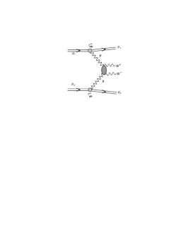
Figure 1: The general diagram for the $pp\to ppW^{+}W^{-}$ reaction via $\gamma\gamma\to W^{+}W^{-}$ subprocess.

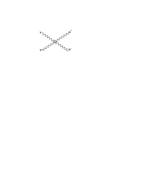
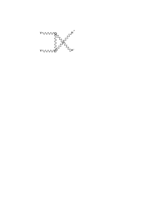
Figure 2: The leading order $\gamma\gamma\to W^{+}W^{-}$ subprocesses.

Then within the Standard Model, the elementary tree-level cross section for the $\gamma\gamma\to W^{+}W^{-}$ subprocess can be written in the very compact form in terms of the Mandelstam variables (see e.g. Ref. DDS95 )

$$\frac{d\hat{\sigma}}{d\Omega}=\frac{3\alpha^{2}\beta}{2\hat{s}}\left(1-\frac{2\hat{s}(2\hat{s}+3m_{W}^{2})}{3(m_{W}^{2}-\hat{t})(m_{W}^{2}-\hat{u})}+\frac{2\hat{s}^{2}(\hat{s}^{2}+3m_{W}^{4})}{3(m_{W}^{2}-\hat{t})^{2}(m_{W}^{2}-\hat{u})^{2}}\right)\,,$$ (2)

where $\beta=\sqrt{1-4m_{W}^{2}/\hat{s}}$ is the velocity of the $W$ bosons in their center-of-mass frame and the electromagnetic fine-structure constant $\alpha=e^{2}/(4\pi)\simeq 1/137$. The total elementary cross section can be obtained by integration of the differential cross section above.

III Exclusive $pp\to ppW^{+}W^{-}$ reaction

The $pp\to ppW^{+}W^{-}$ reaction is particularly interesting in the context of $\gamma\gamma WW$ coupling royon ; piotrzkowski .

In the Weizsäcker-Williams approximation, the total cross section for the $pp\to pp(\gamma\gamma)\to W^{+}W^{-}$ can be written as in the parton model:

$$\sigma=\int dx_{1}dx_{2}\,f_{1}^{WW}(x_{1})\,f_{2}^{WW}(x_{2})\,\hat{\sigma}_{\gamma\gamma\to W^{+}W^{-}}(\hat{s})\,.$$ (3)

We take the Weizsäcker-Williams equivalent photon fluxes in protons from Ref. DZ .

To calculate differential distributions the following parton formula can be conveniently used

$$\frac{d\sigma}{dy_{+}dy_{-}d^{2}p_{W\perp}}=\frac{1}{16\pi^{2}{\hat{s}}^{2}}\,x_{1}f_{1}^{WW}(x_{1})\,x_{2}f_{2}^{WW}(x_{2})\,\overline{|{\cal M}_{\gamma\gamma\to W^{+}W^{-}}(\hat{s},\hat{t},\hat{u})|^{2}}\,.$$ (4)

We shall not discuss here any approach beyond the Standard Model. A potentially interesting Higgsless scenario of the production of $W^{+}W^{-}$ pairs has been discussed previously e.g. in Refs. royon ; piotrzkowski .

The exclusive cross section could be calculated also more precisely in four-body calculation with corresponding $2\to 4$ matrix element. However, such a precision is not needed now when reviewing all potentially important contributions. This may become important for large statistics analysis of the 14 TeV data with extra measurement of forward protons and when discussing experimental cuts.

IV Inclusive production of $W^{+}W^{-}$ pairs

The dominant contribution of $W^{+}W^{-}$ pair production is initiated by quark-antiquark annihilation DDS95 . The gluon-gluon contribution to the inclusive cross section was calculated first in Ref. gg_WW .

Therefore for a comparison we also consider quark-antiquark and gluon-gluon components to the inclusive cross section. They will constitute a reference point for our calculations of the two-photon contributions.

IV.1 $q\bar{q}\to W^{+}W^{-}$ mechanism

The generic diagram for the $q\bar{q}$ initiated processes is shown in Fig.3. This contains $t$- and $u$-channel quark exchanges as well as $s$-channel photon and $Z$-boson exchanges DDS95 .

Figure 3: A generic diagram representing mechanisms for production of $W^{+}W^{-}$ pairs in the $q\bar{q}\to W^{+}W^{-}$ subprocess.

Therefore this process is also of interest as a probe of the gauge structure of the electroweak interactions. Relevant leading-order matrix element, averaged over quark colors and over initial spin polarizations and summed over final spin polarization, can be found e.g. in Ref. Eichten .

The corresponding differential cross section in leading-order approximation can be written as:

$$\frac{d\sigma}{dy_{+}dy_{-}d^{2}p_{W\perp}}=\frac{1}{16\pi^{2}{\hat{s}}^{2}}\,[x_{1}q(x_{1},\mu^{2})\,x_{2}{\bar{q}}(x_{2},\mu^{2})+x_{1}{\bar{q}}(x_{1},\mu^{2})\,x_{2}q(x_{2},\mu^{2})]\overline{|{\cal M}_{q{\bar{q}}\to W^{+}W^{-}}(\hat{s},\hat{t},\hat{u})|^{2}}\,.$$ (5)

IV.2 $gg\to W^{+}W^{-}$ mechanism

The generic diagram for the $gg$ initiated processes is shown in Fig.4. This contains both quark box diagrams and heavy-quark triangle with s-channel Higgs boson in the intermediate stage. More details of the relevant calculation can be found e.g. in Ref.LS2012 .

Figure 4: A generic diagram representing mechanisms for production of $W^{+}W^{-}$ pairs in the $gg\to W^{+}W^{-}$ subprocess.

The corresponding differential cross section corresponding to this contribution can be written as:

$$\frac{d\sigma}{dy_{+}dy_{-}d^{2}p_{W\perp}}=\frac{1}{16\pi^{2}{\hat{s}}^{2}}\,x_{1}g(x_{1},\mu^{2})\,x_{2}g(x_{2},\mu^{2})\overline{|{\cal M}_{gg\to W^{+}W^{-}}(\hat{s},\hat{t},\hat{u})|^{2}}\,.$$ (6)

This contribution is formally higher order in pQCD than the $q\bar{q}$ annihilation, but may be large numerically at higher energies when $x_{1}$ and $x_{2}$ become very small.

IV.3 $\gamma\gamma\to W^{+}W^{-}$ mechanism

In this section, we briefly discuss inclusive $\gamma\gamma\to W^{+}W^{-}$ mechanisms. We shall calculate that contribution to the inclusive $pp\to W^{+}W^{-}X$ process for the first time in the literature.

If at least one photon is a constituent of the nucleon then the mechanisms presented in Fig.5 are possible. In these cases at least one of participating proton does not survive the $W^{+}W^{-}$ production process. In the following we consider two different approaches to the problem.

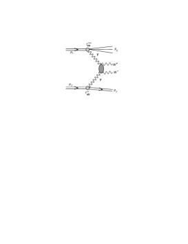
Figure 5: Diagrams representing inelastic photon-photon induced mechanisms for production of $W^{+}W^{-}$ pairs.

IV.3.1 Naive approach to photon flux

Some $\gamma\gamma$ induced processes ($\gamma\gamma\to H^{+}H^{-},L^{+}L^{-}$) were discussed long time ago in Ref.DGNR94 . In their approach the photon distribution in the proton is a convolution of the distribution of quarks in the proton and the distribution of photons in quarks/antiquarks

$$f_{\gamma/p}=f_{q}\otimes f_{\gamma/q}\;,$$ (7)

which can be written mathematically as

$$xf_{\gamma/p}(x)=\sum_{q}\int_{x}^{1}dx_{q}f_{q}(x_{q},\mu^{2})e_{q}^{2}\left(\frac{x}{x_{q}}\right)f_{\gamma/q}\left(\frac{x}{x_{q}},Q_{1}^{2},Q_{2}^{2}\right)\;,$$ (8)

where the sum runs over all quark and antiquark flavours. The flux of photons in a quark/antiquark in their approach was calculated as:

$$f_{\gamma}(z)=\frac{\alpha_{em}}{2\pi}\frac{1+(1-z)^{2}}{2}\log\left(\frac{Q_{1}^{2}}{Q_{2}^{2}}\right)\;.$$ (9)

The choice of scales in the formulae is a bit ambigous. They have proposed the following set of scales:

$$Q_{1}^{2} = \max({\hat{s}}/4-m_{W}^{2},1\mbox{GeV}^{2})$$

$$Q_{2}^{2} = 1\mbox{GeV}^{2}$$

$$\mu^{2} = {\hat{s}}/4\;.$$ (10)

We shall try to use the approach here as a reference for more refined calculation described in the next subsection.

IV.3.2 MRST-QED parton distributions

An improved approach how to include photons into inelastic processes was proposed some time ago by Martin, Roberts, Stirling and Thorne in Ref.MRST04 . In their approach photon is treated on the same footing as quarks, antiquarks and gluons. Below we repeat the essential points of their formalism which includes combined QCD+QED evolution.

They proposed a QED-corrected evolution equations for the parton distributions of the proton MRST04 :

$${\partial q_{i}(x,\mu^{2})\over\partial\log\mu^{2}} = {\alpha_{S}\over 2\pi}\int_{x}^{1}\frac{dy}{y}\Big{\{}P_{qq}(y)\;q_{i}(\frac{x}{y},\mu^{2})+P_{qg}(y)\;g(\frac{x}{y},\mu^{2})\Big{\}}\,$$

$$+ {\alpha\over 2\pi}\int_{x}^{1}\frac{dy}{y}\Big{\{}\tilde{P}_{qq}(y)\;e_{i}^{2}q_{i}(\frac{x}{y},\mu^{2})+P_{q\gamma}(y)\;e_{i}^{2}\gamma(\frac{x}{y},\mu^{2})\Big{\}},$$

$${\partial g(x,\mu^{2})\over\partial\log\mu^{2}} = {\alpha_{S}\over 2\pi}\int_{x}^{1}\frac{dy}{y}\Big{\{}P_{gq}(y)\;\sum_{j}q_{j}(\frac{x}{y},\mu^{2})+P_{gg}(y)\;g(\frac{x}{y},\mu^{2})\Big{\}},\,$$

$${\partial\gamma(x,\mu^{2})\over\partial\log\mu^{2}} = {\alpha\over 2\pi}\int_{x}^{1}\frac{dy}{y}\Big{\{}P_{\gamma q}(y)\;\sum_{j}e_{j}^{2}\;q_{j}(\frac{x}{y},\mu^{2})+P_{\gamma\gamma}(y)\;\gamma(\frac{x}{y},\mu^{2})\Big{\}}\;,$$ (11)

where

$${\tilde{P}}_{qq}=C_{F}^{-1}P_{qq}, P_{\gamma q}=C_{F}^{-1}P_{gq},$$

$$P_{q\gamma}=T_{R}^{-1}P_{qg}, P_{\gamma\gamma}=-\frac{2}{3}\;\sum_{i}e_{i}^{2}\;\delta(1-y)$$

The parton distributions in Eq.(11) fullfil the standard momentum sum rule:

$$\int_{0}^{1}dx\;x\;\Big{\{}\sum_{i}q_{i}(x,\mu^{2})+g(x,\mu^{2})+\gamma(x,\mu^{2})\Big{\}}=1\;.$$ (12)

IV.3.3 Cross section for photon-photon processes

In leading order corresponding triple differential cross section for inelastic-inelastic photon-photon contribution can be written as usually in the parton-model formalism:

$$\frac{d\sigma^{\gamma_{in}\gamma_{in}}}{dy_{1}dy_{2}d^{2}p_{t}} = \frac{1}{16\pi^{2}{\hat{s}}^{2}}x_{1}\gamma_{in}(x_{1},\mu^{2})\;x_{2}\gamma_{in}(x_{2},\mu^{2})\;\overline{|{\cal M}_{\gamma\gamma\to W^{+}W^{-}}|^{2}}\;.$$ (13)

The above contribution includes only cases when both nucleons do not survive the collision and nucleon debris is produced instead. The case when nucleon survives the collision has to be considered separately. In this case one can include corresponding photon distributions where extra ”el” index will be added to denote that physical situation. Corresponding contributions to the cross section can be then written as:

$$\frac{d\sigma^{\gamma_{in}\gamma_{el}}}{dy_{1}dy_{2}d^{2}p_{t}} = \frac{1}{16\pi^{2}{\hat{s}}^{2}}x_{1}\gamma_{in}(x_{1},\mu^{2})\;x_{2}\gamma_{el}(x_{2},\mu^{2})\;\overline{|{\cal M}_{\gamma\gamma\to W^{+}W^{-}}|^{2}}\;,$$

$$\frac{d\sigma^{\gamma_{el}\gamma_{in}}}{dy_{1}dy_{2}d^{2}p_{t}} = \frac{1}{16\pi^{2}{\hat{s}}^{2}}x_{1}\gamma_{el}(x_{1},\mu^{2})\;x_{2}\gamma_{in}(x_{2},\mu^{2})\;\overline{|{\cal M}_{\gamma\gamma\to W^{+}W^{-}}|^{2}}\;,$$

$$\frac{d\sigma^{\gamma_{el}\gamma_{el}}}{dy_{1}dy_{2}d^{2}p_{t}} = \frac{1}{16\pi^{2}{\hat{s}}^{2}}x_{1}\gamma_{el}(x_{1},\mu^{2})\;x_{2}\gamma_{el}(x_{2},\mu^{2})\;\overline{|{\cal M}_{\gamma\gamma\to W^{+}W^{-}}|^{2}}\;,$$ (14)

for inelastic-elastic, elastic-inelastic and elastic-elastic components, respectively. In the following the elastic photon fluxes are calculated using the Drees-Zeppenfeld parametrization DZ , where a simple parametrization of nucleon electromagnetic form factors is used.

IV.3.4 Resolved photons

So far we have discussed direct photonic contributions. In general, photon may also develop its hadronic structure. Then asymmetric diagrams with one photon attached to the upper or lower proton, as shown in Fig.6, become possible. Now extra photon remnant debris (called $X_{\gamma,1}$ or $X_{\gamma,2}$ in the figure) appears in addition. One may expect that such diagrams lead to quite asymmetric distributions in rapidity of $W$ bosons with maxima in forward and/or backward directions.

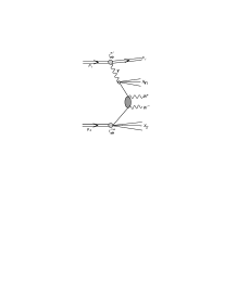
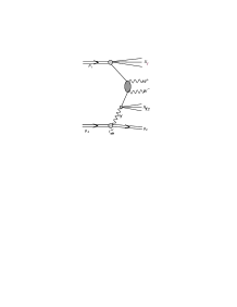
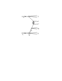
Figure 6: Diagrams representing some single resolved photon mechanisms with quark-antiquark annihilation for production of $W^{+}W^{-}$ pairs. There exist also similar diagrams with gluon-gluon subprocesses.

Another type of diagrams with resolved photons is shown in Fig.7. We expect the contributions of the second category of diagrams, shown in Fig.7, to be rather small.

Figure 7: Diagrams representing mechanisms with two resolved photons for production of $W^{+}W^{-}$ pairs.

In the case of resolved photons, the “photonic” quark/antiquark distributions in a proton must be calculated first. This can be done as the convolution

$$f_{q/p}^{\gamma}=f_{\gamma/p}\otimes f_{q/\gamma}$$ (16)

which mathematically means:

$$xf_{q/p}^{\gamma}(x)=\int_{x}^{1}dx_{\gamma}f_{\gamma/p}(x_{\gamma},\mu_{s}^{2})\left(\frac{x}{x_{\gamma}}\right)f\left(\frac{x}{x_{\gamma}},\mu_{h}^{2}\right)\;.$$ (17)

Technically first $f_{\gamma/p}$ in the proton is prepared on a dense grid for $\mu_{s}^{2}\sim$ 1 GeV² (virtuality of the photon) and then is used in the convolution formula (17). The second scale is evidently hard $\mu_{h}^{2}\sim M_{WW}^{2}$. The result strongly depends on the choice of the soft scale $\mu_{s}^{2}$. In this sense our calculations are not very precise and must be treated rather as a rough estimate. The new quark/antiquark distributions of photonic origin are used to calculate cross section as for the standard quark-antiquark annihilation subprocess.

IV.4 Single diffractive production of $W^{+}W^{-}$ pairs

In the following we apply the resolved pomeron approach IS_ee ; IS_ccbar . In this approach one assumes that the Pomeron has a well defined partonic structure, and that the hard process takes place in a Pomeron–proton or proton–Pomeron (single diffraction) or Pomeron–Pomeron (central diffraction) processes. The mechanism of single diffractive production of $W^{+}W^{-}$ pairs is shown in Fig.8. We calculate triple differential distributions

$${d\sigma_{SD}^{(1)}\over dy_{1}dy_{2}dp_{t}^{2}}={\Big{|}M\Big{|}^{2}\over 16\pi^{2}\hat{s}^{2}}\,\Big{[}\,\Big{(}x_{1}q_{f}^{D}(x_{1},\mu^{2})\,x_{2}\bar{q}_{f}(x_{2},\mu^{2})\Big{)}\,+\Big{(}x_{1}\bar{q}_{f}^{D}(x_{1},\mu^{2})\,x_{2}q_{f}(x_{2},\mu^{2})\Big{)}\,\Big{]},$$

(18)

$${d\sigma_{SD}^{(2)}\over dy_{1}dy_{2}dp_{t}^{2}}={\Big{|}M\Big{|}^{2}\over 16\pi^{2}\hat{s}^{2}}\,\Big{[}\,\Big{(}x_{1}q_{f}(x_{1},\mu^{2})\,x_{2}\bar{q}_{f}^{D}(x_{2},\mu^{2})\Big{)}\,+\Big{(}x_{1}\bar{q}_{f}(x_{1},\mu^{2})\,x_{2}q_{f}^{D}(x_{2},\mu^{2})\Big{)}\,\Big{]},$$

(19)

$${d\sigma_{CD}\over dy_{1}dy_{2}dp_{t}^{2}}={\Big{|}M\Big{|}^{2}\over 16\pi^{2}\hat{s}^{2}}\,\Big{[}\,\Big{(}x_{1}q_{f}^{D}(x_{1},\mu^{2})\,x_{2}\bar{q}_{f}^{D}(x_{2},\mu^{2})\Big{)}\,+\Big{(}x_{1}\bar{q}_{f}^{D}(x_{1},\mu^{2})\,x_{2}q_{f}^{D}(x_{2},\mu^{2})\Big{)}\,\Big{]}$$

(20)

for single-diffractive and central-diffractive production, respectively. The matrix element squared for the $q\bar{q}\to W^{+}W^{-}$ process is the same as previously discussed for the nondiffractive processes.

In this approach longitudinal momentum fractions are calculated as

$$x_{1}={m_{t}\over\sqrt{s}}\Big{(}e^{y_{2}}+e^{y_{2}}\Big{)},$$ (21)

$$x_{2}={m_{t}\over\sqrt{s}}\Big{(}e^{-y_{1}}+e^{-y_{2}}\Big{)}$$

with $m_{t}=\sqrt{(p_{t}^{2}+m_{W}^{2})}\approx p_{t}$. The distribution in the $WW$ invariant mass can be obtained by binning differential cross section in $M_{WW}$.

In the present analysis we consequently do not calculate higher-order contributions. In principle, they could be included effectively with the help of a so-called $K$-factor.

The ’diffractive’ quark/antiquark distribution of flavour $f$ can be obtained by a convolution of the flux of Pomerons $f_{\bf I\!P}(x_{\bf I\!P})$ and the parton distribution in the Pomeron $q_{f/{\bf I\!P}}(\beta,\mu^{2})$:

$$q_{f}^{D}(x,\mu^{2})=\int dx_{\bf I\!P}d\beta\,\delta(x-x_{\bf I\!P}\beta)q_{f/{\bf I\!P}}(\beta,\mu^{2})\,f_{\bf I\!P}(x_{\bf I\!P})\,=\int_{x}^{1}{dx_{\bf I\!P}\over x_{\bf I\!P}}\,f_{\bf I\!P}(x_{\bf I\!P})q_{f/{\bf I\!P}}({x\over x_{\bf I\!P}},\mu^{2})\,.$$

(22)

The flux of Pomerons $f_{\bf I\!P}(x_{\bf I\!P})$ enters in the form integrated over four–momentum transfer

$$f_{\bf I\!P}(x_{\bf I\!P})=\int_{t_{min}}^{t_{max}}dt\,f(x_{\bf I\!P},t)\,,$$ (23)

with $t_{min},t_{max}$ being kinematic boundaries.

Both pomeron flux factors $f_{{\bf I\!P}}(x_{{\bf I\!P}},t)$ as well as quark/antiquark distributions in the pomeron are taken from the H1 collaboration analysis of diffractive structure function and diffractive dijets at HERA H1 . The factorization scale for diffractive parton distributions is taken as $\mu^{2}=M_{WW}^{2}$.

In the present analysis we consider both pomeron and subleading reggeon contributions. The corresponding diffractive quark distributions are obtained by replacing pomeron flux by the reggeon flux and quark/antiquark distributions in the pomeron by their counterparts in subleading reggeon(s). The other details can be found in H1 . In the case of pomeron exchange the upper limit in (22) is 0.1 and for reggeon exchange 0.2. In our opinion, the whole Regge formalism does not apply above these limits.

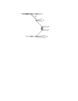
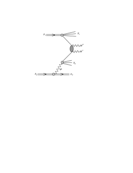
Figure 8: Diagrams representing single diffractive mechanism of production of $W^{+}W^{-}$ pairs.

Up to now we have assumed Regge factorization which is known to be violated in hadron-hadron collisions. It is known that these are soft interactions which lead to an extra production of particles which fill in the rapidity gaps related to pomeron exchange.

Different models of absorption corrections (one-, two- or three-channel approaches) for diffractive processes were presented in the literature. The absorption effects for the diffractive processes were calculated e.g. in Ref Khoze ; Maor . The different models give slightly different predictions. Usually an average value of the gap survival probability $<|S|^{2}>$ is calculated first and then the cross sections for different processes is multiplied by this value. We shall follow this somewhat simplified approach also here. Numerical values of the gap survival probability can be found in Khoze ; Maor . The survival probability depends on the collision energy. It is sometimes parametrized as:

$$<|S|^{2}>(\sqrt{s})=\frac{a}{b+\ln(\sqrt{s})}\;.$$ (24)

The numerical values of the parameters can be found in original publications. In general, the absorptive corrections for single and central diffractive processes are somewhat different.

IV.5 Double parton scattering

The diagram representating the double parton scattering process is shown in Fig.9.

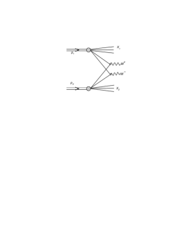
Figure 9: Diagram representing double parton scattering mechanism of production of $W^{+}W^{-}$ pairs.

The cross section for double parton scattering is often modelled in the factorized anzatz which in our case would mean:

$$\sigma_{W^{+}W^{-}}^{DPS}=\frac{1}{\sigma_{qq}^{eff}}\sigma_{W^{+}}\sigma_{W^{-}}\;.$$ (25)

In general, the parameter $\sigma_{qq}$ does not need to be the same as for gluon-gluon initiated processes $\sigma_{gg}^{eff}$. In the present, rather conservative, calculations we take it to be $\sigma_{qq}^{eff}=\sigma_{gg}^{eff}$ = 15 mb. The latter value is known within about 10 % from systematics of gluon-gluon initiated processes at the Tevatron and LHC.

The factorized model (25) can be generalized to more differential distributions (see e.g. LMS2012 ; MS2013 ). For example in our case of $W^{+}W^{-}$ production the cross section differential in $W$ boson rapidities can be written as:

$$\frac{d\sigma_{W^{+}W^{-}}^{DPS}}{dy_{+}dy_{-}}=\frac{1}{\sigma_{qq}^{eff}}\frac{d\sigma_{W}^{+}}{dy_{+}}\frac{d\sigma_{W}^{-}}{dy_{-}}\;.$$ (26)

In particular, in leading-order approximation the cross section for quark-antiquark annihilation reads:

$$\frac{d\sigma}{dy}=\sum_{ij}\left(x_{1}q_{i/1}(x_{1},\mu^{2})x_{2}{\bar{q}}_{j/2}(x_{2},\mu^{2})+x_{1}{\bar{q}}_{i/1}(x_{1},\mu^{2})x_{2}q_{j/2}(x_{1},\mu^{2})\right)\overline{|{\cal M}_{ij\to W^{\pm}}|^{2}}\;,$$ (27)

where the matrix element for quark-antiquark annihilation to $W$ bosons (${\cal M}_{ij\to W^{\pm}}$) contains Cabibbo-Kobayashi-Maskawa matrix elements. In the present paper for illustration we shall show the $\frac{d\sigma}{dy_{+}dy_{-}}$, as well as distributions in rapidity distance between $W^{+}$ and $W^{-}$ and distribution in $M_{WW}$. In the approximations made here (leading order approximation, no transverse momenta of W bosons)

$$M_{WW}^{2}=2M_{W}^{2}\left(1+\mbox{cosh}(y_{1}-y_{2})\right)\;.$$ (28)

When calculating the cross section for single $W$ boson production in leading-order approximation a well known Drell-Yan $K$-factor can be included. The double-parton scattering would be then multiplied by $K^{2}$.

V Results

Before a detailed survey of results of the different contributions discussed in the present paper let us concentrate on some technical details concerning inelastic photon-photon contributions. In Fig.11 we show rapidity distributions for the naive (left panel) and QCD improved (right panel) approaches discussed in section IV. While in the naive approximation the elastic-elastic component is the largest and inelastic-inelastic is the smallest, in the QCD improved approach the situation is reversed. Here in the QCD improved calculations $\mu_{F}^{2}=M_{WW}^{2}$ was used as the factorization scale.

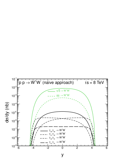
Figure 10: Rapidity distribution of $W$ bosons for $\sqrt{s}$ = 8 TeV. The left panel shows results for the naive approach often used in the past, while the right panel shows the result with the QCD improved method proposed in Ref.MRST04 .

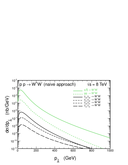
Figure 11: Transverse momentum distribution of $W$ bosons for $\sqrt{s}$ = 8 TeV. The left panel shows results for the naive approach often used in the past, while the right panel shows the result with the QCD improved method proposed in Ref.MRST04 .

For the searches of anomalous $\gamma\gamma WW$ coupling the ratios of inelastic-inelastic, elastic-inelastic and inelastic-elastic to elastic-elastic one are very useful. In Fig.12 and 13 we show such ratios in rapidity and transverse momentum of $W$ bosons. In the naive approach the ratios are smaller than 1 except of some small corners of the phase-space. In the QCD improved approach the ratios become much bigger. In particular, the ratio for inelastic-inelastic contribution is order of magnitude larger than 1.

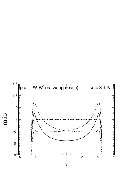
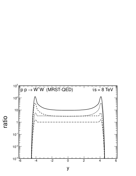
Figure 12: The ratio of elastic-inelastic (dashed), inelastic-elastic (dotted), inelastic-inelastic (dash-dotted) and all inelastic (solid) to the elastic-elastic cross section as a function of $W$ boson rapidity.

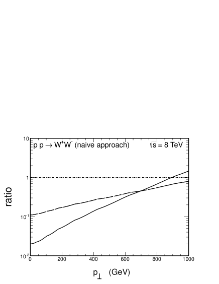
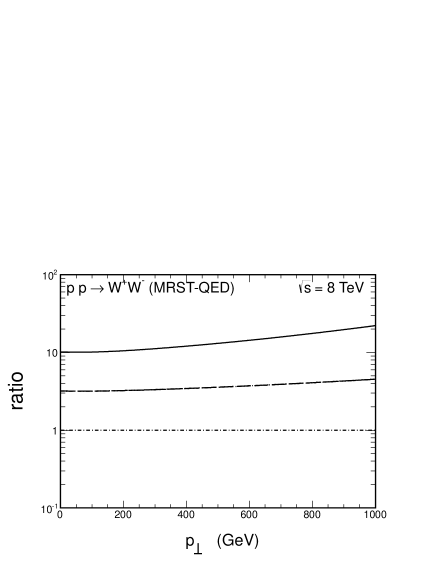
Figure 13: The ratio of elastic-inelastic (dashed), inelastic-elastic (dotted), inelastic-inelastic (dash-dotted) and all inelastic (solid) to the elastic-elastic cross section as a function of $W$ boson transverse momentum.

Now we wish to present a systematic survey of all the contributions discussed in the present paper.

The distribution in $W$ boson rapidity is shown in Fig.14. We show separate contributions discussed in the present paper. The diffractive contribution is an order of magnitude larger than the resolved photon contribution. The estimated reggeon contribution is of similar size as the pomeron contribution. The distributions of $W^{+}$ and $W^{-}$ for double-parton scattering contribution are different and reflect distribution and, in the approximation discussed here, have shapes identical as for single production of $W^{+}$ and $W^{-}$, respectively. It would be therefore interesting to obtain separate distributions for $W^{+}$ and $W^{-}$ experimentally. This is, however, a rather difficult task. Distributions of charged leptons (electrons, muons) could also be interesting in this context.

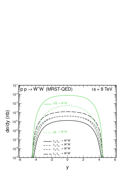
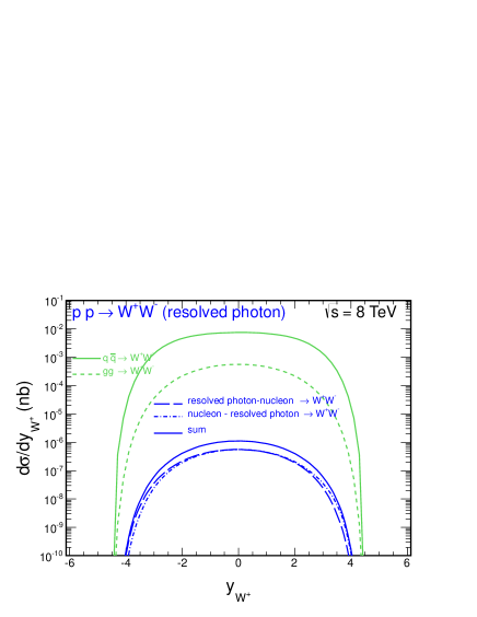
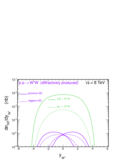
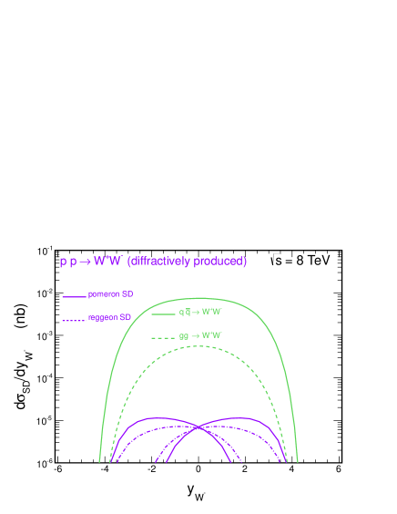
Figure 14: Rapidity distribution of $W$ bosons for $\sqrt{s}$ = 8 TeV. The top panel shows contributions of all photon-photon induced processes, the middle panels resolved photon contributions and the bottom panels distributions of the diffractive contribution. The diffractive cross section has been multiplied by the gap survival factor $S_{G}^{2}$ = 0.03.

In Fig.15 we present distribution in transverse momentum of $W$ bosons. All photon-photon components have rather similar shapes. The photon-photon contributions are somewhat harder than those for diffractive and resolved photon mechanisms.

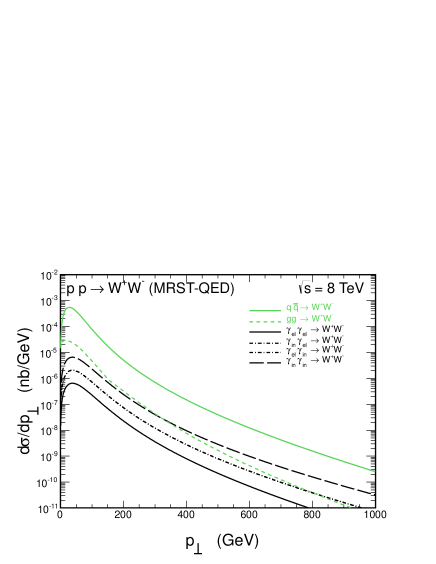
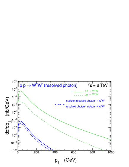
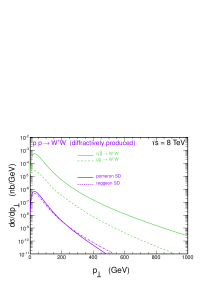
Figure 15: Transverse momentum distribution of $W$ bosons for $\sqrt{s}$ = 8 TeV. The left-top panel shows all photon-photon induced processes, the right-top panel resolved photon contributions and the bottom panel the diffractive contribution. The diffractive cross section has been multiplied by the gap survival factor $S_{G}^{2}=$ 0.03.

In Fig.16 we show distributions in invariant mass of the $WW$ pairs. The relative contributions of the photon-photon and DPS components clearly grow with the invariant mass. The same would be true for the distribution in the rapidity distance between the gauge bosons. In reality one rather measures charged leptons. Then the distributions in invariant mass of positive and negative leptons or in rapidity distance between them would be interesting. This requires a dedicated study in the future.

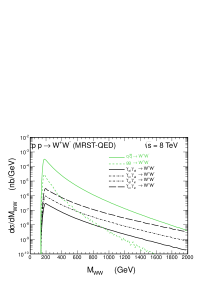
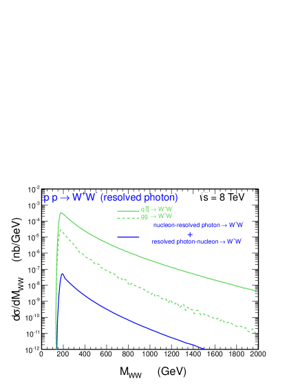
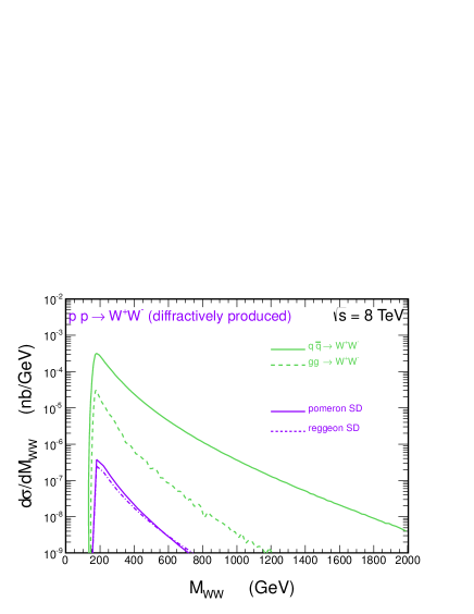
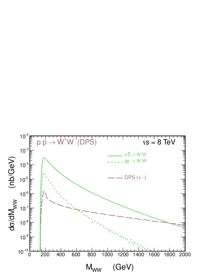
Figure 16: Distribution in invariant mass of the $WW$ pairs for $\sqrt{s}$ = 8 TeV. The top-left panel shows contributions of all photon-photon induced processes, the top-right panel resolved photon contributions, the bottom-left panel the contributions of diffractive process and the bottom-right panel the contribution of DPS. The diffractive cross section has been multiplied by the gap survival factor $S_{G}^{2}$ = 0.03.

Finally, for completeness, in Fig.17 we present some interesting examples of two-dimensional distributions in rapidity of $W^{+}$ and $W^{-}$. We show three different distributions for the dominant $q\bar{q}$, inelastic-inelastic photon-photon and double-parton scattering components. The $q\bar{q}$ component dominates at $y_{1},y_{2}\approx$ 0. The photon-photon component has “broader” distribution in $y_{1}$ and $y_{2}$. In contrast, the double-parton scattering component gives a very flat two-dimensional distribution. The information presented in the figure can be used in order to “enhance” content of the interesting component. A study of leptons from the $W$-boson decays would be a next interesting step in understanding practical possibilities to study the different components discussed here at the LHC.

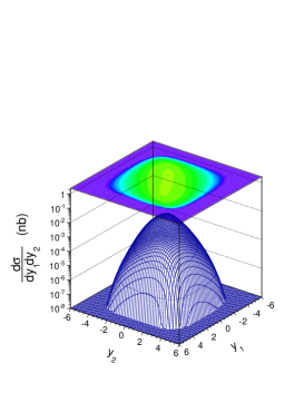
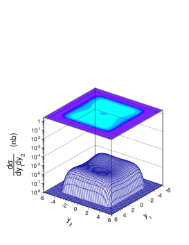
Figure 17: Two dimensional distributions in rapidity of $W^{+}$ and rapidity of $W^{-}$ for the dominant $q\bar{q}$ (left), inelastic-inelastic photon-photon (middle) and double-parton scattering (right) contributions at $\sqrt{s}$ = 8 TeV.

The general situation is summarized in Table 1. The photon-photon induced processes give quite large contribution. The single-resolved photon contributions are at least order of magnitude smaller than the diffractive contribution. This is still surprisingly large. The reason that the single resolved photon contributions are relatively large is due to the fact that quark or antiquark carry on average fairly large fraction of the photon longitudinal momentum. The double parton scattering contribution is not too large. It may be, however, important for large rapidity distances between gauge bosons. The diffractive contributions in the table are not multiplied by the gap survival factor ($S^{2}_{G}$) which is known only approximately. The single-diffractive contributions have rather different shape in rapidity than the resolved-photon contributions in spite of topological similarity.

In real experiments only rather limited part of the phase space is covered. The total cross section is then obtained by extrapolation into unmeasured region with the help of Monte Carlo codes. It is needless to say that none of the new contributions discussed here is included when extrapolating purely experimental results to the phase-space integrated cross sections. This means that the “measured” total cross section is underestimated. In order to answer the question “how much” requires dedicated Monte Carlo analyses.

Table 1: Contributions of different subleading processes discussed in the present paper to the total cross section for different energies. The cross section is given in pb. The diffractive contributions here have not been multiplied by the gap survival factor. The combinatorial factor 1/2 is shown explicitly for the double parton scattering (DPS) contribution for $W^{+}W^{+}$ and $W^{-}W^{-}$ final states shown for completeness. .

contribution	1.96 TeV	7 TeV	8 TeV	14 TeV	comment
CDF	12.1 pb
D0	13.8 pb
ATLAS		54.4 pb			large extrapolation
CMS		41.1 pb			large extrapolation
$q\bar{q}$	9.86	27.24	33.04	70.21	dominant (LO, NLO)
$gg$	5.17 10-2	1.48	1.97	5.87	subdominant (NLO)
$\gamma_{el}\gamma_{el}$	3.07 10-3	4.41 10-2	5.40 10-2	1.16 10-1	new, anomalous $\gamma\gamma WW$
$\gamma_{el}\gamma_{in}$	1.08 10-2	1.40 10-1	1.71 10-1	3.71 10-1	new, anomalous $\gamma\gamma WW$
$\gamma_{in}\gamma_{el}$	1.08 10-2	1.40 10-1	1.71 10-1	3.71 10-1	new, anomalous $\gamma\gamma WW$
$\gamma_{in}\gamma_{in}$	3.72 10-2	4.46 10-1	5.47 10-1	1.19	anomalous $\gamma\gamma WW$
$\gamma_{el,res}-q/\bar{q}$	1.04 10-4	2.94 10-3	3.83 10-3	1.03 10-2	new, rather sizeable
$q/\bar{q}-\gamma_{el.res}$	1.04 10-4	2.94 10-3	3.83 10-3	1.03 10-2	new, rather sizeable
$\gamma_{in,res}-q/\bar{q}$					not calculated
$q/\bar{q}-\gamma_{in.res}$					not calculated
DPS(++)	0.61 10${}^{-2}/2$	0.22/2	0.29/2	1.02/2	not included in NLO
DPS(- -)	0.58 10${}^{-2}/2$	0.76 10${}^{-1}/2$	0.11/2	0.40/2	not included in NLO
DPS(+-)	0.6 10-2	0.13	0.18	0.64	not included in NLO
DPS(-+)	0.6 10-2	0.13	0.18	0.64	not included in NLO
${\bf I\!P}p$ $(x_{{\bf I\!P}}<0.1)$	2.82 10-2	9.88 10-1	1.27	3.35	new, relatively large
$p{\bf I\!P}$ $(x_{{\bf I\!P}}<0.1)$	2.82 10-2	9.88 10-1	1.27	3.35	new, relatively large
${\bf I\!R}p$ $(x_{{\bf I\!R}}<0.2)$	4.51 10-2	7.12 10-1	8.92 10-1	2.22	new, relatively large
$p{\bf I\!R}$ $(x_{{\bf I\!R}}<0.2)$	4.51 10-2	7.12 10-1	8.92 10-1	2.22	new, relatively large

Some comments on recent studies on $\gamma\gamma W^{+}W^{-}$ boson couplings, as performed recently by the D0 and CMS collaborations gamgam_WW_D0 ; gamgam_WW_CMS are in order. In the D0 collaboration analysis the inelastic contributions are not included when extracting limits on anomalous couplings. The CMS collaboration requires an extra condition of no charged particles in the central pseudorapidity interval. When comparing calculations to the experimental data the inelastic contributions are estimated by rescalling elastic-elastic contribution by an experimental function depending on kinematical variables (invariant mass, transverse momentum of the $\mu^{+}\mu^{-}$ pair) obtained in the analysis of $\mu^{+}\mu^{-}$ continuum. It is not clear to us whether such a procedure is consistent for $W^{+}W^{-}$ production, where leptons come from decays of the gauge bosons and invariant mass and transverse moemtum of the $W^{+}W^{-}$ pair is very different than invariant mass and transverse momentum of the corresponding dimuons. This cannot be checked in the present approach with collinear photons and requires inclusion of photon transverse momenta. Within the present approach we predict that inelastic contributions are significantly larger than the elastic-elastic one. The fragmentation of the remnants of inelastic excitations is needed to understand to which extend the inelastic contributions survive the veto condition. One can expect that particles from the fragmentation of the proton remnants after the photon emission are emitted in rather forward/backward directions. The $D0$ collaboration also neglects the inelastic contribution when calculating the Standard Model background at large lepton transverse momenta, in spite they have no explicit veto condition on charge particles. Inclusion of photon-photon inelastic contributions would therefore lower considerably their lower limits on parameters of models with anomalous quartic $\gamma\gamma WW$ coupling. The diffractive contributions could also contribute to the distributions measured by the CMS and D0 collaborations. Clearly further analyses that focus on final states of proton remnants (after photon emission) are necessary.

VI Conclusions

In the present paper we have calculated for the first time a complete set of photon-photon and photon-(anti)quark and (anti)quark-photon contributions to the inclusive production of $W^{+}W^{-}$ pairs.

The photon-photon contributions can be classified into four topological categories: elastic-elastic, elastic-inelastic, inelastic-elastic and inelastic-inelastic, depending whether proton(s) survives the emission of the photon or not. The photon-photon contributions were calculated as done in the past e.g. for production of pairs of charged Higgs bosons or pairs of heavy leptons beyond Standard Model, and within QCD-improved method using MRST(QED) parton distributions. The second approach was already applied to the production of Standard Model charged lepton pair production and $c\bar{c}$ production. In the first approach we have obtained: $\sigma_{ela,ela}>\sigma_{ela,ine}=\sigma_{ine,ela}>\sigma_{ine,ine}$. In the more refined second approach we have got $\sigma_{ela,ela}<\sigma_{ela,ine}=\sigma_{ine,ela}<\sigma_{ine,ine}$. The two approaches give quite different results. In the first (naive) approach the inelastic-inelastic contribution is considerably smaller than elastic-inelastic or inelastic-elastic. In the approach when photon distribution in the proton undergoes QCD $\otimes$ QED evolution, it is the inelastic-inelastic contribution which is the biggest out of the four contributions. This shows that including photon into evolution equation is crucial. This is also a lesson for other processes known from the literature, where photon-photon processes are possible. This includes also some processes beyond the Standard Model mentioned in this paper.

The inelastic contributions sum up to the cross section of the order of 0.5 - 1 pb at the LHC energies. The photon-photon contributions are particularly important at large $WW$ invariant masses, i.e. probably also large invariant masses of charged leptons where its contribution is larger than that for gluon-gluon fusion.

The elastic-inelastic or inelastic-elastic contributions are interesting by themselves. Since they are related to the emission of forward/backward protons they could be potentially measured in the future with the help of forward proton detectors. Both CMS and ATLAS have plans for installing such detectors after the present (2013-2014) shutdown. Unfortunately the mechanisms are expected to have similar topology of the final state as single-diffractive contributions to $W^{+}W^{-}$ production. It would be therefore valuable to make a dedicated study how to pin down the mixed elastic-inelastic contributions. Clearly this would be a valuable test of both the formalism presented and our understanding of the underlying reaction mechanism.

We have discussed also briefly the double-scattering mechanism which also significantly contributes to large $M_{WW}$ invariant masses. This was suggested recently as an important ingredient for the Higgs background in the $WW^{*}$ or $ZZ^{*}$ final channels. Our estimate is more than order of magnitude smaller than that suggested recently in the literature in order to explain the Higgs signal in the $W^{+}W^{-}$ channel.

After this paper was completed we have learned about a detailed study of uncertainties of a photon PDF in the framework of so-called neural network PDFs NNPDF . This analysis suggests that inelastic photon-induced contributions may have rather big uncertainies. The issue should be better clarified in the future by comparing similar calculation for two-photon-induced $\mu^{+}\mu^{-}$ production at large invariant masses of dileptons to appropriate experimental data.

Acknowledgments

We are indebted to Krzysztof Piotrzkowski, Jonathan Hollar, and Gustavo da Silveira for a discussion of the CMS experiment on semi-exclusive production of $W^{+}W^{-}$ pairs and Christophe Royon, Sudeshna Banerjee and Emilien Chapon for the discussion of the D0 studies on $\gamma\gamma WW$ anomalous coupling. The help of Piotr Lebiedowicz in calculating the gluon-gluon component is acknowleded. We are indebted to Wolfgang Schäfer for a FORTRAN routine and an interesting discussion. We are indebted to Stefano Forte and Juan Rojo for a communication on their recent work on photon NNPDF. This work was partially supported by the Polish MNiSW grant DEC-2011/01/B/ST2/04535 and by the bilateral exchange program between Polish Academy of Sciences and FNRS, Belgium.

References

-
(1)
O. Kepka and C. Royon, Phys. Rev. D78 (2008) 073005;
E. Chapon, C. Royon and O. Kepka, Phys. Rev. D81 (2010) 074003. -
(2)
N. Schul and K. Piotrzkowski, Nucl. Phys. B (Proc. Suppl.) 179-180 (2008) 289;
T. Pierzchała and K. Piotrzkowski, Nucl. Phys. B (Proc. Suppl.) 179-180 (2008) 257. - (3) P. Lebiedowicz, R. Pasechnik and A. Szczurek, Phys. Rev. D81 (2012) 036003.
-
(4)
B.E. Cox et al.,
Eur. Phys. J. C45 (2006) 401;
S. Heinemeyer et al., Eur. Phys. J. C53 (2008) 231. - (5) R.S. Gupta, Phys. Rev. D85 (2012) 014006.
-
(6)
CMS and TOTEM diffractive and forward physics working group,
CERN/LHCC 2006-039/G-124, CMS Note 2007/002, TOTEM Note 06-5,
December 2006;
M. Albrow et al. (FP420 R and D Collaboration), JINST 4 (2009) T10001 [arXiv:0806.0302 [hep-ex]];
The AFP project in ATLAS, Letter of Intent of the PhaseI Upgrade (ATLAS Collaboration), http://cdsweb.cern.ch/record/1402470;
C. Royon (RP220 Collaboration), arXiv:0706.1796 [physics.ins-det];
M. Tasevsky, Nucl. Phys. Proc. Suppl. 179-180 (2008) 187;
The PPS upgrade project in CMS, M. Albrow, AIP Conf. Proc. 1523 (2012) 320. - (7) CMS Collaboration, Phys. Lett. B699 (2011) 25.
- (8) ATLAS Collaboration, arXiv:1203.6232 [hep-ex].
- (9) A. Kulesza and W.J. Stirling, Phys. Lett. B475 (2000) 168.
- (10) J.R. Gaunt, Ch.-H. Kom, A. Kulesza and W.J. Stirling, arXiv:1003.3953 [hep-ph].
- (11) J.R. Gaunt, Ch.-H. Kom, A. Kulesza and W.J. Stirling, arXiv:1110.1174 [hep-ph].
- (12) W. Krasny and W. Płaczek, arXiV:1305.1769 [hep-ph].
- (13) CMS Collaboration, arXiv:1305.5596 [hep-ex].
- (14) D0 Collaboration, arXiv:1305.1258 [hep-ex].
-
(15)
A. Bierweiler, T. Kasprzik, H. Kühn and S. Uccirati, JHEP 1211 (2012)
093;
A. Bierweiler, T. Kasprzik and J.H. Kühn, arXiv:1305.5402;
J. Baglio, Le Duc Ninh and M.M. Webber, arXiv:1307.4331. - (16) G. Aad et al. [ATLAS Collaboration], Phys. Lett. B716, 1 (2012); Science 338, 1576 (2012).
- (17) S. Chatrchyan et al. [CMS Collaboration], Phys. Lett. B716, 30 (2012); Science 338, 1569 (2012).
-
(18)
J. Ohnemus, Phys. Rev. D44 (1991) 3477;
S. Frixione, P. Nason and G. Ridolfi, Nucl. Phys. B383 (1992) 3;
S. Frixione, Nucl. Phys. B410 (1993) 280;
L.J. Dixon, Z. Kunszt and A. Signer, Nucl. Phys. B531 (1998) 3;
J.M. Campbell, R.K. Ellis, Phys. Rev. D60 (1999) 113006. - (19) A. Denner, S. Dittmaier and R. Schuster, Nucl. Phys. B452 (1995) 80.
- (20) M. Drees and D. Zeppenfeld, Phys. Rev. D39 (1989) 2536.
-
(21)
D.A. Dicus, C. Kao and W. Repko, Phys. Rev. D36 (1987) 1570;
E.N. Glover and J. van der Bij, Phys. Lett. B219 (1989) 488;
E.N. Glover and J. van der Bij, Nucl. Phys. B321 (1989) 561. - (22) E. Eichten, L. Hinchliffe, K. Lane, C. Quigg, Rev. Mod. Phys. 56 (1984) 579.
- (23) M. Drees, R.M. Godbole, M. Nowakowski and S.D. Rindani, Phys. Rev. D94 (1994) 2335.
- (24) A.D. Martin, R.G. Roberts, W.J. Stirling, R.S. Thorne, Eur.Phys.J.C39:155-161,2005
- (25) G. Kubasiak and A. Szczurek, Phys. Rev. D84 (2011) 014005.
- (26) M. Łuszczak, R. Maciuła and A. Szczurek, Phys. Rev. D84 (2011) 114018.
- (27) A. Aktas et al. [H1 Collaboration], Eur. Phys. J. C 48, 715 (2006) [arXiv:hep-exp/0606004].
- (28) V.A. Khoze, A.D. Martin and M.G. Ryskin, Eur. Phys. J. C18 (2000) 167.
- (29) U. Maor, AIP Conf. Proc. 1105 (2009) 248.
- (30) M. Łuszczak, R. Maciuła and A. Szczurek, Phys. Rev. D85 (2012) 094034.
- (31) R. Maciuła and A. Szczurek, Phys. Rev. D87 (2013) 074039.
- (32) R.D. Ball, V. Bertone, S. Carrazza, L. Del Debbio, S. Forte, A. Guffanti, N.P. Harltland and J. Rojo, arXiv:1308.0598.