Computation of Large Deviation Statistics via Iterative Measurement-and-Feedback Procedure

Takahiro Nemoto and Shin-ichi Sasa Division of Physics and Astronomy, Graduate School of Science, Kyoto University, Kyoto 606-8502, Japan
Abstract

We propose a computational method for large deviation statistics of time-averaged quantities in general Markov processes. In our proposed method, we repeat a response measurement against external forces, where the forces are determined by the previous measurement as feedback. Consequently, we obtain a set of stationary states corresponding to an exponential family of distributions, each of which shows rare events in the original system as the typical behavior. As a demonstration of our method, we study large deviation statistics of one-dimensional lattice gas models.

pacs:
05.40.-a, 05.10.-a, 05.70.Ln

Introduction.β€”Rare events, which are hardly observed, sometimes lead to substantial effects in nature. Examples may be seen in a broad range of phenomena including biomolecular reactions, nucleation, and plate-tectonic activities. Although understanding the statistical behavior of such rare events may be an important problem, it turns out from the definition that direct observation of rare events is too difficult. Remarkably, several techniques have been invented for generating rare events in numerical simulations, such as transition path sampling Frenkel ; Chandler , transition interface sampling Erp ; Erp2 , forward flux sampling Allen ; Allen2 , and the population dynamics method Populationdynamics ; Populationdynamics2 . However, contrary to the progress made with respect to numerical simulations, there are no methods that facilitate the observation of rare events in laboratory systems. Our final goal is to construct a rare-event sampling method that can be useful in laboratory experiments. Toward this end, in the present Letter, for rare events characterized by large deviation statistics, we efficiently calculate the frequencies of the rare events via an iterative measurement-and-feedback procedure, which might be implemented in laboratory experiments.

We here formulate the large deviation statistics. For a time-dependent quantity $x(t)$, we consider the time-averaged value $X(\tau)=(1/\tau)\int_{0}^{\tau}dtx(t)$, where $\tau$ denotes the averaging time. According to the law of large numbers, as we increase $\tau$, the deviation of $X(\tau)$ from the expected value $X_{0}$ decreases. However, even for large values of $\tau$, when we perform the same measurement many times, certain obtained values will deviate from the typical value $X_{0}$. The large deviation principle, which is proved in many systems Dembo_Zeitouni ; Touchette , is a law that claims the asymptotic form of the probability density in the limit $\tau\rightarrow\infty$ to be $e^{-\tau I(X)}$. Here, the function $I(X)$, which characterizes the statistical properties of those rare events, is called a large deviation function.

While studies of large deviation functions have a long history in probability theory, the functions have attracted attention in the field of nonequilibrium physics particularly in the last two decades. Since the discovery of the fluctuation theorem, which is the symmetry property of the large deviation function of the time-averaged entropy production rate FT ; FT2 , several results for large deviation functions have been found, such as an additivity principle for driven diffusive systems BD ; BD2 , dynamical phase transitions of kinetically constrained models garrahan ; garrahan2 , a Lyapunov function for nonequilibrium steady states without relying on entropy production CMaes , exact results for the current statistics of lattice gas models Gorissen ; Gorissen2 , and formulas motivated by the formal correspondence between large deviation functions and thermodynamic functions Evans ; JackSollich ; Discussion_of_modifiedTransitionrate ; Chetrite_Touchette . All of this progress clearly indicates that large deviation statistics plays a key role in nonequilibrium physics. Therefore, our rare-event sampling formulation will shed light on the development of nonequilibrium statistical mechanics, along with the long-term goal stated in the first paragraph.

The computational method we propose in this Letter consists of the iteration of a response measurement against external forces, where the measurement result determines the next external forces we add for the next measurement. By this method, we obtain a set of stationary states corresponding to an exponential family of path probability densities, from which the large deviation statistics may be constructed Dembo_Zeitouni ; Touchette . We apply our computational method to one-dimensional lattice gas models. As a result, we present some suggestions about rare fluctuations of those models.

Set up.β€”Let the state space $\Omega$ be a finite set. We consider continuous time Markov processes on the space $\Omega$. For ${\boldsymbol{n}},{\boldsymbol{n}}^{\prime}\in\Omega$, we define a transition rate $w({\boldsymbol{n}}\rightarrow{\boldsymbol{n}}^{\prime})$. The escape rate is then determined as $\lambda({\boldsymbol{n}})\equiv\sum_{{\boldsymbol{n}}^{\prime}\in\Omega}w({\boldsymbol{n}}\rightarrow{\boldsymbol{n}}^{\prime})$. The transition rate is assumed to be an irreducible matrix that satisfies $w({\boldsymbol{n}}\rightarrow{\boldsymbol{n}})=0$ and w​(𝒏→𝒏′)β‰ 0𝑀→𝒏superscript𝒏′0w({\boldsymbol{n}}\rightarrow{\boldsymbol{n}}^{\prime})\neq 0 if w​(𝒏′→𝒏)β‰ 0𝑀→superscript𝒏′𝒏0w({\boldsymbol{n}}^{\prime}\rightarrow{\boldsymbol{n}})\neq 0 . The history of states during a time interval $\tau$, which is denoted by $\omega$, is specified by the total number of transitions $n$, a collection of transition times $(t_{i})_{i=1}^{n}$, and a sequence of states $({\boldsymbol{n}}_{i})_{i=0}^{n}$, where ${\boldsymbol{n}}_{i}={\boldsymbol{n}}(t)$ for $t_{i}\leq t\leq t_{i+1}$ with $t_{0}\equiv 0$, $t_{n+1}\equiv\tau$. We denote the path probability density in the steady state by $P(\omega)$, and the expected value with respect to $P(\omega)$ is represented by $\left\langle\ \right\rangle$.

We study the statistical properties of a quantity $\alpha({\boldsymbol{n}}_{i}\rightarrow{\boldsymbol{n}}_{i+1})$ defined at each transition ${\boldsymbol{n}}_{i}\rightarrow{\boldsymbol{n}}_{i+1}$ and its time-averaged value $A(\omega)=(1/\tau)\sum_{i=0}^{n-1}\alpha({\boldsymbol{n}}_{i}\rightarrow{\boldsymbol{n}}_{i+1})$. The large deviation principle of $A(\omega)$ is that the probability density of $A(\omega)$ obeys $p(A)\simeq e^{-\tau I(A)}$ for large values of $\tau$, where $I(A)$ denotes the large deviation function. Here, we introduce a dynamical free energy (or scaled cumulant generating function) defined by

$$G(h)\equiv\lim_{\tau\rightarrow\infty}\frac{1}{\tau}\log\left\langle e^{h\tau A(\omega)}\right\rangle,$$ (1)

where $h$ is called a biasing parameter. Similar to thermodynamics, the dynamical free energy is equivalent to the large deviation function through the Legendre transformation $I(A)=\max_{h}[hA-G(h)]$Dembo_Zeitouni ; Touchette . Furthermore, the dynamical free energy is closely related to the exponential family defined by $P(\omega;h)=P(\omega)e^{h\tau A(\omega)}/\left\langle e^{h\tau A(\omega)}\right\rangle$. (Indeed, direct calculation shows that the expected value of $A(\omega)$ with respect to $P(\omega;h)$ in the limit $\tau\rightarrow\infty$ is equal to $\partial G(h)/\partial h$.) Thus, hereafter, we focus on the exponential family instead of the large deviation function $I(A)$.

We note that the most dominant contribution to $\left\langle e^{h\tau A(\omega)}\right\rangle$ for large values of $\tau$ comes from trajectories that satisfy $\partial I(A)/\partial A|_{A=A(\omega)}=h$. This means that rare trajectories are necessary to evaluate $\left\langle e^{h\tau A(\omega)}\right\rangle$, and thus evaluation with respect to the exponential family is quite hard. The problem we solve is to find an efficient method to calculate the expected values in the exponential family.

Evolution in an exponential family.β€”A basic strategy of our computational method for large deviation statistics is to construct stationary states corresponding to the exponential family along the $h$ axis by iterating a measurement and feedback. The procedure is as follows. We fix a measurement time $\tau$ that is much larger than the correlation time of $\alpha$, $\tau_{\alpha}$, and we choose a small increment $\delta h$ such that $\tau\delta h\left\langle A(\omega)\right\rangle=O(1)$. As a first step, we measure $\left\langle e^{\tau\delta hA(\omega)}\right\rangle_{{\boldsymbol{n}}}$ as a function of ${\boldsymbol{n}}$ in the original system, where $\left\langle\ \right\rangle_{{\boldsymbol{n}}}$ represents the expected value with the initial condition ${\boldsymbol{n}}(0)={\boldsymbol{n}}$ fixed. Here, we note that the measurement is not hard to perform due to the condition $\tau\delta h\left\langle A(\omega)\right\rangle=O(1)$. Subsequently, depending on the value of $\left\langle e^{\tau\delta hA(\tau)}\right\rangle_{{\boldsymbol{n}}}$, we modify the transition rate as

$$w^{\delta h}({\boldsymbol{n}}\rightarrow{\boldsymbol{n}}^{\prime})=w({\boldsymbol{n}}\rightarrow{\boldsymbol{n}}^{\prime})e^{\delta h\alpha({\boldsymbol{n}}\rightarrow{\boldsymbol{n}}^{\prime})}\frac{\left\langle e^{\tau\delta hA(\omega)}\right\rangle_{{\boldsymbol{n}}^{\prime}}}{\left\langle e^{\tau\delta hA(\omega)}\right\rangle_{{\boldsymbol{n}}}}.$$ (2)

Next, in this modified system, we measure the expected value of the same quantity $e^{\tau\delta hA(\omega)}$, which we denote by $\left\langle e^{\tau\delta hA(\omega)}\right\rangle_{{\boldsymbol{n}}}^{\delta h}$. We then define the second modified transition rate

$$\begin{split}&w^{2\delta h}({\boldsymbol{n}}\rightarrow{\boldsymbol{n}}^{\prime})=w^{\delta h}({\boldsymbol{n}}\rightarrow{\boldsymbol{n}}^{\prime})e^{\delta h\alpha({\boldsymbol{n}}\rightarrow{\boldsymbol{n}}^{\prime})}\frac{\left\langle e^{\tau\delta hA(\omega)}\right\rangle_{{\boldsymbol{n}}^{\prime}}^{\delta h}}{\left\langle e^{\tau\delta hA(\omega)}\right\rangle_{{\boldsymbol{n}}}^{\delta h}}.\end{split}$$ (3)

By iterating this procedure, we obtain a set of transition rates

$$\begin{split}&w^{l\delta h}({\boldsymbol{n}}\rightarrow{\boldsymbol{n}}^{\prime})=w({\boldsymbol{n}}\rightarrow{\boldsymbol{n}}^{\prime})e^{l\delta h\alpha({\boldsymbol{n}}\rightarrow{\boldsymbol{n}}^{\prime})}\prod_{k=0}^{l-1}\frac{\left\langle e^{\tau\delta hA(\omega)}\right\rangle_{{\boldsymbol{n}}^{\prime}}^{k\delta h}}{\left\langle e^{\tau\delta hA(\omega)}\right\rangle_{{\boldsymbol{n}}}^{k\delta h}}\end{split}$$ (4)

with $l=0,1,2,...$. Our computational method is based on the following formula. Let $\left\langle f\right\rangle^{h}$ be the expected value of time-extensive quantities $f(\omega)$ in the system with the modified transition rate $w^{h}$ ($h=0,\delta h,2\delta h,...$). We then have

$$\left\langle f(\omega)\right\rangle^{h}\simeq\frac{\left\langle f(\omega)e^{h\tau A(\omega)}\right\rangle}{\left\langle e^{h\tau A(\omega)}\right\rangle}.$$ (5)

Here and hereafter, $\simeq$ represents the asymptotic equality when $\tau\gg\tau_{\alpha}$.

We show the outline of the derivation of (5). For a given $u^{h^{\prime}}({\boldsymbol{n}}^{\prime}\rightarrow{\boldsymbol{n}})$, we define a matrix

$$L^{h,h^{\prime}}_{{\boldsymbol{n}},{\boldsymbol{n}}^{\prime}}\equiv u^{h^{\prime}}({\boldsymbol{n}}^{\prime}\rightarrow{\boldsymbol{n}})e^{h\alpha({\boldsymbol{n}}^{\prime}\rightarrow{\boldsymbol{n}})}-\lambda^{u^{h^{\prime}}}({\boldsymbol{n}})\delta_{{\boldsymbol{n}},{\boldsymbol{n}}^{\prime}},$$ (6)

where $\lambda^{u^{h^{\prime}}}({\boldsymbol{n}})\equiv\sum_{{\boldsymbol{n}}^{\prime}}u^{h^{\prime}}({\boldsymbol{n}}\rightarrow{\boldsymbol{n}}^{\prime})$. Let $\phi^{h,h^{\prime}}$ be the left eigenvector of the largest eigenvalue problem of (6). Subsequently, we construct $u^{h^{\prime}}({\boldsymbol{n}}\rightarrow{\boldsymbol{n}}^{\prime})$ from $w({\boldsymbol{n}}\rightarrow{\boldsymbol{n}}^{\prime})$ as follows. First, we set $u^{h^{\prime}}({\boldsymbol{n}}\rightarrow{\boldsymbol{n}}^{\prime})|_{h^{\prime}=0}\equiv w({\boldsymbol{n}}\rightarrow{\boldsymbol{n}}^{\prime})$, from which $\phi^{h,0}$ is determined. (The corresponding eigenvalue is known to be equal to $G(h)$ garrahan2 ; Touchette .) Next, from $\phi^{h,0}$, we define $u^{h}({\boldsymbol{n}}^{\prime}\rightarrow{\boldsymbol{n}})\equiv w({\boldsymbol{n}}^{\prime}\rightarrow{\boldsymbol{n}})e^{h\alpha({\boldsymbol{n}}^{\prime}\rightarrow{\boldsymbol{n}})}\phi^{h,0}({\boldsymbol{n}})/\phi^{h,0}({\boldsymbol{n}}^{\prime})$. Now, for this eigenvalue problem, we can prove the multiplicative property

$$\phi^{h+h^{\prime},0}=\phi^{h,h^{\prime}}\phi^{h^{\prime},0}.$$ (7)

This is a key relation to derive (5). Indeed, by using the standard technique for the cumulant generating function (see, for example, Ref. garrahan2 ), we have $\phi^{\delta h,0}({\boldsymbol{n}})\simeq\left\langle e^{\tau\delta hA(\omega)}\right\rangle_{{\boldsymbol{n}}}$, which leads to $w^{\delta h}\simeq u^{\delta h}$. By applying the same relation to the modified system $u^{\delta h}$, we obtain $\phi^{2\delta h,\delta h}({\boldsymbol{n}})\simeq\left\langle e^{\tau\delta hA(\omega)}\right\rangle_{{\boldsymbol{n}}}^{\delta h}$. Subsequently, using (7), we can show $\phi^{2\delta h,0}({\boldsymbol{n}})\simeq\prod_{k=0}^{1}\left\langle e^{\tau\delta hA(\omega)}\right\rangle_{{\boldsymbol{n}}}^{k\delta h}$ leading to $w^{2\delta h}\simeq u^{2\delta h}$. After iterating this procedure $M$ times, we eventually obtain

$$\phi^{l\delta h,0}({\boldsymbol{n}})\simeq\prod_{k=0}^{l-1}\left\langle e^{\tau\delta hA(\omega)}\right\rangle_{{\boldsymbol{n}}}^{k\delta h},$$ (8)

which leads to $w^{l\delta h}\simeq u^{l\delta h}$ for $l=1,2,...$. Since the expected values of time-extensive quantities in the steady state generated by $u^{h}$ are nearly equal to the same quantities with respect to the distribution of the exponential family JackSollich ; Discussion_of_modifiedTransitionrate ; Chetrite_Touchette , we arrive at (5). See suppl1 for the details of the derivation.

Effective description of the exponential family.β€”Up to this point, we have confirmed that the rare trajectories most contributing to $G(h)$ are generated by the modified transition rate $w^{h}({\boldsymbol{n}}\to{\boldsymbol{n}}^{\prime})$ in (4). Here, we consider applications of the formula to spatially extended many-body systems such as lattice gas models consisting of $L$ sites. Consequently, the computation time for obtaining $w^{h}({\boldsymbol{n}}\to{\boldsymbol{n}}^{\prime})$ is proportional to $O(2^{L})$ in the large $L$ limit, because we need to measure $\left\langle e^{\tau\delta hA(\omega)}\right\rangle_{{\boldsymbol{n}}}^{l\delta h}$ for each ${\boldsymbol{n}}$. This means that the application to many-body systems is still hard. Nevertheless, as seen in many examples in statistical physics Oonobook , we expect that there might be a simple model that describes an essential feature of rare-event phenomena. Along with this expectation, we introduce an effective description of the exponential family, where we assume that the details of the modified transition rate do not seriously affect the statistical properties of rare fluctuations. More precisely, we introduce an effective transition rate with $K$ unknown parameters, where $K\ll O(2^{L})$ for each value of $h$. Then, by employing (4), we determine the values of those parameters.

Refer to caption
Refer to caption
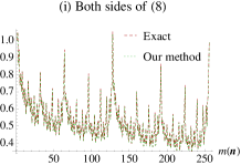
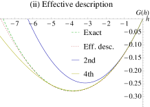
Figure 1: (color online) Statistical properties of current in an open boundary ASEP obtained by our computational method. We set $q=0.5$, $L=8$, $\alpha=0.8$, $\beta=0.8$, $\gamma=0.2$, and $\delta=0.2$. (i) We plot the right-hand side of (8) for $l=100$ and $\delta h=-0.02$ obtained from Monte Carlo simulations with (4) (Our method). We also plot the left-hand side of (8) obtained by the diagonalization of the matrix (6) for $l\delta h=-2$ (Exact). The $x$ axis represents $m({\boldsymbol{n}})=\sum_{i=0}^{L-1}n_{L-i}2^{i}$, which is the decimal value of the binary number ${\boldsymbol{n}}$. These two lines coincide with each other. (ii) $G(h)$ obtained from Monte Carlo simulations with the effective modified transition rate (9) (Eff. desc.). We also plot the largest eigenvalue of (6) with $h^{\prime}=0$ (Exact). Furthermore, we plot the truncated cumulant expansions up to the second order (2nd) and the fourth order (4th), which were calculated using the exact formula of ASEP Gorissen ; Gorissen2 .

Asymmetric simple exclusion process (ASEP).β€”As a demonstration of our method, we study the large deviation statistics of one-dimensional lattice gas models. We first consider a lattice of size $L$ with open boundary conditions, where each of the sites accommodates at most one particle. We denote a particle configuration by ${\boldsymbol{n}}\equiv(n_{i})_{i=1}^{L}$, where $n_{i}$ takes a value of $1$ (occupied) or 00 (empty). The transition rate $w({\boldsymbol{n}}\rightarrow{\boldsymbol{n}}^{\prime})$ is defined as follows. A particle moves to the left empty site with a rate $q$ and to the right empty site with a rate $1$. A particle is injected into the boundary site $i=1$ ($i=L$) at a rate $\alpha$ ($\delta$) and the particle at the boundary site $i=1$ ($i=L$) is removed at a rate $\gamma$ ($\beta$). This model is called ASEP. We focus on bulk current defined as $\alpha({\boldsymbol{n}}\rightarrow{\boldsymbol{n}}^{\prime})=1/(L-1)\sum_{i=1}^{L-1}j_{i}({\boldsymbol{n}}\rightarrow{\boldsymbol{n}}^{\prime})$, where $j_{i}({\boldsymbol{n}}\rightarrow{\boldsymbol{n}}^{\prime})$ takes the value of $1$ (or $-1$) when a particle moves from $i$ to $i+1$ ($i+1$ to $i$). By evaluating the transition rate (4) by Monte Carlo simulations and comparing it with the exact result obtained from the diagonalization of the matrix (6), we numerically confirm our formula (5). See Fig. 1 (i) for an example of the obtained results.

Next, we study an effective description of the exponential family. We introduce an effective transition rate $w_{\rm eff}^{h}$ with $L+1$ unknown parameters $(\psi_{h,i})_{i=0}^{L}$. Concretely, we define

$$w_{\rm eff}^{h}({\boldsymbol{n}}\rightarrow C_{i\rightarrow i\pm 1}{\boldsymbol{n}})\equiv w({\boldsymbol{n}}\rightarrow C_{i\rightarrow i\pm 1}{\boldsymbol{n}})e^{\pm h/(L-1)}\frac{\psi_{h,i\pm 1}}{\psi_{h,i}},$$ (9)

where $C_{i\rightarrow i\pm 1}$ denotes an operator that moves a particle from the site $i$ to the site $i\pm 1$. For the left (or right) boundary transition, we also define $w_{\rm eff}^{h}({\boldsymbol{n}}\rightarrow C_{\rm{L},\pm 1}{\boldsymbol{n}})\equiv w({\boldsymbol{n}}\rightarrow C_{\rm{L},\pm 1}{\boldsymbol{n}})(\psi_{h,1}/\psi_{h,0})^{\pm 1}$ (or $w_{\rm eff}^{h}({\boldsymbol{n}}\rightarrow C_{\rm{R},\pm 1}{\boldsymbol{n}})\equiv w({\boldsymbol{n}}\rightarrow C_{\rm{R},\pm 1}{\boldsymbol{n}})(\psi_{h,L}/\psi_{h,0})^{\pm 1}$), where $C_{{\rm L\ or\ R},a}$ denotes an operator that injects a particle into the boundary site (left or right) when $a=+1$ and removes a particle from the boundary site (left or right) when $a=-1$. The effective transition rate corresponds to an ASEP that has a new spatially varying transition rate. In other words, the effective transition rate is given by adding a one-body potential to the system.

The values of the parameters $(\psi_{h,i})_{i=0}^{L}$ are determined by our computational method. Let us suppose that we already have the values of the parameters $(\psi_{l\delta h,i})_{i=0}^{L}$. Then, we measure $\left\langle e^{\tau\delta hA(\omega)}\right\rangle_{{\boldsymbol{n}}}^{l\delta h}$ for $L+1$ different configurations ${\boldsymbol{n}}={\boldsymbol{n}}_{j}$ ($j=0,1,2,...,L)$. In particular, here, we set $({\boldsymbol{n}_{j}})_{i}=\delta_{ij}$ as the simplest choice. Next, by applying (4) to the effective transition rate (9), we obtain the following $L+1$ equations that connect the next parameters with the previous ones and the observed quantities: $\psi_{(l+1)\delta h,i}=\psi_{l\delta h,i}\left\langle e^{\tau\delta hA(\omega)}\right\rangle_{{\boldsymbol{n}}_{i}}^{l\delta h}$ ($i=0,1,2,...,L$). In this manner, the computation time becomes proportional to $O(L)$, which is substantially reduced from $O(2^{L})$.

By employing our computational method, we calculated $G(h)$, which is plotted in Fig. 1 (ii). In the same figure, for comparison, we also plot the exact result obtained from the eigenvalue problem of (6) and the truncated cumulant expansions up to the second and the fourth order obtained from the exact formula in Refs. Gorissen ; Gorissen2 . Although there is a small deviation between our result (red dotted line) and the exact result (green dashed line) around $h=-7$, the accuracy of our result is considerably better than the result for the truncated cumulant expansions (blue and yellow solid lines). This result indicates that rare fluctuations of the ASEP with this parameter set are well characterized by the effective transition rate (9). We expect that there exists a mathematical formula related to this observation. We remark that the variational expression proposed in BD ; BD2 can be derived from another variational principle provided in Refs. Discussion_of_modifiedTransitionrate ; Discussion_of_modifiedTransitionrate2 if we are allowed to use the effective transition rate (9) in the limit $L\rightarrow\infty$. We will study the effective transition rate (9) more systematically in future.

Refer to caption
Refer to caption
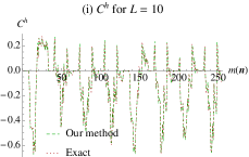
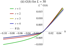
Figure 2: (color online) Statistical properties of an activity in a FA model for $c=0.3$. (i) For $L=10$ with $r=4$, we plot $C^{l\delta h}((n_{1+j})_{j=1}^{r})$ obtained from our method (Our method), where we set $l=40$ and $\delta h=-0.0025$. The $x$ axis represents $m({\boldsymbol{n}})=\sum_{i=0}^{r-1}n_{L-i}2^{i}+\sum_{i=r}^{2r-1}n_{2r+1-i}2^{i}$. On the same figure, we also plot $\phi^{l\delta h,0}(F_{1}{\boldsymbol{n}})/\phi^{l\delta h,0}({\boldsymbol{n}})$ with ${\boldsymbol{n}}=(0,n_{2},...,n_{r+1},0,...,0,n_{L-r+1},...n_{L})$ obtained from the diagonalization of the matrix (6) for $L=10$, $l\delta h=-0.1$ (Exact). These two lines coincide each other. (ii) $G(h)/L$ as a function of $h$ with the truncating number $r=1,2,3$, and $4$ for $L=30$. We also plot the result obtained from the population dynamics (P. D.) method Populationdynamics ; Populationdynamics2 as a black dashed line.

Fredrickson–Andersen (FA) model.β€”We next consider a FA model in a one-dimensional lattice of size $L$ with periodic boundary conditions. An occupation variable $n_{i}$, which takes a value of 0 (empty) or 1 (occupied), is defined for each site $i$. From a configuration ${\boldsymbol{n}}=(n_{i})_{i=1}^{L}$ to $F_{i}{\boldsymbol{n}}\equiv(n_{1},n_{2},...,1-n_{i},...,n_{L})$, a transition rate is defined as $w({\boldsymbol{n}}\rightarrow F_{i}{\boldsymbol{n}})\equiv[(1-c)n_{i}+c(1-n_{i})]f_{i}({\boldsymbol{n}})$, where the function $f_{i}({\boldsymbol{n}})\equiv n_{i-1}+n_{i+1}$ represents the kinetic constraints. Since the detailed balance condition is independent of $f_{i}({\boldsymbol{n}})$, the stationary probability $p({\boldsymbol{n}})$ is derived as $p({\boldsymbol{n}})=\prod_{i=1}^{L}[cn_{i}+(1-c)(1-n_{i})]$. Although the stationary state is trivial, the system exhibits a dynamical phase transition garrahan ; garrahan2 , which might be related to dynamical heterogeneities KCMReview1 ; KCMReview2 . In order to study the dynamical phase transition, we consider the large deviation statistics of the time-averaged value of an activity defined as $\alpha({\boldsymbol{n}}\rightarrow{\boldsymbol{n}}^{\prime})=1$. The dynamical phase transition has been determined as the singularity of the cumulant generating function in the limit $L\to\infty$ garrahan ; garrahan2 .

Here, we apply our method to this model. We define the effective transition rate as $w^{h}_{\rm eff}({\boldsymbol{n}}\rightarrow F_{i}{\boldsymbol{n}})\equiv w({\boldsymbol{n}}\rightarrow F_{i}{\boldsymbol{n}})e^{h}[C^{h}((n_{i\pm j})_{j=1}^{r})]^{1-2n_{i}}$, where $r$ is a truncating number of the interaction range and $C^{h}((n_{i\pm j})_{j=1}^{r})$ is an unknown function of local variables. We note that the transition rate improves in accuracy up to $r\simeq L/2$ as $r$ increases. For each $r$, in the same way as the application to the ASEP, $C^{h}((n_{1\pm j})_{j=1}^{r})$ is iteratively determined as $C^{(l+1)\delta h}((n_{1\pm j})_{j=1}^{r})=C^{l\delta h}((n_{1\pm j})_{j=1}^{r})\left\langle e^{\tau\delta hA(\omega)}\right\rangle_{F_{1}{\boldsymbol{n}}}^{l\delta h}/\left\langle e^{\tau\delta hA(\omega)}\right\rangle_{{\boldsymbol{n}}}^{l\delta h}$, where ${\boldsymbol{n}}=(0,n_{2},...,n_{r+1},0,...,0,n_{L-r+1},...n_{L})$. First, for small $L$, we check the validity of the obtained $C^{h}((n_{1\pm j})_{j=1}^{r})$ by comparing it with the result obtained from the diagonalization of the matrix (6). An example of the result is shown in Fig. 2 (i). Next, we fix relatively large $L$, and we obtain $G(h)$ for several values of $r$. We plot the obtained graph of $G(h)$ in Fig. 2 (ii). In the same figure, we also plot the result obtained by employing the population dynamics method Populationdynamics ; Populationdynamics2 . We observe that the curve for $r=4$ appears to be sufficient to explain the kinklike behavior of $G(h)$ near $h=0$. This result suggests that the long-range interactions for the modified transition rate $w^{h}_{\rm eff}({\boldsymbol{n}}\rightarrow{\boldsymbol{n}}^{\prime})$ may not be relevant to the dynamical phase transition observed in $G(h)$. The long-range nature of the effective interactions has also been studied very recently in Ref. JackRecent for the East model. In order to investigate the singular behavior of $G(h)$ in greater detail, a scaled biasing parameter $\tilde{h}\equiv hL$ has been used in this system bodineau1 ; bodineau2 . It has been mathematically proved that $\tilde{G}(\tilde{h})=G(\tilde{h}/L)$ is not an analytic function in the limit $L\to\infty$ bodineau1 ; however, the nature of the singularity has not thus far been elucidated. In suppl3 , we show that our method can also be applied to obtain the reliable $L$ dependence of $\tilde{G}(\tilde{h})$.

Conclusion.β€” In this Letter, we formulated the evolution rule (4) in an exponential family for large deviation statistics. By this method, rare events are identified as typical events in modified systems, which are continuously generated via an iterative measurement-and-feedback procedure. For spatially extended many-body systems, where the number of degrees of freedom increases as an exponential function of the system size, we also proposed a method for obtaining an effective description of the exponential family as a natural extension of our method. As examples of application of our method, we studied an ASEP and a FA model. By numerical experiments with our method, we observed that the exponential family of the ASEP was well described by another reparametrized ASEP, and that the kinklike behavior of $G(h)$ of the FA model near $h=0$ was shown in an effective description without long-range interactions. By performing further systematic numerical studies, we expect to obtain more quantitative information for large deviation statistics in spatially extended many-body systems. We believe that the formula (5) plays a fundamental role in large deviation theory, and, furthermore, we believe that our method provides a practically useful algorithm for numerical experiments of large deviation statistics.

T. N. thanks F. van Wijland and V. Lecomte for related discussions. This study was supported by Grant-in-Aid for JSPS Fellows No. 247538, KAKENHI No. 2234019, No. 25103002, and the JSPS Core-to-Core program β€œNonequilibrium Dynamics of Soft Matter and Information.”

References

  • (1) D. Frenkel and B. Smit, Understanding Molecular Simulation (Academic Press, San Diego, 2001).
  • (2) P. G. Bolhuis, D. Chandler, C. Dellago, and P. L. Geissler, Annu. Rev. Phys. Chem. 53, 291 (2002).
  • (3) T. S. van Erp, D. Moroni, and P. G. Bolhuis, J. Chem. Phys. 118, 7762 (2003).
  • (4) T. S. van Erp and P. G. Bolhuis, J. Comput. Phys. 205, 157 (2005).
  • (5) R. J. Allen, P. B. Warren, and P. R. ten Wolde, Phys. Rev. Lett. 94, 018104 (2005).
  • (6) R. J. Allen, D. Frenkel, and P. R. ten Wolde, J. Chem. Phys. 124, 024102 (2006).
  • (7) C. Giardina, J. Kurchan, and L. Peliti, Phys. Rev. Lett. 96, 120603 (2006).
  • (8) C. Giardina, J. Kurchan, V. Lecomte and J. Tailleur, J. Stat. Phys. 145, 787 (2011).
  • (9) A. Dembo and O. Zeitouni, Large deviations techniques and applications (Springer, New York, 1998).
  • (10) H. Touchette, Phys. Rep. 478, 1, (2009).
  • (11) D. J. Evans, E. G. D. Cohen, and G. P. Morriss, Phys. Rev. Lett. 71, 2401 (1993).
  • (12) J. L. Lebowitz and H. Spohn, J. Stat. Phys. 95, 333 (1999).
  • (13) T. Bodineau and B. Derrida, Phys. Rev. Lett. 92, 180601 (2004).
  • (14) T. Bodineau and B. Derrida, J. Stat. Phys. 123, 277 (2006).
  • (15) J. P. Garrahan, R. L. Jack, V. Lecomte, E. Pitard, K. van Duijvendijk, and F. van Wijland, Phys. Rev. Lett. 98, 195702 (2007).
  • (16) J. P. Garrahan, R. L. Jack, V. Lecomte, E. Pitard, K. van Duijvendijk, and F. van Wijland, J. Phys. A 42, 075007 (2009).
  • (17) C. Maes, K. NetočnΓ½, and B. Wynants, Phys. Rev. Lett. 107, 010601 (2011).
  • (18) A. Lazarescu and K. Mallick, J. Phys. A 44 315001 (2011).
  • (19) M. Gorissen, A. Lazarescu, K. Mallick, and C. Vanderzande, Phys. Rev. Lett. 109, 170601 (2012).
  • (20) R. M. L. Evans, Phys. Rev. Lett. 92, 150601 (2004).
  • (21) R. L. Jack and P. Sollich, Prog. Theor. Phys. Suppl. 184, 304 (2010).
  • (22) T. Nemoto and S.-i. Sasa, Phys. Rev. E 84, 061113 (2011).
  • (23) R. Chetrite and H. Touchette, Phys. Rev. Lett. 111, 120601 (2013).
  • (24) See Supplemental Material at [URL will be inserted by publisher] for the details of the derivation of (5).
  • (25) Y. Oono, The Nonlinear World: Conceptual Analysis and Phenomenology (Springer, New York, 2012).
  • (26) S. Sasa, Phys. Scr. 86, 058514 (2012).
  • (27) J. P. Garrahan, P. Sollich, and C. Toninelli, in Dynamical Heterogeneities in Glasses, Colloids, and Granular Media, edited by L. Berthier, G. Biroli, J.-P. Bouchaud, L. Cipelletti, and W. van Saarloos (Oxford University Press, Oxford, 2011).
  • (28) F. Ritort and P. Sollich, Adv. Phys. 52, 219 (2003).
  • (29) R. L. Jack and P. Sollich, J. Phys. A 47, 015003 (2014).
  • (30) T. Bodineau and C. Toninelli, Commun. Math. Phys. 311, 357 (2012).
  • (31) T. Bodineau, V. Lecomte, and C. Toninelli, J. Stat. Phys. 147, 1 (2012).
  • (32) See Supplemental Material at [URL will be inserted by publisher] for the application to obtain the reliable $L$ dependence of $\tilde{G}(\tilde{h})$.

Supplemental material for β€œComputation of large deviation statistics via iterative measurement-and-feedback procedure”

1. Derivation of the theoretical basis (5) in the text:

Here, we derive (5) in the text. As a preliminary, we consider a matrix

$$L^{h,0}_{{\boldsymbol{n}},{\boldsymbol{n}}^{\prime}}\equiv w({\boldsymbol{n}}^{\prime}\rightarrow{\boldsymbol{n}})e^{h\alpha({\boldsymbol{n}}^{\prime}\rightarrow{\boldsymbol{n}})}-\lambda({\boldsymbol{n}})\delta_{{\boldsymbol{n}},{\boldsymbol{n}}^{\prime}}.$$ (10)

Let $\phi^{h,0}$ and $G^{h,0}$ be the left eigenvector and the eigenvalue of the largest eigenvalue problem of (10). Then, we define a modified transition rate as

$$u^{h}({\boldsymbol{n}}^{\prime}\rightarrow{\boldsymbol{n}})\equiv w({\boldsymbol{n}}^{\prime}\rightarrow{\boldsymbol{n}})e^{h\alpha({\boldsymbol{n}}^{\prime}\rightarrow{\boldsymbol{n}})}\phi^{h,0}({\boldsymbol{n}})/\phi^{h,0}({\boldsymbol{n}}^{\prime}).$$ (11)

The path probability density in the steady state generated by $u^{h}$ is connected with the exponential family. We denote by $\left\langle f(\omega)\right\rangle^{u^{h}}$ the expected value of a time-extensive quantity $f(\omega)$ with respect to the path probability density. Then, it has been known that

$$\left\langle f(\omega)\right\rangle^{u^{h}}\simeq\frac{\left\langle f(\omega)e^{h\tau A(\omega)}\right\rangle}{\left\langle e^{h\tau A(\omega)}\right\rangle}.$$ (12)

See Ref. JackSollich_Suppl for the details of the derivation. This relation has been re-invented and used in many works, for example, in Refs. JackSollich_Suppl ; Discussion_of_modifiedTransitionrate_Suppl ; Chetrite_Touchette_Suppl . With the aid of (12), the relation (5) in the text may be derived from the equivalence between the transition rate $u^{h}$ and the transition rate $w^{h}$ introduced in the text.

In order to show the equivalence, we first consider the matrix defined by $u^{h}$:

$$L^{h,h^{\prime}}_{{\boldsymbol{n}},{\boldsymbol{n}}^{\prime}}\equiv u^{h^{\prime}}({\boldsymbol{n}}^{\prime}\rightarrow{\boldsymbol{n}})e^{h\alpha({\boldsymbol{n}}^{\prime}\rightarrow{\boldsymbol{n}})}-\lambda^{u^{h^{\prime}}}({\boldsymbol{n}})\delta_{{\boldsymbol{n}},{\boldsymbol{n}}^{\prime}}$$ (13)

with $\lambda^{u^{h^{\prime}}}({\boldsymbol{n}})\equiv\sum_{{\boldsymbol{n}}^{\prime}}u^{h}({\boldsymbol{n}}\rightarrow{\boldsymbol{n}}^{\prime})$. We denote the left eigenvector and the eigenvalue of the largest eigenvalue problem of (13) by $\phi^{h,h^{\prime}}$ and $G^{h,h^{\prime}}$. We then present the multiplicative property for the eigenvector and the additive property for the eigenvalue of the largest eigenvalue problem of (13), which are

$$\phi^{h+h^{\prime},0}=\phi^{h,h^{\prime}}\phi^{h^{\prime},0}$$ (14)

and

$$G^{h+h^{\prime},0}=G^{h,h^{\prime}}+G^{h^{\prime},0}.$$ (15)

The proof is the following. First, we write the eigenvalue equations for $\phi^{h+h^{\prime},0}$, $\phi^{h^{\prime},0}$, and $\phi^{h,h^{\prime}}$ as

$$\sum_{{\boldsymbol{n}}^{\prime}}w({\boldsymbol{n}}\rightarrow{\boldsymbol{n}}^{\prime})e^{(h+h^{\prime})\alpha({\boldsymbol{n}}\rightarrow{\boldsymbol{n}}^{\prime})}\frac{\phi^{h+h^{\prime},0}({\boldsymbol{n}}^{\prime})}{\phi^{h+h^{\prime},0}({\boldsymbol{n}})}-\lambda({\boldsymbol{n}})=G^{h+h^{\prime},0},$$ (16)
$$\sum_{{\boldsymbol{n}}^{\prime}}w({\boldsymbol{n}}\rightarrow{\boldsymbol{n}}^{\prime})e^{h^{\prime}\alpha({\boldsymbol{n}}\rightarrow{\boldsymbol{n}}^{\prime})}\frac{\phi^{h^{\prime},0}({\boldsymbol{n}}^{\prime})}{\phi^{h^{\prime},0}({\boldsymbol{n}})}-\lambda({\boldsymbol{n}})=G^{h^{\prime},0},$$ (17)

and

$$\begin{split}&\sum_{{\boldsymbol{n}}^{\prime}}w({\boldsymbol{n}}\rightarrow{\boldsymbol{n}}^{\prime})e^{(h+h^{\prime})\alpha({\boldsymbol{n}}\rightarrow{\boldsymbol{n}}^{\prime})}\frac{\phi^{h,h^{\prime}}({\boldsymbol{n}}^{\prime})\phi^{h^{\prime},0}({\boldsymbol{n}}^{\prime})}{\phi^{h,h^{\prime}}({\boldsymbol{n}})\phi^{h^{\prime},0}({\boldsymbol{n}})}-\lambda^{u^{h^{\prime}}}({\boldsymbol{n}})\\ &=G^{h,h^{\prime}}.\end{split}$$ (18)

Since the first term of (17) is equal to the second term of (18), these terms cancel each other when we sum (17) and (18). We thus obtain

$$\begin{split}&\sum_{{\boldsymbol{n}}^{\prime}}w({\boldsymbol{n}}\rightarrow{\boldsymbol{n}}^{\prime})e^{(h+h^{\prime})\alpha({\boldsymbol{n}}\rightarrow{\boldsymbol{n}}^{\prime})}\frac{\phi^{h,h^{\prime}}({\boldsymbol{n}}^{\prime})\phi^{h^{\prime},0}({\boldsymbol{n}}^{\prime})}{\phi^{h,h^{\prime}}({\boldsymbol{n}})\phi^{h^{\prime},0}({\boldsymbol{n}})}-\lambda({\boldsymbol{n}})\\ &=G^{h,h^{\prime}}+G^{h^{\prime},0}.\end{split}$$ (19)

From the Perron-Frobenius theory for irreducible matrices Seneta_Suppl , the positive eigenvector of $L_{{\boldsymbol{n}},{\boldsymbol{n}}^{\prime}}^{h,0}$ is unique. Thus, by comparing (16) with (19), we arrive at (14) and (15).

Second, we show a relation between the eigenvector $\phi^{h,h^{\prime}}$ and $\left\langle e^{\tau hA(\omega)}\right\rangle_{{\boldsymbol{n}}}$. We start with the time-evolution equation of $\left\langle e^{h\tau A(\omega)}\delta_{{\boldsymbol{n}}(\tau),{\boldsymbol{n}}}\right\rangle_{{\boldsymbol{n}}_{0}}$,

$$\frac{\partial\left\langle e^{h\tau A(\omega)}\delta_{{\boldsymbol{n}}(\tau),{\boldsymbol{n}}}\right\rangle_{{\boldsymbol{n}}_{0}}}{\partial\tau}=\sum_{{\boldsymbol{n}}^{\prime}}L_{{\boldsymbol{n}},{\boldsymbol{n}}^{\prime}}^{h,0}\left\langle e^{h\tau A(\omega)}\delta_{{\boldsymbol{n}}(\tau),{\boldsymbol{n}}^{\prime}}\right\rangle_{{\boldsymbol{n}}_{0}}.$$ (20)

See Ref. garrahan2_Suppl for the derivation. We can rewrite this expression as

$$\frac{\partial\left\langle e^{h\tau A(\omega)}\right\rangle_{{\boldsymbol{n}}}}{\partial\tau}=\sum_{{\boldsymbol{n}}^{\prime}}L_{{\boldsymbol{n}}^{\prime},{\boldsymbol{n}}}^{h,0}\left\langle e^{h\tau A(\omega)}\right\rangle_{{\boldsymbol{n}}^{\prime}}.$$ (21)

This time evolution equation indicates an asymptotic expression

$$\phi^{h,0}({\boldsymbol{n}})\simeq\left\langle e^{\tau hA(\omega)}\right\rangle_{{\boldsymbol{n}}}.$$ (22)

We note that the same method may be applied to the system with $u^{h}$. In this case, the matrix appeared in (20) is replaced by $L^{h,h^{\prime}}_{{\boldsymbol{n}},{\boldsymbol{n}}^{\prime}}$, which leads to

$$\phi^{h,h^{\prime}}({\boldsymbol{n}})\simeq\left\langle e^{\tau hA(\omega)}\right\rangle_{{\boldsymbol{n}}}^{u^{h^{\prime}}}.$$ (23)

Finally, from the results above, we show the equivalence between $w^{h}$ and $u^{h}$. We fix an increment $\delta h$. First, $w^{\delta h}$ is defined as

$$w^{\delta h}({\boldsymbol{n}}\rightarrow{\boldsymbol{n}}^{\prime})=w({\boldsymbol{n}}\rightarrow{\boldsymbol{n}}^{\prime})e^{\delta h\alpha({\boldsymbol{n}}\rightarrow{\boldsymbol{n}}^{\prime})}\frac{\left\langle e^{\tau\delta hA(\omega)}\right\rangle_{{\boldsymbol{n}}^{\prime}}}{\left\langle e^{\tau\delta hA(\omega)}\right\rangle_{{\boldsymbol{n}}}}.$$ (24)

With the relation (22), the definition leads to

$$w^{\delta h}\simeq u^{\delta h}.$$ (25)

The next transition rate $w^{2\delta h}$ is defined as

$$\begin{split}&w^{2\delta h}({\boldsymbol{n}}\rightarrow{\boldsymbol{n}}^{\prime})=w^{\delta h}({\boldsymbol{n}}\rightarrow{\boldsymbol{n}}^{\prime})e^{\delta h\alpha({\boldsymbol{n}}\rightarrow{\boldsymbol{n}}^{\prime})}\frac{\left\langle e^{\tau\delta hA(\omega)}\right\rangle_{{\boldsymbol{n}}^{\prime}}^{\delta h}}{\left\langle e^{\tau\delta hA(\omega)}\right\rangle_{{\boldsymbol{n}}}^{\delta h}},\end{split}$$ (26)

where $\left\langle\ \right\rangle_{{\boldsymbol{n}}}^{\delta h}$ is the expected value in the modified system, which is equivalent to $\left\langle\ \right\rangle_{{\boldsymbol{n}}}^{u^{\delta h}}$ due to (25). Then, from the multiplicative property (14) with (23), we obtain

$$w^{2\delta h}\simeq u^{2\delta h}.$$ (27)

By iterating this procedure, we thus arrive at the equivalence between $u^{h}$ and $w^{h}$. That is, a set of transition rates

$$\begin{split}&w^{l\delta h}({\boldsymbol{n}}\rightarrow{\boldsymbol{n}}^{\prime})=w({\boldsymbol{n}}\rightarrow{\boldsymbol{n}}^{\prime})e^{l\delta h\alpha({\boldsymbol{n}}\rightarrow{\boldsymbol{n}}^{\prime})}\prod_{k=0}^{l-1}\frac{\left\langle e^{\tau\delta hA(\omega)}\right\rangle_{{\boldsymbol{n}}^{\prime}}^{k\delta h}}{\left\langle e^{\tau\delta hA(\omega)}\right\rangle_{{\boldsymbol{n}}}^{k\delta h}}\end{split}$$ (28)

with $l=0,1,2,...$ satisfies

$$w^{l\delta h}\simeq u^{l\delta h}$$ (29)

for $l=0,1,2,...$.

2. Scaled cumulant generating function for a FA model:

(i). Scaled cumulant generating function and obtained result:

In order to investigate the singular behavior of $G(h)$ in greater detail, a scaled biasing parameter $\tilde{h}\equiv hL$ has been used in one-dimensional FA model bodineau1_Suppl ; bodineau2_Suppl . It has been mathematically proved that $\tilde{G}(\tilde{h})=G(\tilde{h}/L)$ is not an analytic function in the limit $L\to\infty$ bodineau1_Suppl ; however, the nature of the singularity has not thus far been elucidated. The problem has been numerically studied by employing the population dynamics method bodineau2_Suppl . However, it seems that the result does not exhibit good convergence of $\tilde{G}(\tilde{h})$ for relatively large values of $L$. In this supplemental material, we show that our method can be applied to obtain the reliable $L$ dependence of $\tilde{G}(\tilde{h})$ up to $L=60$.

In the text, for the one-dimensional FA model, we introduced the effective transition rate defined as

$$\begin{split}w^{h}_{\rm eff}({\boldsymbol{n}}\rightarrow F_{i}{\boldsymbol{n}})\equiv w({\boldsymbol{n}}\rightarrow F_{i}{\boldsymbol{n}})e^{h}\left[C^{h}((n_{i\pm j})_{j=1}^{r})\right]^{1-2n_{i}},\end{split}$$ (30)

where $C^{h}((n_{i\pm j})_{j=1}^{r})$ was an unknown function of local variables characterized by the truncating number $r$. By investigating $\tilde{G}(\tilde{h})$ via the effective description with several truncating numbers $r$ and system sizes $L$, we will judge that the result with $r=4$ is sufficiently accurate to obtain the true $L$-dependence of $\tilde{G}(\tilde{h})$. We present this argument in the next section. Here, we show the obtained $L$ dependence of $\tilde{G}(\tilde{h})$. We plot $\tilde{G}(\tilde{h})$ with $r=4$ fixed for various values of $L$ in Fig. 3. Although it has been conjectured that $\tilde{G}(\tilde{h})$ contains a non-differentiable point in the limit $L\to\infty$ bodineau1_Suppl , our result does not show any clear sign of such a point in $\tilde{G}(\tilde{h})$ up to $L=60$.

Refer to caption
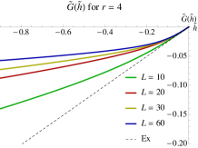
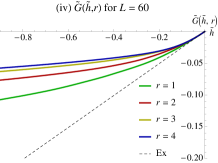
Figure 3: (Color online) Cumulant generating functions obtained from our computational method for a FA model with $c=0.3$. We plot $\tilde{G}(\tilde{h})\equiv G(\tilde{h}/L)$ for various values of $L$ with $r=4$ fixed. We also plot the straight line (Ex) of the slope $4c^{2}(1-c)$, which is the expected value of the activity in the original system with $h=0$.

(ii). Truncating number of a FA model:

In this section, we present the evidence that $r=4$ is sufficiently large to describe the true $L$-dependence of the scaled function $\tilde{G}(\tilde{h})\equiv G(L^{-1}\tilde{h})$.

Refer to caption
Refer to caption
Refer to caption
Refer to caption
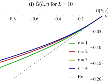
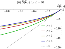
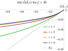
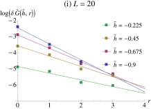
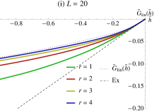
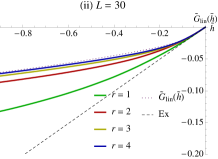
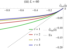
Figure 4: (Color online) $\tilde{G}(\tilde{h},r)$ for $r=1,2,3$, and $4$ with $L=10$ (i), 20 (ii), 30 (iii), and 60 (iv). We set $c=0.3$. We also plot the straight line (Ex) with the slope $4c^{2}(1-c)$ in each figure.

First, we denote by $\tilde{G}(\tilde{h},r)$ our calculation result of $\tilde{G}(\tilde{h})$ obtained with truncating number $r$. In Fig. 4, we show $\tilde{G}(\tilde{h},1)$, $\tilde{G}(\tilde{h},2)$, $\tilde{G}(\tilde{h},3)$, and $\tilde{G}(\tilde{h},4)$ for $L=10$ (i), $20$ (ii), $30$ (iii), and $60$ (iv). We also plot the straight line (Ex) with the slope $4c^{2}(1-c)$ in each figure, which is the expected value of the activity in the original system with $\tilde{h}=0$. This straight line is equivalent to $\tilde{G}(\tilde{h},0)$, since there are no modifications for $r=0$. In Fig. 4, we observe that the differences between $\tilde{G}(\tilde{h})$ with $r=3$ and that with $r=4$ are small even for larger $L$ (say $L=20,30$, and $60$).

Refer to caption
Refer to caption
Refer to caption
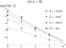
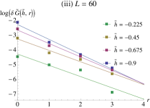
Figure 5: (Color online) The logarithm of the difference function $\delta\tilde{G}(\tilde{h},r)$ for $r=0,1,2$, and $3$ with $L=20$ (i), 30 (ii), and 60 (iii). We set $c=0.3$.

We then quantify these small differences by introducing a difference function

$$\delta\tilde{G}(\tilde{h},r)=\tilde{G}(\tilde{h},r+1)-\tilde{G}(\tilde{h},r).$$ (31)

In Fig. 5, we plot the logarithm of $\delta G(r,h)$ as a function of $r$ for $\tilde{h}=-0.225,-0.45,-0.675$ and $-0.9$ with $L=20$ (i), $30$ (ii), and $60$ (iii). In the same figure, we also plot straight lines, which were obtained from a least squares fit of the data points. We observe that the decay of $\delta\tilde{G}$ with increasing $\tilde{r}$ is exponentially fast (or faster than exponential decay). We thus expect that larger $r$ is not needed to obtain the correct $\tilde{G}(\tilde{h})$.

Refer to caption
Refer to caption
Refer to caption
Figure 6: (Color online) $\tilde{G}(\tilde{h},r)$ and $\tilde{G}_{\rm lin}(\tilde{h})$ for $r=1,2,3,$ and $4$ with $L=20$ (i), 30 (ii), and 60 (iii). We set $c=0.3$.

Finally, by assuming the shape of $\delta\tilde{G}(\tilde{h},r)$ as an exponentially decaying function, we estimate possible errors due to the truncation of $r$ with $r=4$. Inspired by the result of Fig. 5, we define

$$\delta\tilde{G}_{\rm lin}(\tilde{h},r)=e^{a(\tilde{h})r+b(\tilde{h})},$$ (32)

where $a(\tilde{h})r+b(\tilde{h})$ is a linear function of $r$, which is determined from the least squares fit of data points $\log\delta\tilde{G}(\tilde{h},r=0)$, $\log\delta\tilde{G}(\tilde{h},r=1)$, $\log\delta\tilde{G}(\tilde{h},r=2)$, and $\log\delta\tilde{G}(\tilde{h},r=3)$. The examples of the linear function are solid lines in Fig. 5. Then, by using $\delta\tilde{G}_{\rm lin}$, we define an interpolation function $\tilde{G}_{\rm lin}(\tilde{h},r)$ of $\tilde{G}(\tilde{h},r)$ for larger $r$ as

G~lin​(h~,r)≑G~​(h~,4)+βˆ‘s=4rβˆ’1δ​G~lin​(h~,s)subscript~𝐺lin~β„Žπ‘Ÿ~𝐺~β„Ž4superscriptsubscript𝑠4π‘Ÿ1𝛿subscript~𝐺lin~β„Žπ‘ \tilde{G}_{\rm lin}(\tilde{h},r)\equiv\tilde{G}(\tilde{h},4)+\sum_{s=4}^{r-1}\delta\tilde{G}_{\rm lin}(\tilde{h},s) (33)

for $r=5,6,...$. Since $\tilde{G}(\tilde{h},r)$ with $r\simeq L/2$ is equal to $\tilde{G}(\tilde{h})$, we thus define an interpolation function of $\tilde{G}(\tilde{h})$ as

$$\tilde{G}_{\rm lin}(\tilde{h})\equiv\tilde{G}_{\rm lin}(\tilde{h},L/2-1).$$ (34)

We plot $\tilde{G}_{\rm lin}(\tilde{h})$ with $\tilde{G}(\tilde{h},r)$ for $r=1,2,3$, and 4 in Fig. 6. In the figure, the differences between $\tilde{G}_{\rm lin}(\tilde{h})$ and $\tilde{G}(\tilde{h},4)$ are quite small, so that we judge that $r=4$ is sufficiently large to describe the true $L$-dependence of $\tilde{G}(\tilde{h})$.

References

  • (1) R. L. Jack and P. Sollich, Prog. Theor. Phys. Suppl. 184, 304 (2010).
  • (2) T. Nemoto and S.-i. Sasa, Phys. Rev. E 84, 061113 (2011).
  • (3) R. Chetrite and H. Touchette, Phys. Rev. Lett. 111, 120601 (2013).
  • (4) E. Seneta, Non-Negative Matrices and Markov Chains, 2nd ed. (Springer, New York, 2006).
  • (5) J. P. Garrahan, R. L. Jack, V. Lecomte, E. Pitard, K. van Duijvendijk, and F. van Wijland, J. Phys. A 42, 075007 (2009).
  • (6) T. Bodineau and C. Toninelli, Commun. Math. Phys. 311, 357 (2012).
  • (7) T. Bodineau, V. Lecomte, and C. Toninelli, J. Stat. Phys. 147, 1 (2012).