Inflation, Leptogenesis, and Yukawa Quasi-Unification
within a Supersymmetric Left-Right Model

Abstract

A simple extension of the minimal left-right symmetric supersymmetric grand unified theory model is constructed by adding two pairs of superfields. This naturally violates the partial Yukawa unification predicted by the minimal model. After including supergravity corrections, we find that this extended model naturally supports hilltop F-term hybrid inflation along its trivial inflationary path with only a very mild tuning of the initial conditions. With a convenient choice of signs of the terms in the Kähler potential, we can reconcile the inflationary scale with the supersymmetric grand unified theory scale. All the current data on the inflationary observables are readily reproduced. Inflation is followed by non-thermal leptogenesis via the decay of the right-handed neutrinos emerging from the decay of the inflaton and any possible washout of the lepton asymmetry is avoided thanks to the violation of partial Yukawa unification. The extra superfields also assist us in reducing the reheat temperature so as to satisfy the gravitino constraint. The observed baryon asymmetry of the universe is naturally reproduced consistently with the neutrino oscillation parameters.

I Introduction

One of the most natural and well-motivated inflation models is, certainly, the supersymmetric (SUSY) F-term hybrid inflation (FHI) hybrid ; susyhybrid . It is realized at (or close to) the SUSY grand unified theory (GUT) scale $M_{\rm GUT}\simeq 2.86\times 10^{16}~{}{\rm GeV}$ and can be easily linked to extensions lectures of the minimal supersymmetric standard model (MSSM) which provide solutions to a number of problems of the MSSM. Namely, the $\mu$-problem of MSSM can be solved via a direct coupling of the inflaton to the electroweak Higgs doublet superfields dvali or via a Peccei-Quinn (PQ) symmetry rsym ; pqhi , which also solves pq the strong CP problem. Also, baryon-number conservation can be an automatic consequence dvali of a R symmetry and the baryon asymmetry of the universe (BAU) can be generated via non-thermal leptogenesis ntlepto , which takes place through the out-of-equilibrium decay of the decay products of the inflaton.

Trying to embed SUSY FHI into a concrete SUSY GUT model, we face the following challenges: (i) the possible production of topological defects kibble ; monopole during the GUT phase transition at the end of FHI, which in the case of magnetic monopoles or domain walls is cosmologically disastrous, (ii) the mismatch hinova between the inflationary scale and the SUSY GUT scale, and (iii) the possible washout of the generated lepton-number asymmetry due to the smallness of the lightest right-handed neutrino mass dictated by the various types of Yukawa unification (YU) conditions predicted by some GUT models.

Here we present a model based on the left-right symmetric GUT gauge group $G_{\rm LR}={\rm SU(3)_{c}}\times{\rm SU(2)_{L}}\times{\rm SU(2)_{R}}\times{\rm U(1)}_{B-L}$, which aims to surpass the problems mentioned above. Namely, $G_{\rm LR}$ does not lead to production of magnetic monopoles as higher gauge groups, such as the Pati-Salam group, do. Moreover, invoking higher order terms in the Kähler potential with a suitable arrangement of their signs, as done in Ref. rlarge , we succeed to overcome the second of the aforementioned difficulties of SUSY FHI. It is important to note that the same form of the Kähler potential has been proposed in order to reconcile the value of the scalar spectral index $n_{\rm s}$ obtained within SUSY FHI with the present data wmap ; plin .

Finally and probably most importantly, the problem (iii) is overcome by conveniently extending the superfield content of the simplest – see e.g. Ref. vlachos – GUT model based on $G_{\rm LR}$. Namely, we introduce a pair of ${\rm SU(2)_{L}}\times{\rm SU(2)_{R}}$ bidoublet superfields and a pair of ${\rm SU(2)_{\rm R}}$ triplet superfields, which lead to a sizable violation of the neutrino-$\tau$ (and top-bottom) YU predicted by the simplest model. As a consequence, the lightest right-handed neutrino mass, which depends heavily on the lightest neutrino Dirac mass, may become large enough so that any washout of the pre-generated lepton asymmetry is elegantly evaded. Moreover, the ${\rm SU(2)_{\rm R}}$ triplet superfields enter the inflationary sector of the model leading to a variety of possible inflationary scenarios – see Refs. nshift ; nsmooth ; ax2 ; ax3 – as well as to extra contributions to the radiative corrections on the inflationary paths used in these scenarios. Here we choose to analyze FHI along the trivial inflationary trajectory of this model. We should note that these same triplet superfields assist us to reduce the predicted reheat temperature to an acceptable level.

Imposing, in addition, a number of theoretical and observational constraints originating from the data on the inflationary observables, the boundedness below of the inflationary potential, the observed BAU, the gravitino constraint gravitino ; kohri , and the data on the neutrino oscillation parameters, we find a wide and natural allowed space of parameters. The resulting FHI inflationary scenario is of the hilltop type lofti requiring a mild tuning of the initial conditions gpp to yield acceptable values of the scalar spectral index and a rather large value of the gravitino mass to fulfill the gravitino constraint.

In Sec. II, we present the basic ingredients of our model, while, in Sec. III, we describe the inflationary scenario. We then discuss the inflationary requirements and their implications for the model parameters in Sec. IV. Our next step is to outline the mechanism of non-thermal leptogenesis in Sec. V and update the constraints on the model parameters taking into account the post-inflationary requirements in Sec. VI. We summarize our conclusions in Sec. VII. Finally, in Appendix A, we present a numerical analysis of the reheating process in our model.

II The SUSY Left-Right Symmetric Model

We will outline the salient features of our model in Sec. II.1 and analyze the various parts of its superpotential in Sec. II.2. Finally, in Sec. II.3, we will derive a set of Yukawa quasi-unification conditions which play a key role in our model.

II.1 Superfield Content and Symmetries

As already mentioned, we adopt the left-right symmetric gauge group $G_{\rm LR}={\rm SU(3)_{c}}\times{\rm SU(2)_{L}}\times{\rm SU(2)_{R}}\times{\rm U(1)}_{B-L}$. This gauge group is broken down to the standard model (SM) gauge group $G_{\rm SM}$ at a scale close to the SUSY GUT scale $M_{\rm GUT}$ through the vacuum expectation values (VEVs) acquired by a conjugate pair of ${\rm SU}(2)_{\rm R}$ doublet left-handed Higgs superfields $\Phi$ and $\bar{\Phi}$ with $B-L=1,~{}-1$ respectively. In this model, no magnetic monopoles monopole or cosmic strings kibble are produced trotta at the end of inflation and, therefore, we are not obliged to modify smooth ; shifted the standard realization of SUSY FHI to avoid monopole production, or impose extra restrictions on the parameters – as e.g. in Ref. mairi .

The representations and transformations under $G_{\rm LR}$ of the various matter and Higgs superfields of the model are presented in Table 1 ($U_{\rm c}\in{\rm SU(3)_{c}}$, $U_{\rm L}\in{\rm SU(2)_{L}}$, $U_{\rm R}\in{\rm SU(2)_{R}}$ and T, $\dagger$, and $\ast$ stand for the transpose, the Hermitian conjugate (H.c.), and the complex conjugate of a matrix respectively). The model also possesses three global ${\rm U(1)}$ symmetries, namely a R symmetry, a PQ symmetry, and the baryon-number ($B$) symmetry. The corresponding charges are shown in Table 1 too. Note, in passing, that such continuous global symmetries can effectively arise laz1 from the discrete symmetries emerging in many compactified string theories (see e.g. Ref. laz2 ).

Table 1: The superfield content of the model.

Super-	Represen-	Transfor-	Global
fields	tations	mations	Symmetries
	under $G_{\rm LR}$	under $G_{\rm LR}$	$R$	$PQ$	$B$
Matter Fields
$l_{i}$	$({\bf 1,2,1},-1)$	$l_{i}U_{\rm L}^{\dagger}$	$1$	$-1$	$0$
$l^{c}_{i}$	$({\bf 1,1,2},1)$	$U_{\rm R}^{\ast}l^{c}_{i}$	$1$	$0$	$0$
$q_{i}$	$({\bf 3,2,1},1/3)$	$q_{i}U_{\rm L}^{\dagger}\ U_{\rm c}^{\mbox{\sf\scriptsize T}}$	$1$	$-1$	$1/3$
$q^{c}_{i}$	$({\bf\bar{3},1,2},-1/3)$	$U_{\rm c}^{\ast}\ U_{\rm R}^{\ast}q^{c}_{i}$	$1$	$0$	$-1/3$
Higgs Fields
$\Phi$	$({\bf 1,1,2},1)$	$U_{\rm R}^{\ast}\Phi$	$0$	$0$	$0$
$\bar{\Phi}$	$({\bf 1,1,2},-1)$	$\bar{\Phi}U^{\mbox{\sf\scriptsize T}}_{\rm R}$	$0$	$0$	$0$
$S$	$({\bf 1,1,1},0)$	$S$	$2$	$0$	$0$
${I{\kern-2.6pth}}$	$({\bf 1,2,2},0)$	$U_{\rm L}{I{\kern-2.6pth}}U^{\mbox{\sf\scriptsize T}}_{\rm R}$	$0$	$1$	$0$
$N$	$({\bf 1,1,1},0)$	$N$	$1$	$-1$	$0$
$\bar{N}$	$({\bf 1,1,1},0)$	$\bar{N}$	$0$	$1$	$0$
Extra Higgs Fields
${I{\kern-2.6pth}}^{\prime}$	$({\bf 1,2,2},0)$	$U_{\rm L}{I{\kern-2.6pth}}^{\prime}U^{\mbox{\sf\scriptsize T}}_{\rm R}$	$0$	$1$	$0$
${\bar{I{\kern-2.6pth}}}^{\prime}$	$({\bf 1,2,2},0)$	$U_{\rm L}{\bar{I{\kern-2.6pth}}}^{\prime}U^{\mbox{\sf\scriptsize T}}_{\rm R}$	$2$	$-1$	$0$
$T$	$({\bf 1,1,3},0)$	$U_{\rm R}TU_{\rm R}^{\dagger}$	$0$	$0$	$0$
$\bar{T}$	$({\bf 1,1,3},0)$	$U_{\rm R}\bar{T}U_{\rm R}^{\dagger}$	$2$	$0$	$0$

The lepton and quark superfields are $l_{i}$, $l^{c}_{i}$ and $q_{i}$, $q^{c}_{i}$ ($i=1,2,3$) respectively – we follow here the same representation of the superfields under ${\rm SU(2)_{L}}\times{\rm SU(2)_{R}}$ as in Ref. klpnova . In the simplest version of the model without the extra Higgs superfields in Table 1, the electroweak Higgs doublets $H_{1}$ and $H_{2}$ which couple to the down- and up-type quarks respectively belong to the bidoublet superfield ${I{\kern-2.6pth}}$. So, as one can easily see, all the requirements pana for partial YU, i.e. the ‘asymptotic’ (at $M_{\rm GUT}$) equality of the Yukawa coupling constants of the $t$- and the $b$-quark as well as of the $\tau$-neutrino $\nu_{\tau}$ and the $\tau$-lepton $\tau$, are fulfilled. As already indicated, the breaking of $G_{\rm LR}$ down to $G_{\rm SM}$ is achieved by the superheavy VEVs ($\sim M_{\rm GUT}$) of the conjugate pair of Higgs superfields $\Phi$, $\bar{\Phi}$ along their right-handed neutrino type components ($\nu^{c}_{\Phi}$, $\bar{\nu}^{c}_{\Phi}$). The model also contains a gauge singlet $S$, which triggers the breaking of $G_{\rm LR}$ and a pair of gauge singlets $N$, $\bar{N}$ for solving rsym the $\mu$ problem of the MSSM via the PQ symmetry.

The partial YU between the $b$- and the $t$-quark implied by the simplest left-right symmetric model is not compatible gYqu ; klpnova ; Antuch with the constrained MSSM (CMSSM), which is based on universal boundary conditions for the soft SUSY breaking parameters. Actually, a sizable violation of partial YU is required within the context of the CMSSM, which we adopt here. In order to achieve this violation, we extend the model by including four extra Higgs superfields ${I{\kern-2.6pth}}^{\prime}$, ${\bar{I{\kern-2.6pth}}}^{\prime}$, $T$, and $\bar{T}$, where the barred superfields are included in order to give superheavy masses to the unbarred superfields. These extra Higgs superfields together with their transformation properties and charges are also included in Table 1. The superfield ${I{\kern-2.6pth}}^{\prime}$ belongs to the (1,2,2,0) representation of $G_{\rm LR}$ and, therefore, can couple to the fermions. The triplet $T$ acquires a superheavy VEV of order $M_{\rm GUT}$ after the breaking of $G_{\rm LR}$ to $G_{\rm SM}$. Its couplings with ${\bar{I{\kern-2.6pth}}}^{\prime}$, ${I{\kern-2.6pth}}^{\prime}$, and ${I{\kern-2.6pth}}$ then naturally generate a ${\rm SU(2)_{R}}$-violating mixing of the ${\rm SU(2)_{L}}$ doublets in ${I{\kern-2.6pth}}$ and ${I{\kern-2.6pth}}^{\prime}$ leading, thereby, to a sizable violation of partial YU.

II.2 Superpotential Terms

The superpotential $W$ of our model can be split into three parts:

$$W=W_{\rm H}+W_{\rm m}+W_{\rm Y}+W_{\rm NR},$$ (1)

which are analyzed in the following.

$W_{\rm H}$ is the part of the superpotential which is relevant for the breaking of $G_{\rm LR}$ to $G_{\rm SM}$ and is given by

$$W_{\rm H}=\kappa S\left(\bar{\Phi}\Phi-M^{2}\right)-\kappa_{T}ST^{2}+M_{T}\bar{T}T+\lambda\bar{T}\bar{\Phi}\Phi,$$ (2)

where the mass parameters $M$ and $M_{T}$ are of order $M_{\rm GUT}$, and $\kappa$, $\kappa_{T}$, and $\lambda$ are dimensionless parameters. Note that $M$, $M_{T}$, $\kappa$, and $\lambda$ can be made real and positive by field redefinitions. The third dimensionless parameter $\kappa_{T}$, however, remains in general complex. For definiteness, we choose this parameter to be real too, but of any sign. The parameters are normalized so that they correspond to the couplings between the SM singlet components of the superfields.

The scalar potential obtained from $W_{\rm H}$ is given by

$$V_{\rm H} = \left|\kappa(\bar{\Phi}\Phi-M^{2})-\kappa_{T}T^{2}\right|^{2}+\left|2\kappa_{T}ST-M_{T}\bar{T}\right|^{2}$$ (3)

$$+\left|\kappa S+\lambda\bar{T}\right|^{2}\left(|\Phi|^{2}+|\bar{\Phi}|^{2}\right)+\left|M_{T}T+\lambda\bar{\Phi}\Phi\right|^{2}$$

$$+\ {\rm D-terms},$$

where the complex scalar fields which belong to the SM singlet components of the superfields are denoted by the same symbols as the corresponding superfields. Vanishing of the D-terms yields $\bar{\Phi}\,^{*}=e^{i\vartheta}\Phi$ ($\Phi$, $\bar{\Phi}$ lie in the $\nu^{c}_{\Phi}$, $\bar{\nu}^{c}_{\Phi}$ direction), where $\vartheta$ is an arbitrary phase. Performing appropriate R and gauge transformations, we bring $\Phi$ and $S$ to the positive real axis, while $\bar{\Phi}$ stays in general complex with a phase factor $e^{-i\vartheta}$.

We define a combination of the five real parameters of the model

$$\xi={\frac{\kappa_{T}\lambda^{2}}{\kappa}}{\frac{M^{2}}{M_{T}^{2}}}.$$ (4)

From the potential in Eq. (3), one can then show that, under the assumption that $\xi<1/4$, the nearest to the trivial flat direction (see below) SUSY vacuum, where the system is most likely to end up after the end of inflation, corresponds to $\vartheta=0$ (for both signs of $\xi$) and lies at

$$\langle{S}\rangle=\langle{\bar{T}}\rangle=0,~{}~{}\langle{\bar{\Phi}\Phi}\rangle=v^{2}_{\Phi},~{}~{}\langle{T}\rangle=v_{T}\left(1,1,\frac{\sigma_{3}}{\sqrt{2}}\right),$$ (5a)

where

$$\left({\frac{v_{\Phi}}{M}}\right)^{2}=\frac{1}{2\xi}\left(1-\sqrt{1-4\xi}\right),~{}~{}v_{T}=-{\lambda\frac{v_{\Phi}^{2}}{M_{T}}},$$ (5b)

and $\sigma_{3}={\sf diag}\left(1,-1\right)$.

$W_{\rm m}$ is the part of the superpotential which is responsible for the mixing of the doublets in ${I{\kern-2.6pth}}$ and ${I{\kern-2.6pth}}^{\prime}$ and can be written symbolically as

$$W_{\rm m}=m{\bar{I{\kern-2.6pth}}}^{\prime}{I{\kern-2.6pth}}+m^{\prime}{\bar{I{\kern-2.6pth}}}^{\prime}{I{\kern-2.6pth}}^{\prime}+\lambda_{T}T{\bar{I{\kern-2.6pth}}}^{\prime}{I{\kern-2.6pth}}+\lambda_{T}^{\prime}T{\bar{I{\kern-2.6pth}}}^{\prime}{I{\kern-2.6pth}}^{\prime},$$ (6)

where the mass parameters $m$ and $m^{\prime}$ are of order $M_{\rm GUT}$ (made real and positive by field rephasing) and $\lambda_{T}$, $\lambda_{T}^{\prime}$ are dimensionless complex coupling constants. Note that the two last terms in the right hand side (RHS) of Eq. (6) overshadow the corresponding ones from the non-renormalizable ${\rm SU(2)_{R}}$-triplet couplings originating from the symbolic couplings $\bar{\Phi}\Phi{\bar{I{\kern-2.6pth}}}^{\prime}{I{\kern-2.6pth}}$ and $\bar{\Phi}\Phi{\bar{I{\kern-2.6pth}}}^{\prime}{I{\kern-2.6pth}}^{\prime}$ – see Ref. qcdm .

$W_{\rm Y}$ contains the Yukawa interactions of the fermions and is given by

$$W_{\rm Y}=q_{i}\left(y_{ijQ}{I{\kern-2.6pth}}+y^{\prime}_{ijQ}{I{\kern-2.6pth}}^{\prime}\right)q_{j}^{c}+l_{i}\left(y_{ijL}{I{\kern-2.6pth}}+y^{\prime}_{ijL}{I{\kern-2.6pth}}^{\prime}\right)l_{j}^{c},$$ (7)

where $y_{ijQ}$ and $y_{ijL}$ are, respectively, the Yukawa coupling constants of the quarks and lepton with the Higgs superfield ${I{\kern-2.6pth}}$, while $y^{\prime}_{ijQ}$ and $y^{\prime}_{ijL}$ are their Yukawa coupling constants with ${I{\kern-2.6pth}}^{\prime}$.

Defining properly qcdm ; klpnova the symbolic couplings in the RHS of Eq. (6), we obtain the mass terms

$$W_{\rm m} = \left(m^{\prime}-\frac{\lambda_{T}^{\prime}v_{T}}{\sqrt{2}}\right)\left({I{\kern-2.6pth}}^{\prime{\mbox{\sf\scriptsize T}}}_{1}+\alpha_{1}{I{\kern-2.6pth}}^{\mbox{\sf\scriptsize T}}_{1}\right)\leavevmode\hbox{\normalsize{\boldmath$\varepsilon$}}{\bar{I{\kern-2.6pth}}}^{\prime}_{2}$$ (8)

$$+\left(m^{\prime}+\frac{\lambda_{T}^{\prime}v_{T}}{\sqrt{2}}\right)\bar{I{\kern-2.6pth}}^{\prime{\mbox{\sf\scriptsize T}}}_{1}\leavevmode\hbox{\normalsize{\boldmath$\varepsilon$}}\left({I{\kern-2.6pth}}^{\prime}_{2}+\alpha_{2}{I{\kern-2.6pth}}_{2}\right)+\cdots,~{}~{}~{}$$

where $\varepsilon$ is the $2\times 2$ antisymmetric matrix with $\leavevmode\hbox{\normalsize{\boldmath$\varepsilon$}}_{12}=1$, the ellipsis includes color non-singlet components of the superfields, and the complex dimensionless parameters $\alpha_{1}$ and $\alpha_{2}$ are given by

$$\alpha_{1} = \frac{m-\lambda_{T}v_{T}/\sqrt{2}}{m^{\prime}-\lambda_{T}^{\prime}v_{T}/\sqrt{2}},$$ (9a)

$$\alpha_{2} = \frac{m+\lambda_{T}v_{T}/\sqrt{2}}{m^{\prime}+\lambda_{T}^{\prime}v_{T}/\sqrt{2}}\cdot$$ (9b)

$W_{\rm NR}$ is the part of $W$ which contains its non-renormalizable terms:

$$W_{\rm NR} = \lambda_{ij}\frac{\bar{\Phi}\bar{\Phi}l_{i}^{c}l_{j}^{c}}{M_{\rm S}}+\lambda_{N}\frac{N^{2}\bar{N}^{2}}{M_{\rm S}}$$ (10)

$$+\frac{N^{2}}{2M_{\rm S}}\left(\lambda_{\mu}{I{\kern-2.6pth}}^{2}+\lambda_{\mu}^{\prime}{I{\kern-2.6pth}}{I{\kern-2.6pth}}^{\prime}+\lambda_{\mu}^{\prime\prime}{I{\kern-2.6pth}}^{\prime 2}\right)+\cdots,~{}~{}~{}~{}$$

where $M_{\rm S}\simeq 5\cdot 10^{17}~{}{\rm GeV}$ is an effective scale comparable to the string scale. Here we have displayed explicitly only the terms which are relevant for our analysis. The first term in the RHS of this equation is responsible for generating intermediate scale Majorana masses for the right-handed neutrinos after the breaking of $G_{\rm LR}$. These masses together with the Dirac neutrino masses in Eq. (15c) lead to the light neutrino masses via the seesaw mechanism. The same term is important for the decay of the inflaton system after the end of inflation to right-handed neutrinos and sneutrinos, whose subsequent decay can lead to non-thermal leptogenesis. The fact that this term is suppressed by $M_{\rm S}$ guarantees a sufficiently low reheat temperature which is useful for a successful leptogenesis – see Sec. V. Finally, the second and third term provide the $\mu$ term of MSSM along the lines of Ref. rsym .

II.3 Yukawa Quasi-Unification Conditions

It is obvious from Eq. (8) that we obtain two pairs of superheavy doublets:

$${\bar{I{\kern-2.6pth}}}^{\prime}_{1},~{}H^{\prime}_{2}~{}~{}\mbox{and}~{}~{}H^{\prime}_{1},~{}{\bar{I{\kern-2.6pth}}}^{\prime}_{2},$$ (11a)

where

$$H^{\prime}_{r}=\frac{{I{\kern-2.6pth}}^{\prime}_{r}+\alpha_{r}{I{\kern-2.6pth}}_{r}}{\sqrt{1+|\alpha_{r}|^{2}}},~{}r=1,2$$ (11b)

(no summation over the repeated index $r$ is implied). The electroweak doublets $H_{r}$, which remain massless at the GUT scale, are orthogonal to the $H^{\prime}_{r}$ directions:

$$H_{r}=\frac{-\alpha_{r}^{*}{I{\kern-2.6pth}}^{\prime}_{r}+{I{\kern-2.6pth}}_{r}}{\sqrt{1+|\alpha_{r}|^{2}}}\cdot$$ (12)

Solving Eqs. (11b) and (12) with respect to ${I{\kern-2.6pth}}_{r}$ and ${I{\kern-2.6pth}}^{\prime}_{r}$, we obtain

$${I{\kern-2.6pth}}_{r}=\frac{H_{r}+\alpha^{*}_{r}H^{\prime}_{r}}{\sqrt{1+|\alpha_{r}|^{2}}}~{}~{}\mbox{and}~{}~{}{I{\kern-2.6pth}}^{\prime}_{r}=\frac{-\alpha_{r}H_{r}+H^{\prime}_{r}}{\sqrt{1+|\alpha_{r}|^{2}}}\cdot~{}~{}~{}$$ (13)

The superheavy doublets $H^{\prime}_{r}$ must have zero VEVs, which gives

$$\langle{{I{\kern-2.6pth}}_{r}}\rangle=\frac{\langle{H_{r}}\rangle}{\sqrt{1+|\alpha_{r}|^{2}}}~{}~{}\mbox{and}~{}~{}\langle{{I{\kern-2.6pth}}^{\prime}_{r}}\rangle=\frac{-\alpha_{r}\langle{H_{r}}\rangle}{\sqrt{1+|\alpha_{r}|^{2}}}\cdot~{}~{}~{}$$ (14)

From Eqs. (7) and (14), we can readily derive the mass matrices of the up- and down-type quarks ($m_{ijU}$ and $m_{ijD}$ respectively), as well as the Dirac mass matrix $m^{\rm D}_{ij\nu}$ of the neutrinos and the mass matrix $m_{ijE}$ of the charged leptons:

$$m_{ijU}=\frac{y_{ijQ}-\alpha_{2}y^{\prime}_{ijQ}}{(1+|\alpha_{2}|^{2})^{\frac{1}{2}}}v_{2}\equiv\hat{y}_{ijU}v_{2},$$ (15a)

$$m_{ijD}=\frac{y_{ijQ}-\alpha_{1}y^{\prime}_{ijQ}}{(1+|\alpha_{1}|^{2})^{\frac{1}{2}}}v_{1}\equiv\hat{y}_{ijD}v_{1},$$ (15b)

$$m^{\rm D}_{ij\nu}=\frac{y_{ijL}-\alpha_{2}y^{\prime}_{ijL}}{(1+|\alpha_{2}|^{2})^{\frac{1}{2}}}v_{2}\equiv\hat{y}^{\rm D}_{ij\nu}v_{2},$$ (15c)

$$m_{ijE}=\frac{y_{ijL}-\alpha_{1}y^{\prime}_{ijL}}{(1+|\alpha_{1}|^{2})^{\frac{1}{2}}}v_{1}\equiv\hat{y}_{ijE}v_{1},$$ (15d)

where $v_{r}=\langle{H_{r}}\rangle$, $\hat{y}_{ijU}$ and $\hat{y}^{\rm D}_{ij\nu}$ are, respectively, the effective Yukawa coupling constants of the up-type quarks and the neutrinos with $H_{2}$, and $\hat{y}_{ijD}$ and $\hat{y}_{ijE}$ are, respectively, the effective Yukawa coupling constants of the down-type quarks and the charged leptons to $H_{1}$.

In the absence of the superfields $T$ and $\bar{T}$ which generate the ${\rm SU(2)_{R}}$-violating mixing of the doublets in ${I{\kern-2.6pth}}$ and ${I{\kern-2.6pth}}^{\prime}$, Eqs. (9a) and (9b) imply that $\alpha_{1}=\alpha_{2}$. This means that

$$\hat{y}_{ijU}=\hat{y}_{ijD}~{}~{}\mbox{and}~{}~{}\hat{y}^{\rm D}_{ij\nu}=\hat{y}_{ijE},$$ (16)

i.e. exact asymptotic YU between the up- and down-type quarks as well as between the neutrinos and the charged leptons not only for the third but for all three families of fermions. In particular, there is no mixing in the quark sector. So the presence of the $T$ and $\bar{T}$ superfields is absolutely vital for the phenomenological viability of the model.

Our present analysis is very similar to the analysis in Refs. qcdm ; gYqu ; muneg ; klpnova ; yqu ; pekino , where a set of generalized or monoparametric asymptotic Yukawa quasi-unification conditions have been obtained. There are, however, two important differences. In these references, only the third generation of fermions has been considered and the gauge group was larger than the left-right symmetric gauge group $G_{\rm LR}$ used here, yielding a relation between the quark and lepton Yukawa coupling constants too and allowing the desired mixing of the ${\rm SU(2)_{L}}$ Higgs doublets even with just a pair of ${\rm SU(2)_{R}}$ Higgs singlets. In this paper, the quark and lepton sectors are completely independent as one can see from Eqs. (15a), (15b), (15c), and (15d). We will not consider further the quark sector here. We will rather concentrate on the lepton sector since this sector is important for the scenario of non-thermal leptogenesis, which is discussed in Sec. V.

III The Inflationary Scenario

In Sec. III.1, we describe the inflationary trajectory and, in Secs. III.2 and III.3, we present the radiative and supergravity (SUGRA) corrections incorporated in the inflationary potential. Finally, in Sec. III.3, we extract the inflationary observables.

III.1 The Inflationary Trajectory

The superpotential terms which are relevant for inflation constitute $W_{H}$ in Eq. (2). From the derived $F$-term scalar potential in Eq. (3), we can deduce that the model under discussion possesses the following classically flat directions:

• The trivial one, which lies at

  $$\Phi=\bar{\Phi}=T=\bar{T}=0$$ (17a)

  with potential energy density

  $$V^{0}_{\rm tr}=\kappa^{2}M^{4}.$$ (17b)

  This is a valley of local minima in the $$\Phi \bar{\Phi}$$, directions for

  $$|S|>S_{\rm c}\equiv\;M$$ (17c)

  but, for $$|S|<S_{c} (\Phi+\bar{\Phi}^{*})/\sqrt{2} |S|<S_{c} 4\times 4 M^{2}_{T\bar{T}} T \bar{T} T^{*} \bar{T}^{*}$$, is destabilized in the direction. Let us note, in passing, that, under some circumstances, this trajectory, for , gives its place to a classically non-flat valley of minima on which new smooth FHI can take place along the lines of Ref. nsmooth . The mass-squared matrix of the scalar fields , , , and has determinant and trace

  $${\sf Det}\left(M^{2}_{T\bar{T}}\right)=$$

  $$M_{T}^{4}\left(M_{T}^{2}+2\kappa\kappa_{T}M^{2}\right)\,\left(M_{T}^{2}-2\kappa\kappa_{T}M^{2}\right)$$ (17d)

  and

  $${\sf Tr}\left(M^{2}_{T\bar{T}}\right)=4\left(M_{T}^{2}+2\kappa_{T}^{2}S^{2}\right)\,$$ (17e)

  respectively. It can be easily shown that the mass-squared matrix $$M^{2}_{T\bar{T}} T \bar{T}$$ of the scalar , system has four positive eigenvalues for

  $$|\kappa_{T}|<\frac{M_{T}^{2}}{2\kappa M^{2}}~{}~{}\Rightarrow~{}~{}|\xi|<\frac{\lambda^{2}}{2\kappa^{2}}$$ (17f)

  and, thus, the trivial flat direction is an honest candidate inflationary trajectory since it is stable in the $T$, $\bar{T}$ scalar field directions for all the values of $S$. On the contrary, violation of the bound in Eq. (17f) implies that at least one of the eigenvalues of the mass-squared matrix $M^{2}_{T\bar{T}}$ is negative and, thus, this direction is a path of saddle points for all the values of the field $S$. In this case, another inflationary path comes into existence, namely the semi-shifted one.

• The semi-shifted path found at $\Phi=\bar{\Phi}=0$ and

  $$T=\pm\sqrt{-\frac{\kappa}{\kappa_{T}}M^{2}-\frac{M_{T}^{2}}{2\kappa_{T}^{2}}},~{}~{}\bar{T}=\frac{2\kappa_{T}}{M_{T}}ST$$ (18a)

  with

  $$|\kappa_{T}|>M_{T}^{2}/(2\kappa M^{2})$$ (18b)

  and potential energy density

  $$V^{0}_{\rm ssh}=-\frac{M_{T}^{4}+4\kappa\kappa_{T}M_{T}^{2}M^{2}}{4\kappa_{T}^{2}}\cdot$$ (18c)

  On this path, the left-right symmetric gauge group $G_{\rm LR}$ is broken to $G_{\rm SM}\times{\rm U}(1)_{B-L}$ and a semi-shifted FHI can occur as shown in Ref. ax3 .

• The shifted path, which appears at

  $$\bar{\Phi}\Phi=\kappa\frac{(\kappa^{2}+2\lambda^{2})M_{T}^{2}+4\kappa\kappa_{T}\lambda^{2}M^{2}}{4\kappa_{T}\lambda^{2}(\kappa^{2}+\lambda^{2})},$$ (19a)

  $$T=-\frac{\kappa M_{T}}{2\lambda\kappa_{T}},\quad\bar{T}=-\frac{\kappa S}{\lambda}$$ (19b)

  with potential energy density

  $$V^{0}_{\rm nsh}=\frac{\kappa^{2}(\kappa M_{T}^{2}-4\kappa_{T}\lambda^{2}M^{2})^{2}}{16\kappa_{T}^{2}\lambda^{2}(\kappa^{2}+\lambda^{2})}.$$ (19c)

  This trajectory is analogous to the one used for the new shifted FHI of Ref. nshift . Along this direction, $G_{\rm LR}$ is broken to $G_{\rm SM}$.

Table 2: The mass spectrum of the model along the inflationary trajectory in Eq. (17a).

Superfields	Real	Masses	Weyl	Masses
of Origin	Scalars		Spinors
$\Phi$, $\bar{\Phi}$	$2\times 4$	$m_{{\bf 2}\pm}=\kappa(\left|S\right|^{2}\pm M^{2})^{1/2}$	$2\times 2$	$M_{{\bf 2}\pm}=\pm\kappa\left|S\right|$
$\bar{T}$, $T$	$3\times 2$	$m_{{\bf 3}\pm}=\left(m_{+}^{2}\pm\sqrt{D_{+}}\right)^{1/2}$	$3\times 2$	$M_{{\bf 3}\pm}=\pm\kappa_{T}\left|S\right|+$
	$3\times 2$	$\bar{m}_{{\bf 3}\pm}=\left(m_{-}^{2}\pm\sqrt{D_{-}}\right)^{1/2}$		$\sqrt{M_{T}^{2}+\kappa_{T}^{2}\left|S\right|^{2}}$

In our subsequent discussion, we will impose the condition in Eq. (17f) and concentrate on the first case above, where the semi-shifted flat direction in Eq. (18a) does not exist. Writing the potential energy density $V^{0}_{\rm nsh}$ in Eq. (19c) in the form

$$V^{0}_{\rm nsh}=\frac{\lambda^{2}}{\kappa^{2}+\lambda^{2}}\left(\frac{1}{4\xi}-1\right)^{2}V^{0}_{\rm tr},$$ (20)

we can show that

$$V^{0}_{\rm nsh}>V^{0}_{\rm tr}$$ (21)

for

$$\frac{1}{4\left(1-{\sqrt{\kappa^{2}+\lambda^{2}}/\lambda}\right)}<\xi<\frac{1}{4\left(1+{\sqrt{\kappa^{2}+\lambda^{2}}/\lambda}\right)}.$$ (22)

Under these circumstances, it is more likely that the system will eventually settle down on the trivial rather than the new shifted flat direction and will undergo FHI of the standard type along the trivial path. In the opposite case, where $V^{0}_{\rm nsh}<V^{0}_{\rm tr}$, we better ensure that the critical value $S_{\rm nc}$ of $S$ on the new shifted path in Eqs. (19a) and (19b) is larger than the critical $S$ on the trivial path given in Eq. (17c). In this case, the system, after the end of inflation along the trivial path in Eq. (17a), is expected to fall directly into the SUSY vacuum without being trapped in the shifted path, where it could undergo a second stage of inflation. Taking into account the findings of Ref. nshift , we see that the last prerequisite is achieved if

$$\frac{S_{\rm nc}}{M}\equiv\left|\frac{\kappa\lambda^{2}\left({1}/{4\xi}-1\right)\left(2\kappa^{2}\left(1+(\kappa+2\kappa_{T})/{4\xi\kappa}\right)+{(\kappa+\kappa_{T})\lambda^{2}}/{\xi\kappa}\right)}{2\kappa_{T}(\kappa^{2}+\lambda^{2})\left(2\left(1+{1}/{4\xi}\right)\kappa^{2}+{\lambda^{2}/\xi}\right)}\right|^{1/2}>1.$$ (23)

III.2 Radiative Corrections

The constant tree-level potential energy density $V_{\rm HI0}\equiv V_{\rm tr}^{0}$, which drives inflation along the trivial trajectory, causes SUSY breaking leading susyhybrid to the generation of one-loop radiative corrections, which provide a logarithmic slope along the inflationary path. To calculate these corrections, we construct the mass spectrum of the theory on the inflationary path in Eq. (17a). Our results are summarized in Table 2, where we have defined

$$m_{\pm}^{2}\equiv M_{T}^{2}\pm\kappa\kappa_{T}M^{2}+2\kappa_{T}^{2}\left|S\right|^{2}$$ (24a)

and

$$D_{\pm}\equiv\kappa_{T}^{2}\left(4M_{T}^{2}\left|S\right|^{2}+\left(\kappa M^{2}\pm 2\kappa_{T}\left|S\right|^{2}\right)^{2}\right).$$ (24b)

As we anticipated in the first item of Sec. III.1, we see, from Table 2, that the mass-squared matrix of the scalar components of the $\Phi$ and $\bar{\Phi}$ superfields develops a negative eigenvalue as $|S|$ crosses below its critical value $S_{\rm c}$, whereas the system of the scalar components of the $T$ and $\bar{T}$ is completely stable for all values of $S$ provided that the condition in Eq. (17f) is satisfied.

Inserting the spectrum shown in Table 2 in the well-known Coleman-Weinberg formula cw , we find that the one-loop radiative correction to $V_{\rm HI0}$ is

$$V_{\rm HIc}=V_{\bar{\Phi}\Phi}+V_{\bar{T}T},$$ (25)

where

$$V_{\bar{\Phi}\Phi}=\frac{2}{64\pi^{2}}\sum_{I=+,-}\left(2m_{{\bf 2}I}^{4}\ln\frac{m_{{\bf 2}I}^{2}}{\Lambda^{2}}-2M_{{\bf 2}I}^{4}\ln\frac{M_{{\bf 2}I}^{2}}{\Lambda^{2}}\right)$$ (26a)

and

$$V_{\bar{T}T} = \frac{3}{64\pi^{2}}\sum_{I=+,-}\left(m_{{\bf 3}I}^{4}\ln\frac{m_{{\bf 3}I}^{2}}{\Lambda^{2}}+\bar{m}_{{\bf 3}I}^{4}\ln\frac{\bar{m}_{{\bf 3}I}^{2}}{\Lambda^{2}}\right.$$ (26b)

$$\left.-2M_{{\bf 3}I}^{4}\ln\frac{M_{{\bf 3}I}^{2}}{\Lambda^{2}}\right)$$

with $\Lambda$ being a renormalization scale. In the relations above, we have taken into account that the dimensionality of the representations to which ${\Phi}$, $\bar{\Phi}$ and $T$, $\bar{T}$ belong is 2 and 3 respectively – see Table 1. It is important to note that

$$\sum_{I=+,-}\left(2m_{{\bf 2}I}^{4}-2M_{{\bf 2}I}^{4}\right)=4\kappa^{4}M^{4}$$ (27a)

and

$$\sum_{I=+,-}\left(m_{{\bf 3}I}^{4}+\bar{m}_{{\bf 3}I}^{4}-2M_{{\bf 3}I}^{4}\right)=8\kappa^{2}\kappa_{T}^{2}M^{4}$$ (27b)

are $S$-independent, which implies that the slope of the inflationary trajectory is $\Lambda$-independent and the scale $\Lambda$, which remains undetermined, does not enter the inflationary observables. Moreover, we can show that, in the limit $x=\sigma^{2}/2M^{2}\gg 1$, the potential $V_{\rm HIc}$ in Eq. (25) can be well approximated by

$$V_{\rm HIc}\simeq V_{\rm HI0}\left(2\kappa^{2}f_{\rm rc}(\kappa^{2}x)+6\kappa_{T}^{2}f_{\rm rc}(4\kappa_{T}^{2}x)\right),$$ (28a)

where

$$f_{\rm rc}(z)=\frac{1}{16\pi^{2}}\left(\ln\frac{zM^{2}}{\Lambda^{2}}+\frac{3}{2}\right)\cdot$$ (28b)

As can be easily deduced from these formulas, $V_{\rm HIc}$ is independent of $\lambda$ and the sign of $\kappa_{T}$ and, to a considerable degree, of $M_{T}$ too.

III.3 Supergravity Corrections

The F-term tree-level SUGRA scalar potential $V_{\rm HI0}^{\rm SG}$ of our model on the trivial path is obtained from $W_{\rm H}$ in Eq. (2) and the Kähler potential $K$ by applying the standard formula

$$V_{\rm HI0}^{\rm SG}=e^{K/m_{\rm P}^{2}}\left(K^{{\bar{\alpha}}{\beta}}{\rm F}^{*}_{\bar{\alpha}}{\rm F}_{\beta}-3\frac{|W_{\rm HI}|^{2}}{m_{\rm P}^{2}}\right)$$ (29a)

with

$$K_{{\alpha}{\bar{\beta}}}=\frac{\partial^{2}K}{\partial\phi^{\alpha}\partial\phi^{*{\bar{\beta}}}},~{}~{}K^{{\bar{\alpha}}{\beta}}K_{{\beta}\bar{\gamma}}=\delta^{\bar{\alpha}}_{\bar{\gamma}},$$ (29b)

and

$${\rm F}_{\alpha}=\frac{\partial W_{\rm HI}}{\partial\phi^{\alpha}}+\frac{\partial K}{\partial\phi^{\alpha}}\frac{W_{\rm HI}}{m_{\rm P}^{2}},$$ (29c)

where $m_{\rm P}$ is the reduced Planck scale and $\phi^{\alpha}$ denotes the complex scalar fields of the model with $\phi^{*{\bar{\alpha}}}$ being their complex conjugates. The Kähler potential is a real function of the complex scalar fields and their complex conjugates and must respect all the symmetries of the model presented in Table 1 (including the R symmetry). We consider here a generic form of the Kähler potential, which, however, does not deviate very much from the canonical one and can, thus, be expanded as follows:

$$K = |S|^{2}+|\Phi|^{2}+|\bar{\Phi}|^{2}+\mbox{\sf Tr}|T|^{2}+\mbox{\sf Tr}|\bar{T}|^{2}$$ (30)

$$+\frac{1}{4}k_{4S}\frac{|S|^{4}}{m_{\rm P}^{2}}+\frac{1}{6}k_{6S}\frac{|S|^{6}}{m_{\rm P}^{4}}+\frac{1}{8}k_{8S}\frac{|S|^{8}}{m_{\rm P}^{6}}$$

$$+\frac{1}{10}k_{10S}\frac{|S|^{10}}{m_{\rm P}^{8}}+\frac{1}{12}k_{12S}\frac{|S|^{12}}{m_{\rm P}^{10}}+\cdots,$$

where $k_{4S}$, $k_{6S}$, $k_{8S}$, $k_{10S}$, and $k_{12S}$ are real positive or negative constants of order unity and the ellipsis represents terms of higher order involving only the inflaton field $S$ as well as terms of higher order in the waterfall fields $\Phi$, $\bar{\Phi}$, $T$, and $\bar{T}$ and any order in $S$. We neglect the latter terms since, as we will now show, they are irrelevant on the trivial inflationary path (the minimal terms for the waterfall fields are also irrelevant during inflation, but we include them in the expansion since they are necessarily present).

To prove this statement, observe from Table 1 that the symmetries of the model do not allow terms in $K$ which are linear in the waterfall fields. So the only terms in $K$ involving these fields are quadratic or of higher order in these fields. From Eq. (29c), we then see that these terms do not contribute to ${\rm F}_{\alpha}$ evaluated on the trivial path. The only way for terms in $K$ involving waterfall fields to contribute to the potential on the trivial path is then via $K^{{\bar{\alpha}}{\beta}}$. However, even this does not happen for the following reason. It is clear that $K_{{\alpha}{\bar{\beta}}}$ vanishes on the trivial inflationary trajectory if just one of its indices corresponds to a waterfall field, which implies the same property for $K^{{\bar{\alpha}}{\beta}}$ too. Consequently, the terms in $K$ involving waterfall fields could influence the inflationary potential only via $K^{{\bar{\alpha}}{\beta}}$ with both its indices corresponding to waterfall fields. However, these are multiplied by ${\rm F}_{\alpha}$ with ${\alpha}$ corresponding to waterfall fields, which are zero on the trivial trajectory as one can see from Eqs. (2) and (29c).

Using Eqs. (2), (29a), and (30), the SUGRA scalar potential $V_{\rm HI0}^{\rm SG}$ on the trivial trajectory can be expanded as follows:

$$V_{\rm HI0}^{\rm SG}\simeq V_{\rm HI0}\left(1+\sum_{\nu=1}^{5}(-1)^{\nu}c_{2\nu K}\left(\frac{\sigma}{\sqrt{2}m_{\rm P}}\right)^{2\nu}\right),$$ (31)

where $\sigma=\sqrt{2}S$ is the real inflaton field which is canonically normalized (neglecting terms of order $|S|^{2}$ or higher which multiply the kinetic term of $S$) with $S$ being rotated on the real axis by an appropriate R transformation. Here

$$c_{2K} = k_{4S},$$ (32a)

$$c_{4K} = \frac{1}{2}-\frac{7k_{4S}}{4}+k_{4S}^{2}-\frac{3k_{6S}}{2},$$ (32b)

$$c_{6K} = -\frac{2}{3}+\frac{3k_{4S}}{2}-\frac{7k_{4S}^{2}}{4}+k_{4S}^{3}+\frac{10k_{6S}}{3}$$ (32c)

$$-3k_{4S}k_{6S}+2k_{8S},$$

$$c_{8K} = \frac{3}{8}-\frac{5k_{10S}}{2}-\frac{13k_{4S}}{24}+\frac{41k_{4S}^{2}}{32}-\frac{7k_{4S}^{3}}{4}+k_{4S}^{4}$$ (32d)

$$-\frac{13k_{6S}}{4}+\frac{143k_{4S}k_{6S}}{24}-\frac{9k_{4S}^{2}k_{6S}}{2}+\frac{9k_{6S}^{2}}{4}$$

$$-\frac{39k_{8S}}{8}+4k_{4S}k_{8S},$$

$$c_{10K} = -\frac{2}{15}+\frac{32k_{10S}}{5}+3k_{12S}+\frac{k_{4S}}{24}-5k_{10S}k_{4S}$$ (32e)

$$-\frac{13k_{4S}^{2}}{24}+\frac{41k_{4S}^{3}}{32}-\frac{7k_{4S}^{4}}{4}+k_{4S}^{5}+\frac{5k_{6S}}{3}$$

$$-\frac{29k_{4S}k_{6S}}{6}+\frac{103k_{4S}^{2}k_{6S}}{12}-6k_{4S}^{3}k_{6S}-5k_{6S}^{2}$$

$$+\frac{27k_{4S}k_{6S}^{2}}{4}+5k_{8S}-\frac{67k_{4S}k_{8S}}{8}$$

$$+6k_{4S}^{2}k_{8S}-6k_{6S}k_{8S}.$$

In the sum which appears in the RHS of Eq. (31), we have kept only the first five terms, i.e. the terms up to the tenth order in $\sigma$, which is consistent with the expansion of the Kähler potential $K$ in Eq. (30) up to the twelfth order in $|S|$. Note that, although the inflationary observables have a non-negligible dependence only on the two or three lower terms in the sum in the RHS of Eq. (31), we included some of the higher terms too since these terms control the asymptotic behavior of the potential and are, thus, needed in order to guarantee that the potential is bounded below at large values of $|S|$ – see Sec. IV.

The overall inflationary potential $V_{\rm HI}$ on the trivial path is found by adding the SUGRA inflationary potential $V^{\rm SG}_{\rm HI0}$ in Eq. (31) and the one-loop radiative correction $V_{\rm HIc}$ in Eq. (25):

$$V_{\rm HI}=V^{\rm SG}_{\rm HI0}+V_{\rm HIc}.$$ (33)

IV Constraining the Model Parameters

We will now describe, in Sec. IV.1, the inflationary constraints which we will impose on the resulting cosmological scenario, and delineate, in Sec. IV.2, the parameter space of our model which is allowed by these constraints.

IV.1 Inflationary Requirements

We assume that (i) the observed curvature perturbation is solely due to the inflaton field $\sigma$, (ii) $\xi<1/4$ and the restrictions in Eqs. (17f) and (21) or (23) are fulfilled, and (iii) the FHI is followed by damped coherent oscillations about the SUSY vacuum until reheating after which radiation dominates leading eventually to matter dominance. Under these hypotheses, the parameters of our model can be further restricted by imposing the following requirements:

The number of e-foldings $N_{\rm HI*}$ that the pivot scale $k_{*}=0.05/{\rm Mpc}$ undergoes during FHI has to lead to a solution of the horizon and flatness problems of standard big bang cosmology. Employing standard methods hinova ; plin ; review , we can derive the relevant condition:

$$N_{\rm HI*}\equiv\int_{\sigma_{\rm f}}^{\sigma_{*}}\,\frac{d\sigma}{m^{2}_{\rm P}}\>\frac{V_{\rm HI}}{V^{\prime}_{\rm HI}}\simeq 19.4+\frac{2}{3}\ln\frac{V^{1/4}_{\rm HI0}}{{1~{}{\rm GeV}}}+\frac{1}{3}\ln\frac{T_{\rm rh}}{{1~{}{\rm GeV}}},$$ (34)

where $\sigma_{\rm f}$ is the value of $\sigma$ at the end of FHI, $\sigma_{*}$ is the value of $\sigma$ when the pivot scale $k_{*}$ crosses outside the horizon during FHI, the prime in this section denotes derivation with respect to $\sigma$, and $T_{\rm rh}$ is the reheat temperature after FHI. The value $\sigma_{\rm f}$ can be found, in the slow-roll approximation review , from the condition

$${\sf max}\{\epsilon(\sigma_{\rm f}),|\eta(\sigma_{\rm f})|\}=1,$$ (35a)

where

$$\epsilon\simeq\frac{m^{2}_{\rm P}}{2}\left(\frac{V^{\prime}_{\rm HI}}{V_{\rm HI}}\right)^{2}~{}~{}\mbox{and}~{}~{}\eta\simeq m^{2}_{\rm P}\frac{V^{\prime\prime}_{\rm HI}}{V_{\rm HI}},$$ (35b)

or the saturation of the bound in Eq. (17c).

The amplitude $A_{\rm s}$ of the power spectrum of the curvature perturbation which is generated during FHI and calculated at $k_{*}$ as a function of $\sigma_{*}$ is to be consistent with the present data wmap ; plin , i.e.

$$A_{\rm s}^{1/2}=\frac{1}{2\sqrt{3}\,\pi m^{3}_{\rm P}}\,\frac{V_{\rm HI}^{3/2}(\sigma_{*})}{|V^{\prime}_{{\rm HI}}(\sigma_{*})|}\simeq 4.685\times 10^{-5}.$$ (36)

The scalar spectral index $n_{\rm s}$, its running $\alpha_{\rm s}\equiv{dn_{\rm s}}/{d\ln k}$, and the scalar-to-tensor ratio $r$, which are given by

$$n_{\rm s}=1-6\epsilon_{*}\ +\ 2\eta_{*},$$ (37a)

$$\alpha_{\rm s}={2}\left(4\eta_{*}^{2}-(n_{\rm s}-1)^{2}\right)/3-2\xi_{*},~{}~{}r=16\epsilon_{*},~{}~{}~{}~{}~{}~{}$$ (37b)

where $\xi\simeq m_{\rm P}^{4}~{}V^{\prime}_{\rm HI}V^{\prime\prime\prime}_{\rm HI}/V^{2}_{\rm HI}$ and all variables with the subscript $*$ are evaluated at $\sigma=\sigma_{*}$, should lie in the following 95$\%$ confidence level (c.l.) ranges wmap ; plin based on the $\Lambda$CDM model:

$$n_{\rm s}=0.9603\pm 0.014~{}\Rightarrow~{}0.945\lesssim n_{\rm s}\lesssim 0.975,~{}~{}~{}~{}~{}~{}$$ (38a)

$$\alpha_{\rm s}=-0.0134\pm 0.018,~{}~{}\mbox{and}~{}~{}r<0.11.$$ (38b)

Limiting ourselves to $a_{\rm s}$’s consistent with the assumptions of the power-law $\Lambda$CDM cosmological model, we have to ensure that $|a_{\rm s}|$ remains negligible. Since, within the cosmological models with running spectral index, $|a_{\rm s}|$’s of order 0.01 are encountered plin ; wmap , we impose the following upper bound:

$$|a_{\rm s}|\ll 0.01.$$ (39)

The mass $M_{W_{\rm R}}$ of the charged ${\rm SU(2)_{R}}$ gauge bosons ($W^{\pm}_{\rm R}$), which are the only $G_{\rm SM}$ non-singlet superheavy gauge bosons in our case, should take the value dictated by the unification of the MSSM gauge coupling constants. Using Ref. ax3 , we then infer that

$$M_{W_{R}}=g\sqrt{v^{2}_{\Phi}+2v^{2}_{T}}\simeq 2\times 10^{16}~{}{\mbox{\rm GeV}}~{}~{}\mbox{with}~{}~{}g\simeq 0.7$$ (40)

being the value of the unified gauge coupling constant.

The inflationary potential must be bounded below as $|S|\rightarrow\infty$ to avoid the possibility of a disastrous runaway of the system to infinite values of the inflaton field. This requirement also facilitates the possibility that the system may eventually undergo an inflationary expansion under generic initial conditions.

The expansion of $V_{\rm HI0}^{\rm SG}$ in Eq. (31) is expected to converge at least up to $\sigma\sim\sigma_{*}$. This can be ensured if, for $\sigma\sim\sigma_{*}$, each successive term in this expansion (and the expansion of $K$ in Eq. (30)) is smaller than the previous one. In practice, this objective can be easily accomplished if the $k$’s in Eq. (30) are sufficiently small.

In our model, we were not able to obtain monotonic inflationary potentials. The potentials rather develop a maximum and a minimum. So the FHI turns out to be of the hilltop type lofti with $\sigma$ rolling from the region of the maximum of the potential down to smaller values. In this case, a mild tuning of the initial conditions is required gpp in order to obtain acceptable $n_{\rm s}$’s. In particular, the lower the $n_{\rm s}$ we want to obtain the closer we must set $\sigma_{*}$ to $\sigma_{\rm max}$, where $\sigma_{\rm max}$ is the value of $\sigma$ at which the maximum of $V_{\rm HI}$ lies. To quantify the amount of this tuning of the initial conditions, we define gpp the quantity:

$$\Delta_{\rm m*}=\frac{\sigma_{\rm max}-\sigma_{*}}{\sigma_{\rm max}}.$$ (41)

The naturalness of the attainment of the hilltop FHI increases with $\Delta_{\rm m*}$. So we must at least require that $\Delta_{\rm m*}$ is not unnaturally small. Moreover, one should avoid the possibility that the system is trapped near the minimum of the inflationary potential and, consequently, no FHI takes place. Probably an era of eternal inflation prior to FHI could be useful lofti for solving the naturalness problem of the initial conditions for the hilltop FHI.

IV.2 Results

As can be easily seen from the relevant expressions above, our inflationary model depends on the parameters

$$\kappa,~{}\kappa_{T},~{}\lambda,~{}M,~{}M_{T},~{}k_{4S},~{}k_{6S},~{}k_{8S},~{}k_{10S},~{}k_{12S}.$$

The first five of these parameters appear in the superpotential – see Eq. (2) –, while the others appear in the Kähler potential – see Eq. (30). We concentrate on a realization of FHI which attains the fulfillment of Eq. (40), as suggested first in Ref. rlarge and further exemplified in Ref. hinova . As a consequence of this equation, $M$ is fixed as a function of the other superpotential parameters. In our computation, we use $\kappa_{T}$, $M_{T}$, and $\lambda$ as input parameters and restrict $\kappa$ and $\sigma_{*}$ so that Eqs. (34) and (36) are satisfied. The restrictions on $n_{\rm s}$ from Eq. (38a) can be met by adjusting conveniently $k_{4S}$ and $k_{6S}$, whereas the last three parameters of the Kähler potential control the boundedness below of $V_{\rm HI}$. We take $k_{8S}=1$, $k_{10S}=-1$, and $k_{12S}=0$ throughout the calculation and verify that the values of these quantities play no crucial role in the inflationary dynamics. Finally, using Eq. (37b), we extract $\alpha_{\rm s}$ and $r$.

The crucial difference between our approach and the one of Refs. gpp ; king is, however, the sign of $c_{2K}=k_{4S}$, which here is negative – cf. Refs. rlarge ; hinova . As a consequence, the fulfillment of Eq. (38a) requires negative $c_{4K}$ and, thus, positive $k_{6S}$ – see Eq. (32b). Note that, with this choice of signs, $\alpha_{\rm s}$ is somewhat enhanced. More explicitly, the potential $V_{\rm HI}$, which is given by Eqs. (25), (31), and (33), can be approximated as

$$V_{\rm HI} \simeq V_{\rm HIc}+\,V_{\rm HI0}\,\left(1+|k_{4S}|\frac{\sigma^{2}}{2m_{\rm P}^{2}}-\,|c_{4K}|\frac{\sigma^{4}}{4m_{\rm P}^{4}}\right.$$ (42)

$$\left.-\,|c_{6K}|\frac{\sigma^{6}}{8m_{\rm P}^{6}}+\,|c_{8K}|\frac{\sigma^{8}}{16m_{\rm P}^{8}}\right),$$

where the formula for the potential $V_{\rm HIc}$ should be taken from Eq. (28a) and the fact that $c_{6K}$ and $c_{8K}$ turn out to be positive for the values of the parameters chosen here is taken into account. As a consequence, $V_{\rm HI}$ unavoidably develops a non-monotonic behavior. Employing the expression in Eq. (42), we can show that $V_{\rm HI}$ reaches a local maximum at the value of the inflaton field

$$\sigma_{\rm max}\simeq\frac{m_{\rm P}\sqrt{\pi|k_{4S}|+\sqrt{\pi^{2}k_{4S}^{2}+(\kappa^{2}+3\kappa_{T}^{2})|c_{4K}|}}}{\sqrt{2\pi|c_{4K}|}}$$ (43a)

and a local minimum at

$$\sigma_{\rm min}\simeq m_{\rm P}\frac{\sqrt{3|c_{6K}|+\sqrt{9c_{6K}^{2}+32|c_{4K}c_{6K}|}}}{2\sqrt{|c_{8K}|}}\cdot$$ (43b)

In deriving Eq. (43a), we kept terms until the fourth power of $\sigma$ in the expansion in the RHS of Eq. (42), whereas, for Eq. (43b), we focused on the last three terms of this expansion and dropped $V_{\rm HIc}$. This is the reason why the RHS of the latter formula is independent of $V_{\rm HIc}$ and $c_{2K}$.

Figure 1: The variation of $V_{\rm HI}$ as a function of $\sigma$ for $\kappa=0.001$, $\kappa_{T}=0.01$, $\lambda=0.1$, $M_{T}=2.5\times 10^{16}~{}{\mbox{\rm GeV}}$, $k_{4S}=-0.0215$, $k_{6S}=10.9$, $k_{8S}=1$, $k_{10S}=-1$, and $k_{12S}=0$ (resulting to $n_{\rm s}=0.960$). The values $\sigma_{*}$, $\sigma_{\rm f}$, $\sigma_{\rm max}$, and $\sigma_{\rm min}$ of $\sigma$ are also depicted.

The structure of $V_{\rm HI}$ is visualized in Fig. 1, where we display the variation of $V_{\rm HI}$ as a function of $\sigma/M$ for $\kappa=0.001$, $\kappa_{T}=0.01$, $\lambda=0.1$, $M_{T}=2.5\times 10^{16}~{}{\mbox{\rm GeV}}$, $k_{4S}=-0.0215$, and $k_{6S}=10.9$. These parameters yield $M\simeq 2.6\times 10^{16}~{}{\mbox{\rm GeV}}$, $n_{\rm s}=0.96$, $\alpha_{\rm s}\simeq 0.0013$, and $r\simeq 2.25\times 10^{-7}$. The maximum of $V_{\rm HI}$ is located at $\sigma_{\rm max}/M=3.4\,\{3.7\}$, whereas its minimum lies at $\sigma_{\rm min}/M=56\,\{66.5\}$ – the values obtained via the approximate Eqs. (43a) and (43b) are indicated in curly brackets. The values of $\sigma_{*}/M\simeq 2.71$ and $\sigma_{\rm f}/M\simeq 1.41$ are also depicted in the figure. The naturalness parameter of the hilltop FHI turns out to be $\Delta_{\rm m*}\simeq 0.2$.

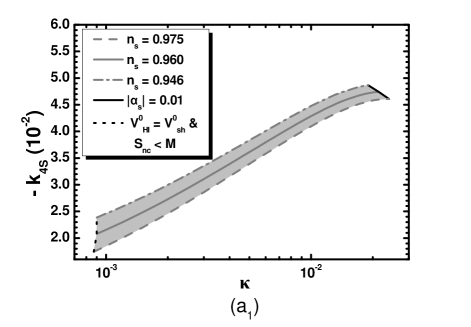
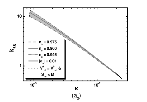
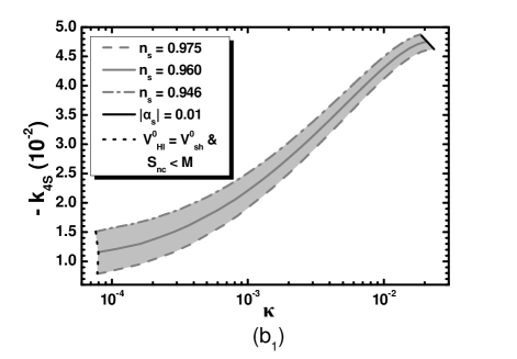
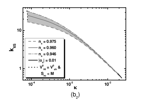
Figure 2: The (shaded) regions allowed by Eqs. (21) or (23) as well as Eqs. (34), (36), (38a), (39), and (40) in the $\kappa-(-k_{4S})$ plane (panels ${\rm a}_{1}$, ${\rm b}_{1}$) and the $\kappa-k_{6S}$ plane (panels ${\rm a}_{2}$, ${\rm b}_{2}$). We take $k_{8S}=1$ and $k_{10S}=-1$ as well as $\kappa_{T}=0.01$, $\lambda=0.1$, and $M_{T}=2.5\times 10^{16}~{}{\mbox{\rm GeV}}$ for panels ${\rm a}_{1}$, ${\rm a}_{2}$, or $\kappa_{T}=0.005$, $\lambda=0.05$, and $M_{T}=3\times 10^{16}~{}{\mbox{\rm GeV}}$ for panels ${\rm b}_{1}$, ${\rm b}_{2}$. The requirements in the paragraphs e, f, and g of Sec. IV.1 are also satisfied in these regions. The value of $n_{s}$ on the various lines is indicated.

Confronting FHI with the constraints of Sec. IV.1, we can delineate the allowed (lightly gray shaded) region in the $\kappa-(-k_{4S})$ [$\kappa-k_{6S}$] plane – see Figs. 2(${\rm a}_{1}$) and (${\rm b}_{1}$) [Figs. 2(${\rm a}_{2}$) and (${\rm b}_{2}$)]. We take $\kappa_{T}=0.01$, $\lambda=0.1$, and $M_{T}=2.5\times 10^{16}~{}{\mbox{\rm GeV}}$ for panels ${\rm a}_{1}$, ${\rm a}_{2}$ or $\kappa_{T}=0.005$, $\lambda=0.05$, and $M_{T}=3\times 10^{16}~{}{\mbox{\rm GeV}}$ for panels ${\rm b}_{1}$, ${\rm b}_{2}$. The convention adopted for the various lines is also shown in the figure. In particular, the gray dashed [dot-dashed] lines correspond to $n_{\rm s}=0.975$ [$n_{\rm s}=0.946$], whereas the gray solid lines have been obtained by fixing $n_{\rm s}=0.96$ – see Eq. (38a).

We observe that, as $\kappa$ increases, there is a remarkable augmentation of $\alpha_{\rm s}$, which saturates the bound in Eq. (39) on the thick black solid lines at the right end of the allowed regions. The inequalities in Eqs. (21) and (23) are violated to the left of the black dotted lines. The first of these inequalities, though, can remain valid at even smaller values of $\kappa$ if we take smaller values of $\kappa_{T}$ and $\lambda$ and larger values of $M_{T}$ and, thus, the dotted line is shifted to the left in this case as one can easily deduce by comparing Figs. 2(${\rm b}_{1}$) and (${\rm b}_{2}$) with Figs. 2(${\rm a}_{1}$) and (${\rm a}_{2}$). This behavior can be understood by the fact that, for such values of the parameters, the potential $V_{\rm nsh}^{0}$, which is given by Eq. (19c) – or Eq. (20) –, increases and so the bound in Eq. (21) is saturated at smaller values of $\kappa$. Note that this bound can become totally irrelevant for our calculation if we use $\kappa_{T}<0$, since, in this case, the lower bound on $\xi$ in Eq. (22) becomes extremely small and, thus, it is automatically satisfied for natural values of $\kappa$ and $\lambda$ (of order $0.1$). Would we have used $\kappa_{T}<0$ with absolute value equal to its values used in Fig. 2, the required values of $k_{4S}$ and $k_{6S}$ would have been similar to those found for $\kappa_{T}>0$ for most of the allowed values of $\kappa$ in this figure, but smaller values of $\kappa$ would also be possible. However, since the achievement of the observational constraints of Sec. IV.1 pushes $k_{6S}$ to rather high values and $\Delta_{\rm m*}$ to too small values for such small values of $\kappa$, it is not worth continuing the exploration of the parameter space in the region of such very small $\kappa$’s.

Interestingly enough, the allowed regions in Fig. 2(${\rm a}_{1}$) and (${\rm a}_{2}$) almost perfectly coincide with the allowed regions in Fig. 2(${\rm b}_{1}$) and (${\rm b}_{2}$) in their common range of $\kappa$. This signals the fact that the SUGRA corrections to $V_{\rm HI}$ originating from the two first terms in the sum in the RHS of Eq. (31) dominate over the radiative corrections in Eq. (25). The discrepancy between the various lines ranges from $2$ to $10\%$. For both sets of values of the input parameters, we see that the required values of $|k_{4S}|$ increase with $\kappa$, whereas the values of $k_{6S}$ drop. Also the mass scale $M$ increases with $\kappa$ and $M_{T}$. As we show in Sec. VI.2, $\kappa$’s lower than about $0.001$ are more preferable from the point of view of non-thermal leptogenesis and the $\widetilde{G}$ constraint. Focusing on the values of the input parameters used in Fig. 2(${\rm b}_{1}$) and (${\rm b}_{2}$), which ensure a broader allowed space, and taking $n_{\rm s}\simeq 0.96$, we find

$$0.008\lesssim\frac{\kappa}{10^{-2}}\lesssim 2.1,~{}2.64\lesssim\frac{M}{10^{16}}\lesssim 2.85,$$ (44a)

$$1.15\lesssim\frac{-k_{4S}}{10^{-2}}\lesssim 4.7,~{}~{}0.65~{}\lesssim{k_{6S}}\lesssim 25,$$ (44b)

$$0.014\lesssim\frac{-\alpha_{\rm s}}{10^{-2}}\lesssim 1,~{}~{}2.7\times 10^{-5}\lesssim\frac{r}{10^{-4}}\lesssim 2.5.~{}~{}~{}~{}~{}~{}~{}~{}$$ (44c)

In this region, the naturalness parameter $\Delta_{\rm m*}$ of the hilltop FHI ranges between $0.05$ and $0.29$. From the data used in Fig. 2, one sees that $\Delta_{\rm m*}$ increases with $\kappa$. These ranges of parameters can be further restricted imposing a number of post-inflationary requirements as we will see in Sec. VI.2.

V Non-Thermal Leptogenesis

In this section, we discuss the inflaton decay and the reheating of the universe after inflation (Sec. V.1). We also describe the scenario for generating the observed BAU in our model via a primordial non-thermal leptogenesis (Sec. V.2) consistently with the gravitino ($\widetilde{G}$) constraint gravitino ; kohri and the low energy neutrino data forero ; fogli (Sec. V.3).

V.1 The Decay of the Inflaton

Right after the termination of FHI , the inflaton field $S$ crosses $S_{\rm c}$, the trivial inflationary path in Eq. (17a) is destabilized in the $(\Phi+\bar{\Phi}^{*})/\sqrt{2}$ direction and the system is driven towards the SUSY vacuum in Eq. (5a). Soon afterwards, the system settles into a phase of damped oscillations about the SUSY vacuum and eventually decays reheating the universe. The constitution of the oscillating inflaton system (IS) can be found by constructing the neutral scalar particle spectrum at the SUSY vacuum in Eq. (5a). To this end, we expand $V_{\rm H}$ in Eq. (3) up to terms of quadratic order in the fluctuations of the fields about the vacuum and find that

$$V_{\rm H} \simeq \mbox{$\left\lgroup\begin{matrix}\delta\Phi_{+}^{*}&\delta T^{*}\end{matrix}\right\rgroup$}M^{2}_{1}\mbox{$\left\lgroup\begin{matrix}\delta\Phi_{+}\cr\delta T\end{matrix}\right\rgroup$}$$ (45)

$$+\mbox{$\left\lgroup\begin{matrix}\delta\bar{T}^{*}&\delta S^{*}\end{matrix}\right\rgroup$}M^{2}_{2}\mbox{$\left\lgroup\begin{matrix}\delta\bar{T}\cr\delta S\end{matrix}\right\rgroup$}+\cdots,$$

where the (complex) deviations of the fields $S$, $\Phi$, $\bar{\Phi}$, $T$, and $\bar{T}$ from their values in the vacuum are denoted as $\delta S$, $\delta\Phi$, $\delta\bar{\Phi}$, $\delta T$, and $\delta\bar{T}$ respectively and we have defined the complex scalar fields

$$\delta\Phi_{\pm}=\left(\delta\Phi\pm\delta\bar{\Phi}\right)/\sqrt{2}.$$ (46)

Note that the combination $\delta\Phi_{-}$ does not acquire mass from $V_{\rm H}$ in Eq. (3) as it is the Goldstone boson absorbed by the supermassive neutral gauge boson of the model. Recall that these complex scalar fields belong to the SM singlet components of the various superfields. The mass-squared matrices $M_{1}^{2}$ and $M_{2}^{2}$ in Eq. (45) are given by

$$M_{1}^{2}=\mbox{ $\left\lgroup\begin{matrix}2(\kappa^{2}+\lambda^{2})v_{\Phi}^{2}&D_{1}\cr D_{1}&M_{T}^{2}+4\kappa_{T}^{2}v_{T}^{2}\end{matrix}\right\rgroup$}$$ (47a)

with

$$D_{1}=\sqrt{2}(\lambda M_{T}-2\kappa\kappa_{T}v_{T})v_{\Phi}$$ (47b)

and

$$M_{2}^{2}=\mbox{ $\left\lgroup\begin{matrix}M_{T}^{2}+2\lambda^{2}v_{\Phi}^{2}&D_{2}\cr D_{2}&4\kappa_{T}^{2}v_{T}^{2}+2\kappa^{2}v_{\Phi}^{2}\end{matrix}\right\rgroup$}$$ (47c)

with

$$D_{2}=-2\kappa_{T}M_{T}v_{T}+2\kappa\lambda v_{\Phi}^{2}.$$ (47d)

To find the mass eigenstates of the IS, we have to diagonalize the matrices above. As it turns out, these matrices have the same eigenvalues. So, the diagonalization can be achieved via two orthogonal matrices $U_{1,2}$ as follows:

$$U_{1}M_{1}^{2}U_{1}^{\mbox{\sf\scriptsize T}}=U_{2}M_{2}^{2}U_{2}^{\mbox{\sf\scriptsize T}}=\mbox{diag}\left(m_{\rm I+}^{2},m_{\rm I-}^{2}\right),$$ (48)

where

$$m^{2}_{\rm I\pm}=\left(\bar{m}^{2}\pm D\right)/2$$ (49a)

with

$$\bar{m}^{2} = M_{T}^{2}+4\kappa_{T}^{2}v_{T}^{2}+2(\kappa^{2}+\lambda^{2})v_{\Phi}^{2},$$ (49b)

$$D^{2} = \bar{m}^{4}-8(\kappa M_{T}+2\kappa_{T}\lambda v_{T})^{2}v_{\Phi}^{2}.$$ (49c)

The matrices which diagonalize $M^{2}_{1}$ and $M^{2}_{2}$ can be cast in the form

$$U_{n}=\mbox{ $\left\lgroup\begin{matrix}V_{n+}/N_{n+}&1/N_{n+}\cr V_{n-}/N_{n-}&1/N_{n-}\end{matrix}\right\rgroup$}~{}~{}\mbox{with}~{}~{}n=1,2,$$ (50a)

where

$$V_{n\pm}=\frac{C_{n}\pm D}{2D_{n}}~{}~{}\mbox{and}~{}~{}N_{n\pm}=\sqrt{1+V^{2}_{n\pm}}.$$ (50b)

Here we use the abbreviations

$$C_{1} = -M_{T}^{2}-4\kappa_{T}^{2}v_{T}^{2}+2(\kappa^{2}+\lambda^{2})v_{\Phi}^{2},$$ (50c)

$$C_{2} = M_{T}^{2}-4\kappa_{T}^{2}v_{T}^{2}-2(\kappa^{2}-\lambda^{2})v_{\Phi}^{2}.$$ (50d)

One can show that $D^{2}=4D_{n}^{2}+C_{n}^{2}$ for $n=1$, $2$, which implies that $D^{2}$ is positive and, thus, $D$ in Eq. (49a) is a real number taken positive. Also, it is evident that the second term in RHS of Eq. (49c) is negative and, thus, the masses-squared in Eq. (49a) are both positive.

Inserting unity ($1=U_{n}U_{n}^{\mbox{\sf\scriptsize T}}=U_{n}^{\mbox{\sf\scriptsize T}}U_{n}$) on both sides of $M^{2}_{1}$ and $M_{2}^{2}$ in Eq. (45), the potential $V_{\rm H}$ can be brought into the form

$$V_{\rm H}\simeq\sum_{r=\pm}m_{{\rm I}r}^{2}\left(|\Phi_{r}|^{2}+|S_{r}|^{2}\right)+\cdots,$$ (51)

where the complex fields $\Phi_{\pm}$ and $S_{\pm}$ are given by

$$\Phi_{\pm}=\frac{\delta T+V_{1\pm}\delta\Phi_{+}}{N_{1\pm}}~{}~{}\mbox{and}~{}~{}S_{\pm}=\frac{\delta S+V_{2\pm}\delta\bar{T}}{N_{2\pm}}.$$ (52)

Solving Eq. (52) with respect to $\delta\Phi_{+}$, $\delta T$, $\delta\bar{T}$, and $\delta S$, we find

$$\delta\Phi_{+} = \frac{N_{1-}\Phi_{-}-N_{1+}\Phi_{+}}{V_{1-}-V_{1+}},~{}$$ (53a)

$$\delta T = \frac{-N_{1-}V_{1+}\Phi_{-}+N_{1+}V_{1-}\Phi_{+}}{V_{1-}-V_{1+}}$$ (53b)

and

$$\delta\bar{T} = \frac{N_{2-}S_{-}-N_{2+}S_{+}}{V_{2-}-V_{2+}},$$ (54a)

$$\delta S = \frac{-N_{2-}V_{2+}S_{-}+N_{2+}V_{2-}S_{+}}{V_{2-}-V_{2+}}\cdot$$ (54b)

After the end of FHI, each of the four complex scalar fields $\Phi_{\pm}$ and $S_{\pm}$ oscillates about the SUSY vacuum and decays into a pair of right-handed sneutrinos ($\nu^{c}_{i}$) or neutrinos ($\psi_{\nu^{c}_{i}}$). The masses of these (s)neutrinos are generated, after the breaking of $G_{\rm LR}$, by the first term in the RHS of Eq. (10) and turn out to be

$$M_{{[}\nu^{c}}i]=2{\lambda_{i\nu^{c}}v_{\Phi}^{2}/M_{\rm S}}.$$ (55)

Here we assumed that the superfields $l^{c}_{i}$ have been rotated in the family space so that the coupling constant matrix $\lambda_{ij}$ in Eq. (10) becomes diagonal with real and positive eigenvalues $\lambda_{i\nu^{c}}$. This is the so-called dent right-handed neutrino basis, where the right-handed neutrino masses are diagonal, real, and positive. The first coupling in the RHS of Eq. (10) together with the superpotential terms in Eq. (2) also leads to the decay of the IS to a pair of right-handed neutrinos or sneutrinos. In particular, from this coupling, we obtain the following Lagrangian term (note that the decay of $T$ via the two last terms in the RHS of Eq. (6) is kinematically blocked):

$${\cal L}_{\Phi T} = -\sqrt{2}\lambda_{i\nu^{c}}\frac{v_{\Phi}}{M_{\rm S}}\delta\Phi_{+}\psi_{\nu_{i}^{c}}\psi_{\nu_{i}^{c}}+{\rm H.c.}$$ (56a)

$$= -\lambda_{i}\sum_{r=\pm}\gamma_{\Phi r}\Phi_{r}\psi_{\nu_{i}^{c}}\psi_{\nu_{i}^{c}}+{\rm H.c.},$$

where

$$\lambda_{i}=\sqrt{2}\lambda_{i\nu^{c}}v_{\Phi}/M_{\rm S}$$ (56b)

and

$$\gamma_{\Phi r}=\left\{\begin{matrix}-&N_{1+}/(V_{1-}-V_{1+})~{}~{}\mbox{for}~{}~{}&r=+\cr&N_{1-}/(V_{1-}-V_{1+})~{}~{}\mbox{for}~{}~{}&r=-~{},\cr\end{matrix}\right.$$ (56c)

as one finds using Eq. (53a).

Moreover, from the F-term $(\partial W_{\rm H}/\partial\bar{\Phi})^{*}(\partial W_{\rm NR}/\partial\bar{\Phi})+{\rm H.c.}$ with $W_{\rm H}$ and $W_{\rm NR}$ in Eqs. (2) and (10) respectively, we obtain the Lagrangian terms

$${\cal L}_{S\bar{T}} = -2v_{\Phi}\lambda_{i\nu^{c}}\frac{v_{\Phi}}{M_{\rm S}}\left(\kappa S^{*}+\lambda\bar{T}^{*}\right)\nu^{c}_{i}\nu^{c}_{i}+{\rm H.c.}$$ (57a)

$$= -\lambda_{i}\sum_{r=\pm}\gamma_{Sr}S_{r}m_{{\rm I}r}\nu^{c}_{i}\nu^{c}_{i}+{\rm H.c.},$$

where the $$\gamma_{Sr}$$’s can be derived from Eqs. (54a) and (54b) and turn out to be

$$\gamma_{S+} = \frac{\sqrt{2}v_{\Phi}\left(\kappa N_{2+}V_{2-}-\lambda N_{2+}\right)}{m_{{\rm I}+}\left(V_{2-}-V_{2+}\right)},$$ (57b)

$$\gamma_{S-} = \frac{\sqrt{2}v_{\Phi}\left(-\kappa N_{2-}V_{2+}+\lambda N_{2-}\right)}{m_{{\rm I}-}\left(V_{2-}-V_{2+}\right)}.$$ (57c)

For $m_{{\rm I}\pm}\gg M_{{[}\nu^{c}}i]$, the Lagrangians ${\cal L}_{\Phi T}$ and ${\cal L}_{S\bar{T}}$ in Eqs. (56a) and (57a) give rise to a common decay width $\Gamma_{[}\rm I+\rightarrow\nu^{c}_{i}]$ for $\Phi_{+}$ to a pair of right-handed neutrinos $\psi_{\nu_{i}^{c}}$ and $S_{+}$ to a pair of right-handed sneutrinos $\nu^{c}_{i}$ and a different common decay width $\Gamma_{[}\rm I-\rightarrow\nu^{c}_{i}]$ for $\Phi_{-}$ to a pair of right-handed neutrinos $\psi_{\nu_{i}^{c}}$ and $S_{-}$ to a pair of right-handed sneutrinos $\nu^{c}_{i}$:

$$\Gamma_{[}\rm I\pm\rightarrow\nu^{c}_{i}]\simeq\frac{1}{32\pi}\lambda_{i}^{2}\,\gamma_{\Phi\pm}^{2}m_{{\rm I}\pm}=\frac{1}{32\pi}\lambda_{i}^{2}\,\gamma_{S\pm}^{2}m_{{\rm I}\pm}.$$ (58)

The inflaton subsystem consisting of $\Phi_{+}$ and $S_{+}$ will be called the I₊ subsystem, while the one consisting of $\Phi_{-}$ and $S_{-}$ will be called the I_- subsystem. We checked numerically that the widths of the SUGRA-induced Idecay decay channels of the IS are negligible in our model for the values of $v_{\Phi}$ and $m_{\rm I-}$ obtained in Sec. IV.2 and, therefore, we do not include these channels in our calculation. Since the decay width of the produced $\nu^{c}_{i}$ is much larger than $\Gamma_{[}{\rm I}\pm\rightarrow\nu^{c}_{i}]$ – see below – the reheating temperature $T_{\rm rh}$ is exclusively determined by the decay of the IS and is given by quin

$$T_{\rm rh}=\left(\frac{72}{5\pi^{2}g_{*}}\right)^{1/4}\sqrt{m_{\rm P}\Gamma_{[}{\rm I}-]},~{}~{}\mbox{where}~{}~{}\Gamma_{[}{\rm I}\pm]=\mbox{$\sum_{i}$}\Gamma_{[}\rm I\pm\rightarrow\nu^{c}_{i}].$$ (59)

Here $g_{*}$ counts the effective number of relativistic degrees of freedom at temperature $T_{\rm rh}$ and we assumed that $\Gamma_{[}{\rm I}-]\ll\Gamma_{[}{\rm I}+]$. For the MSSM spectrum plus the particle content of the superfields $N$ and $\bar{N}$, we find that $g_{*}\simeq 228.75+4(1+7/8)=236.25$.

V.2 Lepton Asymmetry and Gravitino Abundance

The implementation of non-thermal leptogenesis requires that the right-handed (s)neutrinos which emerge at reheating decay out-of-equilibrium baryo to light particles. This condition is automatically satisfied provided that $T_{\rm rh}\ll M_{{[}\nu^{c}}i]$. The superfield $\nu^{c}_{i}$ decays into a right-handed Higgs superfield and a ${\rm SU(2)_{L}}$ doublet right-handed antilepton superfield via the tree-level Yukawa couplings derived from the second term in the RHS of Eq. (7). Interference between tree-level and one-loop diagrams generates a lepton-number asymmetry $\varepsilon_{i}$ per $\nu^{c}_{i}$ decay baryo provided that CP is violated. The resulting overall lepton-number asymmetry $Y_{L}\equiv n_{L}/s$ ($n_{L}$ is the lepton-number density and $s$ the entropy density) after reheating is given by

$$Y_{L}=2\frac{5}{4}\frac{T_{\rm rh}}{m_{\rm I-}}\mbox{$\sum_{i}$}\frac{\Gamma_{[}{\rm I-}\rightarrow\nu^{c}_{i}]}{\Gamma_{[}{\rm I}-]}\varepsilon_{i}$$ (60a)

and can be partially converted via electroweak sphaleron effects into baryon-number asymmetry which, in MSSM, is estimated to be

$$Y_{B}=-0.35Y_{L}.$$ (60b)

The factor 2 in the RHS of Eq. (60a) comes from the fact that each decaying inflaton gives two right-handed (s)neutrinos, whereas the factor ($5/4$) is consistent with the calculation of $T_{\rm rh}$ in Ref. quin , which leads to Eq. (59). Finally, the numerical factor in the RHS of Eq. (60b) originates ibanez from the electroweak sphaleron effects.

We should, however, keep in mind that, if the lightest right-handed neutrino mass $M_{1\nu^{c}}$ is less than about $10T_{\rm rh}$, $Y_{L}$ can be partly washed out due to $\nu^{c}_{1}$ mediated inverse decay and $\Delta L=1$ scattering processes – this possibility is analyzed in Ref. senoguz . In order to avoid the computational complications related to this washout, we limit ourselves to cases with $M_{{[}\nu^{c}}1]\gtrsim 10T_{\rm rh}$ so that no washout of the non-thermally produced $Y_{L}$ occurs. Moreover, $Y_{L}$ is not erased by $\Delta L=2$ scattering processes erasure at all temperatures $T$ between $100~{}{\mbox{\rm GeV}}$ and $T_{\rm rh}$ since $Y_{L}$ is automatically protected by SUSY ibanez for $10^{7}~{}{\mbox{\rm GeV}}\lesssim T\lesssim T_{\rm rh}$ and for $T\lesssim 10^{7}~{}{\mbox{\rm GeV}}$ these processes are well out of equilibrium provided that the mass of the heaviest light neutrino is smaller than about $10~{}{\mbox{\rm eV}}$. This constraint, however, is overshadowed by a more stringent restriction induced by the current data wmap ; plcp – see Sec. VI.

The reheat temperature $T_{\rm rh}$ must be compatible with the constraint on the $\widetilde{G}$ abundance $Y_{\widetilde{G}}$ at the onset of big bang nucleosynthesis (BBN). This abundance is estimated to be kohri

$$Y_{\widetilde{G}}\simeq 1.9\cdot 10^{-22}~{}T_{\rm rh}/{\mbox{\rm GeV}},$$ (61)

where we assume that $\widetilde{G}$ is much heavier than the gauginos. Note that non-thermal $\widetilde{G}$ production is Idecay also possible within SUGRA. However, we adopt here the conservative estimate of $Y_{\widetilde{G}}$ in Eq. (61) since this non-thermal production of gravitinos depends on the mechanism of SUSY breaking. It is important to mention that Eqs. (60b) and (61) give the correct values of baryon asymmetry and $\widetilde{G}$ abundance provided that no entropy production occurs at $T<T_{\rm rh}$. This requirement can be very easily achieved within our setting.

The mass spectrum of the $N$-$\bar{N}$ system – see second term in Eq. (10) – consists of a saxion and an axion corresponding, respectively, to the real and the imaginary part of the complex scalar field $N_{-}=(\delta N-\delta\bar{N})/\sqrt{2}$, an axino $\psi_{-}=(\psi_{N}-\psi_{\bar{N}})/\sqrt{2}$, two extra real Higgs fields corresponding to the real and the imaginary part of $N_{+}=(\delta N+\delta\bar{N})/\sqrt{2}$, and an extra Higgsino $\psi_{N+}=(\psi_{N}+\psi_{\bar{N}})/\sqrt{2}$ all with masses of order $1~{}\rm TeV$ except, of course, the axion which is very light ($\delta N$, $\delta\bar{N}$ are, respectively, the complex deviations of $N$, $\bar{N}$ from their VEVs and $\psi$ denotes a Weyl spinor).

The extra Higgs fields and the extra Higgsino can decay, if this is kinematically allowed, to ordinary Higgs fields and Higgsinos before dominating the universe curvaton . However, under certain conditions, the extra Higgsino can contribute to the cold dark matter (CDM) in the universe antonio .

Regarding the saxion in $N_{-}$, we can assume that its decay mode to axions is suppressed with respect to its decay modes to gluons, Higgses, and Higgsinos Baer ; senami and the initial amplitude of its oscillations is approximately equal to the axion decay constant $f_{a}\simeq 10^{12}~{}{\mbox{\rm GeV}}$. Under these circumstances, the saxion can Baer decay before dominating the universe and the stringent upper bound on $T_{\rm rh}$ from the limit on the effective number of neutrinos at BBN is alleviated senami . As a consequence of the relatively large decay temperature of the saxion, the resulting lightest sparticles (LSPs) are likely to be thermalized and, therefore, no upper bound on the saxion abundance and, thus, $T_{\rm rh}$ is obtained senami .

The axions could in principle contribute to dark matter, but we should keep in mind that they generate isocurvature perturbations – see e.g. Refs. curvaton ; lchios – which are strongly restricted by the present data from the Planck satellite plin . Indeed, since, in our model, the PQ symmetry must be broken during FHI – see Ref. curvaton –, the axion acquires quantum fluctuations as all the almost massless degrees of freedom. At the QCD phase transition, these fluctuations turn into isocurvature perturbations in the axion energy density, which means that the partial curvature perturbation in axions is different than the one in photons. Therefore, a large axion contribution to CDM is disfavored within our model.

Finally, the axino cannot be the LSP because its large expected mass and the relatively high $T_{\rm rh}$’s encountered here would then lead bae to an unacceptably large CDM abundance. Nonetheless, the axino may bae enhance non-thermally the abundance of a neutralino LSP which is a successful CDM candidate.

V.3 Leptogenesis and Low Energy Neutrino Data

As mentioned above, the decay of a right-handed sneutrino $\nu^{c}_{i}$ or neutrino $\psi_{\nu^{c}_{i}}$ emerging from the IS decay at reheating can generate a lepton asymmetry $\varepsilon_{i}$ due to the interference between the tree-level and the one-loop decay diagrams as well as the violation of the CP symmetry. The generated $\varepsilon_{i}$ can be expressed in terms of the Dirac mass matrix $m^{\rm D}_{\nu}$ of the neutrinos defined in the right-handed neutrino basis:

$$\varepsilon_{i}=\sum_{j\neq i}\frac{{\sf Im}\left[(m_{\nu}^{{\rm D}{\dagger}}m^{\rm D}_{\nu})_{ij}^{2}\right]}{8\pi\langle{H_{2}}\rangle^{2}(m_{\nu}^{{\rm D}{\dagger}}m_{\nu}^{\rm D})_{ii}}\bigg{(}F_{\rm V}(x_{ij})+F_{\rm S}(x_{ij})\bigg{)},$$ (62a)

where

$$x_{ij}\equiv\frac{M_{{[}\nu^{c}}j]}{M_{{[}\nu^{c}}i]}$$ (62b)

and $$\langle{H_{2}}\rangle\simeq 174~{}{\mbox{\rm GeV}} \tan\beta F_{\rm V} F_{\rm S}$$ assuming large . Also and represent, respectively, the contributions from the vertex and self-energy diagrams and, in SUSY theories, are given covi by

$$F_{\rm V}\left(x\right) = -x\ln\left(1+x^{-2}\right),$$ (62c)

$$F_{\rm S}\left(x\right) = -\frac{2x}{x^{2}-1}\cdot$$ (62d)

Note that Eqs. (62a), (62c), and (62d) hold provided that the right-handed neutrinos are far from being degenerate, which is true in our case. In particular, for strongly hierarchical $M_{{[}\nu^{c}}i]$’s with $x_{ij}\gg 1$, $j\neq i$, we obtain the well-known approximate result frigerio ; senoguz

$$F_{\rm V}+F_{\rm S}\simeq-\frac{3}{x_{ij}^{2}}\cdot$$ (63)

The Dirac mass matrix $m_{\nu}^{\rm D}$ in Eq. (62a) is diagonalized in the so-called dent weak basis, in which the lepton Yukawa couplings and the ${\rm SU(2)_{L}}$ interactions are diagonal in the generation space. In particular, we have

$$U^{\dagger}m_{\nu}^{\rm D}U^{c{\dagger}}\equiv d^{\rm D}={\sf diag}\left(m^{\rm D}_{1},m^{\rm D}_{2},m^{\rm D}_{3}\right),$$ (64)

where $m^{\rm D}_{1}$, $m^{\rm D}_{2}$, and $m^{\rm D}_{3}$ are real and positive and $U$ and $U^{c}$ are $3\times 3$ unitary matrices which relate $l_{i}$ and $\nu^{c}_{i}$ in the right-handed neutrino basis with $l^{\prime}_{i}$ and $\nu^{c\prime}_{i}$ in the weak basis as follows:

$$l^{\prime}=lU\>\>\>\mbox{and}\>\>\>\nu^{c\prime}=U^{c}\nu^{c}.$$ (65)

Here, we write the left-handed ${\rm SU(2)_{L}}$ doublet lepton superfields as row 3-vectors in family space and the right-handed ${\rm SU(2)_{L}}$ singlet antilepton superfields as column 3-vectors. The matrix $m_{\nu}^{{\rm D}{\dagger}}m_{\nu}^{\rm D}$ in Eq. (62a) then becomes a function of $d^{\rm D}$ and $U^{c}$. Namely,

$$m_{\nu}^{{\rm D}{\dagger}}m_{\nu}^{\rm D}=U^{c{\dagger}}d^{{\rm D}{\dagger}}d^{\rm D}U^{c}.$$ (66)

The non-thermal leptogenesis scenario depends on the low energy neutrino data via the seesaw formula, which gives the light-neutrino mass matrix $m_{\nu}$ in terms of $m^{\rm D}_{i}$ and $M_{{[}\nu^{c}}i]$. In the right-handed neutrino basis, the seesaw formula becomes

$$m_{\nu}=-m^{\rm D}_{\nu}\ d_{\nu^{c}}^{-1}\ \left(m_{\nu}^{\rm D}\right)^{{\mbox{\sf\scriptsize T}}},$$ (67a)

where

$$d_{\nu^{c}}={\sf diag}\left(M_{{[}\nu^{c}}1],M_{{[}\nu^{c}}2],M_{{[}\nu^{c}}3]\right)$$ (67b)

with $M_{{[}\nu^{c}}1]\leq M_{{[}\nu^{c}}2]\leq M_{{[}\nu^{c}}3]$ real and positive. Solving Eq. (64) with respect to $m_{\nu}^{\rm D}$ and inserting the resulting expression in Eq. (67a), we find that the light neutrino mass matrix in the weak basis is given by

$$\bar{m}_{\nu}=U^{\dagger}m_{\nu}U^{*}=-d^{\rm D}U^{c}d_{\nu^{c}}^{-1}U^{c{\mbox{\sf\scriptsize T}}}d^{\rm D}.$$ (68)

This mass matrix can be diagonalized by the unitary Pontecorvo-Maki-Nakagawa-Sakata (PMNS) matrix $U_{\nu}$:

$$U_{\nu}^{{\mbox{\sf\scriptsize T}}}\bar{m}_{\nu}U_{\nu}={\sf diag}\left(m_{[\nu}1],m_{[\nu}2],m_{[\nu}3]\right)\$$ (69)

with $m_{[\nu}1]$, $m_{[\nu}2]$, and $m_{[\nu}3]$ being the real and positive light neutrino mass eigenvalues and the PMNS matrix $U_{\nu}$ parametrized as follows:

$$U_{\nu}=\left\lgroup\begin{matrix}c_{12}c_{13}&s_{12}c_{13}&s_{13}e^{-i\delta}\cr U_{21\nu}&U_{22\nu}&s_{23}c_{13}\cr U_{31\nu}&U_{32\nu}&c_{23}c_{13}\end{matrix}\right\rgroup\cdot{\cal P}.$$ (70)

Here

$$U_{21\nu} = -c_{23}s_{12}-s_{23}c_{12}s_{13}e^{i\delta},$$ (71a)

$$U_{22\nu} = c_{23}c_{12}-s_{23}s_{12}s_{13}e^{i\delta},$$ (71b)

$$U_{31\nu} = s_{23}s_{12}-c_{23}c_{12}s_{13}e^{i\delta},$$ (71c)

$$U_{32\nu} = -s_{23}c_{12}-c_{23}s_{12}s_{13}e^{i\delta},$$ (71d)

where $c_{ij}\equiv\cos\theta_{ij}$, $s_{ij}\equiv\sin\theta_{ij}$ with $\theta_{ij}$ being the appropriate mixing angles and $\delta$ is the CP-violating Dirac phase. The two CP-violating Majorana phases $\varphi_{1}$ and $\varphi_{2}$ are contained in the matrix

$${\cal P}={\sf diag}\left(e^{-i\varphi_{1}/2},e^{-i\varphi_{2}/2},1\right).$$ (72)

Following a bottom-up approach along the lines of Refs. frigerio ; senoguz , we find $\bar{m}_{\nu}$ via Eq. (69) using as input parameters the low energy neutrino observables for various values of $m_{1\nu}$ and the CP-violating Majorana phases $\varphi_{1}$ and $\varphi_{2}$ and adopting the normal or inverted hierarchical scheme of light neutrino masses – see Sec. VI.1. Taking also $m^{\rm D}_{i}$ as input parameters, we construct the complex symmetric matrix

$$W=-(d^{\rm D})^{-1}\bar{m}_{\nu}(d^{\rm D})^{-1}=U^{c}d_{\nu^{c}}^{-1}U^{c{\mbox{\sf\scriptsize T}}}$$ (73)

– see Eq. (68) – from which we can extract $d_{\nu^{c}}$ as follows:

$$d_{\nu^{c}}^{-2}=U^{c{\dagger}}WW^{\dagger}U^{c}.$$ (74)

Note that $WW^{\dagger}$ is a $3\times 3$ complex, Hermitian matrix and is diagonalized following the algorithm described in Ref. 33m so as to determine the elements of $U^{c}$ and the $M_{{[}\nu^{c}}i]$’s. We then compute $m_{\nu}^{{\rm D}{\dagger}}m^{\rm D}_{\nu}$ through Eq. (66) and the $\varepsilon_{i}$’s via Eq. (62a).

VI Updating the Constraints on the Model Parameters

The parameters of our model can be further restricted if, in addition to the inflationary requirements mentioned in Sec. IV.1, we impose extra constraints arising from the post-inflationary evolution predicted by our model. These constraints are outlined in Sec. VI.1, whereas, in Sec. VI.2, we derive the overall allowed parameter space of our model.

VI.1 Post-Inflationary Requirements

We summarize below the requirements which guarantee a successful post-inflationary evolution in our scheme:

We require the following bounds on $M_{{[}\nu^{c}}i]$:

$$M_{{[}\nu^{c}}i]\lesssim 7.1\frac{v_{\Phi}^{2}}{M_{\rm S}},\>\>M_{{[}\nu^{c}}1]\gtrsim 10\,T_{\rm rh},\>\>\mbox{and}\>\>m_{\rm I-}\geq 2M_{{[}\nu^{c}}1].$$ (75)

The first bound ensures that the coupling constants $\lambda_{i\nu^{c}}$ in Eqs. (10) and (55) acquire perturbative values, i.e. $\lambda_{i\nu^{c}}^{2}/4\pi\leq 1$. The second inequality is applied in order to protect the generated lepton asymmetry $Y_{L}$ against any possible washout by $\nu^{c}_{1}$-mediated inverse decay and $\Delta L=1$ scattering processes as mentioned in Sec. V.2 – see Ref. senoguz . Finally, the last bound ensures that the decay of the IS to a pair of $\nu^{c}_{i}$’s is kinematically allowed for at least one species of the $\nu^{c}_{i}$’s.

The Dirac masses $m^{\rm D}_{i}$ selected for $\nu_{i}$ at $M_{\rm GUT}$ need to be consistent with the relations in Eqs. (15c) and (15d). In order to reduce the number of free parameters and simplify the relevant constraint, we assume that $y_{ijL}$ and $y^{\prime}_{ijL}$ are simultaneously diagonal in the weak basis with elements $y_{iL}$ and $y^{\prime}_{iL}$ respectively. Under this assumption, we have to check that the selected $m^{\rm D}_{i}$’s can be obtained together with the masses $m_{iE}$ of the charged leptons by a natural set of $y_{iL}$’s and $y^{\prime}_{iL}$’s with $a_{1}$ and $a_{2}$ of order unity. In other words, the solution of the six by six system of equations

$$\frac{y_{iL}-\alpha_{2}y^{\prime}_{iL}}{\sqrt{1+|\alpha_{2}|^{2}}}\,v_{2}=m^{\rm D}_{i},~{}~{}\frac{y_{iL}-\alpha_{1}y^{\prime}_{iL}}{\sqrt{1+|\alpha_{1}|^{2}}}\,v_{1}=m_{iE}$$ (76)

has to exist and be natural for a set of natural values of $a_{1}$ and $a_{2}$. Here we put $v_{1}=174\cos\beta~{}{\mbox{\rm GeV}}$ and $v_{2}=174\sin\beta~{}{\mbox{\rm GeV}}$, and $m_{iE}$ and $m^{\rm D}_{i}$ are taken at $M_{\rm GUT}$ assuming that the running from $M_{\rm GUT}$ until the scale of non-thermal leptogenesis $\Lambda_{L}$, which is taken to be $\Lambda_{L}=m_{\rm I-}$, is negligible. Working in the context of MSSM with universal gaugino masses and $\tan\beta\simeq 50$ – favored by the recent results of LHC higgs on the lightest Higgs boson mass – and taking into account the SUSY threshold corrections, we obtain fermionM

$$\hskip 59.75095pt(m_{1E},m_{2E},m_{3E})=$$

$$(0.39-0.532,83.5-112.7,1635-2400)~{}\rm MeV.~{}~{}~{}$$ (77)

From the solar, atmospheric, accelerator, and reactor neutrino experiments, we take as inputs in our calculation the best-fit values forero – see also Ref. fogli –

$$\Delta m^{2}_{21} = 7.62\times 10^{-3}~{}{\rm eV}^{2},$$ (78a)

$$\Delta m^{2}_{31} = 2.55\left[-2.43\right]\times 10^{-3}~{}{\rm eV}^{2}$$ (78b)

for the differences $$\Delta m^{2}_{ij}\equiv m^{2}_{i\nu}-m^{2}_{j\nu}$$ between the light neutrino masses-squared,

$$\sin^{2}\theta_{12} = 0.32,$$ (78c)

$$\sin^{2}\theta_{13} = 0.0246\left[0.025\right],$$ (78d)

$$\sin^{2}\theta_{23} = 0.613\left[0.6\right]$$ (78e)

for the mixing angles, and

$$\delta=0.8\pi\left[-0.03\pi\right]$$ (78f)

for the CP-violating Dirac phase in the case of normal [inverted] neutrino mass hierarchy. In particular, two of the $m_{[\nu}i]$’s are determined in terms of the third one using the relation

$$m_{[\nu}2]=\sqrt{m_{[\nu}1]^{2}+\Delta m^{2}_{21}}$$ (79a)

and either

$$m_{[\nu}3]=\sqrt{m_{[\nu}1]^{2}+\Delta m^{2}_{31}}$$ (79b)

for normally ordered (NO) $$m_{[\nu}i]$$’s or

$$m_{[\nu}1]=\sqrt{m_{[\nu}3]^{2}+\left|\Delta m^{2}_{31}\right|}$$ (79c)

for invertedly ordered (IO) $m_{[\nu}i]$’s. We also take into account the fact that the sum of the $m_{[\nu}i]$’s is bounded above by the current data wmap ; plcp :

$$\mbox{$\sum_{i}$}m_{[\nu}i]\leq 0.28~{}{{\mbox{\rm eV}}}$$ (80)

at 95% c.l.

The BAU $Y_{B}$ must satisfy the constraint plcp

$$Y_{B}\simeq\left(8.55\pm 0.217\right)\times 10^{-11}~{}~{}\mbox{at 95\% c.l.}$$ (81)

To avoid spoiling the success of the BBN, an upper bound on $Y_{\widetilde{G}}$ must be imposed depending on the $\widetilde{G}$ mass $m_{\widetilde{G}}$ and the dominant $\widetilde{G}$ decay mode. We consider here the conservative case where $\widetilde{G}$ decays with a tiny hadronic branching ratio. In this case, we have kohri

$$Y_{\widetilde{G}}\lesssim\left\{\begin{matrix}10^{-14}\hfill\cr 10^{-13}\hfill\cr 10^{-12}\hfill\cr\end{matrix}\right.\>\>\>\mbox{for}\>\>\>m_{\widetilde{G}}\simeq\left\{\begin{matrix}0.69~{}{\rm TeV}\hfill\cr 10.6~{}{\rm TeV}\hfill\cr 13.5~{}{\rm TeV}.\hfill\cr\end{matrix}\right.$$ (82)

VI.2 Results

The inflationary requirements of Sec. III restrict $k_{4S}$ and $k_{6S}$ as functions of $\kappa$ for given $\lambda$, $\kappa_{T}$, and $M_{T}$. We first concentrate on a low value of $\kappa$ within its allowed range. This ensures a low enough $m_{\rm I-}$ through Eq. (49a). As a consequence, $Y_{B}$ in Eq. (60b) is enhanced, whereas $T_{\rm rh}$ is kept sufficiently low, as can be deduced from Eqs. (58) and (59). Namely, we take $\kappa=0.001$, $\kappa_{T}=0.01$, $\lambda=0.1$, $M_{T}=2.5\times 10^{16}~{}{\mbox{\rm GeV}}$, $k_{4S}=-0.0215$, and $k_{6S}=10.9$ yielding $m_{\rm I-}=2.94\times 10^{13}~{}{\mbox{\rm GeV}}$.

Note that $T_{\rm rh}$ and $Y_{B}$ depend also on the masses $M_{{[}\nu^{c}}i]$ of the $\nu^{c}_{i}$’s into which ${\rm I}_{-}$ decays. In addition, $Y_{B}$ depends crucially on the low energy parameters related to neutrino physics. Following a bottom-up approach, we find the $M_{{[}\nu^{c}}i]$’s by using as input parameters the $m^{\rm D}_{i}$’s, the mass of one of the $\nu_{i}$’s – the $m_{[\nu}1]$ for NO $m_{[\nu}i]$’s, or the $m_{[\nu}3]$ for IO $m_{[\nu}i]$’s –, the two Majorana phases $\varphi_{1}$ and $\varphi_{2}$ of the PMNS matrix, and the best-fit values – see Eqs. (78a)-(78f) – of the low energy neutrino parameters. In our numerical code, we run these best-fit values up to the scale of non-thermal leptogenesis $\Lambda_{L}=m_{\rm I-}$ following Ref. running and considering the MSSM with $\tan\beta\simeq 50$ as an effective theory between the soft SUSY-breaking scale $M_{\rm SUSY}=1.5~{}\rm TeV$ and $\Lambda_{L}$. The so obtained $M_{{[}\nu^{c}}i]$’s clearly correspond to the scale $\Lambda_{L}$.

Our results are displayed in Table 3 for some representative values of the parameters which yield acceptable $Y_{B}$ and $Y_{\widetilde{G}}$, i.e. lying in the ranges shown in Eqs. (81) and (82). We consider strongly NO (cases A and B), almost degenerate (cases C, D, and E) and strongly IO (cases F and G) neutrino masses. Note that the cases C and D correspond to NO $m_{[\nu}i]$’s with large $m_{[\nu}1]$, while the case E corresponds to IO $m_{[\nu}i]$’s with large $m_{[\nu}3]$. In all these cases, the current limit – see Eq. (80) – on the sum of the $m_{[\nu}i]$’s is safely met – in the case D, this limit is almost saturated. Care is taken, in addition, so that the first inequality of Eq. (75) is satisfied. Our choice to use the effective scale $M_{S}$ in Eq. (10) helps in this direction. Indeed, have we chosen this effective scale to be equal to $m_{\rm P}$, the case A in Table 3 would be excluded due to the violation of this inequality. We also observe that with strongly NO or IO $m_{[\nu}i]$’s the resulting $M_{{[}\nu^{c}}i]$’s are strongly hierarchical. With almost degenerate $m_{[\nu}i]$’s, though, the resulting $M_{i\nu}$’s are closer to one another. As a consequence, in this case, more ${\rm I}_{-}$-decay channels are, generally, available. In the case A, only a single decay channel is open. In all the other cases, the dominant contribution to $Y_{B}$ arise from $\varepsilon_{2}$ – recall Eqs. (60a) and (60b). In Table 3, we also display, for comparison, the $B$ abundance with ($Y_{B}$) or without ($Y^{0}_{B}$) taking into account the renormalization group running of the low energy neutrino data. We observe that the two results are in most cases close to each other with the biggest discrepancy encountered in the case E of almost degenerate IO $m_{[\nu}i]$’s. Shown are also the values of $T_{\rm rh}$, the majority of which are close to $5\times 10^{8}~{}{\mbox{\rm GeV}}$, and the corresponding $Y_{\widetilde{G}}$’s, which, in most of the cases, are consistent with Eq. (82) only for large values of $m_{\widetilde{G}}\gtrsim 10~{}\rm TeV$. Thus, from the perspective of the $\widetilde{G}$ constraint, the case A turns out to be the most promising one.

Table 3: Parameters yielding acceptable BAU for $\kappa=0.001$, $\kappa_{T}=0.01$, $\lambda=0.1$, $M_{T}=2.5\times 10^{16}~{}{\mbox{\rm GeV}}$, $k_{4S}=-0.0215$, $k_{6S}=10.9$, and various neutrino mass schemes.

Parameters	Cases
	A	B	C	D	E	F	G
	Normally		Almost			Invertedly
	Ordered		Degenerate			Ordered
	$\nu$ Masses		$\nu$ Masses			$\nu$ Masses
Low Energy Neutrino Parameters
$m_{[\nu}1]/0.1~{}{\mbox{\rm eV}}$	$0.01$	$0.1$	$0.5$	$0.7$	$0.7$	$0.5$	$0.49$
$m_{[\nu}2]/0.1~{}{\mbox{\rm eV}}$	$0.09$	$0.1$	$0.5$	$0.7$	$0.7$	$0.51$	$0.5$
$m_{[\nu}3]/0.1~{}{\mbox{\rm eV}}$	$0.5$	$0.5$	$0.7$	$0.86$	$0.5$	$0.1$	$0.05$
$\sum_{i}m_{[\nu}i]/0.1~{}{\mbox{\rm eV}}$	$0.6$	$0.7$	$1.7$	$2.3$	$1.9$	$1.1$	$1$
$\varphi_{1}$	$\pi/3$	$\pi/2$	$0$	$\pi/2$	$\pi$	$-\pi/3$	$-\pi/2$
$\varphi_{2}$	$0$	$0$	$3\pi/4$	$\pi/2$	$\pi$	$-\pi/2$	$-\pi/6$
Mass Parameters at the Leptogenesis Scale
$m^{\rm D}_{1}/0.1~{}{\mbox{\rm GeV}}$	$4.7$	$4.1$	$15.5$	$10$	$7$	$9.5$	$7$
$m^{\rm D}_{2}/{\mbox{\rm GeV}}$	$26$	$2.3$	$2$	$2.5$	$1.2$	$1.4$	$2$
$m^{\rm D}_{3}/10~{}{\mbox{\rm GeV}}$	$12$	$12$	$5$	$8$	$0.4$	$12$	$1.5$
$M_{{[}\nu^{c}}1]/10^{10}~{}{\mbox{\rm GeV}}$	$5.9$	$2.2$	$4.9$	$1.4$	$0.67$	$1.7$	$1$
$M_{{[}\nu^{c}}2]/10^{11}~{}{\mbox{\rm GeV}}$	$177$	$1.4$	$1$	$0.94$	$0.069$	$0.8$	$1.5$
$M_{{[}\nu^{c}}3]/10^{13}~{}{\mbox{\rm GeV}}$	$342$	$45$	$1.9$	$5.3$	$0.007$	$51$	$1.7$
Decay Channels of the Inflaton ${\rm I}_{-}$ with mass $m_{\rm I-}$
I${}_{-}\rightarrow$	$\nu^{c}_{[}1]$	$\nu^{c}_{[}1,2]$	$\nu^{c}_{[}1,2]$	$\nu^{c}_{[}1,2]$	$\nu^{c}_{[}1,2,3]$	$\nu^{c}_{[}1,2]$	$\nu^{c}_{[}1,2]$
Resulting Baryon Asymmetry
$10^{11}Y^{0}_{B}$	$8.72$	$7.45$	$7.98$	$7.96$	$5.5$	$7.97$	$7.97$
$10^{11}Y_{B}$	$8.53$	$8.23$	$8.4$	$8.64$	$8.78$	$8.6$	$8.53$
Resulting $T_{\rm rh}$ and $\widetilde{G}$ Abundance
$T_{\rm rh}/10^{8}~{}{\mbox{\rm GeV}}$	$3.4$	$8$	$6.8$	$5.6$	$5.9$	$4.9$	$8.7$
$10^{13}Y_{\widetilde{G}}$	$0.7$	$1.5$	$1.3$	$1$	$1.1$	$0.9$	$1.65$

As we emphasize in Sec. II, the inclusion in our model of the $T$ and $\bar{T}$ superfields – which has various consequences for the inflationary scenario (see Sec. III) – is of crucial importance for the violation of the partial YU and the tight constraint on the Dirac neutrino masses $m^{\rm D}_{i}$’s predicted by the simplest left-right symmetric model. Indeed, in the simplest model, where $\alpha_{1}=\alpha_{2}$, and for the central values of the $m_{iE}$’s in Eq. (77), we would have the following values of the $m^{\rm D}_{i}$’s:

$$\left(m^{0{\rm D}}_{1},m^{0{\rm D}}_{2},m^{0{\rm D}}_{3}\right)\simeq(0.023,4.9,100)~{}{\mbox{\rm GeV}}.$$ (83)

However, in sharp contrast with Eq. (83), in all the cases presented in Table 3, $m^{\rm D}_{1}\gtrsim 0.1~{}{\mbox{\rm GeV}}$. Such large values of $m^{\rm D}_{1}$ are necessary in order to be able to fulfill the second inequality in Eq. (75), given that $m^{\rm D}_{1}$ heavily influences $M_{{[}\nu^{c}}1]$. The extended left-right symmetric model described in Sec. II gives us a much larger flexibility in selecting appropriate $m^{\rm D}_{i}$’s with natural values of the Yukawa coupling constants and $\alpha_{1}\neq\alpha_{2}$ of order unity. To highlight further this key issue of our work, we display in Table 4 solutions to Eq. (76) for the cases displayed in Table 3, central values of the input parameters in Eq. (77), $a_{1}=1.2$, and $a_{2}=0.5$. We see that all the Yukawa coupling constants listed in this table take natural values without any ugly hierarchy being necessary in any pair $(y_{iL},y^{\prime}_{iL})$.

Table 4: Solutions to Eq. (76) for the cases displayed in Table 3, central values of the input parameters in Eq. (77), $a_{1}=1.2$, and $a_{2}=0.5$.

Case	$y_{1L}$	$y^{\prime}_{1L}$	$y_{2L}$	$y^{\prime}_{2L}$	$y_{3L}$	$y^{\prime}_{3L}$
A	$0.005$	$0.004$	$0.24$	$0.17$	$0.67$	$-0.19$
B	$0.0044$	$0.0034$	$-0.006$	$-0.042$	$0.67$	$-0.19$
C	$0.0017$	$0.0014$	$-0.0094$	$-0.044$	$-0.096$	$-0.83$
D	$0.011$	$0.0088$	$-0.0039$	$-0.04$	$0.23$	$-0.56$
E	$0.0075$	$0.0061$	$-0.018$	$-0.052$	$-0.6$	$-1.26$
F	$0.01$	$0.008$	$-0.016$	$-0.05$	$0.67$	$-0.19$
G	$0.0076$	$0.0061$	$-0.009$	$-0.044$	$-0.48$	$-1.15$

In order to extend our conclusions inferred from Table 3 to the case of a variable $\kappa$, we now examine how the central value of $Y_{B}$ in Eq. (81) can be achieved by varying one of the $m^{\rm D}_{i}$’s as a function of $\kappa$ or $m_{\rm I-}$. To this end, we fix $n_{\rm s}$ to its central value in Eq. (38a) and $\kappa_{T}$, $\lambda$, $M_{T}$, $k_{8S}$, $k_{10S}$, and $k_{12S}$ to their values corresponding to Figs. 2(${\rm b}_{1}$) and (${\rm b}_{2}$). Consequently, the parameters $k_{4S}$ and $k_{6S}$ vary with $\kappa$ along the solid gray lines in these figures. Moreover, we set the values of the $m_{i\nu}$’s (by selecting $m_{[\nu}1]$ for NO $m_{[\nu}i]$’s or $m_{[\nu}3]$ for IO $m_{[\nu}i]$’s), $m^{\rm D}_{1}$, $m^{\rm D}_{3}$, $\varphi_{1}$, and $\varphi_{2}$ equal to their values in the cases B, D, or F of Table 3. Since, in these cases, I_- decays mainly into $\nu_{2}^{c}$ with $M_{{[}\nu^{c}}2]>M_{{[}\nu^{c}}1]$, the value of $M_{{[}\nu^{c}}2]$ heavily influences $Y_{B}$. In turn, the variation of $M_{{[}\nu^{c}}2]$ is almost exclusively due to the variation $m^{\rm D}_{2}$ – see approximate formulas of Ref. senoguz .

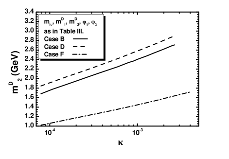
Figure 3: Contours in the $\kappa-m^{\rm D}_{2}$ plane yielding the central $Y_{B}$ in Eq. (81) consistently with the inflationary requirements for $\kappa_{T}=0.005$, $\lambda=0.05$, $M_{T}=3\times 10^{16}~{}{\mbox{\rm GeV}}$, $k_{8S}=1$, $k_{10S}=-1$, $k_{12S}=0$, $n_{\rm s}=0.96$, and the values of $m_{i\nu}$, $m^{\rm D}_{1}$, $m^{\rm D}_{3}$, $\varphi_{1}$, and $\varphi_{2}$ which correspond to the cases B (solid line), D (dashed line), and F (dot-dashed line) of Table 3.

The resulting contours in the $\kappa-m^{\rm D}_{2}$ plane are presented in Fig. 3 – since the range of $Y_{B}$ in Eq. (81) is very narrow, the $95\%$ c.l. width of these contours is negligible. The convention adopted for these lines is also described in the figure. In particular, we use solid, dashed, or dot-dashed line for $m_{[\nu}i]$, $m^{\rm D}_{1}$, $m^{\rm D}_{3}$, $\varphi_{1}$, and $\varphi_{2}$ corresponding to the cases B, D, or F of Table 3 respectively. The lower limit on these lines comes from the violation of Eqs. (21) and (23) – as in Figs. 2($b_{1}$) and ($b_{2}$). At the other end, these lines terminate at the values of $m^{\rm D}_{2}$ beyond which the second inequality in Eq. (75) is violated and, therefore, washout effects start becoming significant. At these upper termination points of the contours, we obtain $T_{\rm rh}\simeq 2\times 10^{9}~{}{\mbox{\rm GeV}}$ or $Y_{\widetilde{G}}\simeq 4\times 10^{-13}$ and so we expect that the constraint of Eq. (82) will cut any possible extension of the these curves beyond these termination points that could survive the possible washout of $Y_{L}$. Along the depicted contours, we obtain $8\times 10^{-2}\lesssim\kappa/10^{-3}\lesssim 4$, $2.3\lesssim m_{\rm I-}/10^{12}{\mbox{\rm GeV}}\lesssim 200$, whereas the naturalness parameter of the hilltop FHI $\Delta_{\rm m*}=0.05-0.27$. Also the resulting $M_{{[}\nu^{c}}2]$’s vary in the range $(4-19)\times 10^{10}~{}{\mbox{\rm GeV}}$ and $M_{{[}\nu^{c}}1]$ remains close to $(1-2)\times 10^{10}~{}{\mbox{\rm GeV}}$. The values of $y_{2L}$, $y^{\prime}_{2L}$ selected in Table 3 for the cases B, D, and F change also along the displayed curves of Fig. 3, without any essential modification though as regards their general features.

VII Conclusions

We constructed a SUSY GUT model based on the left-right symmetric gauge group $G_{\rm LR}$, which supports FHI followed by successful reheating and non-thermal leptogenesis. The lepton-number asymmetry is generated via the decay of the right-handed neutrinos $\nu^{c}_{i}$ which emerge from the decay of the inflaton system during the reheating process. It is important that any possible washout of the produced lepton asymmetry can be avoided. Our proposal is tied to the addition of two pairs of superfields (one pair consisting of bidoublets under ${\rm SU(2)_{L}}\times{\rm SU(2)_{R}}$ and another consisting of triplets under ${\rm SU(2)_{R}}$) – see Table I –, which naturally leads to an adequately strong violation of the asymptotic partial YU predicted by the simplest left-right symmetric model of Ref. vlachos . Confining our discussion to the trivial inflationary path, we found that the extra triplets play a crucial role (i) in the inflationary scenario causing extra radiative corrections along the inflationary path, and (ii) in the reheating process assisting us in obtaining an acceptably low reheat temperature.

We expanded the Kähler potential – see Eq. (30) – up to twelfth order in powers of the various fields and selected a convenient choice of signs which ensures that the parameters of the superpotential of our model assume values compatible with the requirement of gauge coupling constant unification within MSSM with the inflationary potential $V_{\rm HI}$ remaining bounded below at least up to the Planck scale $m_{\rm P}$. The FHI reproduces the current data on the amplitude $A_{\rm s}$ of the power spectrum of the curvature perturbation and the scalar spectral index $n_{\rm s}$ within the power-law $\Lambda$CDM cosmological model and generates the number of e-foldings required for the resolution of the horizon and flatness problems of the standard big bang cosmological model.

Imposing additional constraints from the BAU, the (unstable) gravitino abundance, and the neutrino oscillation parameters, we concluded that, for the central value of $n_{\rm s}$, $\kappa\simeq 8\times 10^{-5}-0.004$ and $m^{\rm D}_{1}\gtrsim 0.1~{}{\mbox{\rm GeV}}$ with the remaining parameters of the superpotential of our model taking more or less natural values, whereas the naturalness parameter for the hilltop FHI $\Delta_{\rm m*}\simeq 0.05-0.27$. It is gratifying that our model exhibits solutions with the inflaton system decaying exclusively into the lightest of the right-handed neutrinos $\nu^{c}_{i}$. These solutions are the most promising from the perspective of the gravitino constraint.

Appendix A Reheating Process, Lepton Asymmetry and Gravitino Abundance

In this Appendix, we present a numerical description of the post-inflationary evolution of the various energy and number densities involved in our scenario of non-thermal leptogenesis.

In particular, the energy densities $\rho_{+}$ and $\rho_{-}$ of the ${\rm I}_{+}$ and ${\rm I}_{-}$ subsystems respectively – see the definition of these subsystems right after Eq. (58) –, the energy density $\rho_{\rm R}$ of the produced radiation, and the number densities $n_{L}$ of the leptons and $n_{\widetilde{G}}$ of the $\widetilde{G}$’s satisfy the following Boltzmann equations – cf. Refs. gpp ; kohri :

$$\dot{\rho}_{+}+3H\rho_{+}+\Gamma_{\rm I+}\rho_{+}=0,$$ (84a)

$$\dot{\rho}_{-}+3H\rho_{-}+\Gamma_{\rm I-}\rho_{-}=0,$$ (84b)

$$\dot{\rho}_{\rm R}+4H\rho_{\rm R}-\mbox{$\sum_{r=\pm}$}\Gamma_{{\rm I}r}\rho_{r}=0,$$ (84c)

$$\dot{n}_{L}+3Hn_{L}-\mbox{$\sum_{r=\pm}$}2\varepsilon_{Lr}\Gamma_{{\rm I}r}n_{r}=0,$$ (84d)

$$\dot{n}_{\widetilde{G}}+3Hn_{\widetilde{G}}-C_{\widetilde{G}}\left(n^{\rm eq}\right)^{2}=0.$$ (84e)

Here the overdot denotes derivation with respect to the cosmic time $t$, $\varepsilon_{Lr}=\sum_{i}{\Gamma_{[}{\rm I}_{r}\rightarrow\nu^{c}_{i}]\varepsilon_{i}/\Gamma_{[}{\rm I}r]}$, and $n_{r}=\rho_{r}/m_{{\rm I}r}$. Also, $n^{\rm eq}={\zeta(3)T^{3}/\pi^{2}}$ is the equilibrium number density of each bosonic relativistic species, $C_{\widetilde{G}}$ is a collision term for $\widetilde{G}$ production which, in the limit of massless MSSM gauginos, turns out to be kohri ; brand

$$C_{\widetilde{G}}=\frac{3\pi}{16\zeta(3)m_{\rm P}^{2}}\sum_{i=1}^{3}c_{i}g_{i}^{2}\ln\left(\frac{k_{i}}{g_{i}}\right),$$ (85)

where $(c_{i})=(33/5,27,72)$, $g_{i}$ are the gauge coupling constants of the MSSM, and $(k_{i})=(1.634,1.312,1.271)$. Finally, the Hubble expansion parameter $H$ during this period is given by

$$H=\frac{1}{\sqrt{3}m_{\rm P}}\left(m_{{\widetilde{G}}}n_{{\widetilde{G}}}+\rho_{-}+\rho_{+}+\rho_{\rm R}\right)^{1/2}.$$ (86)

Clearly, in the limit of massless MSSM gauginos, the resulting $n_{\widetilde{G}}$ is practically $m_{\widetilde{G}}$-independent. The temperature $T$ and the entropy density $s$ are found from the relations

$$\rho_{\rm R}=\frac{\pi^{2}}{30}g_{*}T^{4}~{}\mbox{and}~{}s=\frac{2\pi^{2}}{45}g_{*}T^{3}.$$ (87)

The system of Eqs. (84a)-(84e) is solved under the following initial conditions:

$$\rho_{+}(0)=\rho_{-}(0)=V_{\rm HI0}/2$$ (88a)

and

$$\rho_{\rm R}(0)=n_{\widetilde{G}}(0)=n_{L}(0)=0,$$ (88b)

where we assumed that the inflationary energy density is equally distributed between the oscillatory subsystems ${\rm I}_{+}$ and ${\rm I}_{-}$. This is a reasonable assumption since the damped oscillations of I₊ and I_- commence immediately after the termination of FHI as a consequence of the fact that $m_{\rm I+}$ and $m_{\rm I-}\gg H_{\rm I0}\equiv\sqrt{V_{\rm HI0}}/\sqrt{3}m_{\rm P}$, the inflationary Hubble parameter.

In Fig. 4, we illustrate the cosmological evolution of the quantities $\log\rho_{+}$ (dotted gray line), $\log\rho_{-}$ (dashed gray line), $\log\rho_{\rm R}$ (gray line), $\log|Y_{L}|$ (black solid line), and $\log|Y_{\widetilde{G}}|$ (black dashed line) as functions of $\log T$ for the values of the parameters given in the first column of Table 3 (case A). In particular, these parameters yield $m_{\rm I+}=2.5\times 10^{16}~{}{\mbox{\rm GeV}}$ and $\Gamma_{[}{\rm I}+]=4.1\times 10^{10}~{}{\mbox{\rm GeV}}$ for the ${\rm I}_{+}$ subsystem, whereas $m_{\rm I-}=2.9\times 10^{13}~{}{\mbox{\rm GeV}}$ and $\Gamma_{[}{\rm I}-]=0.62~{}{\mbox{\rm GeV}}$ for the ${\rm I}_{-}$ subsystem. Since $H_{\rm I0}\simeq 1.65\times 10^{11}~{}{\mbox{\rm GeV}}\ll m_{\rm I+}$ and $m_{\rm I-}$, we verify that the phase of the oscillations of ${\rm I}_{+}$ and ${\rm I}_{-}$ starts immediately after the end of FHI.

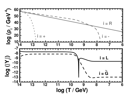
Figure 4: The evolution of the quantities $\log\rho_{i}$ with $i=+$ (gray dotted line), $i=-$ (gray dashed line), $i={\rm R}$ (gray line), $\log|Y_{L}|$ (black solid line), and $\log|Y_{\widetilde{G}}|$ (black dashed line) as functions of $\log T$ for the values of the parameters in the case A of Table 3.

From Fig. 4, we observe that FHI is followed by an extended matter dominated era, where we have initially the dominance of the oscillating and decaying ${\rm I}_{+}$ and ${\rm I}_{-}$ subsystems. Due to the strong hierarchy between $\Gamma_{[}\rm I+]$ and $\Gamma_{[}\rm I-]$, the decay of ${\rm I}_{+}$ occurs very early at $T=T_{+}\simeq 7.2\times 10^{13}~{}{\mbox{\rm GeV}}$ – this temperature corresponds to the intersection of the $\rho_{+}$ and $\rho_{\rm R}$ lines in Fig. 4. An approximate estimate of this temperature can be obtained from Eq. (59) by replacing $\Gamma_{{\rm I}-}$ with $\Gamma_{{\rm I}+}$. This estimate is about $8.8\times 10^{13}~{}{\mbox{\rm GeV}}$, which is quite close to the value of $T_{+}$ found numerically. After the ${\rm I}_{+}$ decay, the ${\rm I}_{-}$ subsystem continues its oscillations until $\rho_{-}$ meets $\rho_{\rm R}$ at $T_{\rm rh}=3.5\times 10^{8}~{}{\mbox{\rm GeV}}$. This numerical result is in excellent agreement with the estimate obtained by using Eq. (59), which is listed in the column A of Table 3. After reheating, the universe enters a conventional radiation dominated era. Therefore, although our scenario involves two oscillatory systems, ${\rm I}_{+}$ and ${\rm I}_{-}$, the final $T_{\rm rh}$ can be accurately computed by Eq. (59) thanks to the strong hierarchy encountered between $\Gamma_{{\rm I}+}$ and $\Gamma_{{\rm I}-}$.

In Fig. 4, we also depict the cosmological evolution of the absolute values of the lepton abundance $Y_{L}=n_{L}/s$ and the gravitino abundance $Y_{\widetilde{G}}=n_{{\widetilde{G}}}/s$. We see that $|Y_{L}|$ and $|Y_{\widetilde{G}}|$, immediately after the decay of the ${\rm I}_{+}$ subsystem, reach constant values equal to $3\times 10^{-9}$ and $2.6\times 10^{-8}$ respectively. However, they are later strongly diluted due to the entropy release during the subsequent decay of the ${\rm I}_{-}$ subsystem. The lepton abundance $Y_{L}$ at $T=T_{+}$ originates from the lepton asymmetry $2\varepsilon_{L+}$ generated by the decay of one ${\rm I}_{+}$ inflaton – $\varepsilon_{L+}$ is defined just below Eq. (84e). However, the subsequent decay of the ${\rm I}_{-}$ subsystem gives rise to a new lepton asymmetry $2\varepsilon_{L-}$ per decaying inflaton. Note that the sign of this new asymmetry, which survive for $T<T_{\rm rh}$, is opposite to the sign of the earlier one which was diluted. As a consequence of this cosmological evolution, the present values of both $Y_{L}$ and $Y_{\widetilde{G}}$ are generated close to $T\simeq T_{\rm rh}$. Numerically, we find that $Y_{L}=-2\times 10^{-10}$ and $Y_{\widetilde{G}}=10^{-13}$, which are in good agreement with the values obtained by using Eqs. (60b) and (61) in the case A of Table 3 – note that the corresponding $Y_{B}$ turns out to be $7.6\times 10^{-11}$. Therefore, we see that Eqs. (60b) and (61), despite their simplicity, give a very accurate determination of $Y_{B}$ and $Y_{\widetilde{G}}$ in our set-up.

References

- (1) E.J. Copeland, A.R. Liddle, D.H. Lyth, E.D. Stewart, and D. Wands, Phys. Rev. D 49, 6410 (1994).
- (2) G.R. Dvali, Q. Shafi, and R.K. Schaefer, Phys. Rev. Lett. 73, 1886 (1994).
- (3) G. Lazarides, Lect. Notes Phys. 592, 351 (2002); J. Phys. Conf. Ser. 53, 528 (2006).
- (4) G.R. Dvali, G. Lazarides, and Q. Shafi, Phys. Lett. B 424, 259 (1998).
- (5) G. Lazarides and Q. Shafi, Phys. Rev. D 58, 071702 (1998).
- (6) G. Lazarides and C. Pallis, Phys. Rev. D 82, 063535 (2010); C. Pallis, PoS (CORFU2011), 028 (2011).
- (7) R. Peccei and H. Quinn, Phys. Rev. Lett. 38, 1440 (1977); S. Weinberg, ibid. 40, 223 (1978); F. Wilczek, ibid. 40, 279 (1978).
- (8) G. Lazarides and Q. Shafi, Phys. Lett. B 258, 305 (1991); G. Lazarides, R.K. Schaefer, and Q. Shafi, Phys. Rev. D 56, 1324 (1997); G. Lazarides, Q. Shafi, and N.D. Vlachos, Phys. Lett. B 427, 53 (1998).
- (9) G.’t Hooft, Nucl. Phys. B79, 276 (1974); A.M. Polyakov, JETP Lett. 20, 194 (1974); J.P. Preskill, Phys. Rev. Lett. 43, 1365 (1979); G. Lazarides, Q. Shafi, and W.P. Trower, ibid. 49, 1756 (1982).
- (10) T.W.B. Kibble, J. Phys. A 9, 1387 (1976); G. Lazarides, Q. Shafi, and T.F. Walsh, Nucl. Phys. B195, 157 (1982); T.W.B. Kibble, G. Lazarides, and Q. Shafi, Phys. Lett. B 113, 237 (1982).
- (11) C. Pallis, “High Energy Physics Research Advances”, edited by T.P. Harrison and R.N. Gonzales (Nova Science Publishers Inc., New York, 2008) [arXiv:0710.3074]; R. Armillis and C. Pallis, “Recent Advances in Cosmology”, edited by A. Travena and B. Soren (Nova Science Publishers Inc., New York, 2013) [arXiv:1211.4011].
- (12) M. ur Rehman, Q. Shafi, and J.R. Wickman, Phys. Rev. D 83, 067304 (2011).
- (13) P.A.R. Ade et al. [Planck Collaboration], arXiv:1303.50 82.
- (14) E. Komatsu et al.[WMAP Collaboration], Astrophys. J. Suppl. 192, 18 (2011); G. Hinshaw et al.[WMAP Collaboration], arXiv:1212.5226.
- (15) G. Lazarides and N.D. Vlachos, Phys. Lett. B 459, 482 (1999).
- (16) R. Jeannerot, S. Khalil, and G. Lazarides, J. High Energy Phys. 07, 069 (2002).
- (17) G. Lazarides and A. Vamvasakis, Phys. Rev. D 76, 083507 (2007).
- (18) G. Lazarides and A. Vamvasakis, Phys. Rev. D 76, 123514 (2007); G. Lazarides, arXiv:1006.3636.
- (19) G. Lazarides, I.N.R. Peddie, and A. Vamvasakis, Phys. Rev. D 78, 043518 (2008).
- (20) M.Yu. Khlopov and A.D. Linde, Phys. Lett. B 138, 265 (1984); J. Ellis, J.E. Kim, and D.V. Nanopoulos, ibid. 145, 181 (1984); I.V. Falomkin, D.B. Pontecorvo, M.G. Sapozhnikov, M.Yu. Khlopov, F. Balestra, and G. Piragino, Sov. J. Nucl. Phys. 39, 626 (1984); J.R. Ellis, D.V. Nanopoulos, and S. Sarkar, Nucl. Phys. B259, 175 (1985); J.R. Ellis, G.B. Gelmini, J.L. López, D.V. Nanopoulos, and S. Sarkar, ibid. B373, 399 (1992).
- (21) R.H. Cyburt, J.R. Ellis, B.D. Fields, and K.A. Olive, Phys. Rev. D 67, 103521 (2003); M. Kawasaki, K. Kohri, and T. Moroi, Phys. Lett. B 625, 7 (2005); Phys. Rev. D 71, 083502 (2005); J.R. Ellis, K.A. Olive, and E. Vangioni, Phys. Lett. B 619, 30 (2005).
- (22) L. Boubekeur and D. Lyth, J. Cosmol. Astropart. Phys. 07, 010 (2005); K. Kohri, C.M. Lin, and D.H. Lyth, ibid. 12, 004 (2007); C.M. Lin and K. Cheung, ibid. 03, 012 (2009).
- (23) B. Garbrecht, C. Pallis, and A. Pilaftsis, J. High Energy Phys. 12, 038 (2006).
- (24) G. Lazarides, R. Ruiz de Austri, and R. Trotta, Phys. Rev. D 70, 123527 (2004).
- (25) G. Lazarides and C. Panagiotakopoulos, Phys. Rev. D 52, R559 (1995); G. Lazarides, C. Panagiotakopoulos, and N.D. Vlachos, ibid. 54, 1369 (1996); R. Jeannerot, S. Khalil, and G. Lazarides, Phys. Lett. B 506, 344 (2001); M. ur Rehman and Q. Shafi, Phys. Rev. D 86, 027301 (2012); S. Khalil, Q. Shafi, and A. Sil, ibid. 86, 073004 (2012).
- (26) R. Jeannerot, S. Khalil, G. Lazarides, and Q. Shafi, J. High Energy Phys. 10, 012 (2000); S. Khalil, M. ur Rehman, Q. Shafi, and E.A. Zaakouk, Phys. Rev. D 83, 063522 (2011); M. Civiletti, M. ur Rehman, Q. Shafi, and J.R. Wickman, ibid. 84, 103505 (2011).
- (27) J. Rocher and M. Sakellariadou, J. Cosmol. Astropart. Phys. 03, 004 (2005); R. Jeannerot and M. Postma, J. High Energy Phys. 05, 071 (2005).
- (28) G. Lazarides, C. Panagiotakopoulos, and Q. Shafi, Phys. Rev. Lett. 56, 432 (1986).
- (29) N. Ganoulis, G. Lazarides, and Q. Shafi, Nucl. Phys. B323, 374 (1989); G. Lazarides and Q. Shafi, ibid. B329, 182 (1990).
- (30) N. Karagiannakis, G. Lazarides, and C. Pallis, arXiv: 1305.2574.
- (31) G. Lazarides and C. Panagiotakopoulos, Phys. Lett. B 337, 90 (1994); S. Khalil, G. Lazarides, and C. Pallis, ibid. 508, 327 (2001).
- (32) N. Karagiannakis, G. Lazarides, and C. Pallis, Phys. Rev. D 87, 055001 (2013).
- (33) S. Antusch, L. Calibbi, V. Maurer, M. Monaco, and M. Spinrath, Phys. Rev. D 85, 035025 (2012); J. High Energy Phys. 01, 187 (2013).
- (34) M.E. Gómez, G. Lazarides, and C. Pallis, Nucl. Phys. B638, 165 (2002); G. Lazarides and C. Pallis, hep-ph/0404266; hep-ph/0406081.
- (35) M.E. Gómez, G. Lazarides, and C. Pallis, Phys. Rev. D 67, 097701 (2003).
- (36) N. Karagiannakis, G. Lazarides, and C. Pallis, Phys. Lett. B 704, 43 (2011); PoS (CORFU2011), 023 (2011).
- (37) N. Karagiannakis, G. Lazarides, and C. Pallis, J. Phys. Conf. Ser. 384, 012012 (2012).
- (38) S. Coleman and E. Weinberg, Phys. Rev. D 7, 1888 (1973).
- (39) D.H. Lyth and A. Riotto, Phys. Rept. 314, 1 (1999); A. Mazumdar and J. Rocher, ibid. 497, 85 (2011).
- (40) M. Bastero-Gil, S.F. King, and Q. Shafi, Phys. Lett. B 651, 345 (2007); M. ur Rehman, V.N. Şenoğuz, and Q. Shafi, Phys. Rev. D 75, 043522 (2007).
- (41) D.V. Forero, M. Tortola, and J.W.F. Valle, Phys. Rev. D 86, 073012 (2012).
- (42) G.L. Fogli, E. Lisi, A. Marrone, D. Montanino, A. Palazzo, and A.M. Rotunno, Phys. Rev. D 86, 013012 (2012).
- (43) T. Dent, G. Lazarides, and R. Ruiz de Austri, Phys. Rev. D 72, 043502 (2005).
- (44) M. Endo, M. Kawasaki, F. Takahashi, and T.T. Yanagida, Phys. Lett. B 642, 518 (2006); M. Endo, F. Takahashi, and T.T. Yanagida, Phys. Rev. D 76, 083509 (2007).
- (45) C. Pallis, Nucl. Phys. B751, 129 (2006).
- (46) K. Hamaguchi, hep-ph/0212305; W. Buchmuller, R.D. Peccei, and T. Yanagida, Ann. Rev. Nucl. Part. Sci. 55, 311 (2005).
- (47) L.E. Ibáñez and F. Quevedo, Phys. Lett. B 283, 261 (1992).
- (48) V.N. Şenoğuz, Phys. Rev. D 76, 013005 (2007).
- (49) M. Fukugita and T. Yanagida, Phys. Rev. D 42, 1285 (1990).
- (50) P.A.R. Ade et al. [Planck Collaboration], arXiv:1303.50 76.
- (51) K. Dimopoulos, G. Lazarides, D. Lyth, and R. Ruiz de Austri, J. High Energy Phys. 05, 057 (2003).
- (52) G. Lazarides and A. Mariano, in preparation.
- (53) H. Baer, S. Kraml, A. Lessa, and S. Sekmen, J. Cosmol. Astropart. Phys. 04, 039 (2011).
- (54) M. Kawasaki, K. Nakayama, and M. Senami, J. Cosmol. Astropart. Phys. 03, 009 (2008).
- (55) G. Lazarides, Lect. Notes Phys. 720, 3 (2007).
- (56) K.J. Bae, E.J. Chun, and S.H. Im, J. Cosmol. Astropart. Phys. 03, 013 (2012).
- (57) M. Flanz, E.A. Paschos, and U. Sarkar, Phys. Lett. B 345, 248 (1995); 382, 447(E) (1996); L. Covi, E. Roulet, and F. Vissani, ibid. 384, 169 (1996); M. Flanz, E.A. Paschos, U. Sarkar, and J. Weiss, ibid. 389, 693 (1996).
- (58) G.C. Branco, R. González Felipe, F.R. Joaquim, and M.N. Rebelo, Nucl. Phys. B640, 202 (2002); E.K. Akhmedov, M. Frigerio, and A.Y. Smirnov, J. High Energy Phys. 09, 021 (2003); S. Pascoli, S.T. Petcov, and W. Rodejohann, Phys. Rev. D 68, 093007 (2003).
- (59) J. Kopp, Int. J. Mod. Phys. C 19, 523 (2008).
- (60) G. Aad et al. [ATLAS Collaboration], Phys. Lett. B 716, 1 (2012); S. Chatrchyan et al. [CMS Collaboration], Phys. Lett. B 716, 30 (2012).
- (61) S. Antusch and M. Spinrath, Phys. Rev. D 78, 075020 (2008).
- (62) S. Antusch, J. Kersten, M. Lindner, and M. Ratz, Nucl. Phys. B674, 401 (2003).
- (63) M. Bolz, A. Brandenburg, and W. Buchmüller, Nucl. Phys. B606, 518 (2001); B790, 336(E) (2008); J. Pradler and F.D. Steffen, Phys. Rev. D 75, 023509 (2007).