Orbital Parameters for the Two Young Binaries VSB 111 and VSB 126

Abstract

We report orbital parameters for two low-mass, pre-main sequence, double-lined spectroscopic binaries VSB 111 and VSB 126. These systems were originally identified as single-lined on the basis of visible-light observations. We obtained high-resolution, infrared spectra with the 10-m Keck II telescope, detected absorption lines of the secondary stars, and measured radial velocities of both components in the systems. The visible light spectra were obtained on the 1.5-m Wyeth reflector at the Oak Ridge Observatory, the 1.5-m Tillinghast reflector at the F. L. Whipple Observatory, and the 4.5-m equivalent Multiple Mirror Telescope. The combination of our visible and infrared observations of VSB 111 leads to a period of 902.1$\pm$0.9 days, an eccentricity of 0.788$\pm$0.008, and a mass ratio of 0.52$\pm$0.05. VSB 126 has a period of 12.9244$\pm$0.0002 days, an eccentricity of 0.18$\pm$0.02, and a mass ratio of 0.29$\pm$0.02. Visible-light photometry, using the 0.8-m telescope at Lowell Observatory, provided rotation periods for the primary stars in both systems, 3.74$\pm$0.02 days for VSB 111 and 5.71$\pm$0.07 days for VSB 126. Both binaries are located in the young, active star-forming cluster NGC 2264 at a distance of $\sim$800 pc. The difference in the center-of-mass velocities of the two systems is consistent with the radial velocity gradient seen across NGC 2264. To test the evolutionary models for accuracy and consistency, we compare the stellar properties derived from several sets of theoretical calculations for pre-main sequence evolution with our dynamical results.

1 Introduction

A binary star provides one of the few ways to directly measure stellar masses. The mass is the most important property of a star and determines its basic structure and properties, as well as the duration of stages of evolution throughout its lifetime. A double-lined spectroscopic binary (SB2) enables the orbit to be solved from spectroscopically-determined radial velocities (RVs), yielding the orbital elements (except $i$) and mass ratio, $q$, for the component stars. Component masses may be found if the inclination of an SB2 can be measured in the case of an eclipsing binary system ($i$=90$\,{}^{\circ}$) or a resolved visual binary.

The work presented here is part of a long-term program to measure young SB2 mass ratios and eventually component masses, $M{{}_{1}}$ and $M{{}_{2}}$ (Prato et al. 2002; Schaefer et al. 2012). Such results will be facilitated with the advent of high-precision astrometric missions such as GAIA. Ultimately, a large sample of precise, dynamical masses will help to anchor models of pre-main sequence (PMS) evolution to a solid observational basis, particularly for systems with stellar mass $<$1 M_⊙ (e.g., Hillenbrand & White 2004; Simon 2008). Furthermore, precise measurements of the mass-ratio distribution provide critical input for theories of binary star formation (Bate 2009). Our present goal is to build up a large sample of young star mass ratios.

Vasilevskis, Sanders, & Balz (1965) included VSB 111 (V810 Mon) and VSB 126 (2MASS J06410777+0944030) in their study. Since then, several papers adopted the VSB acronym; therefore, we use those names throughout the paper. VSB 111 and VSB 126 are located in the young cluster NGC 2264. This cluster is an active region of star formation, with subclusters of suspected members spread across several parsecs. Dahm (2008) published a summary of the papers on NGC 2264. There are numerous estimates of the distance to NGC 2264, ranging from 700 pc (Feldbrugge & van Genderen 1991) to 950 pc (Pérez et al. 1987). We adopted a distance of 800 pc from Walker (1956) because it was a median value within the estimated distances published in Dahm (2008). We adopted an uncertainty of $\pm$100 pc to account for the large spread of published distances. Additionally, there is a large age range cited in the literature. Estimates for the age of the cluster range from 0.1 Myr (Flaccomio et al. 1999; Rebull et al. 2002) to 10.0 Myr (Flaccomio et al. 1999), but $\sim$3.0 Myr is common (Walker 1956; Mendoza & Gómez 1980; Feldbrugge & van Genderen 1991; Sung et al. 2004; Ramirez et al. 2004; Flaccomio et al. 2006). This is not particularly surprising, however, as the ages of stars in young clusters typically appear to span a range of millions and even tens of millions of years (e.g., Hillenbrand 1997).

Haisch et al. (2001) observed that about half of the stars within clusters lose their disks in approximately 3 Myr. Mathieu (1994) lists the H$\alpha$ equivalent widths for VSB 111 as -0.3 Å and VSB 126 as -1.9 Å, indicating a lack of any appreciable gas accretion in these systems. WISE and Spitzer data show no indication of warm dust in VSB 111 and VSB 126. We therefore believe they are diskless. The basic properties of the systems are listed in Table 1.

Mathieu (1994) originally derived single-lined spectroscopic (SB1) orbital solutions for VSB 111 and VSB 126. Given his mass functions for the systems, we knew a priori that the minimum mass ratios were both likely to be small. When a low mass ratio binary system is observed in visible light, the primary star’s spectrum dominates the faint secondary signal because of the low flux ratio. Observing in the infrared (IR) allows for detection of the secondary component and thus solution of the system as an SB2 because the flux ratio is more favorable in the long-wavelength Rayleigh-Jeans regime. This approach was demonstrated in Prato (1998), Mazeh et al. (2002), Prato et al. (2002), and Mazeh et al. (2003). Observing PMS binaries in the IR can also be advantageous for young stars obscured in dusty star forming regions (SFRs).

In this paper we contribute dynamical mass-ratio measurements for two young binaries, one short-period (several days) and one long-period (few years), to the as yet relatively small sample of $\sim$50 PMS SB2s. Furthermore, our results provide improved orbital parameters for both binaries. Based on the stellar characteristics and light curves measured as part of this program, we also estimated the inclinations of the binary orbital planes and the stellar rotation axes. In §2 we describe our observations and data reduction. In §3 we provide our analysis and results. A discussion appears in §4 and §5 summarizes our findings.

2 Observations and Data Reduction

2.1 Visible Light Spectroscopy

Visible light spectroscopic observations of VSB 111 and VSB 126 were carried out at the Harvard-Smithsonian Center for Astrophysics (CfA) using three different telescopes equipped with nearly identical echelle spectrographs: the 1.5-m Wyeth reflector at the Oak Ridge Observatory (Harvard, Massachusetts), the 1.5-m Tillinghast reflector at the F. L. Whipple Observatory (Mount Hopkins, Arizona), and the 4.5-m equivalent Multiple Mirror Telescope (also on Mount Hopkins), prior to its conversion to a monolithic 6.5 mirror. A single echelle order 45 Å wide and centered near 5190 Å (including the Mg I b triplet) was recorded with intensified photon-counting Reticon detectors at a resolving power of $\lambda/\Delta\lambda=35,\!000$. We collected 69 spectra for VSB 111 between 1984 January and 1996 January, with signal-to-noise ratios between 8–20 per resolution element of 8.5 km s^-1. For VSB 126 we collected a total of 30 spectra from 1984 March to 1992 February, at signal to noise ratios of 5 to 11 per resolution element. These data are largely the same as those on which the results of Mathieu (1994) are based. The details of the observations are provided here for the first time. The specific dates of observation appear in the first column of Tables 2 and 3 . Spectra were reduced using standard IRAF procedures for echelle data (e.g., Torres et al. 1997).

2.2 Infrared Spectroscopy

VSB 111 and VSB 126 were observed in the IR with the Keck II 10-m telescope on Mauna Kea. The observations for VSB 111 and VSB 126 were made between 2001 December and 2012 January (Tables 4 and 5). The Keck facility near-IR spectrograph, NIRSPEC, was used to obtain $H$-band data at a central wavelength of $\sim$1.555 $\mu$m (McLean et al. 1998; 2000). NIRSPEC employs a 1024 x 1024 ALADDIN InSb array detector. The $0\farcs 288$ (2 pixel) x $24^{\prime\prime}$ slit yielded a resolution of R=30,000. The slit viewing camera, SCAM, which uses a 256 x 256 HgCdTe detector with 0$\farcs$18 pixels, facilitated source acquisition and guiding. For VSB 111, integration times for the individual frames were 240 s or 300 s; two to eight frames were taken on each observing date. For VSB 126, integration times for the individual frames were 300 s or 360 s; six to fourteen frames were taken on each visit. For both systems, the signal to noise ratio was always $>$100 and typically 200 or higher. Background subtraction was achieved between consecutive spectra by nodding the telescope $12^{\prime\prime}$ to dither the target between two positions on the slit and using an A-B-B-A pattern of observation.

Our $H$-band setting (echelle$=63\fdg 04$, cross-disperser$=36\fdg 3$) has a central wavelength of $\sim$1.555 $\mu$m, which corresponds to order 49 (1.545$-$1.567 $\mu$m) for NIRSPEC. We focused on order 49 because it is free of telluric absorption lines and contains well-spaced OH emission lines. De-excitation of the hydroxyl molecule (OH) in the Earth’s atmosphere produces these emission lines; they are distributed throughout order 49 and were used to calibrate the wavelength zero-point and dispersion (Rousselot et al. 2000). Order 49 is also rich in atomic and molecular species in the stellar photospheres that allow us to identify spectral features of both warm and cool stars.

NIRSPEC’s optics optimize the throughput of photons but the resulting spectra do not fall along uniform rows; the light falls in curved swaths. Therefore, we needed to rectify the data spatially and spectrally. For all data reduction we used the REDSPEC software package, written at UCLA by S. Kim, L. Prato, and I. McLean, and created specifically for the analysis of NIRSPEC data. The lack of terrestrial absorption lines in order 49 eliminates the need to divide by telluric standard star spectra. Median images of 10 flat and 10 dark files were used to create a master flat and dark in order to correct for effects from the detector.

The REDSPEC module spatmap was used to remap the raw images onto a uniform interval coordinate system in the spatial (cross-dispersion) direction by adding two nodded frames together and fitting a $3^{rd}$ order polynomial to each spectral trace. The specmap module was used to remap the raw images onto uniform interval coordinate system in the dispersion direction. A $2^{nd}$ order polynomial was fit to each OH line to identify the approximately vertical trace. Then, a $2^{nd}$ order polynomial fit in the dispersion direction was made to these wavelength locations for each row around the spectral trace. The final step of REDSPEC was to divide by the dark-subtracted master flat, remove any bad pixels and fringing, and clip out and sum the rows containing the rectified spectra. All spectra were corrected for heliocentric motion and the Earth’s rotation using JSkyCalc¹ and are shown in Figures 1 and 2 for VSB 111 and VSB 126, respectively.

2.3 Visible Light Photometry

The photometric data were taken on twelve nights between 2012 September 14 and October 11 using the Lowell 0.8-m telescope in robotic mode. A total of 45 images were obtained for VSB 111 and 44 images for VSB 126. The CCD camera houses an e2v 2k$\times$2k chip providing a $15^{\prime}\times 15^{\prime}$ field. The image scale is $0\farcs 91$/pixel when binned 2$\times$2, as here. A median bias frame was produced every night from several dozen zero-integration time exposures. Twilight flats are scripted for each filter in use on a rotating schedule and taken when obtainable. Further details about the telescope and its conversion to robotic use can be found in Buie (2010). Pairs of 150 s exposures using a Johnson $V$ filter were taken at each visit to NGC 2264. These were observed among roughly a dozen other targets in the queue schedule whenever the field was at less than 2.0 airmasses. Since the observing was done near the beginning of the season, typically four visits (up to eight) were made to the field each night roughly a half hour to a full hour apart. The images were reduced with the commercial photometry package $Canopus$ (Warner 2011). The software includes a photometric catalogue with $BVRI$ data derived from 2MASS $JHK_{s}$ photometry (Warner 2007), as well as more traditional published $BVRI$ photometry, and Sloan $griz$ catalogues. These provide photometric zero-points and color indices ($\sim$0.03 mag) for the entire sky via on-chip differential photometry without the need to observe primary standards. $Canopus$ plots the run of instrumental magnitudes versus its internal photometric catalogue of all stars in the image. The averaged photometry from the two frames at each visit to the field was used for analysis.

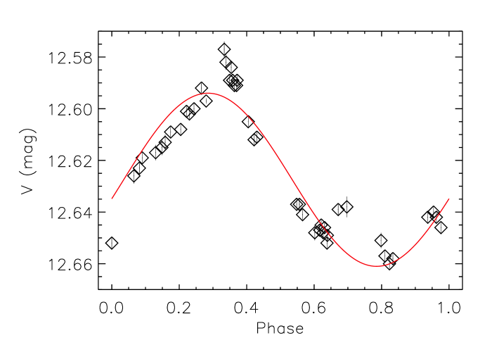
Figure 3: Magnitude versus phase for the primary component of VSB 111. The rotation period was determined to be 3.74$\pm$0.02 days. The magnitudes are binned in JD date to minimize the errors, shown as vertical bars. The red line is a weighted sinusoidal fit. The first image taken was used to phase the light curve and represents phase zero.

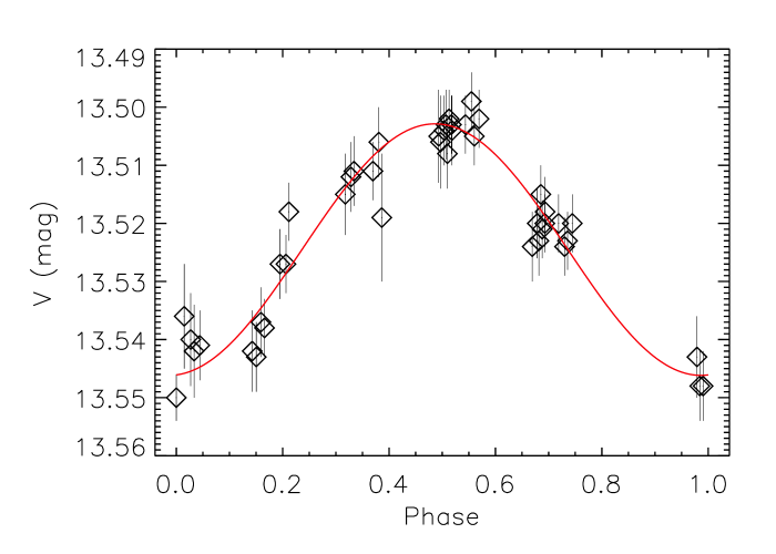
Figure 4: Same as Figure 3 for VSB 126. The rotation period was determined to be 5.71$\pm$0.07 days.

In the NGC 2264 region the majority of the brighter stars are identified or suspected variables. All five of the comparison stars we selected appear in the NSV catalogue or its supplements (Samus et al. 2012), and have been hitherto suspected to be variable with ranges of up to a half magnitude. Table 6 lists the coordinates and aliases of the comparison stars. The five comparison stars were chosen to be similar in color to the two binaries, which helps minimize errors in the photometry resulting from color terms and differential extinction. All five comparison stars are demonstrably constant at the half-percent level on the timescale of weeks. The reduced data for VSB 111 and VSB 126 are shown in Tables 7 and 8, respectively. The light curves for the primary star in each system are shown in Figures 3 and 4 for VSB 111 and VSB 126, respectively.

3 Analysis

3.1 Radial and Rotational Velocities

All our visible light CfA spectra appear single-lined. The templates that best match the spectra implicitly provide an estimate of the spectroscopic parameters of the primary stars. RVs were obtained by cross-correlation using the IRAF task XCSAO, with templates chosen from a large library of calculated spectra based on model atmospheres by R. L. Kurucz (Nordström et al. 1994; Latham et al. 2002). Of the four main parameters of these templates (effective temperature $T_{\rm eff}$, rotational velocity $v\sin i$, metallicity [Fe/H], and surface gravity $\log g$), the ones affecting the velocities the most are $T_{\rm eff}$ and $v\sin i$. Consequently, we held $\log g$ fixed at a value of 3.75 for both stars and assumed solar metallicity. The optimum $T_{\rm eff}$ and $v\sin i$ values were determined by running grids of cross-correlations seeking the maximum of the correlation coefficient, averaged over all exposures (Torres et al. 2002). We obtained $T_{\rm eff}$ = 5300$\pm$100$\,K$ and $v\sin i$ = 31$\pm$2 km s^-1 for VSB 111, and $T_{\rm eff}$ = 5460$\pm$100$\,K$ and $v\sin i$ = 13$\pm$2 km s^-1 for VSB 126.

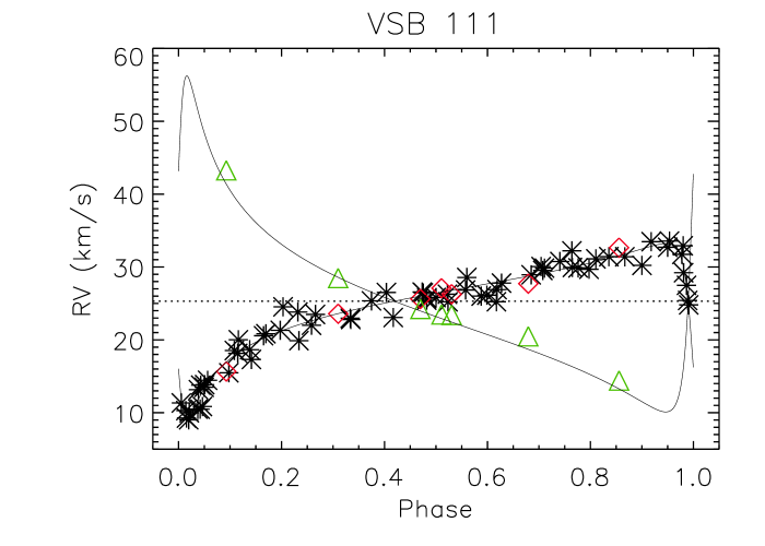
Figure 5: Radial velocity versus phase for VSB 111. Measured RVs for the primary in the optical are represented by black asterisks and in the IR by red diamonds. Measured RVs in the IR for the secondary are represented by green triangles. The dotted horizontal line is the center-of-mass velocity, $\gamma$. RV uncertainties are smaller than the plot symbol size and are given in Tables 2 and 4.

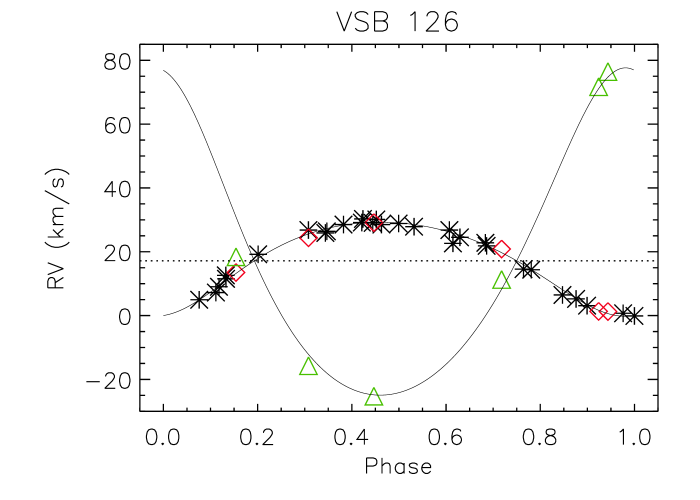
Figure 6: Same as Figure 5 for VSB 126. RV uncertainties are smaller than the plot symbol size and are given in Tables 3 and 5.

The stability of the zero-point of the velocity system (e.g., Latham 1992) was monitored by taking exposures of the dusk and dawn sky, and applying small run-to-run corrections as described by Latham (1992). The final heliocentric RVs including these corrections are listed in Tables 2 and 3. The RVs are plotted in Figures 5 and 6.

The individual RVs for the stars based on the IR data were determined by using a two-dimensional cross correlation algorithm developed at Lowell Observatory following Zucker & Mazeh (1994). The algorithm calculates the correlation of the target spectrum against two templates chosen to best match the primary and secondary components. Approximate spectral types for the VSB 111 and VSB 126 primary stars were known from visible light observations (Mathieu 1994). To begin the process of estimating secondary star spectral types, we used the mass function from Mathieu (1994) to find the minimum secondary mass by assuming a primary mass of 1.0 M_⊙ for both VSB 111 and VSB 126. We estimated the secondary spectral type from the minimum secondary mass using model data presented in Luhman et al. (2003; Figure 5). We then used template spectra with the corresponding spectral type for each component taken from the suite presented in Prato et al. (2002). The two templates were shifted in RV, combined, and correlated with the observed spectra for each epoch, enabling the identification of component RVs. The flux ratio, $\alpha$, was determined by maximizing the cross-correlation coefficient for each epoch and taking the average. Subsequently, the average flux ratios, 0.39$\pm$0.05 for VSB 111 and 0.13$\pm$0.05 for VSB 126, were held fixed and the RVs were redetermined. The rotational velocity, $v\sin i$, was measured by using a set of templates rotationally broadened to a range of $v\sin i$ values (e.g., Mace et al. 2012). We selected the $v\sin i$ that yielded the maximum correlation coefficient. Tables 4 and 5 show the UT dates and measured IR RVs of both components of VSB 111 and VSB 126, respectively. These RVs are plotted in Figures 5 and 6.

VSB 111 was found to best match a K0 template (BS 7368), with a $v\sin i$ of 30 km s^-1, and an M0 template (GL 763), with a $v\sin i$ of 15 km s^-1, for the primary and secondary components, respectively. VSB 126 was best fit with a K0 template (BS 7368), with a $v\sin i$ of 15 km s^-1, and an M4 template (GL 402), with a $v\sin i$ of 8 km s^-1, for the primary and secondary components, respectively. These spectral types, the equivalent values of $T_{\rm eff}$ from Luhman et al. (2003), and the $v\sin i$ values are all given in Table 9. Results from analysis of visible-light data are included for comparison. Conservative uncertainties of 5 km s^-1 are estimated for the IR $v\sin i$ values based on visual inspection of the spectra and comparison with standard star spectra convolved with different rotation kernels.

The uncertainties in the IR RVs for both VSB 111 and VSB 126 were initially set at 1.0 km s^-1 for the primary and 2.0 km s^-1 for the secondary (Prato et al. 2002). The uncertainties in the visible-light RVs for VSB 111 and VSB 126 were estimated by first using the internal errors of the RVs as initial guesses. After finding the best orbital fit (§3.2) for the single-lined data, we used the $\chi^{2}$ per degree of freedom as a guide to determine whether these initial values were over or underestimated. The uncertainties were then scaled by a multiplicative constant and the process repeated until we attained a $\chi^{2}$ per degree of freedom of $\sim$1.0. We then included the primary star IR RVs and repeated the iterative process, multiplying the initial estimate of 1.0 km s^-1 by a constant until we again attained a $\chi^{2}$ per degree of freedom of 1.0. Finally we included the secondary star IR RVs and determined a full double-lined solution, again multiplying the initial secondary uncertainties of 2.0 km s^-1 by a constant until the solution converged on a $\chi^{2}$ per degree of freedom near unity. The final uncertainties determined in visible light and in the IR are reported, respectively, in Tables 2 and 4 for VSB 111 and in Tables 3 and 5 for VSB 126.

3.2 Orbital Parameters

Because of the relatively large number of epochs, the visible light data for the primary star dominate the orbital solutions for VSB 111 and VSB 126. However, combining our IR RVs for the primary and secondary with the visible RVs allows us to find the double-lined solutions. We used the Levenberg-Marquardt method with a standard least-squares algorithm from Press et al. (1992). A search using a genetic algorithm (Charbonneau 1995) yielded an initial single-lined binary solution based on the CfA spectra alone. The complete set of orbital parameters are listed in Table 10 for both spectroscopic binaries (SBs).

Figures 5 and 6 show the combined orbital solutions for VSB 111 and VSB 126, respectively. We allowed the difference in the center-of-mass velocity, $\gamma$, between the visible-light and IR RVs to be a free parameter in order to test the consistency of the zero-point for the two data sets. For both systems we found an offset, $-$1.2 km s^-1 for VSB 111 and $-$0.1 km s^-1 for VSB 126. In the final, merged (visible$+$IR), double-lined solution we corrected the IR RVs for these offsets before determining the final orbital parameters. The offsets likely arise as the result of small discrepancies in the RVs determined for the observed template library spectra.

We calculated the O$-$C values for both SB2 systems and conducted a Scargle periodogram analysis on these residuals to search for any underlying RV signals. For both VSB 111 and VSB 126, the average O$-$C was close to zero. No obvious periodicity was detected.

3.3 Stellar Rotation Periods

A Fourier-fitting routine searched for periodicities in the photometric data resulting from flux variations as the face of the rotating star carries large spots across our line of sight. For VSB 111 we recover the previously published rotation periods rather closely (Kearns & Herbst 1998; Makidon et al. 2004); our data indicate a period of 3.74$\pm$0.02 days (Table 9) with range 12.577 $<V<$ 12.650 mag. Kearns & Herbst published a period of 3.77 days and Makidon et al. published a period of 3.75 days. The light curve of VSB 111 appears in Figure 3 and was fitted by a weighted, sinusodial curve producing an rms scatter of 0.006 mag. The data in Table 7 and Figure 3 show magnitudes binned in JD to minimize errors. For VSB 126 the light curve was also fitted with a weighted sinusoid to yield a rotation period of 5.71$\pm$0.07 days (Figure 4, Table 9). This is the first determined rotation period for VSB 126 in the literature. The magnitude range on the fitted light curve is 13.499 $<V<$ 13.542 and the rms scatter is 0.004 mag. Similarly, the data in Table 8 and Figure 4 represent the binned results. These rotation periods indicate the primaries are not pseudo-synchronized with the orbital motions. Given the large primary to secondary star flux ratios in visible light, which presumably prevented these systems from being identified as double-lined binaries on the basis of the shorter wavelength data, we interpret these rotation periods as pertaining to the primary star only.

3.4 Other Derived Parameters

Luminosity was determined as described in Prato et al. (2003, §3.3) using $T_{\rm eff}$, A_V (determined from the near-IR colors, as per Prato et al. 2003, to be zero for both VSB systems), r_K, the K-band excess, which was zero for both our systems, a distance to NGC 2264 of 800 pc (Walker 1956), and the $J$-, $H$-, and $K$-band values from 2MASS. A blackbody curve appropriate to the specific $T_{\rm eff}$ was produced, fit to the $J$-, $H$-, and $K$-band magnitudes, and converted to absolute flux using d = 800 pc. We then integrated under this curve to obtain the luminosity, L. Errors for log(L/L_⊙) were determined from the uncertainties in distance and total flux across the three bandpasses. To apportion the apparent magnitudes between the primary and secondary stars, we applied the $H$-band flux ratio, $\alpha$, found in the cross-correlation analysis, to the 2MASS magnitude. Once the component $H$ magnitudes were established, we used the $J-H$ and $H-K$ colors for the relevant spectral types (Tokunaga 2000) to determine the $J$ and $K$ component magnitudes. This yielded a similar result as applying the $H$-band flux ratio from the cross-correlation to all three bandpasses, $J$, $H$, and $K$. The conservative errors adopted on the flux ratios account for the largest source of error when determining the component apparent magnitudes. We estimated the primary star radii for both systems based on $T_{\rm eff}$ and luminosity, using $L=4\pi\sigma R^{2}T_{\rm eff}^{4}$. The distance was the largest source of error in the luminosity calculations and the luminosity was the largest source of error in the radii calculations. Derived quantities for the components of VSB 111 and 126, such as L and R, are shown in Table 9. We repeated this analysis for the primary stars in both systems based on the visible-light parameters as well (Table 9).

With values for the primary star $v\sin i$, radius, and P_rot we used the relation $\sin i=v\sin i\times P_{rot}/(2\pi R)$ to determine the inclination of the primary star rotation axes ($i_{stellar}$) with respect to the line of sight. We found $43^{+14}_{-12}\,{}^{\circ}$ for VSB 111 and $49^{+24}_{-23}\,{}^{\circ}$ for VSB 126 based on IR data and 45$\pm 5\,^{\circ}$ and $47^{+9}_{-8}\,{}^{\circ}$ based on the visible-light data. The largest source of error in the visible-light stellar inclination angle for VSB 111 stems from the uncertainty in radius and the largest source of error for VSB 126 stems from the rotation velocity, $\pm$2 km s^-1. The largest source of error in the IR-determined stellar inclination angles stems from the adopted error on the rotation velocity, $\pm$5 km s^-1, for both systems. Obtaining more precise values for the distance to VSB 111 and VSB 126 will help reduce the large errors in luminosity, radii, absolute magnitudes, and stellar inclination.

4 Discussion

4.1 Masses and Ages

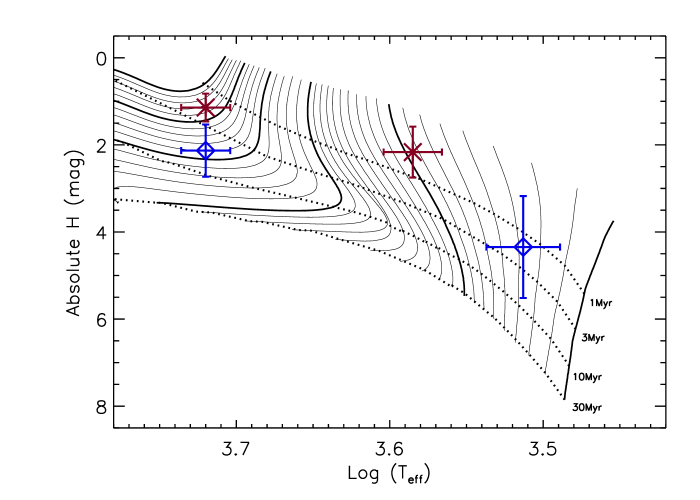
Figure 7: Absolute H magnitude and Log($T_{\rm eff}$) for components of VSB 111 (red asterisks) and VSB 126 (blue diamonds) plotted on the PMS evolutionary tracks from the Dartmouth Stellar Evolution Database for solar metallicity = 0.0, ($\alpha$/Fe) = 0.0, and mixing length = 1.938. The absolute $H$ magnitudes, adopting a distance of 800 pc (Walker 1956), for the components were derived from 2MASS magnitudes and the spectroscopic flux ratios. The isochrones are labeled. The mass tracks start at 0.10M_⊙ and go to 1.0M_⊙ at 0.05M_⊙ intervals then the interval is 0.10M_⊙ from 1.0M_⊙ to 2.5M_⊙. The bold mass tracks represent 0.1M_⊙, 0.5M_⊙, 1.0M_⊙, 1.5M_⊙, 2.0M_⊙, and 2.5M_⊙. The errors in absolute magnitude are most sensitive to distance.

To place the components of the systems on the H-R diagram and estimate the ages and masses of the stars, we tested four sets of PMS evolutionary tracks, by Baraffe et al. (1998), Siess et al. (2000), Dotter et al. (2008), and Tognelli et al. (2011). We used the values of $T_{\rm eff}$ determined from the IR data, described above and given in Table 9, because the IR analysis successfully detected both SB components. For the Dotter et al. and Baraffe et al. tracks we plotted absolute $H$ magnitude to determine the stars’ locations in the H-R diagram. For the Siess et al. and Tognelli et al. tracks we used log(L/L_⊙). For both components in each system we used the distance of 800 pc to convert from apparent to absolute $H$ magnitude and to calculate luminosities as described in §3.4 (Table 9). Tables 11 and 12 list the results for $M_{1}$ and $M_{2}$ as well as the corresponding mass ratios and approximate ages for VSB 111 and VSB 126, respectively. The Dotter et al. tracks are plotted in Figure 7.

The model results for mass are consistent with each other, which is not surprising given the large uncertainties involved in placing the target components on the H-R diagram. The visible light data yield independent values for $T_{\rm eff}$ for the primary stars in both systems (§3.1) so it is possible to test our results using these numbers as well as the IR data. For VSB 111, there is good agreement between the visible light and IR analysis for the primary star; substituting the value of $T_{\rm eff}$ from visible light spectroscopy does not change the H-R diagram results. For VSB 126 the visible light $T_{\rm eff}$ is 5460 K, over 200 K warmer than the IR value of 5248 K (Table 9); however, the only resulting change from using this warmer $T_{\rm eff}$ in the H-R diagram analysis is to increase the age of the primary slightly. The VSB 126 primary star mass estimate remains unchanged as the tracks in this region of the H-R diagram are relatively horizontal. A discrepancy of $>$2 $\sigma$ in the mass ratio is seen between all the evolutionary models and the mass ratio measured from the orbital solutions for VSB 111; the models yield significantly lower mass ratios than the orbital solution. The models also yield different ages for the individual components in both binaries. The age determinations for the secondary stars are consistently younger than the primary components, a systematic bias that follows the trend identified in large population studies (e.g., Hillenbrand 1997). Furthermore, the absolute age for the VSB 111 secondary, $<$1 Myr for all models tested (Table 11), is unrealistically low. However, given the very large uncertainties in the component ages, these results are not significant; for the Dotter et al. (2008) tracks we find age uncertainties of at least $\pm$1 Myr but typically of several Myr (Figure 7).

Torres et al. (2013) studied the four stars in the LkCa 3 system, a young hierarchical quadruple consisting of two short-period spectroscopic binaries. They found a lack of consistency between the dynamically determined orbital and physical characteristics and the properties determined by comparing the location of these stars in the H-R diagram with the models of Baraffe et al. (1998). However, comparison of the Torres et al. observations with the tracks of Dotter et al. (2008) showed good agreement, including between the measured and track-derived mass ratios. The $>$2 $\sigma$ inconsistency described above between the VSB 111 dynamically determined mass ratio and that determined from comparison with the Dotter et al. tracks (Table 11) is thus puzzling. The spectral type, however, may provide a clue. The primary star in VSB 111, K0, is significantly warmer than those of the LkCa 3 primaries, which are between K7 and M2 (Torres et al.). The Dotter et al. tracks may thus provide consistent results between stars of lower masses but the higher mass primaries in the VSB systems possibly span a range of mass tracks for which the results are less homogeneous. This underscores the necessity of testing tracks on a relatively broad sample of systems with a range of masses and mass ratios.

Far more stringent tests of evolutionary tracks would be possible with improvements in the determination of $T_{\rm eff}$ and distance for the stellar components in VSB 111 and VSB 126. Currently, our procedure is to use spectral type standards for the cross-correlation and to identify the young SB components’ spectral types from maximizing the correlation coefficient. $T_{\rm eff}$ is then determined from compilations of spectral type $-$ $T_{\rm eff}$ equivalence, such as those presented in Luhman (1999) and White et al. (1999). To avoid this complication, Torres et al. (2013) adopted the $T_{\rm eff}$ values directly from those assigned by Rojas-Ayala et al. (2012) to several of the template stars used, or from the color/temperature calibrations of Boyajian et al. (2012). In addition to the lack of $T_{\rm eff}$ values for all of our templates from Rojas-Ayala et al. and the lack of colors for the secondary stars in our sample, it is not possible to determine $T_{\rm eff}$ for the primary stars in our sample in this way because they are too hot. Thus we have followed our standard procedure. With a modest investment of observing time in the future, it would be possible to obtain low-resolution ($\sim$2000) K-band spectroscopy and to follow the methodology of Rojas-Ayala et al. and assign $T_{\rm eff}$ values directly to all low-mass ($T_{\rm eff}<4000$) stars in our library of template spectra. An alternative approach must be developed for earlier spectral type stars.

The determination of much improved distance estimates to the target SBs in NGC 2264 is also possible. Combining the angular and physical scales of a system identified as both a visual binary and an SB2 yields an independent distance measurement. For the 902 day period binary VSB 111, VLBA interferometry permits spatial mapping of the binary orbit and will be possible if at least one of the components is a sufficiently strong radio source ($\gtrsim$0.5 mJy), likely given that VSB 111 has a large x-ray flux (Dahm et al. 2007). Based on the orbital period and the total binary mass determined from the Dartmouth tracks, Figure 7, and assuming a distance of 800 pc, the average stellar separation is $\sim$3 mas, easily resolvable by the 0.8 mas FWHM VLBA beam at 8 GHz (4 cm). For VSB 126, GAIA is sufficiently sensitive (standard errors of 15$-$20 $\mu$as for the $V=13.4$ mag of VSB 126; de Bruijne 2012) to resolve the orbit: based on the total mass estimated from the Dartmouth tracks, the period, and d$=$800 pc, the average stellar separation of VSB 126 is 165 $\mu$as. GAIA is scheduled for an October, 2013, launch.

4.2 Rotational Velocities

Based on the IR analysis, VSB 111 has a primary rotational velocity of 30 km s^-1 with a secondary rotational velocity of 15 km s^-1 and VSB 126 has a primary rotational velocity of 15 km s^-1 and a secondary rotational velocity of 8 km s^-1 (Table 9). These are consistent to within 1$\sigma$ of the primary star $v\sin i$ values found in the visible light analysis (section 3.1). We searched the literature for other $v\sin i$ measurements in PMS SB2s (e.g., Ruíz-Rodríguez et al. 2013; Landin et al. 2009; Reipurth et al. 2002; Covino et al. 2001) and found $\sim$35 systems for which the $v\sin i$ values of both SB2 components have been measured. Half of these systems are isolated and half are in young clusters. We examined the ratio $v_{1}\sin i$ to $v_{2}\sin i$ as a function of mass ratio, orbital period, and eccentricity and found that eight systems have a primary star $v\sin i$ value about twice as great as the secondary $v\sin i$ value, including VSB 111 and 126 (Table 13). For the remainder of the systems examined the ratio was close to unity. There were no obvious correlations found when comparing this ratio to $e$, $q$, and orbital period. This result might suggest that rotational evolution between a $v\sin i$ ratio of $\approx$ 2 and a ratio of $\approx$ 1 takes place rapidly, or it may simply be the outcome of observational bias and/or imprecise assignation of $v\sin i$ values. A comparable sample of $v\sin i$ values for main sequence SB2s, from Goldberg et al. (2002), showed no preferential distribution in the primary to secondary star $v\sin i$ ratio. Given the large uncertainties associated with most of the young star $v\sin i$ values from the literature, as well as with our IR results for VSB 111 and VSB 126, i.e. $\pm$5 km s^-1, the odd distribution of $v\sin i$ ratios in young SBs is unlikely to be significant.

4.3 Additional Orbital Properties

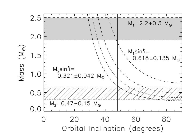
Figure 8: The component masses of VSB 111 as a function of orbital inclination. The values of $M_{1}\sin^{3}i$ and $M_{2}\sin^{3}i$ are given from the orbital solution represented by the curved dashed and dash-dotted lines, respectively. The shaded area represents the primary mass $\pm$1$\sigma$ and the hashed area represents the secondary mass $\pm$1$\sigma$, both derived from the Dotter et al. (2008) tracks. The vertical line shows approximate agreement between all parameters for an orbital inclination of $\sim$48$\,{}^{\circ}$.

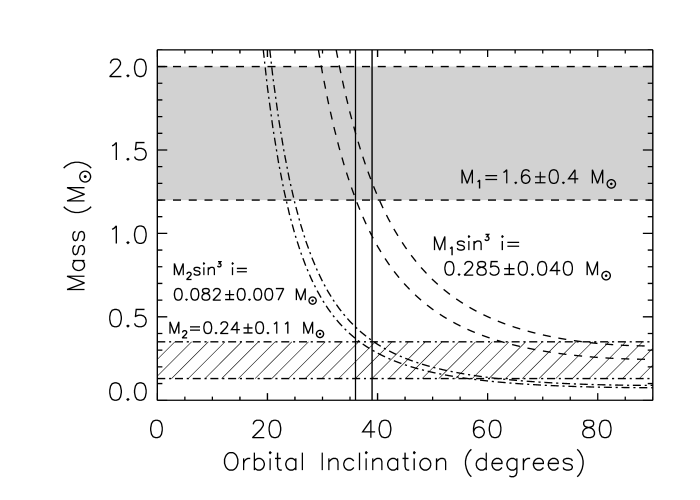
Figure 9: Same as Figure 8 for VSB 126. The vertical lines show agreement between all parameters for an orbital inclination of $\sim 36-39\,^{\circ}$.

We used the model tracks shown in Figure 7 and estimated the mass and associated uncertainties for each star in each binary (Tables 11 and 12). Given the values for $M_{1}\sin^{3}i$ and $M_{2}\sin^{3}i$ determined in the orbital fit for each SB2 (Table 10), we combined these to estimate $i_{orb}$ as illustrated in Figures 8 and 9 for VSB 111 and 126, respectively (Prato et al. 2001; Mace et al. 2012). From these plots we find that for VSB 111 $i_{orb}=48\,^{\circ}$ and for VSB 126 $i_{orb}$ is between $36\,^{\circ}$ and $39\,^{\circ}$.

In §3.4 we estimated the inclinations of the VSB 111 and VSB 126 primary star rotation axes to be 45$\pm 5\,^{\circ}$ and $47^{+9}_{-8}\,{}^{\circ}$, respectively, on the basis of the visible-light data analysis. Unfortunately, without additional information about the visual orbits of these systems, i.e. knowledge of the nodal angles, it is not possible to determine whether there is agreement between the stellar equatorial planes and the orbital planes. However, with facilities such as the VLBA and the GAIA mission, due for launch late in 2013, it will be possible to map out these orbits and to determine the relative orientation of the orbital plane with respect to the stellar equatorial plane. These relative orientations are important for understanding the dynamics of star-orbit interactions, which may in turn shape the planet formation and evolution environment. By directly and accurately measuring the orbital inclination, it will also be possible to derive the model-independent absolute component masses directly.

4.4 NGC 2264

The locations of VSB 111 and 126 are separated by $\sim$0.02 pc in right ascension and $\sim$1.9 pc in declination, assuming an 800 pc distance to NGC 2264. VSB 111, with $\gamma$ = 25.31 km s^-1 (Table 10), lies very close to the core of a ¹³CO cloud, as determined from visual inspection of Figure 1 from Fűrész et al. (2006). VSB 126, with $\gamma$ = 17.16 km s^-1 (Table 10), does not appear to be associated with any cloud cores. If VSB 111 is actually associated with this cloud core, this location is consistent with the age of VSB 111 being younger than that of VSB 126, as suggested by Figure 7.

Both $\gamma$ velocities for VSB 111 and VSB 126 fall within the cluster distribution range for membership: Fűrész et al. (2006) found that NGC 2264 is hierarchically structured with a north-south RV gradient, which increases with increasing declination. Stars in the northern half of the cluster have an overall higher RV than the stars in the southern half. The mean RV for stars with declination near +9$\,{}^{\circ}$ $50\arcmin$  is $\sim$27 km s^-1 and the mean RV for stars with declination near +9$\,{}^{\circ}$ $37\arcmin$  is $\sim$16 km s^-1. Stars that are in the same region of NGC 2264 as VSB 111 and VSB 126 thus have RVs that are consistent with these binaries’ $\gamma$ velocities.

Interstellar reddening toward NGC 2264 is fortuitously negligible. This not only ensures that the targets are as bright as possible given their relatively large distances but also facilitates the measurement of luminosity, which may be hindered by the accurate determination of A_V. The largest value of reddening was determined by Rebull et al. (2002) to be E(B-V)=0.15$\pm$0.03 for a distance of 760 pc. The lowest value of reddening was determined by Feldbrugge & van Genderen (1991) to be E(B-V)=0.04 at a distance of 700 pc. There is a dark cloud of dense dust that lies directly behind NGC 2264, reducing the possibility of background stars contaminating the field. The low value for extinction found in the literature agree with the values we calculated of A${}_{V}=0$ for both systems (§3.4).

5 Summary

High-resolution, IR spectra were obtained for the young SBs VSB 111 and VSB 126 in NGC 2264 and combined with visible light spectra. One- and two-dimensional cross-correlation was used to obtain the RVs and orbital parameters for these systems. VSB 111 has a period of $\sim$902 days, an eccentricity of 0.79$\pm$0.01, and a mass ratio of 0.52$\pm$0.05 while VSB 126 has a period of $\sim$12.9 days, an eccentricity of 0.18$\pm$0.02, and a mass ratio of 0.29$\pm$0.02. The eccentricity of VSB 111 is the second highest known for a PMS SB2 measured to date (Mace et al. 2009). We determined the stellar rotation periods for the primary components of both systems, $\sim$4 and $\sim$6 days for VSB 111 and VSB 126, respectively.

Our analysis indirectly provided additional physical properties for both stars in each SB2, such as $T_{\rm eff}$, binary flux ratio, luminosity, and $v\sin i$. These results in turn allowed us to place both stars in each binary on an H-R diagram for comparison with model calculations of PMS evolution, effectively testing the evolutionary tracks against our dynamical results. By using the model-determined masses, we estimated the binaries’ orbital inclinations; we also found the inclination angles of the primary stars’ equatorial planes. With observations of the angularly resolved orbits of these NGC 2264 members, through VLBI and GAIA, the dynamical determination of the orbital inclination and orientation (i.e., the nodal angle) will be possible. These measurements in turn yield the absolute component masses, distance to the system, and the relative inclinations of the primary stars with respect to the orbital planes.

Determining the spectroscopic orbital solutions for these two young SB2s inches us closer to our immediate goal to significantly increase the number of such systems in order to better understand and improve models of binary star formation, and to help anchor theoretical evolutionary tracks with solid dynamical data.

We are grateful to G. Mace, M. Simon, K. Covey, and J. Patience for useful discussions and comments throughout the progress of this project. We thank Joel Aycock, Gary Puniwai, Gabrelle Saurage, and Cynthia Wilburn for their superb telescope support and Randy Campbell, Al Conrad, Jim Lyke, Barbara Schaefer, and Greg Wirth for their dedicated technical and logistical support. We are grateful to P. Berlind, J. Caruso, R. J. Davis, L. Hartmann, E. Horine, A. Milone, J. Peters, J. Stauffer, R. P. Stefanik, and S. Tokarz for help in obtaining the visible-light spectra of VSB 111 and VSB 126. This work was supported in part by the NSF grant AST-1009136 to L.P.; G.T. acknowledges partial support from NSF grant AST-1007992. Data presented herein were obtained at the W. M. Keck Observatory from telescope time allocated to the National Aeronautics and Space Administration through the agency s scientific partnership with the California Institute of Technology and the University of California. Keck telescope time was also granted by NOAO, through the Telescope System Instrumentation Program (TSIP). TSIP is funded by NSF. The Observatory was made possible by the generous financial support of the W. M. Keck Foundation. This work made use of the SIMBAD database, the Vizier database, the NASA Astrophysics Data System, and the data products from the Two Micron All Sky Survey, which is a joint project of the University of Massachusetts and the Infrared Processing and Analysis Center/California Institute of Technology, funded by the National Aeronautics and Space Administration and the NSF. This publication also made use of data products from the Wide-field Infrared Survey Explorer, which is a joint project of the University of California, Los Angeles, and the Jet Propulsion Laboratory/California Institute of Technology, funded by the National Aeronautics and Space Administration. We recognize and acknowledge the significant cultural role that the summit of Mauna Kea plays within the indigenous Hawaiian community and are grateful for the opportunity to conduct observations from this special mountain.

Table 1: Target Properties

Property	VSB 111	VSB 126
R.A. (J2000)	06 41 04.41	06 41 07.778
Dec. (J2000)	+09 51 50.1	+09 44 03.00
$U$ (mag)	13.677$\pm$0.004	14.391$\pm$0.031
$B$ (mag)	13.60	14.17
$V$ (mag)	12.68	13.39
$J$ (mag)	10.737$\pm$0.023	11.887$\pm$0.022
$H$ (mag)	10.300$\pm$0.024	11.513$\pm$0.026
$K$ (mag)	10.145$\pm$0.027	11.383$\pm$0.025
H$\alpha$ EW (Å)	-0.3	-1.9

Table 2: VSB 111 Visible-Light Radial Velocities

HJD	$v$1$\pm$$\sigma$ (km s-1)	Phase
2445714.8925	21.3$\pm$0.9	0.1975
2445747.6330	19.9$\pm$1.8	0.2338
2446066.9770	26.0$\pm$1.4	0.5878
2446076.8868	26.1$\pm$1.0	0.5988
2446420.9011	32.9$\pm$1.7	0.9802
2446489.7238	14.5$\pm$1.2	0.0565
2446776.7760	25.4$\pm$1.5	0.3747
2446802.9369	26.5$\pm$1.2	0.4037
2446814.9734	23.1$\pm$1.2	0.4170
2446873.6357	25.7$\pm$1.2	0.4821
2446873.6538	25.5$\pm$2.4	0.4821
2447074.0159	30.1$\pm$1.5	0.7042
2447076.9919	29.5$\pm$0.8	0.7075
2447079.9911	29.9$\pm$1.6	0.7108
2447127.9563	32.2$\pm$1.3	0.7640
2447128.8350	29.9$\pm$1.6	0.7650
2447138.8504	29.9$\pm$1.0	0.7761
2447157.9513	29.7$\pm$1.2	0.7972
2447169.9786	31.1$\pm$1.2	0.8106
2447192.6830	31.4$\pm$1.6	0.8357
2447220.7105	31.4$\pm$1.3	0.8668
2447250.7112	30.2$\pm$1.4	0.9001
2447428.9314	15.5$\pm$1.1	0.0976
2447489.8353	20.6$\pm$1.4	0.1651
2447493.8657	20.8$\pm$1.0	0.1696
2447523.9220	24.5$\pm$1.1	0.2029
2447549.9107	23.8$\pm$0.8	0.2317
2447573.7981	22.0$\pm$1.4	0.2582
2447580.7045	23.5$\pm$1.0	0.2659
2447641.6147	23.0$\pm$1.8	0.3334
2447642.6205	22.8$\pm$1.5	0.3345
2447791.9773	25.8$\pm$1.1	0.5001
2447811.9797	26.3$\pm$1.6	0.5223
2447812.9739	25.2$\pm$1.1	0.5234
2447845.9494	28.6$\pm$1.0	0.5599
2447898.8962	26.9$\pm$1.1	0.6186
2447906.7812	27.8$\pm$1.4	0.6274
2447958.7219	28.9$\pm$1.1	0.6849
2448168.9877	33.5$\pm$1.1	0.9180
2448200.9677	33.6$\pm$1.5	0.9535
2448256.7928	9.3$\pm$1.2	0.0154
2448261.6991	10.0$\pm$1.9	0.0208
2448281.7687	13.8$\pm$1.5	0.0208
2448284.7245	10.9$\pm$1.4	0.0463
2448288.7069	13.9$\pm$0.8	0.0507
2448340.6732	18.5$\pm$1.4	0.1084
2448346.6417	18.2$\pm$0.9	0.1150
2448347.6792	20.0$\pm$1.4	0.1161
2448367.6272	18.7$\pm$2.3	0.1382
2448370.6468	17.3$\pm$2.1	0.1416
2448669.7119	26.6$\pm$1.0	0.4731
2448671.8058	26.4$\pm$1.2	0.4754
2448910.9782	30.8$\pm$1.0	0.7406
2449647.9617	26.8$\pm$1.1	0.5576
2449701.9633	25.2$\pm$1.3	0.8174
2450001.9827	32.7$\pm$0.8	0.9500
2450026.8712	31.7$\pm$1.9	0.9776
2450029.9581	29.2$\pm$0.9	0.9810
2450034.9645	27.5$\pm$1.0	0.9866
2450037.0311	25.4$\pm$1.3	0.9889
2450038.8478	24.8$\pm$1.6	0.9909
2450051.9235	11.3$\pm$1.0	0.0054
2450059.8782	10.3$\pm$1.0	0.0142
2450064.8144	9.0$\pm$1.5	0.0197
2450080.7933	10.5$\pm$3.0	0.0374
2450081.8739	13.2$\pm$1.6	0.0386
2450084.8209	10.5$\pm$0.9	0.0418
2450091.8166	13.5$\pm$1.3	0.0496

Table 3: VSB 126 Visible-Light Radial Velocities

HJD	$v$1$\pm$$\sigma$ (km s-1)	Phase
2445783.6412	9.0$\pm$1.0	0.1224
2446077.7737	5.2$\pm$0.9	0.8804
2446775.9909	3.1$\pm$0.7	0.9038
2447075.9919	7.2$\pm$0.9	0.1159
2447078.9952	25.9$\pm$1.1	0.3483
2447127.9675	11.5$\pm$1.0	0.1374
2447128.8485	19.2$\pm$1.0	0.2056
2447138.8614	0.7$\pm$1.0	0.9803
2447157.9395	30.1$\pm$0.6	0.4564
2447158.9747	27.9$\pm$0.8	0.5365
2447159.9427	26.8$\pm$0.8	0.6114
2447169.9634	28.5$\pm$1.3	0.3868
2447199.7030	22.8$\pm$1.3	0.6878
2447200.7497	14.6$\pm$1.1	0.7688
2447220.6977	26.8$\pm$0.8	0.3122
2447222.7006	28.5$\pm$1.5	0.4672
2447224.6626	22.6$\pm$2.1	0.6190
2447229.6414	-0.1$\pm$1.0	0.0043
2447230.6267	5.0$\pm$0.9	0.0805
2447250.7040	24.5$\pm$0.7	0.6339
2447427.9928	26.4$\pm$0.9	0.3514
2447428.9520	29.2$\pm$1.0	0.4256
2447429.9625	28.9$\pm$0.9	0.5038
2447489.8436	12.6$\pm$0.8	0.1370
2447493.8731	29.0$\pm$0.8	0.4487
2447524.9283	6.5$\pm$0.9	0.8516
2447549.9192	14.4$\pm$0.6	0.7852
2447845.9554	21.8$\pm$0.9	0.6905
2448669.7216	30.3$\pm$1.3	0.4280

Table 4: VSB 111 IR Radial Velocities

UT Date of Observations	HJD	$v$1$\pm$$\sigma$ (km s-1)	$v$2$\pm$$\sigma$ (km s-1)	Phase
2001 Dec 31	2452274.94279	25.6$\pm$1.0	24.4$\pm$2.0	0.4697
2002 Feb 6	2452311.86271	27.1$\pm$1.0	23.5$\pm$2.0	0.5106
2002 Dec 14	2452623.04253	32.7$\pm$1.0	14.4$\pm$2.0	0.8556
2004 Jan 28	2453032.84263	23.6$\pm$1.0	28.5$\pm$2.0	0.3099
2004 Dec 26	2453366.04274	27.7$\pm$1.0	20.5$\pm$2.0	0.6793
2010 Dec 10	2455543.11876	15.7$\pm$1.0	43.3$\pm$2.0	0.0927
2012 Jan 11	2455937.93446	26.3$\pm$1.0	23.4$\pm$2.0	0.5304

Table 5: VSB 126 IR Radial Velocities

UT Date of Observations	HJD	$v$1$\pm$$\sigma$ (km s-1)	$v$2$\pm$$\sigma$ (km s-1)	Phase
2002 Jan 1	2452275.91504	29.1$\pm$1.0	-25.3$\pm$5.0	0.4511
2002 Feb 5	2452310.90655	13.5$\pm$1.0	18.4$\pm$5.0	0.1585
2002 Dec 14	2452623.07869	24.4$\pm$1.0	-15.7$\pm$5.0	0.3123
2002 Dec 22	2452631.03900	1.3$\pm$1.0	71.7$\pm$5.0	0.9282
2004 Jan 27	2453031.95005	1.3$\pm$1.0	76.5$\pm$5.0	0.9481
2004 Dec 25	2453365.06614	20.9$\pm$1.0	11.3$\pm$5.0	0.7224

Table 6: Photometric Comparison Stars

ID	Walker	RA (J2000)	Dec (J2000)	$V$(mag)	$B$ - $V$	aliases
1	NGC 2264 086	6 40 37.49	+09 54 57.8	11.73	0.63	NSV 17013
2	NGC 2264 216	6 41 31.50	+09 54 54.8	11.90	0.77	NSV 3156
3	NGC 2264 190	6 41 31.81	+09 55 43.9	12.34	0.62	NSV 17104
4	NGC 2264 125	6 40 56.97	+09 48 40.7	12.32	0.60	NSV 17059
5	NGC 2264 151	6 41 02.96	+09 47 54.3	12.57	0.49	NSV 3117

Table 7: VSB 111 Photometry

BJD	$V$ mag $\pm$$\sigma$	Phase
2456204.87406	12.577$\pm$0.005	0.033
2456204.89336	12.581$\pm$0.005	0.038
2456204.93308	12.590$\pm$0.004	0.049
2456204.95158	12.587$\pm$0.004	0.054
2456204.96819	12.590$\pm$0.004	0.058
2456204.98598	12.590$\pm$0.004	0.631
2456205.01121	12.590$\pm$0.004	0.070
2456205.01694	12.588$\pm$0.004	0.071
2456205.87830	12.642$\pm$0.004	0.302
2456205.93331	12.645$\pm$0.004	0.316
2456205.94994	12.644$\pm$0.004	0.321
2456205.97125	12.646$\pm$0.004	0.327
2456205.98655	12.646$\pm$0.004	0.331
2456206.01396	12.650$\pm$0.004	0.338
2456206.01763	12.648$\pm$0.004	0.339
2456207.85301	12.619$\pm$0.005	0.830
2456207.92283	12.617$\pm$0.005	0.848
2456207.95936	12.613$\pm$0.005	0.858
2456208.01980	12.607$\pm$0.004	0.874
2456208.88059	12.604$\pm$0.004	0.104
2456208.94489	12.610$\pm$0.004	0.122
2456208.97615	12.610$\pm$0.004	0.130
2456209.87799	12.640$\pm$0.004	0.371
2456209.94233	12.639$\pm$0.004	0.388
2456209.97354	12.636$\pm$0.007	0.397
2456210.87131	12.642$\pm$0.004	0.637
2456210.93555	12.639$\pm$0.004	0.654
2456210.96680	12.644$\pm$0.004	0.662
2456211.01759	12.643$\pm$0.004	0.676
2456211.87116	12.601$\pm$0.004	0.904
2456211.93582	12.602$\pm$0.004	0.921
2456211.96794	12.602$\pm$0.004	0.930
2456212.01888	12.600$\pm$0.003	0.944

Table 8: VSB 126 Photometry

BJD	$V$ mag $\pm$$\sigma$	Phase
2456204.87406	13.505$\pm$0.008	0.022
2456204.89336	13.506$\pm$0.008	0.025
2456204.93308	13.504$\pm$0.006	0.032
2456204.95158	13.503$\pm$0.006	0.035
2456204.96819	13.508$\pm$0.006	0.041
2456204.98598	13.502$\pm$0.005	0.046
2456205.01121	13.503$\pm$0.005	0.047
2456205.01694	13.504$\pm$0.006	0.198
2456205.87830	13.524$\pm$0.006	0.207
2456205.93331	13.520$\pm$0.006	0.210
2456205.94994	13.523$\pm$0.006	0.214
2456205.97125	13.515$\pm$0.005	0.217
2456205.98655	13.521$\pm$0.005	0.221
2456206.01396	13.520$\pm$0.005	0.222
2456206.01763	13.518$\pm$0.006	0.543
2456207.85301	13.536$\pm$0.009	0.556
2456207.92283	13.540$\pm$0.008	0.572
2456207.95936	13.542$\pm$0.008	0.723
2456208.01980	13.541$\pm$0.006	0.735
2456208.88059	13.527$\pm$0.006	0.740
2456208.94489	13.527$\pm$0.005	0.898
2456208.97615	13.518$\pm$0.005	0.909
2456209.87799	13.511$\pm$0.005	0.915
2456209.94233	13.506$\pm$0.006	0.072
2456209.97354	13.519$\pm$0.011	0.083
2456210.87131	13.503$\pm$0.005	0.098
2456210.93555	13.499$\pm$0.005	0.247
2456210.96680	13.505$\pm$0.005	0.258
2456211.01759	13.502$\pm$0.005	0.264
2456211.87116	13.520$\pm$0.005	0.273

Table 9: Physical Properties of VSB 111 and VSB 126

	IR	IR	Visible	Visible
Property	VSB 111	VSB 126	VSB 111	VSB 126
Primary Rotation Period (days)	$-$	$-$	3.74$\pm$0.02	5.71$\pm$0.07
Primary Spectral Type	K0$\pm$1	K0$\pm$1	$-$	$-$
Secondary Spectral Type	M0$\pm$1	M4$\pm$1	$-$	$-$
Primary $T_{\rm eff}$ (K)	5248$\pm$194	5248$\pm$194	5300$\pm$100	5460$\pm$100
Secondary $T_{\rm eff}$ (K)	3846$\pm$192	3258$\pm$180	$-$	$-$
Primary $v\sin i$ (km s-1)	30$\pm$5	15$\pm$5	31$\pm$2	13$\pm$2
Secondary $v\sin i$ (km s-1)	15$\pm$5	8$\pm$5	$-$	$-$
log(L1/L⊙)	$0.87^{+0.16}_{-0.17}$	0.47$\pm 0.17$	0.87$\pm$0.07	$0.51^{+0.07}_{-0.08}$
log(L2/L⊙)	$0.22^{+0.28}_{-0.19}$	$-0.72^{+0.26}_{-0.34}$	$-$	$-$
R1 (R⊙)	$3.29^{+0.88}_{-0.73}$	$2.09^{+0.57}_{-0.47}$	$3.25^{+0.29}_{-0.28}$	$2.00^{+0.19}_{-0.17}$

Table 10: Orbital Elements and Properties for VSB 111 and VSB 126

Element/Property	VSB 111	VSB 126
P (days)	902.1$\pm$0.9	12.9244$\pm$0.0002
$\gamma$ (km s-1)	25.31$\pm$0.16	17.16$\pm$0.17
K1 (km s-1)	12.00$\pm$0.32	14.74$\pm$0.24
K2 (km s-1)	23.1$\pm$2.2	51.3$\pm$2.8
$e$	0.788$\pm$0.008	0.18$\pm$0.02
$\omega$ (deg)	115.6$\pm$2.2	190.1$\pm$5.3
T +2,444,000(HJD)	634.6$\pm$5.3	605.94$\pm$0.17
$M_{1}\sin^{3}i$ (M⊙)	0.618$\pm$0.135	0.285$\pm$0.040
$M_{2}\sin^{3}i$ (M⊙)	0.321$\pm$0.042	0.082$\pm$0.007
q$=$$M_{2}$/$M_{1}$	0.52$\pm$0.05	0.29$\pm$0.02
a1sin $i$ (Gm)	91.6$\pm$2.0	2.58$\pm$0.04
a2sin $i$ (Gm)	176.1$\pm$16.3	8.96$\pm$0.49

Table 11: Evolutionary Track Comparisons for VSB 111 ($q_{obs}$ = 0.52$\pm$0.05)

Tracks	M1 (M⊙)	Age (Myr)	M2 (M⊙)	Age (Myr)	$q\pm 1\sigma$
Baraffe et al. (1998)	-	-	0.63$\pm$0.10	$<$ 1	-
Tognelli et al. (2011)	2.3$\pm$0.3	2$\pm$1	0.45$\pm$0.20	0.5$\pm$1.0	0.2$\pm$0.1
Siess et al. (2000)	2.1$\pm$0.3	3$\pm$2	0.41$\pm$0.10	0.3$\pm$0.5	0.2$\pm$0.1
Dotter et al. (2008)	2.2$\pm$0.3	2$\pm$1	0.47$\pm$0.15	$<$1	0.2$\pm$0.1

Table 12: Evolutionary Track Comparisons for VSB 126 ($q_{obs}$ = 0.29$\pm$0.02)

Tracks	M1 (M⊙)	Age (Myr)	M2 (M⊙)	Age (Myr)	$q\pm 1\sigma$
Baraffe et al. (1998)	-	-	0.28$\pm$0.14	2$\pm$5	-
Tognelli et al. (2011)	1.7$\pm$0.3	4$\pm$2	0.25$\pm$0.12	2$\pm$3	0.2$\pm$0.1
Siess et al. (2000)	1.6$\pm$0.3	5$\pm$3	0.17$\pm$0.07	1$\pm$2	0.1$\pm$0.1
Dotter et al. (2008)	1.6$\pm$0.4	5$\pm$4	0.24$\pm$0.11	2$\pm$6	0.2$\pm$0.1

Table 13: Properties of PMS SB2s with $v_{1}\sin i$ twice as large as $v_{2}\sin i$

System	$v{{}_{1}}\sin i$ (km s-1)	$v{{}_{2}}\sin i$ (km s-1)	$e$	$q$	Period (days)
VSB 111	30$\pm$5	15$\pm$5	0.79	0.52	902.1
VSB 126	15$\pm$5	8$\pm$5	0.18	0.29	12.92
RX J0539.9$+$0956	80$\pm$10	40$\pm$5	0.27	0.7	1118.3
RX J0513.1$+$0851	60$\pm$10	30$\pm$5	0.067	0.44	4.018
EK Cep	23$\pm$2	10.5$\pm$2.0	0.109	0.55	4.43
Parenago 2494	22.0$\pm$2.5	11.4$\pm$2.0	0.257	0.71	19.48
RX J0441.0-0839	2$\pm$1	1$\pm$1	0.216	0.82	13.56
RX J0350.5-1355	19$\pm$2	7$\pm$1	0.0	0.92	9.28

Figure 1: Seven reduced spectra for VSB 111 with the correction for heliocentric motion taken into account. UT dates are specified with corresponding spectra.

Figure 2: Six reduced spectra for VSB 126 with the correction for heliocentric motion taken into account. UT dates are specified with corresponding spectra.

References

- Baraffe et al. (1998) Baraffe, I., Chabrier, G., Allard, F., & Hauschildt, P. H. 1998, A&A, 337, 403
- Bate (2009) Bate, M. R. 2009, MNRAS, 397, 232
- Boyajian et al. (2012) Boyajian, T. S., von Braun, K., van Belle, G., McAlister, H. A., ten Brummelaar, T. A., Kane, S. R., Muirhead, P. S., Jones, J., White, R., Schaefer, G., Ciardi, D., Henry, T., López-Morales, M., Ridgway, S., Gies, D., Jao, W. C, Rojas-Ayala, B., Parks, J. R., Sturmann, L., Sturmann, J., Turner, N. H., Farrington, C., Goldfinger, P. J., & Berger, D. H. 2012, ApJ, 757, 112
- Buie (2010) Buie, M. W. 2010, Advances in Astronomy, 2010, 130172
- Charbonneau (1995) Charbonneau, P. 1995, ApJS, 101, 309
- Covino et al. (2001) Covino, E., Melo, C., Alcalá, J. M., Torres, G., Fernández, M., Frasca, A., & Paladino, R. 2001, A&A, 375, 130
- Dahm et al. (2007) Dahm, S. E., Simon, T., Proszkow, E. M., & Patten, B. M., 2007, AJ, 134, 999
- Dahm (2008) Dahm, S. E., 2008, Handbook of Star Forming Regions, Volume I, 966
- de Bruijne (2012) de Bruijne, J. H. J. 2012, Ap&SS, 341, 31
- Dotter et al. (2008) Dotter, A., Chaboyer, B., Jevremović, D., Kostov, V., Baron, E., & Ferguson, J. W. 2008, ApJS, 178, 89
- Feldbrugge & van Genderen (1991) Feldbrugge, P. T. M. & van Genderen, A. M., 1991, A&A, 91, 209
- Flaccomio et al. (1999) Flaccomio, E., Micela, G., Sciortino, S., Favata, F., Corbally, C., & Tomaney, A., 1999, A&A, 345, 521
- Flaccomio et al. (2006) Flaccomio, E., Micela, G., & Sciortino, S., 2006, A&A, 455, 903
- Fűrész et al. (2006) Fűrész, G., Hartmann, L. W., Szentgyorgyi, A. H., Ridge, N. A., Rebull, L., Stauffer, J., Latham, D. W., Conroy, M. A., Fabricant, D. G., & Roll, J. 2006, AJ, 648, 1090
- Goldberg et al. (2002) Goldberg, D., Mazeh, T., Latham, D. W., Stefanik, R. P., Carney, B. W., & Laird, J. B. 2002, AJ, 124, 1132
- Haisch et al. (2001) Haisch, K. E., Lada, E. A., & Lada, C. L. 2001, ApJ, 553, L153
- Hillenbrand (1997) Hillenbrand, L. A. 1997, AJ, 113, 1733
- Hillenbrand & White (2004) Hillenbrand, L. A., & White, R. J. 2004, ApJ, 604, 741
- Kearns & Herbst (1998) Kearns, K. E., & Herbst, W. 1998, AJ, 116, 261
- Landin et al. (2009) Landin, N. R., Mendes, L. T. S., & Vaz, L. P. R. 2009, A&A, 494, 209L
- Latham (1992) Latham, D. W. 1992, in Astronomical Society of the Pacific Conference Series, Vol. 32, IAU Colloq. 135: Complementary Approaches to Double and Multiple Star Research, ed. H. A. McAlister & W. I. Hartkopf, 596
- Latham et al. (2002) Latham, D. W., Stefanik, R. P., Torres, G., Davis, R. J., Mazeh, T., Carney, B. W., Laird, J. B., & Morse, J. A. 2002, AJ, 124, 1144
- Luhman (1999) Luhman, K. L. 1999, ApJ, 525, 466
- Luhman et al. (2003) Luhman, K. L., Briceño, C., Stauffer, J. R., Hartmann, L., Barrado Y Navascués, D., & Caldwell, N. 2003, ApJ, 590, 348
- Mace et al. (2009) Mace, G. N., Prato, L., Wasserman, L. H., Schaefer, G. H., Franz, O. G., & Simon, M. 2009, AJ, 137, 3487
- Mace et al. (2012) Mace, G. N., Prato, L., Torres, G., Wasserman, L. H., Mathieu, R. D., & McLean, I. S. 2012, AJ, 144, 55
- Makidon et al. (2004) Makidon, R. B., Rebull, L. M., Strom, S. E., Adams, M. T., & Patten, B. M. 2004, AJ, 127, 2228
- Mathieu (1994) Mathieu, R. 1994, A&A, 32, 465
- Mazeh et al. (2002) Mazeh, T., Prato, L., Simon, M., Goldberg, E., Norman, D., & Zucker, S. 2002, ApJ, 564, 1007
- Mazeh et al. (2003) Mazeh, T., Simon, M., Prato, L., Markus, B., & Zucker, S. 2003, ApJ, 599, 1344
- McLean et al. (1998) McLean, I. S., Becklin, E. E. & Bendiksen, O. et al. 1998, Proc. SPIE, 3354, 566
- McLean et al. (2000) McLean, I. S., Graham, J. R., & Becklin, E. E. et al. 2000, Proc. SPIE, 4008, 1048
- Mendoza & Gómez (1980) Mendoza, E. E & Gómez, T. 1980, MNRAS, 190, 623
- Nordström et al. (1994) Nordström, B., Latham, D. W., Morse, J. A., 1994, A&A, 287, 338
- Pérez et al. (1987) Pérez, M. R., Thé, P. S., & Westerlund, B. E. 1987, PASP, 99, 1050
- Prato (1998) Prato, L., 1998, Ph.D. thesis, SUNY Stony Brook
- Prato et al. (2001) Prato, L., Ghez, A. M., Piña, R. K., Telesco, C. M., Fisher, R. S., Wizinowich, P., Lai, O., Acton, D. S., & Stomski, P. 2001, ApJ, 549, 590
- Prato et al. (2002) Prato, L., Simon, M., Mazeh, T., McLean, I. S., Norman, D., & Zucker, S. 2002, ApJ, 569, 863
- Prato et al. (2003) Prato, L., Greene, T. P., & Simon, M. 2003, ApJ, 584, 853
- Press et al. (1992) Press, W. H., Teukolsky, S. A., Vetterling, W. T., & Flannery, B. P. 1992, Numerical Recipes in Fortran: The Art of Scientific Computing (2nd ed.; Cambridge: Cambridge Univ. Press)
- Ramirez et al. (2004) Ramirez, S. V., Rebull, L., Stauffer, J., Hearty, T., Hillenbrand, L. A. 2004, AJ, 127, 2659
- Rebull et al. (2002) Rebull, L. M., Makidon, R. B., Strom, S. E., Hillenbrand, L. A., Birmingham, A., Patten, B. M., Jones, B. F., Yagi, H., & Adams, M. T. 2002, AJ, 123, 1528
- Reipurth et al. (2002) Reipurth, B., Lindgren, H., Mayor, M., Mermilliod, J., & Cramer, N. 2002, AJ, 124, 2813
- Rojas-Ayala et al. (2012) Rojas-Ayala, B., Covey, K. R., Muirhead, P. S., & Lloyd, J. P. 2012, ApJ, 748, 93
- Rousselot et al. (2000) Rousselot, P., Lidman, C., Cuby, J.-G., Moreels, G., & Monnet, G. 2000, A&A, 354, 1134
- Ruíz-Rodríguez et al. (2013) Ruíz-Rodríguez, D., Prato, L., Torres, G., Wasserman, L., & Neuhäuser, R. 2013, AJ, 145, 162
- Sagar & Joshi (1983) Sagar, R. & Joshi, U. C. 1983, MNRAS, 205, 747
- Samus et al. (2012) Samus, N. N., Durlevich, O. V., Kazarovets, E. V., Kireeva, N. N., Pastukhova, E. N., & Zharova, A. V. 2012, General Catalog of Variable Stars
- Schaefer et al. (2012) Schaefer, G. H., Prato, L., Simon, M., & Zavala, R. T. 2012, ApJ, 756, 120
- Siess et al. (2000) Siess, L., Dufour, E., & Forestini, M. 2000, A&A, 358, 593
- Simon (2008) Simon, M. 2008, The Power of Optical/IR Interferometry: Recent Scientific Results and 2nd Generation, 227
- Sung et al. (1997) Sung, H., Bessell, M. S., & Lee, S.-W. 1997, AJ, 114, 2644
- Sung et al. (2004) Sung, H., Bessell, M. S., & Chun, M. Y. 2004, AJ, 128, 1684
- Tognelli et al. (2011) Tognelli, E., Prada Moroni, P. G., & Degl’ Innocenti, S. 2011, A&A, 533, A109
- Tokunaga (2000) Tokunaga, A. T. 2000, Allen’s Astrophysical Quantities, ed. 4, A. N. Cox (New York: Springer-Verlag), 143
- Torres et al. (1997) Torres, G., Stefanik, R. P., & Latham, D. W. 1997, AJ, 474, 256
- Torres et al. (2002) Torres, G., Neuhäuser, R., & Guenther, E. W. 2002, AJ, 123, 1701
- Torres et al. (2013) Torres G., Ruíz-Rodríguez, D., Badenas, M., Prato, L., Schaefer, G. H., Wasserman, L. H., Mathieu, R. D., & Latham, D. W. 2013, ApJ, 698, 242
- Vasilevskis et al. (1965) Vasilevskis, S., Sanders, W. L., & Balz, Jr, A. G. A. 1965, AJ, 70, 10, 797
- Walker (1956) Walker, M. F. 1956, ApJ, Supplement Series, 2, 365
- Warner (2007) Warner, B. D. 2007, Minor Planet Bulletin, 34, 113
- Warner (2011) Warner, B. D. 2011, MPO Software, Canopus version, 10.4.0.6
- White et al. (1999) White, R. J., Ghez, A. M., Reid, I. N., & Schultz, G. 1999, ApJ, 520, 811
- Zucker & Mazeh (1994) Zucker, S., & Mazeh, T. 1994, ApJ, 420, 806