Brillouin zone labelling for quasicrystals

Abstract

We propose a scheme to determine the energy-band dispersion of quasicrystals which does not require any periodic approximation and which directly provides the correct structure of the extended Brillouin zones. In the gap labelling viewpoint, this allow to transpose the measure of the integrated density-of-states to the measure of the effective Brillouin-zone areas that are uniquely determined by the position of the Bragg peaks. Moreover we show that the Bragg vectors can be determined by the stability analysis of the law of recurrence used to generate the quasicrystal. Our analysis of the gap labelling in the quasi-momentum space opens the way to an experimental proof of the gap labelling itself within the framework of an optics experiment, polaritons, or with ultracold atoms.

Introduction

Quasicrystals are alloys that show long range order but possess symmetries that prevent them to be crystals. The first examples observed were rapidly quenched alloys of Aluminum and Manganese exhibiting icosahedral symmetry. From their spectacular experimental realization in the early 80’s [1] to their very recent discovery as natural objects in the Kamtchatka mountains [2], quasicrystals have been the subject of very active research, whose domains extend far beyond the scope of solid state physics. Quasicrystals can also be reproduced with dielectric materials [3] or via the interference of laser beams [4] and thus they are studied not only for the transport of electrons, but also of light, matter waves or even quasiparticles such as polaritons [5]. For all these cases the knowledge of the energy-band dispersion is a crucial concept which is much more sophisticated than in the crystal case.

For a periodic crystal, the diffraction spectrum is pure point with a lattice structure and the energy spectrum is organized in bands separated by gaps. All bands can be calculated in the fundamental Brillouin zone (BZ) that is the primitive cell of the reciprocal lattice. This is possible because of the equivalence of the BZs, meaning that the area of each zone is the same and that different BZs are connected by the Bragg vectors. It follows that the number of states in each band is the same and that the integrated density of states (IDOS) ${\mathcal{N}}(E)$ is a staircase with identical steps. For quasicrystals the situation is a bit different. The diffraction spectrum is again pure point but it does not exist a fundamental BZ. On the other hand, the IDOS is again a staircase, despite its more sophisticated structure, and thus one can continue to speak about bands and gaps. The heights of the steps are all different and one can use these heights to label the gaps. One can enumerate the gaps in a way that depends only on the geometry of the quasicrystal and not on the nature of the potential it induces. In particular, for a potential which varies with a parameter, the labelling remains invariant under the parameter evolution (this is the subject of the so-called gap labelling theory [6, 7, 8, 9]). For instance it was shown that for Fibonacci or Penrose tilings, in the limit of an infinite sample of quasicrystal, and when $E$ belongs to a gap, the IDOS reads:

$${\mathcal{N}}(E)={z}_{i_{1}}+\lambda{z}_{i_{2}}$$ (1)

where $\lambda=(\sqrt{5}+1)/2$ is the golden number and the $z_{i}$’s are relative integers. Morover, the staircase is a devil’s staircase: each step is divided in smaller steps and each smaller step is divided in steps even smaller, etc…, and the spectrum is a Cantor set. At a finite but large fixed energy resolution one can identify the main gaps of the staircase and get in theory a good measure of ${\mathcal{N}}(E)$ when $E$ belongs to a gap, i.e. the gap labelling. With conventional quasicrystal alloys, the measure of ${\mathcal{N}}(E)$ is completely inaccessible in the Fermi sea. However with matter waves it could be measured in some particular cases such as spin-polarized fermions or Tonks bosons [10, 11].

In this paper we introduce a very efficient method that allow us to calculate the band-energy dispersion for quasicrystals as a function of the (effective) extended BZs and we apply it for the case of a Penrose-tiled quasicrystal. This explicit relation between the spectrum and the quasi-momenta allows to pass from the gap labelling to the Brillouin zone labelling. The importance of this step is both conceptual and pratical since the extended BZs are more easily accessible than the IDOS and can be measured in optics [3], with polaritons [12] or using matter waves [13, 14].

The paper is organized as following. In Sec. 1 we briefly introduce the Penrose-tiled quasicrystal that we have choosen as specific example for our analysis. In Sec. 2 we illustrate the scheme that we have developed to determine the energy-band dispersion for quasicrystals as a function of the extended BZs. Using the band structure calculation as starting point, in this section we discuss the reintepretation of the gap labelling in terms of a BZ labelling. On the other hand the BZ labelling can be deduced by a Bragg peak labelling. This is shown in Sec. 3 where we demonstrate that it is possible to determine the Bragg vectors, and select the brightest ones, by the stability analysis of the law of recurrence used to generate the quasicrystal. Our concluding remarks on the possibility to access experimentally to the BZ labelling, and thus to the gap labelling, are given in Sec. 4.

1 The system

We consider the two-dimensional (2D) Hamiltonian

$$H=-\dfrac{\hbar^{2}\nabla^{2}}{2m}+V(\mathbf{r})$$ (2)

for a particle of mass $m$, where $V(\mathbf{r})=V_{0}\delta(\mathbf{r}-\mathbf{r}_{i})$, $\mathbf{r}_{i}$ being the positions of the vertices of a quasicrystal tiling (see Fig. 1).

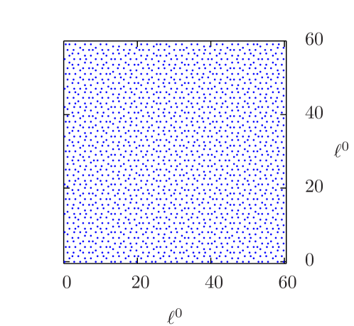
Figure 1: Positions of the vertices of the quasicrystal tiling considered in this work, in unit of $\ell^{0}$, $\ell^{0}$ being the minimum distance between 2 points of the tiling.

In this paper we focus on the specific case of a Penrose-tiled quasicrystal obtained using the Robinson triangle decomposition shown in Fig. 2. The tiling is composed with two types of tiles: the first is the triangle $\Delta_{1}^{0}$ with edges $\{\ell^{0},L^{0},L^{0}\}$, the second the triangle $\Delta_{2}^{0}$ with edges $\{L^{0},\ell^{0},\ell^{0}\}$ , with $L^{0}/\ell^{0}=\lambda$. The triangles $\Delta_{j}^{0}$ (with $j=1$ or 2) are embedded in the triangles $\Delta_{j}^{1}$ that are embedded in $\Delta_{j}^{2}$ etc…, the lengths of the edges satisfying the recursive relations $\ell^{n}=L^{n-1}$ and $L^{n}=\ell^{n-1}+L^{n-1}$ (see Fig. 2). The internal angles are equal to $\{\pi/5,2\pi/5,2\pi/5\}$ for all the triangles $\Delta_{1}^{n}$, and to $\{3\pi/5,\pi/5,\pi/5\}$ for all the triangles $\Delta_{2}^{n}$. By construction the Penrose-tiles quasicrystal is self-similar, indeed the same patterns, $\Delta_{1}^{n}$ and $\Delta_{2}^{n}$, occur at different spatial scales, but it lacks any translational symmetry (it is not a periodic crystal).

Potentials with the same symmetry as the Penrose-tiled quasicrystal can be realized in optics and microwaves with dielectric materials [3, 15] or arrays of waveguides [16], in polariton experiments by a suitable engineering of the photonic component [17, 5, 12], in ultracold atoms via the interference of five beams [4] or by using a Spatial Light Modulator (SLM) device [18].

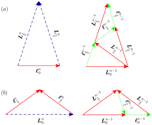
Figure 2: Robinson triangle decomposition for a Penrose tiling. (a) tiling of $\Delta_{1}^{n}$ and (b) of $\Delta_{2}^{n}$ by $\Delta_{1}^{n-1}$ and $\Delta_{2}^{n-1}$.

2 Energy-band dispersion for quasicrystals

Let us consider the subspace $\mathcal{O}_{\mathbf{k}}$ of the plane waves $W_{j,\mathbf{k}}(\mathbf{r})=e^{-i(\mathbf{k}+\tilde{\mathbf{q}}_{j})\cdot\mathbf{r}}/\sqrt{S}$, $S$ being the quasicrystal surface area. The vectors $\tilde{\mathbf{q}}_{j}$ are generated by linear combinations of the Bragg vectors $\mathbf{q}_{j}$ with relative integer coefficients, namely $\tilde{\mathbf{q}}_{j}=\sum_{i}z_{i}\mathbf{q}_{i}$. The $\mathbf{q}_{j}$ satisfy $\hat{V}(\mathbf{q}_{j})=\int e^{-i{\mathbf{q}}_{j}\cdot{\mathbf{r}}}V(\mathbf{r})d\mathbf{r}\neq 0$. Analogously to the periodic case, the subspace $\mathcal{O}_{\mathbf{k}}$ is closed under the application of the operator $H$. Thus the diagonalization of

$$\begin{split}H_{\mathbf{k}}&=\int W_{j,\mathbf{k}}(\mathbf{r})^{*}H\,W_{i,\mathbf{k}}(\mathbf{r})\,d\mathbf{r}\\ &=\dfrac{\hbar^{2}|\mathbf{k}+\tilde{\mathbf{q}}_{j}|^{2}}{2m}\delta_{i,j}+\hat{V}(\tilde{\mathbf{q}}_{i}-\tilde{\mathbf{q}}_{j}),\end{split}$$ (3)

within the subspace $\mathcal{O}_{\mathbf{k}}$, provides rigorous eigenfunctions and eigenvalues of $H$ [19]. The problem is how to associate to each eigenvalue its corresponding $\mathbf{k}$ vector. Usually a periodic approximation is done by considering the first effective BZ as adequate to describe all bands [19, 20]. But this is a rather rough approximation since, as we will show below, the BZs have different areas: for instance, the ratio between the area ${\mathcal{S}}_{2}$ of the second zone and area ${\mathcal{S}}_{1}$ of the first one is ${\mathcal{S}}_{2}/{\mathcal{S}}_{1}=\lambda-1$.

Our strategy to determine the energy-band dispersion, is the following. First we make a selection of the $\tilde{\mathbf{q}}_{j}$’s vectors, by fixing a threshold for the value of $|\hat{V}({\mathbf{q}}_{j})|^{2}$ and a maximum value of $\tilde{q}_{j}^{2}$ (this value depends on the maximum value of $k^{2}$ we are interested in). In this way we obtain a truncated finite subspace $\tilde{\mathcal{O}}_{\mathbf{k}}$ of dimension $\tilde{N}$, $\tilde{N}$ being the number of selected $\tilde{\mathbf{q}}_{j}$, and we fix the level in the hierarchy we are able to observe the gaps. Then we diagonalized $H$ whithin the subspace $\tilde{\mathcal{O}}_{\mathbf{k}}$ getting $\tilde{N}$ eigenvalues. With the aim to determine the dispersion relation $E(\mathbf{k})$, for each vector $\mathbf{k}$ we select the “physical” eigenvalue $E_{\bar{i}}$, among the $\tilde{N}$ ones, that satisfies the condition $\lim_{V_{0}\rightarrow 0}E_{\bar{i}}\rightarrow(\hbar k)^{2}/2m$. From an operational point of view, we sort the $\tilde{N}$ eigenvalues by increasing values

$$E_{1}<E_{2}<\dots E_{\tilde{N}}$$ (4)

and similarly we order the quantities $K_{j}=|{\mathbf{k}}+\tilde{\mathbf{q}}_{j}|^{2}$,

$$[K_{j}]_{1}<[K_{j}]_{2}<\dots[K_{j}]_{\tilde{N}}.$$ (5)

We select the eigenvalue $E_{\bar{i}}$ if $[K_{j}]_{\bar{i}}=k^{2}$. The points of exact degeneracy $[K_{j}]_{\alpha}=[K_{j}]_{\beta}$ are not taken into account by varing the vector ${\mathbf{k}}$ uniformly, but avoiding the points ${\mathbf{k}}=-\tilde{\mathbf{q}}_{j}$.

This procedure allows to assign each eigenvalue to the corresponding quasi-momentum and thus it defines the band structure and the extended BZ unequivocably, if they exist, without requiring the existence of a primitive cell of the reciprocal lattice, namely the system to be periodic. The variant with respect to the periodic case is that, since it does not exist a fundamental BZ, we have to repeat the procedure for any $\mathbf{k}$ vector we are interested in.

At fixed ${\mathbf{k}}$, the unselected $\tilde{N}-1$ eigenvalues correspond to eigenvalues belonging to other Brillouin zones as in the periodic case. However, away from the center of the first Brillouin zone, the lack of periodicity in the $\tilde{\mathbf{q}}_{j}$ space, makes non-trivial the allocation of these eigenvalues with respect to their corresponding Brillouin zone.

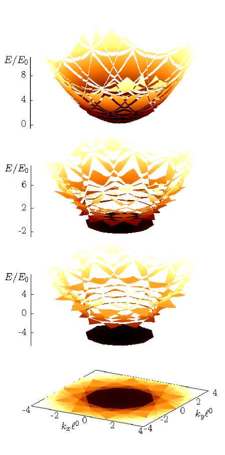
Figure 3: Energy-band dispersion $E({\mathbf{k}})$, in unit of $E_{0}=(\hbar/\ell^{0})^{2}/m$ as a function of $k_{x}$ and $k_{y}$, in unit of $1/\ell^{0}$, for a Penrose-tiled potential. From top to bottom: $V_{0}=-1$, -3, -5 $E_{0}$. The color contrast in the map view shows the extended Brillouin zones. These curves have been obtained by using $\tilde{N}=31$ and the selected vectors $\mathbf{q}_{i}$ correspond to the brightest Bragg spots (see Fig. 4), by fixing a threshold for the value of $|\hat{V}({\mathbf{q}}_{j})|^{2}$ at 0.03 $V_{0}^{2}$ and $|{\mathbf{q}}_{j}|<8/\ell^{0}$. We have verified that if we include the linear combination of these vectors in the $\tilde{\mathcal{O}}_{\mathbf{k}}$ subspace, the calculation of the spectrum does not change significantly. The inclusion of $\mathbf{q}_{i}$’s vectors corresponding to less bright Bragg spots would introduce a further fragmentation of the spectrum, which would be visible with a higher energy resolution.

The energy-band dispersion for our Penrose-tiled potential is shown in Fig. 3. For a small potential depth (top panel in Fig. 3), the dispersion law is approximately parabolic as for a free-particle, but one can already observe the opening of the gaps and the fact that the sizes of the bands, and their projections on the ${\mathbf{k}}$-plane (map view in Fig. 3), are different from each other. By increasing the potential depth (central and bottom panels in Fig. 3) the gaps open further and the bands flatten, but obviously the surface area of their projections on the ${\mathbf{k}}$-plane is independent from the potential strength. These surfaces represent the extended BZs. They look like a sunflower whose center (the first BZ) is a decagon surrounded by petals of different sizes (the higher-order BZs). Remark that the energy-band dispersion can be measured quite straightforwardly with polaritons [5, 12].

As expected from the gap labelling theory, the number of states ${\mathcal{N}}_{i}$ in each band is different from one band to another. This property is intimately connected to the splitting of the BZs, more precisely, in the limit of an infinite sample, the IDOS ${\mathcal{N}}_{i}$ of the $i$-th band is proportional to the area ${\mathcal{S}}_{i}$ of the $i$-th BZ [21]. This is due to the fact that ${\mathcal{N}}_{i}$ depend only on the geometry of the crystal and not on the strength of the potential: once the free-particle parabola is fragmented, the number of states per band is incompressible. Thus if one consider the case of a vanishing potential where the density of states is a constant $\rho(E)\sim E^{(D-2)/2}$, $D$ being the dimensionality of the system, one can easily deduce that

$${\mathcal{N}}_{i}=\int_{i-th\,{\rm band}}\!\!\!\rho(E)\,dE\propto\int_{i-th\,{\rm BZ}}\!\!\!dp^{2}={\mathcal{S}}_{i}.$$ (6)

Thus the BZs of quasicrystals can be labelled by their areas and, for a Penrose-tiled potential, there exist two integers $z_{i_{1}}$ and $z_{i_{2}}$ such that:

$${\mathcal{S}}_{i}=s_{0}(z_{i_{1}}\lambda+z_{i_{2}}).$$ (7)

3 Bragg peak labelling

The knowledge of the energy-band dispersion is not necessary to determine the BZ structure. Making a perturbative reasoning, the gaps open if two free-particle states $|{\mathbf{k}}_{i}\rangle$ and $|{\mathbf{k}}_{j}\rangle$, with the same kinetic energy, ${k}_{j}^{2}-k_{i}^{2}=0$, are coupled by the potential $V$, namely if $\hat{V}({\mathbf{k}}_{j}-{\mathbf{k}}_{i})\neq 0$, thus if $({\mathbf{k}}_{j}-{\mathbf{k}}_{i})$ is a Bragg vector ${\mathbf{q}}_{l}$ [22]. This leads to

$$({\mathbf{k}}_{j}-{\mathbf{k}}_{i})\cdot({\mathbf{k}}_{j}+{\mathbf{k}}_{i})={\mathbf{q}}_{l}\cdot(2{\mathbf{k}}_{i}+{\mathbf{q}}_{l})=0,$$ (8)

namely the boundaries of the BZs are given by the orthogonal bi-sectors of the Bragg vectors $\mathbf{q}_{l}$ as schematically illustrated in Fig. 4. Therefore the BZ labelling, and thus the gap labelling, can be indirectly deduced by a Bragg diffraction experiments. The more brillant the peak is, the more the gap will open effectively as a function of the potential strength. Thus by setting a threshold for the brightness of the peaks, we fix the level of the observable gaps, and this is exactly what we do when we select the vectors $\tilde{\mathbf{q}}_{l}$ for the calculation of the energy-band dispersion (see details of the procedure in the caption of Fig. 3).

The ensemble of the Bragg peaks at a fixed threshold for the brightness is relatively dense and the lower this threshold is, the more the number of peaks increases [23, 19]. This does not happen with periodic crystals where the number and the structure of the Bragg peaks is independent from their brightness. This intriguing phenomenon can be understood by the stability analysis of the law of recurrence used to generate the Penrose-tiled quasicrystal.

Let us consider again the Robinson triangle decomposition shown in Fig. 2. We introduce the vectorial notation

$$\boldsymbol{\ell}^{n}_{\alpha}=\ell^{n}[\cos(\alpha\pi)\,\hat{e}_{x}+\sin(\alpha\pi)\,\hat{e}_{y}],$$ (9)

where $\alpha\in\{0,1/5,2/5,\dots,9/5\}$, and analogously for $\boldsymbol{L}^{n}_{\alpha}$. For any, $n\geq 0$, it can be shown that the space $\mathcal{A}$ (${\mathbb{Z}}$-module) of all linear combination with integer coefficients of all the $\boldsymbol{\ell}^{n}_{\alpha}$’s and the $\boldsymbol{L}^{n}_{\alpha}$ is a 4-dimensional ${\mathbb{Z}}$-module and the vectors $\boldsymbol{\ell}^{n}_{0},\boldsymbol{\ell}^{n}_{1/5},\boldsymbol{\ell}^{n}_{2/5},\boldsymbol{\ell}^{n}_{3/5},$ form a basis of this module. In this basis, it is easy to check that matrix giving recurrence law for the generation of the Penrose tiling (i.e. the matrix that gives the expression of $\boldsymbol{\ell}^{n+1}_{0},\boldsymbol{\ell}^{n+1}_{1/5},\boldsymbol{\ell}^{n+1}_{2/5},\boldsymbol{\ell}^{n+1}_{3/5},$ as linear combination with integer coefficient of the vectors $\boldsymbol{\ell}^{n}_{0},\boldsymbol{\ell}^{n}_{1/5},\boldsymbol{\ell}^{n}_{2/5},\boldsymbol{\ell}^{n}_{3/5}$) is given by

$$\mathcal{M}=\left(\begin{matrix}1&0&1&-1\\ 1&0&1&0\\ 0&1&0&1\\ -1&1&0&1\\ \end{matrix}\right).$$ (10)

The eigenvectors of $\mathcal{M}$ are ${\mathbf{v}}_{+1,+2}^{n}$ with components $(-\lambda,-1,0,1)$ and $(\lambda,\lambda,1,0)$ and eigenvalues ${m}_{+1}=m_{+2}=\lambda$, and ${\mathbf{v}}_{-1,-2}^{n}$ with components $(\lambda-1,-1,0,1)$ and $(1-\lambda,1-\lambda,1,0)$ and eigenvalues ${m}_{-1}=m_{-2}=1-\lambda$. Thus, under iteration, vectors that belong to the stable eigenspace generated by ${\mathbf{v}}_{-1}^{n}$ and ${\mathbf{v}}_{-2}^{n}$ converge to zero exponentially fast.

The diffraction pattern $I(\mathbf{r})$ of $V(\mathbf{r})$ shown in Fig. 4 is given by

$$I(\mathbf{r})\propto\left|\hat{V}(\mathbf{k})\right|^{2}=\left|\int e^{-i{\mathbf{k}}\cdot{\mathbf{r}}}V(\mathbf{r})d\mathbf{r}\right|^{2}=V_{0}^{2}\left|\sum_{j}e^{-i{\mathbf{k}}\cdot{\mathbf{r}}_{j}}\right|^{2}.$$ (11)

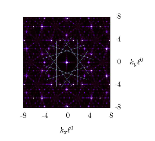
Figure 4: Bragg diffraction of a Penrose-tiled potential formed by 1700 potential wells distributed on a square of side $60\ell^{0}$ (see Fig. 1). The lines are the orthogonal bi-sectors of the brightest ${\mathbf{k}}$ Bragg vectors and show the boundaries of the first BZs.

It is known that for the Penrose-tiled quasicrystal (or more generally for a larger class of substitution tilings) the Bragg peaks correspond to the values of ${\mathbf{k}}$ such that for any $\alpha\in\{0,1/5,2/5,\dots,9/5\}$, the quantities $e^{-i{\mathbf{k}}\cdot{\boldsymbol{L}^{n}_{\alpha}}}$ and $e^{-i{\mathbf{k}}\cdot{\boldsymbol{\ell}^{n}_{\alpha}}}$ converge to 1 exponentially fast as $n$ goes to $+\infty$ (see [24, 25, 26, 27]). Since the vectors $\boldsymbol{\ell}^{n}_{0},\boldsymbol{\ell}^{n}_{1/5},\boldsymbol{\ell}^{n}_{2/5},\boldsymbol{\ell}^{n}_{3/5},$ form a basis of $\mathcal{A}$, it is enough to show the convergence of $e^{-i{\mathbf{k}}\cdot{\boldsymbol{\ell}^{n}_{\alpha}}}$ for $\alpha=0,1/5,2/5,3/5$. Notice that, for $\alpha=(j-1)/5$,

$$\begin{split}{\mathbf{k}}\cdot{\boldsymbol{\ell}^{n}_{\alpha}}={\mathbf{k}}\cdot{\sum_{j=1}^{j=4}m^{n}_{i,j}{\boldsymbol{\ell}^{0}_{(j-1)/5}}={\sum_{j=1}^{j=4}m^{n}_{i,j}{\mathbf{k}}\cdot{\boldsymbol{\ell}^{0}_{(j-1)/5}}}}\end{split}$$ (12)

where $m^{n}_{i,j}$ is the coefficient at the $i^{th}$ line and $j^{th}$ column of the matrix $\mathcal{M}$.

It follows from the above discussion that the condition for ${\mathbf{k}}$ to be a Bragg peak is that the vector ${\boldsymbol{\xi}}^{n}=(\mathbf{k}\cdot\boldsymbol{\ell}^{n}_{0},\mathbf{k}\cdot\boldsymbol{\ell}^{n}_{\frac{1}{5}},\mathbf{k}\cdot\boldsymbol{\ell}^{n}_{\frac{2}{5}},\mathbf{k}\cdot\boldsymbol{\ell}^{n}_{\frac{3}{5}})$ belongs to the stable eigenspace of the matrix $\mathcal{M}$ modulo a translation on the lattice $2\pi{\mathbb{Z}}^{4}$. That is

$${\boldsymbol{\xi}}^{0}+(2p_{1}\pi,2p_{2}\pi,2p_{3}\pi,2p_{4}\pi)=\alpha{\mathbf{v}}_{-1}^{0}+\beta{\mathbf{v}}_{-2}^{0},$$ (13)

for $p_{i}$’s in ${\mathbb{Z}}$. This condition is fulfilled if

$$\begin{split}&k_{x}\ell^{0}=\dfrac{2\pi}{3-\lambda}[p_{1}-p_{3}+p_{4}+\lambda(p_{3}-p_{4})]\\ &k_{y}\ell^{0}=\dfrac{2\pi[-p_{1}+2p_{2}+p_{4}-p_{3}+\lambda(p_{4}+p_{3})]}{2[\sin(3\pi/5)+2\sin(\pi/5)]}.\\ \end{split}$$ (14)

The brighest peaks visible in Fig. 4 correspond to the smallest values of $||\alpha{\mathbf{v}}_{-1}^{0}+\beta{\mathbf{v}}_{-2}^{0}||$; for these values, the convergence to 1 of the terms $e^{-i{\mathbf{k}}\cdot{\boldsymbol{L}^{n}_{\alpha}}}$ and $e^{-i{\mathbf{k}}\cdot{\boldsymbol{\ell}^{n}_{\alpha}}}$ is achieved more rapidly. In Fig. 5 we show some Bragg peak positions as predicted by Eqs. (LABEL:bellissime). We selected them by choosing a maximum threshold for the value of $||\alpha{\mathbf{v}}_{-1}^{0}+\beta{\mathbf{v}}_{-2}^{0}||$: 20 for the gray crosses and 5 for the red squares. These latter correspond to the brightest peaks in Fig. 4.

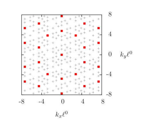
Figure 5: Bragg peaks for a Penrose-tiled quasicrystal calculated by using Eqs. (LABEL:bellissime). The gray cosses correspond to $||\alpha{\mathbf{v}}_{-1}^{0}+\beta{\mathbf{v}}_{-2}^{0}||<20$, while the red squares correspond to $||\alpha{\mathbf{v}}_{-1}^{0}+\beta{\mathbf{v}}_{-2}^{0}||<5$.

4 Conclusions

We develop a very straightforward method to calculate the energy-band dispersion for quasicrystals as a function of the extended Brillouin zones. Our strategy allows to do without the rough approximation exploited usually in the literature to assume that the first Brillouin zone can be considered as the fundamental one. The connection between the spectrum and the quasi-momentum space raises the natural connection between the integrated density-of-states per band and the area of the corresponding Brillouin zone, transposing the gap labelling to a Brillouin zone labelling. Moreover we label the Brillouin zones by labelling the Bragg vectors. By using the recursive law of generation of a Penrose-tiled quasicrystal we find an analytical expression that gives the Bragg vectors and we are able to identify the ones that correspond to the brightest Bragg peaks.

Our study offers the realistic possibility to measure the gap labelling within an optics experiment [3], polaritons [5] or with ultracold atoms [13]. In this context, the extended Brillouin zones can be measured one by one (i) transfering a Bose-Einstein condensate in the corresponding band by a Raman transition, (ii) populating homogenously the band via Bloch oscillations, (iii) ramping down the potential to project the band over the free-particle paraboloid and (iv) doing a time-of-flight imaging to have access to the (quasi-) momentum distribution [13, 14, 28]. The measure of the areas of the different momentum distributions, that correspond to different Brillouin zones, would provide an experimental proof of the gap labelling theory.

References

- Shechtman et al. [1984] D. Shechtman, I. Blech, D. Gratias, and J. W. Cahn. Metallic phase with long-range orientational order and no translational symmetry. Phys. Rev. Lett., 53:1951–1953, Nov 1984. doi: 10.1103/PhysRevLett.53.1951. URL http://link.aps.org/doi/10.1103/PhysRevLett.53.1951.
- Bindi et al. [2009] L. Bindi, P. J. Steinhardt, N. Yao, and P. J. Lu. Natural quasicrystals. Science, 324:1306, 2009.
- Man et al. [2005] Weining Man, Mischa Megens Megens, Paul J. Steinhardt, and P.M. Chaikin. Experimental measurement of the photonic properties of icosahedral quasicrystals. Nature, 436:993, May 2005. doi: 10.1038/nature03977. URL http://dx.doi.org/10.1038/nature03977.
- Guidoni et al. [1999] L. Guidoni, B. Dépret, A. di Stefano, and P. Verkerk. Atomic diffusion in an optical quasicrystal with five-fold symmetry. Phys. Rev. A, 60:R4233–R4236, Dec 1999. doi: 10.1103/PhysRevA.60.R4233. URL http://link.aps.org/doi/10.1103/PhysRevA.60.R4233.
- Tanese et al. [2013a] D. Tanese, E. Gurevich, A. Lemaître, E. Galopin, I. Sagnes, A. Amo, J. Bloch, and E. Akkermans. Fractal energy spectrum of a polariton gas in a Fibonacci quasi-periodic potential. Phys. Rev. Lett, 112:14604, Apr 2014. doi: 10.1103/PhysRevLett.112.146404. URL http://journals.aps.org/prl/abstract/10.1103/PhysRevLett.112.146404.
- Bellissard [1993] J. Bellissard. Gap labelling theorems for Schrödinger’s operators. In J.M. Luck, P. Moussa, and M. Waldschmidt, editors, From Number Theory to Physics, Les Houches March 89, pages 538–630. Springer, 1993.
- Benameur and Oyono-Oyono [2003] M.-T. Benameur and H. Oyono-Oyono. Gap-labelling for quasi-crystals (proving a conjecture by j. bellissard). In J. M. Combes and et al., editors, Operator Algebras and Mathematical Physics (Constanta 2001), pages 11–22. Theta, 2003.
- Kaminker and Putnam [2003] J. Kaminker and I. Putnam. A proof of the gap labeling conjecture. Michigan Math. J., 51:537–546, 2003.
- Bellissard et al. [2006] J. Bellissard, R. Benedetti, and J. M. Gambaudo. Finite telescopic approximations and gap-labelling. Commun. Math. Phys., 261:1–41, 2006.
- Lang et al. [2012] Li-Jun Lang, Xiaoming Cai, and Shu Chen. Edge states and topological phases in one-dimensional optical superlattices. Phys. Rev. Lett., 108:220401, May 2012. doi: 10.1103/PhysRevLett.108.220401. URL http://link.aps.org/doi/10.1103/PhysRevLett.108.220401.
- Cai et al. [2011] Xiaoming Cai, Shu Chen, and Yupeng Wang. Quantum criticality in disordered bosonic optical lattices. Phys. Rev. A, 83:043613, Apr 2011. doi: 10.1103/PhysRevA.83.043613. URL http://link.aps.org/doi/10.1103/PhysRevA.83.043613.
- Jacqmin et al. [2013] T. Jacqmin, I. Carusotto, I. Sagnes, M. Abbarchi, D. Solnyshkov, G. Malpuech, E. Galopin, A. Lemaître, J. Bloch, and A. Amo. Direct observation of Dirac cones and a flatband in a honeycomb lattice for polaritons. Phys. Rev. Lett, 112:116402, Mar 2014. doi: 10.1103/PhysRevLett.112.116402. URL http://journals.aps.org/prl/abstract/10.1103/PhysRevLett.112.116402.
- Greiner et al. [2001] Markus Greiner, Immanuel Bloch, Olaf Mandel, Theodor W. Hänsch, and Tilman Esslinger. Exploring phase coherence in a 2d lattice of Bose-Einstein condensates. Phys. Rev. Lett., 87:160405, Oct 2001. doi: 10.1103/PhysRevLett.87.160405. URL http://link.aps.org/doi/10.1103/PhysRevLett.87.160405.
- Wirth et al. [2011] Georg Wirth, Matthias Ölschläger , and Andreas Hemmerich. Evidence for orbital superfluidity in the P-band of a bipartite optical square lattice Nat. Phys., 7:147, 2011. doi: 10.1038/nphys1857. URL http://www.nature.com/nphys/journal/v7/n2/full/nphys1857.html.
- Bellec et al. [2013] Matthieu Bellec, Ulrich Kuhl, Gilles Montambaux, and Fabrice Mortessagne. Topological transition of Dirac points in a microwave experiment. Phys. Rev. Lett., 110:033902, Jan 2013. doi: 10.1103/PhysRevLett.110.033902. URL http://link.aps.org/doi/10.1103/PhysRevLett.110.033902.
- Rechtsman et al. [2013] Mikael C. Rechtsman, Yonatan Plotnik, Julia M. Zeuner, Daohong Song, Zhigang Chen, Alexander Szameit, and Mordechai Segev. Topological creation and destruction of edge states in photonic graphene. Phys. Rev. Lett., 111:103901, Sep 2013. doi: 10.1103/PhysRevLett.111.103901. URL http://link.aps.org/doi/10.1103/PhysRevLett.111.103901.
- Tanese et al. [2013b] D. Tanese, H. Flayac, D. Solnyshkov, A. Amo, A. Lemaitre, E. Galopin, R. Braive, P. Senellart, I. Sagnes, G. Malpuech, and J. Bloch. Polariton condensation in solitonic gap states in a one-dimensional periodic potential. Nat. Commun., 4:1749, 2013b.
- Barboza et al. [2013] R. Barboza, U. Bortolozzo, G. Assanto, E. Vidal-Henriquez, M. G. Clerc, and S. Residori. Harnessing optical vortex lattices in nematic liquid crystals. Phys. Rev. Lett., 111:093902, Aug 2013. doi: 10.1103/PhysRevLett.111.093902. URL http://link.aps.org/doi/10.1103/PhysRevLett.111.093902.
- Kaliteevski et al. [2000] MA Kaliteevski, S Brand, RA Abram, TF Krauss, R DeLa Rue, and P Millar. Two-dimensional penrose-tiled photonic quasicrystals: from diffraction pattern to band structure. Nanotechnology, 11(4):274–280, 2000. ISSN 0957-4484.
- Florescu et al. [2009] Marian Florescu, Salvatore Torquato, and Paul J. Steinhardt. Complete band gaps in two-dimensional photonic quasicrystals. Phys. Rev. B, 80:155112, Oct 2009. doi: 10.1103/PhysRevB.80.155112. URL http://link.aps.org/doi/10.1103/PhysRevB.80.155112.
- Luck [1989] J. M. Luck. Cantor spectra and scaling of gap widths in deterministic aperiodic systems. Phys. Rev. B, 39:5834–5849, Mar 1989. doi: 10.1103/PhysRevB.39.5834. URL http://link.aps.org/doi/10.1103/PhysRevB.39.5834.
- Grosso and Pastori Parravicini [2000] Giuseppe Grosso and Giuseppe Pastori Parravicini. Solid State Physics. Academic Press, 2000.
- Elser [1985] Veit Elser. Indexing problems in quasicrystal diffraction. Phys. Rev. B, 32:4892–4898, Oct 1985. doi: 10.1103/PhysRevB.32.4892. URL http://link.aps.org/doi/10.1103/PhysRevB.32.4892.
- Dworkin [1993] S. Dworkin. Spectral theory and x -ray diffraction. J. Math. Phys., 34:2965–2967, 1993.
- Lee et al. [2002] J.-Y. Lee, R.V. Moody, and B. Solomyak. Pure point dynamical and diffraction spectra. Ann. Henri Poincaré, 3:1003–1018, 2002.
- Solomyak [2007] B. Solomyak. Eigenfunctions for substitution tiling systems. Advanced Studies in Pure Mathematics, 49:433–454, 2007.
- Barge and Kwapisz [2006] M. Barge and J. Kwapisz. Geometric theory of unimodular pisot substitutions. Amer. J. Math., 128:1219–1282, 2006.
- Greiner [2003] Markus Greiner. Ultracold quantum gases in three-dimensional optical lattice potentials. PhD thesis, Universität München, 2003.